Perturbative QCD concerning light and heavy flavor in the EPOS4 framework

We recently introduced new concepts, implemented in EPOS4, which allows us to consistently accommodate factorization and saturation in high-energy proton-proton and nucleus-nucleus collisions, in a rigorous parallel scattering framework. EPOS4 has a modular structure and in this paper, we present in detail how the “single scattering module” (the main EPOS4 building block) is related to perturbative QCD, and how these calculations are performed, with particular care being devoted to heavy flavor contributions. We discuss similarities and differences compared to the usual pQCD approach based on factorization.
   

1 Introduction

Factorization [1, 2] (in connection with asymptotic freedom [3, 4]) is a powerful concept to reliably compute inclusive cross sections for high transverse momentum ($p_{t}$) particle production in proton-proton (pp) scattering at very high energies. However, there are very interesting cases not falling into this category, like high-multiplicity events in proton-proton scattering in the TeV energy range, where a very large number of parton-parton scatterings contribute. Such events are particularly interesting, since the CMS collaboration observed long-range near-side angular correlations for the first time in high-multiplicity proton-proton collisions [5], which was before considered to be a strong signal for collectivity in heavy-ion collisions. Studying such high-multiplicity events (and multiplicity dependencies of observables) goes much beyond the frame covered by factorization, and we need an appropriate tool, able to deal with multiple scatterings, which must happen in parallel at high energies.

Although everybody will agree that multiple scatterings should conserve energy-momentum, the way it is implemented is fundamentally different in EPOS compared to other models. Concerning momentum sharing, the EPOS4 method employs multiple scattering laws of the form $f_{1}(p_{1})\times f_{2}(p_{2})..\times\delta(p-\sum p_{i})$. The delta function here is crucial, like the probability law in a microcanonical ensemble. We refer to this method as “rigorous parallel scattering scenario”, for unbiased momentum sharing. This is very different compared to a structure like $f_{1}(p_{1}|p)\times f_{2}(p_{2}|p-p_{1})\times f_{3}(p_{3}|p-p_{1}-p_{2})$ with conditional probabilities (as it is usually done), which may perfectly conserve momentum but in a sequential manner.

In [6], we show that such a “rigorous parallel scattering scheme” can be constructed based on S-matrix theory (see also [7, 8, 9, 10, 11]), which we will briefly review in the following. We show – and this is far from trivial – how to accommodate factorization and saturation in an energy conserving parallel scattering scenario. The starting point is the elastic scattering T-matrix

$$iT=\sum_{n=0}^{\infty}\int dX\,\frac{1}{n!}\,V\times\left\{iT_{\mathrm{Pom}}\times...\times iT_{\mathrm{Pom}}\right\}\times V\times\delta,$$ (1)

expressed in terms of “elementary” T-matrices $T_{\mathrm{Pom}}$, the latter ones representing parton-parton scattering, with the “vertex” V representing the connection to the projectile and target remnants. The elementary T-matrices depend on the light-cone momentum fractions $x_{i}^{\pm}$of the incoming partons, in addition to the energy squared $s$, and the impact parameter $b$. The vertices depend on the light-cone momentum fractions of the remnants $x_{\mathrm{remn}}^{+}$ (projectile side) or $x_{\mathrm{remn}}^{-}$ (target side). Most important: the $\delta$ which stands for

$$\delta(1-\sum x_{i}^{+}-x_{\mathrm{remn}}^{+})\delta(1-\sum x_{i}^{-}-x_{\mathrm{remn}}^{-}),$$ (2)

to assure energy-momentum conservation in an unbiased fashion (this is what we mean by a rigorous parallel scattering scenario). The symbol $\int dX$ stands for integrating over all these momentum fractions. The expression can be easily generalized for nucleus-nucleus scattering [6].

So far we discussed only elastic scattering, the connection with inelastic scattering provides the optical theorem in impact parameter representation,

$$\sigma_{\mathrm{tot}}=\int d^{2}b\,\mathrm{cut}\,T,$$ (3)

with $\mathrm{cut\,}T\equiv\mathrm{\frac{1}{i}disc}T$, where $\mathrm{disc}\,T$ is the s-channel discontinuity $T(s+i\epsilon)-T(s-i\epsilon),$ and with $T$ being per definition the Fourier transformed T-matrix divided by $2s$. So we need to compute the “cut” of the complete diagram, $\mathrm{cut}\,T$, i.e., for pp we need to evaluate

$$\mathrm{cut}\left\{V\times iT_{\mathrm{Pom}}\times...\times iT_{\mathrm{Pom}}\times V\right\},$$ (4)

which corresponds to the sum of all possible cuts, considering, in particular, all possibilities of cutting or not any of the parallel Pomerons. We have finally a sum of products with some fraction of the Pomerons being cut (cut Pomerons), the others not (uncut Pomerons), referred to as cutting rules. We define $G$ to be the cut of a single Pomeron,

$$G=\mathrm{cut}\,T_{\mathrm{Pom}}.$$ (5)

Cut Pomerons represent inelastic scattering ( $a+b\to$ many partons) and uncut Pomerons elastic scatterings ($a+b\to a+b$).

The uncut Pomerons are finally summed over and the corresponding variables integrated out, so eventually the total cross section is expressed as a sum over products of $G$, very similar to Eq. (1) with the vertices $V(x_{\mathrm{remn}}^{+})V(x_{\mathrm{remn}}^{-})$ replaced by some effective vertex function $W(x_{\mathrm{remn}}^{+},x_{\mathrm{remn}}^{-})$. A great advantage of this T-matrix formalism is its modular structure. Multiple scattering is expressed in terms of modules ($G$) representing a single scattering each, as shown in the case of two inelastic scatterings in Fig. 1.

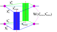
Figure 1: Double scattering, each box representing a cut Pomeron (single inelastic scattering).

The precise content of these modules will be discussed later - this is where all the perturbative QCD physics is hidden, and discussing that will be the main purpose of this paper.

The important new issue in [6] is the understanding of how energy conservation ruins factorization, and how to solve this problem via an appropriate definition of $G$. The cut Pomeron $G=\mathrm{cut\,}T_{\mathrm{Pom}}$ is the fundamental quantity in the EPOS formalism. For the moment, we consider the Pomeron as a “box”, with two external legs representing two incoming particles (nucleon constituents) carrying light-cone momentum fractions $x^{+}$ and $x^{-}$, so $G=G(x^{+},x^{-},s,b)$, with the energy squared $s$, and the impact parameter $b$, see Fig. 2.

$$\boldsymbol{\boldsymbol{=G(x^{+},x^{-},s,b)}}$$

Figure 2: The cut Pomeron $G$.

Let us define the “Pomeron energy fraction” $x_{\mathrm{PE}}=x^{+}x^{-}=M_{\mathrm{Pom}}^{2}/s,$ with $M_{\mathrm{Pom}}$ being the transverse mass of the Pomeron, which is the crucial variable characterizing cut Pomerons: the bigger $x_{\mathrm{PE}}$, the bigger the Pomeron’s invariant mass and the number of produced particles. Large invariant masses also favor high $p_{t}$ jet production. We also define, for a given cut Pomeron connected to projectile nucleon $i$ and target nucleon $j$, a “connection number” $N_{\mathrm{conn}}=(N_{\mathrm{P}}+N_{\mathrm{T}})/2,$ with $N_{\mathrm{P}}$ being the number of Pomerons connected to i, and with $N_{\mathrm{T}}$ being the number of Pomerons connected to j. The case $N_{\mathrm{conn}}=1$ corresponds to an isolated Pomeron, which may take all the energy of the initial nucleons, whereas in the case of $N_{\mathrm{conn}}>1$ the energy for a given Pomeron will be shared with others. To quantify the effect of energy sharing, we define $f^{(N_{\mathrm{conn}})}(x_{\mathrm{PE}}$) to be the inclusive $x_{\mathrm{PE}}$ distribution , i.e., the probability that a single Pomeron carries an energy fraction $x_{\mathrm{PE}}$, for Pomerons with given values of $N_{\mathrm{conn}}$. The distribution for $N_{\mathrm{conn}}>1$ will be deformed with respect to the $N_{\mathrm{conn}}=1$ case, due to energy sharing, and we define the corresponding “deformation function” $R_{\mathrm{deform}}(x_{\mathrm{PE}})$ as a ratio of $f^{(N_{\mathrm{conn}})}(x_{\mathrm{PE}}$) over $f^{(1)}(x_{\mathrm{PE}}$). As shown in [6], this function can be calculated and tabulated. As discussed in very much detail later, we also calculate and tabulate some function $G_{\mathrm{QCD}}(Q^{2},\,x^{+},x^{-},s,b)$, which contains as a basic element a cut parton ladder based on DGLAP parton evolutions [9, 12, 13] from the projectile and target side, with an elementary QCD cross section in the middle, $Q^{2}$ being the low virtuality cutoff in the DGLAP evolution. The latter is usually taken to be constant and of the order of $1\,$GeV, whereas we allow any value. With all this preparation, we are now able to connect $G$ (used in the multi-Pomeron diagrams) and $G_{\mathrm{QCD}}$ (making the link to QCD), as follows:

For each cut Pomeron, for given $x^{\pm}$, $s$, $b$, and $N_{\mathrm{conn}}$, we postulate: $$\boldsymbol{G(\!\,x^{+}\!\!,x^{-}\!\!,s,b)\!=\frac{n}{R_{\mathrm{deform}}^{(N_{\mathrm{conn}})}(x_{\mathrm{PE}})}G_{\mathrm{QCD}}(Q_{\mathrm{sat}}^{2}\,,\,x^{+}\!\!,x^{-}\!\!,s,b)},$$ (6)
with $n$ being independent on $x^{\pm}$. Most importantly, $G$ does not depend on $N_{\mathrm{conn}}$, but $Q_{\mathrm{sat}}^{2}$ does, it “compensates” the $N_{\mathrm{conn}}$ dependence of $R_{\mathrm{deform}}^{(N_{\mathrm{conn}})}$. Considering even a large value of $N_{\mathrm{conn}}$, we can prove that the distribution $f^{(N_{\mathrm{conn}})}(x_{\mathrm{PE}}$) is proportional to a product of vertex functions times $G_{\mathrm{QCD}}(Q_{\mathrm{sat}}^{2}\,,\,x^{+}\!\!,x^{-}\!\!,s,b)$, and so the deformation cancels out! So, for any number of $N_{\mathrm{conn}}$, the inclusive particle production is governed by a single Pomeron represented by $G_{\mathrm{QCD}}$, which does not depend on $N_{\mathrm{conn}}$, apart from the implicit $N_{\mathrm{conn}}$ dependence of $Q_{\mathrm{sat}}^{2}$. Consequently, the $p_{t}$ dependence of outgoing partons will be independent of $N_{\mathrm{conn}}$ in the hard domain (high $p_{t}$), see [6] for more details. Computing a $p_{t}$ distribution according to $G_{\mathrm{QCD}}$ amounts precisely to factorization or binary scaling in AA scattering, but - again - only obtained for hard processes. In other words, computing $R_{\mathrm{AA}}$ in a full AA simulation, we get unity at large $p_{t}.$

Let us come back to our earlier statement saying that “energy conservation ruins factorization”. The statement actually depends on how one relates $G$ and $G_{\mathrm{QCD}}$. In earlier versions, we adopted what we thought at the time to be “the natural Pomeron definition”, but what we now call “the naive Pomeron definition”, namely $G=G_{\mathrm{QCD}}$. As discussed in very much detail in [6], this leads unavoidably to the following problem: An inclusive pp $p_{t}$ distribution will be a superposition of contributions for different connection numbers. With increasing connection numbers, these contributions get more and more deformed (suppressed at large $x_{{\rm PE}}$), which corresponds to a suppression of the yields at high $p_{t}$. Therefore the minimum bias $p_{t}$ distribution will be suppressed at large $p_{t}$ compared to the single Pomeron distribution. On the other hand, factorization requires inclusive cross sections to be given by a single cut Pomeron, since based on this diagram one obtains formulas as $f_{{\rm PDF}}\otimes\hat{\sigma}\otimes f_{{\rm PDF}}$, corresponding to factorization.

The fact that multiple Pomeron interactions reduce for inclusive cross sections to a single cut Pomeron (leading to factorization if one assumes “the naive Pomeron definition”), refers to “AGK cancellations” [10], shown to be valid in a scenario without energy conservation. As discussed above, including energy sharing (as it should be), ruins first “AGK cancellations” and, as a consequence, factorization. With a “proper Pomeron definition” as employed in EPOS4, we recover “AGK cancellations” in the sense that inclusive cross sections can be expressed in terms of a single Pomeron expression $G_{\mathrm{QCD}}$, although in reality multiple scatterings contribute. But this statement is only true for $p_{t}$ values bigger than the relevant saturation scales of the different multiple scattering contributions, where “relevant” refers to the relative weight of the contributions.

The new EPOS4 framework is able to recover factorization at large $p_{t}$ (a difficult task in the parallel scattering formalism). This allows us to compute, tabulate, and employ “EPOS PDFs”, and based on these, we may compute inclusive cross sections as a simple convolution of two PDFs and an elementary pQCD cross section, and the result will be identical – at large $p_{t}$ – to the simulation results. But to make this work in practice, we need high precision and appropriate methods for both simulation and cross section calculations. In older versions, for example, we used in the simulations frequently a “redo” whenever “kinematic problems” showed up, whereas such situations should be avoided.

As a side remark, the EPOS4 multiple scattering scheme is quite different to what is usually called ’multiple parton interactions’ (MPI): the former refers to multiple cut Pomerons with external legs being soft partons, whereas the latter treats the scattering of two hard partons, based on multiple parton distribution functions, generalizing the factorization approach. The review [14] has actually two parts, namely “hard MPI” and “soft MPI”, and the two have little in common.

The main purpose of this paper is to provide detailed information about the calculation of $G_{\mathrm{QCD}}$, based on perturbative QCD, with special care concerning heavy flavors. We discuss the implementation (for the first time in the EPOS framework) of the “backward parton evolution method”, which allows much better control of the hard processes. We discuss important “kinematic” issues connected to processes involving charm and bottom, taking into account 12 different “reaction classes” for the cross section calculations, since the kinematics is quite different, e.g., for the Born processes $gg\to gg$ and $gg\to b\bar{b}$. A useful side-effect concerning the new strategies, in particular the “backward evolution”, is the fact that many formulas are very similar to what is used in models based on “factorization”. We may compare our EPOS PDFs with “standard” PDFs, but there are also fundamental differences: in EPOS, we have first to deal with evolutions for each parton ladder, with an initial distribution of the corresponding parton distribution of the type $\delta(1-x)$, and these singularities need to be taken care of. Related to this, dealing with singularities is the major challenge for cross section calculations as well as for parton generation.

We mentioned already the modular structure of the approach, where the multiple scattering is expressed in terms of the cut Pomerons $G$, and the latter one corresponds to some function $G_{\mathrm{QCD}}$. This function $G_{\mathrm{QCD}}$ itself has a modular structure, the modules being vertex functions, a soft evolution function, and most importantly the “cut parton ladder”, which is (up to an impact parameter dependent factor) equal to a parton-parton cross section. In section 2, we will discuss how the EPOS4 building block $G_{\mathrm{QCD}}$ is related to parton-parton cross sections, and in section 3, we will discuss how the integrated and differential parton-parton cross sections can be computed. The former are needed to compute $G_{\mathrm{QCD}}$, while the latter are necessary for the parton generation.

2 Relating the EPOS4 building block $\boldsymbol{\boldsymbol{G_{\mathrm{QCD}}}}$ to parton-parton cross sections

As discussed in the last section (see also [6]), the multiple scattering contributions to the total cross section are expressed in terms of (products of) cut Pomeron expressions $G$, and the latter ones are related the “real QCD expressions” $G_{\mathrm{QCD}}$ via Eq. (6). In this sense, $G_{\mathrm{QCD}}$ is the basis of everything, the fundamental building block of EPOS4. This $G_{\mathrm{QCD}}$ depends on the saturation scale $Q_{\mathrm{sat}}^{2}$, which is of fundamental importance in the EPOS4 framework [6], but here the focus is on the details for the calculation of $G_{\mathrm{QCD}}$, where $Q_{\mathrm{sat}}^{2}$ is “only” a constant, representing the low virtuality cutoff (and we use simply symbols like $Q_{1}^{2}$ and $Q_{2}^{2}$ as arguments).

We will use different symbols, like $G$, $T$, $\boldsymbol{\mathrm{T}}$, and $\sigma$, all being related to each other. For clarity, we recall the definitions in Table 1.

$\boldsymbol{\mathrm{T}}$	Diagonal element of the elastic scattering T-matrix as defined in standard quantum mechanics textbooks, where the asymptotic state is a system of two protons or two nuclei
$T$	Fourier transform with respect to the transverse momentum exchange of the elastic scattering T-matrix $\boldsymbol{\mathrm{T}}$, divided by $2s$ (formulas are simpler using this representation)
$G$	Defined as $G=\mathrm{cut}\,T=2\mathrm{Im}T=\frac{1}{i}\mathrm{disc}T$ (where “disc” refers to the variable $s$), referring to the inelastic process associated with the cut of the elastic diagram corresponding to $T$
$\sigma$	Integrated inclusive parton-parton scattering cross section, which is useful because $\boldsymbol{\mathrm{T}}$, $T$, and $G$ may be expressed in terms of $\sigma$

Table 1: The symbols $G$, $T$, $\boldsymbol{\mathrm{T}}$, and $\sigma$.

Concerning the structure of $G_{\mathrm{QCD}}$, we expect on both projectile and target side two possibilities, namely a valence quark or a sea quark/gluon being the first perturbative parton, and in addition soft contributions, correspondingly we have

$$G_{\mathrm{QCD}} =G_{\mathrm{QCD}}^{\mathrm{sea-sea}}+G_{\mathrm{QCD}}^{\mathrm{sea-val}}+G_{\mathrm{QCD}}^{\mathrm{val-sea}}+G_{\mathrm{QCD}}^{\mathrm{val-val}}$$

$$+G_{\mathrm{soft}}+G_{\mathrm{psoft}}.$$ (7)

In this section, we will discuss the different $G$’s one by one, and in particular how the $G_{\mathrm{QCD}}^{K}$ are related to parton-parton cross sections $\sigma$, the latter one discussed in great detail in section 3.

2.1 The usual factorization approach for proton-proton scattering

Certain elements of the EPOS4 scheme are similar to the usual factorization approach, which we will briefly review in the following. Based on the factorization hypothesis, the inclusive parton production cross section in proton-proton scattering is given as [2]

$$E_{3}E_{4}\frac{d^{6}\sigma_{\mathrm{incl}}}{d^{3}p_{3}d^{3}p_{4}}=\sum_{klmn}\int\!\int\!\!dx_{1}dx_{2}\,f_{\mathrm{PDF}}^{k}(x_{1},\mu_{\mathrm{F}}^{2})f_{\mathrm{PDF}}^{l}(x_{2},\mu_{\mathrm{F}}^{2})$$

$$\qquad\frac{1}{32s\pi^{2}}\bar{\sum}|\mathcal{M}^{kl\to mn}|^{2}\delta^{4}(p_{1}+p_{2}-p_{3}-p_{4})\frac{1}{1+\delta_{mn}},$$ (8)

where the parton distribution function (PDF) $f_{\mathrm{PDF}}^{a}$ represents the number of partons of species $a$ entering the hard scattering, and where $p_{1}$ and $p_{2}$ ($p_{3}$ and $p_{4}$) are the momenta of the incoming (outgoing) partons. The PDFs can be considered to be known from deep inelastic electron-proton scattering, the amplitudes $\mathcal{M}$ can be computed, and thus one obtains the inclusive cross section as a simple integral. The factorization scale $\mu_{\mathrm{F}}^{2}$ represents the scale which allows to separate “long range (soft)” and “short range (hard)” parts of the interaction, such that the former ones are part of the proton structure, whereas the latter ones show up in the perturbative matrix elements $\mathcal{M}$. This procedure has been shown to successfully describe experimental jet production data. In the EPOS4 framework, a similar “factorization formula” will be used but in a different context.

2.2 Cut parton ladder $\boldsymbol{\boldsymbol{G_{\mathrm{QCD}}^{\mathrm{hard}}}}$ and the parton-parton cross section $\boldsymbol{\boldsymbol{\sigma_{\mathrm{hard}}^{ij}}}$

We first discuss a somewhat simplified situation, namely a simple parton ladder. Let us consider the scattering of two partons with flavors $i$ and $j$ carrying virtualities $Q_{1}^{2}$ and $Q_{2}^{2}$ , both first evolving via parton emissions with ordered virtualities up to $\mu_{F}^{2}$ before interacting as an elementary $2\to 2$ pQCD (hard) scattering (see Fig. 3).

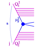
Figure 3: The parton-parton cross section $\sigma_{\mathrm{hard}}^{ij}(Q_{1}^{2},Q_{2}^{2},s)$.

The corresponding di-jet production cross section can be written as

$$\sigma_{\mathrm{hard}}^{ij}(Q_{1}^{2},Q_{2}^{2},s)=\sum_{klmn}\int dx_{1}dx_{2}\int\frac{d^{3}p_{3}d^{3}p_{4}}{E_{3}E_{4}}$$

$$\qquad E_{\mathrm{QCD}}^{ik}(x_{1},Q_{1}^{2},\mu_{\mathrm{F}}^{2})E_{\mathrm{QCD}}^{jl}(x_{2},Q_{2}^{2},\mu_{\mathrm{F}}^{2})$$ (9)

$$\qquad\frac{1}{2s}\,\frac{1}{16\pi^{2}}\bar{\sum}|\mathcal{M}^{kl\to mn}|^{2}\delta^{4}(p_{1}+p_{2}-p_{3}-p_{4})\frac{1}{1+\delta_{mn}},$$

where the momenta of the outgoing partons (jets) are integrated out. This expression is very similar to the usual factorization formula Eq. (8), but with the parton distribution functions $f_{\mathrm{PDF}}^{k}(x_{i},\mu_{\mathrm{F}}^{2})$ replaced by $E_{\mathrm{QCD}}^{ik}(x_{K},Q_{K}^{2},\mu_{\mathrm{F}}^{2})$, representing parton evolution starting at virtuality $Q_{K}^{2}$ with a distribution $\delta(x-1)\delta_{ki}$, but using the same DGLAP evolution [9, 12, 13]. The corresponding cut diagram, referred to as “cut parton ladder”, is shown in Fig. 4.

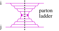
Figure 4: Cut parton ladder $G_{\mathrm{QCD}}^{\mathrm{hard,ij}}$.

Concerning the corresponding elastic scattering T-matrix, we assume

$$\boldsymbol{\boldsymbol{\mathrm{T}}}_{\mathrm{hard}}^{ij}(Q_{1}^{2},Q_{2}^{2},s,t)=i\,s\,\sigma_{\mathrm{hard}}^{ij}(Q_{1}^{2},Q_{2}^{2},s)\times\exp(R_{\mathrm{hard}}^{2}t),$$ (10)

with $R_{\mathrm{hard}}^{2}\approx 0$ [9], which is compatible with the usual relation $\sigma_{\mathrm{hard}}^{ij}=2\mathrm{Im}\,\boldsymbol{\mathrm{T}}_{\mathrm{hard}}^{ij}(t=0)/(2s)$. Furthermore assuming a purely transverse momentum exchange $t=-q_{\bot}^{2}$, the Fourier transform and division by $2s$ gives

$$T_{\mathrm{hard}}^{ij}(Q_{1}^{2},Q_{2}^{2},s,b)=\frac{1}{8\pi^{2}s}\int d^{2}q_{\bot}e^{-iq_{\bot}b}\boldsymbol{\boldsymbol{\mathrm{T}}}_{\mathrm{hard}}^{ij}(s,t)$$ (11)

$$=\frac{i}{2}\sigma_{\mathrm{hard}}^{ij}(Q_{1}^{2},Q_{2}^{2},s)\,\frac{1}{4\pi R_{\mathrm{hard}}^{2}}\exp\left(-\frac{b^{2}}{4R_{\mathrm{hard}}^{2}}\right).$$ (12)

For the corresponding $G=\mathrm{cut}\,T_{\mathrm{hard}}=2\mathrm{Im}\,T_{\mathrm{hard}}$, we get

$$G_{\mathrm{QCD}}^{\mathrm{hard,ij}}(Q_{1}^{2},Q_{2}^{2},s,b)$$ (13)

$$=\sigma_{\mathrm{hard}}^{ij}(Q_{1}^{2},Q_{2}^{2},s)\,\frac{1}{4\pi R_{\mathrm{hard}}^{2}}\exp\left(-\frac{b^{2}}{4R_{\mathrm{hard}}^{2}}\right).$$

So the cut parton ladder expression $G$ is simply the product of the dijet production cross section $\sigma_{\mathrm{hard}}^{ij}$ times a Gaussian impact parameter dependence.

2.3 Relating $\boldsymbol{\boldsymbol{G_{\mathrm{QCD}}^{\mathrm{val-val}}}}$ to the parton-parton cross section $\boldsymbol{\boldsymbol{\sigma_{\mathrm{hard}}^{ij}}}$

Here we consider the “val-val” contribution, where on both sides a valence quark is the first perturbative parton. We might imagine in the multiple Pomeron formula (as Eq. (1), but using $\boldsymbol{\mathrm{T}}$ and not $T$) for each “val-val” Pomeron an expression like

$$\sum_{i,j}\int\frac{dz^{+}dz^{-}}{z^{+}z^{-}}\boldsymbol{\mathrm{T}}_{\mathrm{hard}}^{ij}(...,z^{+}z^{-}s,...)F^{i}(z^{+})F^{j}(z^{-}),$$ (14)

where the indices $i$ and $j$ refer to the flavors of the valence quarks, with some “vertex functions” $F^{a}$, and with $s$ being the proton-proton squared cms energy.

However, the external legs of our Pomerons should always be colorless objects, carrying light-cone momentum fractions $x^{+}$on the projectile and $x^{-}$ on the target side. So each valence quark has a partner (antiquark or diquark), with the valence quark carrying a light-cone momentum fraction $z^{\pm}$ and its partner $x^{\pm}-z^{\pm}$, the sum of both being $x^{\pm}.$ The partner is emitted (as a timelike parton) immediately, and the valence quark starts the parton evolution. The corresponding cut diagram is indicated in Fig. 5.

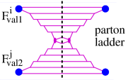
Figure 5: The contribution $G_{\mathrm{QCD}}^{\mathrm{val-val}}$ .

We imagine vertex functions $F_{\mathrm{val}\,1}^{i}$ and $F_{\mathrm{val}\,2}^{j}$ with three arguments each: the light-cone momentum fractions of the valence quark and of its partner, and the Mandelstam $t$. Let us first look at the T-matrix. Instead of Eq. (14), we use for each “val-val” Pomeron an expression (including integration) like

$$\sum_{i,j}\int\frac{dz^{+}dz^{-}}{z^{+}z^{-}}\int dx^{+}dx^{-}\boldsymbol{\mathrm{T}}_{\mathrm{hard}}^{ij}(Q_{0}^{2},Q_{0}^{2},z^{+}z^{-}s,t)$$

$$\qquad\qquad F_{\mathrm{val}\,1}^{i}(z^{+},x^{+}-z^{+},t)F_{\mathrm{val}\,2}^{j}(z^{-},x^{-}-z^{-},t),$$ (15)

which can then be written as an integration $\int dx^{+}dx^{-}/(x^{+}x^{-})$ referring to the “white” legs, with an integrand that can be interpreted as the corresponding T-matrix, i.e.

$$\int\frac{dx^{+}dx^{-}}{x^{+}x^{-}}\mathrm{\mathbf{T}}_{\mathrm{val}-\mathrm{val}}\!\left(x^{+},x^{-},s,t\right),$$ (16)

with the “val-val” T-matrix

$$\mathrm{\mathbf{T}}_{\mathrm{val}-\mathrm{val}}\!\left(x^{+},x^{-},s,t\right)$$ (17)

$$=\sum_{i,j}\int\!\!\!dz^{+}dz^{-}\frac{x^{+}x^{-}}{z^{+}z^{-}}\>\mathrm{\mathbf{T}}_{\mathrm{hard}}^{ij}\left(Q_{0}^{2},Q_{0}^{2},z^{+}z^{-}s,t\right)$$

$$\qquad F_{\mathrm{val}\,1}^{i}(z^{+},x^{+}-z^{+},t)\;F_{\mathrm{val}\,2}^{j}(z^{-},x^{-}-z^{-},t).$$

For $F_{\mathrm{val}\,1}^{i}$, $F_{\mathrm{val}\,2}^{j}$, and $\mathrm{\mathbf{T}}_{\mathrm{hard}}^{ij}$, the $t$ dependence can be factored out as $e^{R^{2}t},$ with parameters $R_{\mathrm{val}\,1}^{2}$, $R_{\mathrm{val}\,2}^{2}$, and $R_{\mathrm{hard}}^{2}$. We compute $G$ as usual as twice the imaginary part of the Fourier transform of the T-matrix divided by $2sx^{+}x^{-}$, and we get (using Eqs. (11,12) with $z^{+}z^{-}s$ instead of $s$)
$\displaystyle G_{\mathrm{QCD}}^{\mathrm{val}-\mathrm{val}}(x^{+},x^{-},s,b)=\sum_{i,j}\int dz^{+}dz^{-}$ (18) $\displaystyle\quad F_{\mathrm{val}\,1}^{i}(z^{+},x^{+}-z^{+},0)\,F_{\mathrm{val}\,2}^{j}(z^{-},x^{-}-z^{-},0)$ $\displaystyle\quad\sigma_{\mathrm{hard}}^{ij}\!\left(Q_{0}^{2},Q_{0}^{2},z^{+}z^{-}s\right)\,\frac{1}{4\pi R^{2}}\exp\!\left(-\frac{b^{2}}{4R^{2}}\right)$
with

$$R^{2}=R_{\mathrm{hard}}^{2}+R_{\mathrm{val}\,1}^{2}+R_{\mathrm{val}\,2}^{2}.$$ (19)

2.4 Relating $\boldsymbol{\boldsymbol{G_{\mathrm{QCD}}^{\mathrm{sea-sea}}}}$ to the parton-parton cross section $\boldsymbol{\boldsymbol{\sigma_{\mathrm{hard}}^{ij}}}$

For the “sea-sea” contribution, we expect a “soft block” preceding the first pertubative parton, as indicated in Fig. 6.

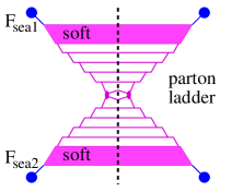
Figure 6: The contribution $G_{\mathrm{QCD}}^{\mathrm{sea-sea}}$ .

The vertices $F_{\text{sea}\,1}$ and $F_{\text{sea}\,2}$ couple the parton ladder to the projectile and target nucleons. In addition, we have three blocks, the two soft blocks and in between the parton ladder discussed earlier. The corresponding elastic scattering T-matrix for the latter is $\boldsymbol{\boldsymbol{\mathrm{T}}}_{\mathrm{hard}}^{jk}$ and those for the soft blocks are per definition $\boldsymbol{\boldsymbol{\mathrm{T}}}_{\mathrm{soft}}^{j}$ and $\boldsymbol{\boldsymbol{\mathrm{T}}}_{\mathrm{soft}}^{k}$, with $j$ and $k$ being the flavors of the two parton which connect the soft blocks to the parton ladder. In principle we have for each of these partons a four-dimensional loop integral, but based on the assumption that transverse momenta and virtualities are negligible compared to longitudinal momenta, they can be reduced to one-dimensional integrals [11],

$$i\boldsymbol{\boldsymbol{\mathrm{T}}}_{\mathrm{sea-sea}}(Q_{1}^{2},Q_{2}^{2},x^{+},x^{-},s,t)$$

$$=\sum_{ij}\int\!\frac{dz^{+}}{z^{+}}\frac{dz^{-}}{z^{-}}\mathrm{Im}\,\boldsymbol{\boldsymbol{\mathrm{T}}}_{\mathrm{soft}}^{i}\!\!\left(Q_{1}^{2},\frac{s_{0}}{z^{+}},t\right)\,\mathrm{Im}\,\boldsymbol{\boldsymbol{\mathrm{T}}}_{\mathrm{soft}}^{j}\!\!\left(Q_{2}^{2},\frac{s_{0}}{z^{-}},t\right)$$

$$\qquad i\boldsymbol{\boldsymbol{\mathrm{T}}}_{\mathrm{hard}}^{ij}(Q_{1}^{2},Q_{2}^{2},z^{+}z^{-}x^{+}x^{-}s,t)F_{\mathrm{sea\,1}}(x^{+},t)\;F_{\mathrm{sea}\,2}(x^{-},t)$$ (20)

What is the reason for getting the imaginary part of the soft T-matrices? The loop integrals may be written as $\int dk^{+}dk^{-}d^{2}k_{t}...$, and the $k^{-}$ variable can be related to the Mandelstam variables $s$ and $u$ (for the soft block). Then the usual branch cuts translate into cuts for $k^{-}$, and a rotation of the integration path,

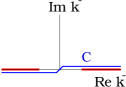
$\mathbf{\mathbf{\to}}$

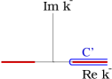
Figure 7: The integration path in the $k^{-}$ plane.

as shown in Fig. 7, transforms $\int_{-\infty}^{\infty}dk^{-}...$ into $\int_{0}^{\infty}dk^{-}\mathrm{disc}...$ which is equal to $\int_{0}^{\infty}dk^{-}\mathrm{Im}...$ . In order to compute

$$G_{\mathrm{QCD}}^{\mathrm{sea-sea}}(Q_{1}^{2},Q_{2}^{2},x^{+},x^{-},s,b)$$ (21)

$$\qquad=2\mathrm{Im}\,T_{\mathrm{sea-sea}}(Q_{1}^{2},Q_{2}^{2},x^{+},x^{-},s,b),$$

with as usual $T$ being the Fourier transform divided by $2\hat{s}=2x^{+}x^{-}s$ of the T-matrix,

$$T_{\mathrm{sea-sea}}(Q_{1}^{2},Q_{2}^{2},x^{+},x^{-},s,b)=\frac{1}{8\pi^{2}x^{+}x^{-}s}$$ (22)

$$\quad\int d^{2}q_{\bot}e^{-iq_{\bot}b}\boldsymbol{\boldsymbol{\mathrm{T}}}_{\mathrm{sea-sea}}(Q_{1}^{2},Q_{2}^{2},x^{+},x^{-},s,t),$$

we note that for all T-matrices, the $t$ dependence can be factored out as

$$\boldsymbol{\boldsymbol{\mathrm{T}}}_{\mathrm{soft}}^{i}\!\!\left(...,t\right)=\boldsymbol{\boldsymbol{\mathrm{T}}}_{\mathrm{soft}}^{i}\!\!\left(...,0\right)\times\exp\left(\left(R_{\mathrm{soft}}^{2}+\alpha^{\prime}\ln(\hat{s})\right)\,t\right),$$ (23)

$$\boldsymbol{\boldsymbol{\mathrm{T}}}_{\mathrm{hard}}^{ij}(...,t)=\boldsymbol{\boldsymbol{\mathrm{T}}}_{\mathrm{hard}}^{ij}(...,0)\times\exp\left(R_{\mathrm{hard}}^{2}\,t\right).$$ (24)

The $t$ dependence of $F_{\mathrm{sea}\,1}$ and $F_{\mathrm{sea}\,2}$ can also be factored out as $e^{R_{\mathrm{sea}\,K}^{2}t},$ with parameters $R_{\mathrm{sea}\,1}^{2}$, $R_{\mathrm{sea}\,2}^{2}$, which gives a simple overall $t$ dependence of the r.h.s of Eq. (20) as $e^{R^{2}t}$, so that we get easily

$$G_{\mathrm{sea-sea}}(Q_{1}^{2},Q_{2}^{2},x^{+},x^{-},s,b)=\sum_{ij}\int\!dz^{+}dz^{-}$$

$$\qquad\mathrm{Im}\,\boldsymbol{\boldsymbol{\mathrm{T}}}_{\mathrm{soft}}^{i}\!\!\left(Q_{1}^{2},\frac{s_{0}}{z^{+}},0\right)\mathrm{Im}\,\boldsymbol{\boldsymbol{\mathrm{T}}}_{\mathrm{soft}}^{j}\!\!\left(Q_{2}^{2},\frac{s_{0}}{z^{-}},0\right)$$ (25)

$$\qquad\frac{1}{z^{+}z^{-}x^{+}x^{-}s}\mathrm{Im}\boldsymbol{\boldsymbol{\mathrm{T}}}_{\mathrm{hard}}^{ij}(Q_{1}^{2},Q_{2}^{2},z^{+}z^{-}x^{+}x^{-}s,0)$$

$$\qquad F_{\mathrm{sea\,1}}(x^{+},0)\;F_{\mathrm{sea}\,2}(x^{-},0)\>\frac{1}{4\pi R^{2}}\exp\left(-\frac{b^{2}}{4R^{2}}\right).$$

Using

$$\frac{1}{\hat{s}}\mathrm{Im}\boldsymbol{\boldsymbol{\mathrm{T}}}_{\mathrm{hard}}^{ij}(Q_{1}^{2},Q_{2}^{2},\hat{s},0)=\sigma_{\mathrm{hard}}^{ij}(Q_{1}^{2},Q_{2}^{2},\hat{s}),$$ (26)

and defining so-called “soft evolution functions”

$$E_{\mathrm{soft}}^{i}(Q^{2},z)=\mathrm{Im}\,\boldsymbol{\boldsymbol{\mathrm{T}}}_{\mathrm{soft}}^{i}\!\!\left(Q^{2},\frac{s_{0}}{z},0\right),$$ (27)

we get finally
$\displaystyle G_{\mathrm{QCD}}^{\mathrm{sea-sea}}(Q_{1}^{2},Q_{2}^{2},x^{+},x^{-},s,b)=\sum_{ij}\int\!dz^{+}dz^{-}$ (28) $\displaystyle\qquad\quad F_{\mathrm{sea\,1}}(x^{+},0)\,F_{\mathrm{sea}\,2}(x^{-},0)\,E_{\mathrm{soft}}^{i}(Q_{1}^{2},z^{+})E_{\mathrm{soft}}^{j}(Q_{2}^{2},z^{-})$ $\displaystyle\qquad\quad\sigma_{\mathrm{hard}}^{ij}(Q_{1}^{2},Q_{2}^{2},z^{+}z^{-}x^{+}x^{-}s)\,\frac{1}{4\pi R^{2}}\exp\left(-\frac{b^{2}}{4R^{2}}\right),$
with $R$ being given explicitly as

$$R^{2}=R_{\mathrm{sea}\,1}^{\,2}+R_{\mathrm{sea}\,2}^{\,2}+2R_{\mathrm{soft}}^{2}+\alpha^{\prime}\ln(\frac{1}{z^{+}})+\alpha^{\prime}\ln(\frac{1}{z^{-}})+R_{\mathrm{hard}}^{2}.$$ (29)

The precise form of $E_{\mathrm{soft}}^{i}$ and $F_{\mathrm{sea}\,K}$ will be discussed later, the former is based on a parametrization (in Regge-pole form) of the soft T-matrix, the latter has a simple power law form.

2.5 Relating $\boldsymbol{\boldsymbol{G_{\mathrm{QCD}}^{\mathrm{val-sea}}}}$ and $\boldsymbol{\boldsymbol{G_{\mathrm{QCD}}^{\mathrm{sea-val}}}}$ to the parton-parton cross section $\boldsymbol{\boldsymbol{\sigma_{\mathrm{hard}}^{ij}}}$

Having discussed the two contributions “val-val” and “sea-sea”, referring to contributions with respectively two valence quarks and two sea quarks as “first perturbative partons” entering the parton ladder, we easily obtain the expressions for “val-sea”, namely
$\displaystyle G_{\mathrm{QCD}}^{\mathrm{val}-\mathrm{sea}}(Q_{2}^{2},x^{+},x^{-},s,b)=\sum_{i,j}\int dz^{+}dz^{-}$ (30) $\displaystyle\quad F_{\mathrm{val}\,1}^{i}(z^{+},x^{+}-z^{+},0)\,F_{\mathrm{sea}\,2}(x^{-},0)\,E_{\mathrm{soft}}^{j}(Q_{2}^{2},z^{-})$ $\displaystyle\quad\sigma_{\mathrm{hard}}^{ij}\!\left(Q_{0}^{2},Q_{2}^{2},z^{+}z^{-}x^{-}s\right)\,\frac{1}{4\pi R^{2}}\exp\!\left(-\frac{b^{2}}{4R^{2}}\right),$
with $R$ being given explicitly as

$$R^{2}=R_{\mathrm{val}\,1}^{2}+R_{\mathrm{sea}\,2}^{\,2}+R_{\mathrm{soft}}^{2}+\alpha^{\prime}\ln(\frac{1}{z^{-}})+R_{\mathrm{hard}}^{2}.$$ (31)

The expression for “sea-val” is
$\displaystyle G_{\mathrm{QCD}}^{\mathrm{sea}-\mathrm{val}}(Q_{1}^{2},x^{+},x^{-},s,b)=\sum_{i,j}\int dz^{+}dz^{-}$ (32) $\displaystyle\quad F_{\mathrm{sea\,1}}(x^{+},0)\,E_{\mathrm{soft}}^{i}(Q_{1}^{2},z^{+})\,F_{\mathrm{val}\,2}^{j}(z^{-},x^{-}-z^{-},0)$ $\displaystyle\quad\sigma_{\mathrm{hard}}^{ij}\!\left(Q_{1}^{2},Q_{0}^{2},z^{+}z^{-}x^{+}s\right)\,\frac{1}{4\pi R^{2}}\exp\!\left(-\frac{b^{2}}{4R^{2}}\right),$
with $R$ being given explicitly as

$$R^{2}=R_{\mathrm{sea}\,1}^{\,2}+R_{\mathrm{soft}}^{2}+\alpha^{\prime}\ln(\frac{1}{z^{+}})+R_{\mathrm{val}\,2}^{2}+R_{\mathrm{hard}}^{2}.$$ (33)

2.6 The vertices F

The main formulas of the preceding sections, Eqs. (18,28,30,32), allow to express the different $G_{\mathrm{QCD}}^{J}$ in terms of “modules”, among them the vertices $F_{\mathrm{sea}\,K}$ and $F_{\mathrm{val}\,K}$ with $K\in\{1,2\}$, which are simple functions, to be discussed in the following. In the case of pp scattering, the functions for $K=1$ and $K=2$ are identical, whereas for $\pi$p or Kp scattering they are in general different (more precisely, the form is the same but not the parameters). The vertices $F_{\mathrm{sea}\,K}$ and $F_{\mathrm{val}\,K}^{i}$ are given as
$\displaystyle F_{\mathrm{sea}\,K}(x)$ $\displaystyle=\gamma_{\mathrm{sea}\,K}\,\,x^{-\alpha_{\mathrm{sea}\,K}},$ (34) $\displaystyle F_{\mathrm{val}\,K}^{i}(z,z^{\prime})$ $\displaystyle=N^{-1}\,q_{\mathrm{val}}^{i}(z)(1-z)^{\alpha_{\mathrm{I}\!\mathrm{R}}-1-\alpha_{\mathrm{remn}}}z^{\prime}{}^{-\alpha_{\mathrm{I}\!\mathrm{R}}},$ (35)
with $N=\Gamma\!\left(1+\alpha_{\mathrm{remn}}\right)\,\Gamma\!\left(1-\alpha_{\mathrm{I}\!\mathrm{R}}\right)/\Gamma\!\left(2+\alpha_{\mathrm{remn}}-\alpha_{\mathrm{I}\!\mathrm{R}}\right)$, with $q_{\mathrm{val}}^{i}$ being a standard valence quark distribution function for a small value $Q_{0}^{2}$ of the virtuality (see [11] Appendix C.2). From Eq. (35), and using $V(z)=z^{\alpha_{\mathrm{remn}}}$ as remnant vertex, we obtain as parton distribution $f^{i}$ at $Q_{0}^{2}$

$$f^{i}(z)=\int_{0}^{1-z}dz^{\prime}\,F_{\mathrm{val}}^{i}(z,z^{\prime})\,V(1-z-z^{\prime})=q_{\mathrm{val}}^{i}(z),$$ (36)

having used $\int_{0}^{1}dy\,y{}^{-\alpha_{\mathrm{I}\!\mathrm{R}}}\,(1-y)^{\alpha_{\mathrm{remn}}}=$$\frac{\Gamma(1-\alpha_{\mathrm{I}\!\mathrm{R}})\Gamma(1+\alpha_{\mathrm{remn}})}{\Gamma(2-\alpha_{\mathrm{I}\!\mathrm{R}}+\alpha_{\mathrm{remn}})}$. So we get $f^{i}(z)=q_{\mathrm{val}}^{i}(z)$, as it should be, which justifies our choice of $F_{\mathrm{val}\,K}^{i}$.

2.7 The soft elements E_soft and G_soft

Based on the asymptotic Regge-pole expression, the soft T-matrix $\boldsymbol{\mathrm{T}}_{\mathrm{soft}}^{i}(Q^{2},s,t)$ is (for the moment) assumed to not depend on $Q^{2}$ and to be proportional to to $i\,s^{1+B_{\mathrm{soft}}}\exp\left((2R_{\mathrm{soft}}^{2}+\alpha^{\prime}\ln\frac{s}{s_{0}})t\right)$, with a “Regge-pole intercept” $1+B_{\mathrm{soft}}=\alpha_{\mathrm{soft}}(0)$, where $B_{\mathrm{soft}}$ is a parameter close to zero. The “soft evolution functions” $E_{\mathrm{soft}}^{i}(Q^{2},z)$ are defined in Eq. (27) as the imaginary part of $\boldsymbol{\mathrm{T}}_{\mathrm{soft}}^{i}$ for $t=0$ and $s=s_{0}/z$, so they are up to constants equal to $(s_{0}/z)^{1+B_{\mathrm{soft}}}$. We add a splitting into a quark, as well as a soft-Pomeron-ladder coupling of the form $(1-z)^{C_{\mathrm{soft}}}$, to get (we drop the $Q^{2}$ argument)
$\displaystyle E_{\mathrm{soft}}^{g}\left(z\right)=\left(1-w_{\mathrm{split}}\right)\,E_{\mathrm{soft}}\left(z\right),$ (37) $\displaystyle E_{\mathrm{soft}}^{q}\left(z\right)=w_{\mathrm{split}}\,\int_{z}^{1}\!d\xi\,f_{\mathrm{split}}(\xi)\,E_{\mathrm{soft}}\left(\frac{z}{\xi}\right),$ (38) $\displaystyle\mathrm{with}\,E_{\mathrm{soft}}\left(z\right)=A_{\mathrm{soft}}\,z^{-1-B_{\mathrm{soft}}}\,(1-z)^{C_{\mathrm{soft}}},$ (39)
with a parameter $w_{\mathrm{split}}\in[0,1]$, and where we use $f_{\mathrm{split}}(\xi)=P_{g}^{q}(\xi)$, since we are “close to the perturbative domain”.

Still based on the soft T-matrix expression $\propto i\,s^{1+B_{\mathrm{soft}}}\exp\left((2R_{\mathrm{soft}}^{2}+\alpha^{\prime}\ln\frac{s}{s_{0}})t\right)$ and adding the same two vertices as for the “sea-sea” contribution, we get the “soft” $G$ expressions as

$\displaystyle G_{\mathrm{soft}}(x^{+},x^{-},s,b)=$ (40) $\displaystyle\qquad\quad F_{\mathrm{sea\,1}}(x^{+},0)\,F_{\mathrm{sea}\,2}(x^{-},0)$ $\displaystyle\qquad\quad D{}_{\mathrm{soft}}\times(x^{+}x^{-}s){}^{B_{\mathrm{soft}}}\,\frac{1}{4\pi R^{2}}\exp\left(-\frac{b^{2}}{4R^{2}}\right),$
with parameters $D_{\mathrm{soft}}$ and $B_{\mathrm{soft}}$, and with $R$ being given explicitly as

$$R^{2}=R_{\mathrm{sea}\,1}^{\,2}+R_{\mathrm{sea}\,2}^{\,2}+2R_{\mathrm{soft}}^{2}+\alpha^{\prime}\ln(\frac{s}{s_{0}}).$$ (41)

2.8 The pseudosoft elements E_psoft and G_psoft

The “soft evolution functions” $E_{\mathrm{soft}}^{i}$ are meant to take care of the “non-perturbative part”, before entering the perturbative regime represented by $E_{\mathrm{QCD}}^{ik}(x,Q^{2},\mu_{\mathrm{F}}^{2})$. Originally, we were using $Q^{2}$ being equal to some soft scale $Q_{0}^{2}$ (typically $1-2\,\mathrm{GeV}^{2}$). In that case, $E_{\mathrm{soft}}^{i}$ represents purely soft physics, and we could actually drop $Q^{2}$ as an argument, $E_{\mathrm{soft}}^{i}=E_{\mathrm{soft}}^{i}(z)$. However, now we introduce evolution functions $E_{\mathrm{QCD}}^{ik}(x,Q_{\mathrm{sat}}^{2},\mu_{\mathrm{F}}^{2})$ where the virtuality cutoff is equal to the saturation scale, which is in general bigger than $Q_{0}^{2}$, which means that the “part not taken care of” by the QCD evolution, is not purely soft anymore. This is the domain of gluon fusions, but there should be emissions as well and a narrowing of the momentum fraction distributions. To take this into account we define “pseudosoft evolution functions” as

$\displaystyle E_{\mathrm{psoft}}^{k}(Q_{\mathrm{sat}}^{2},\xi)$ (42) $\displaystyle=\int dz\,dy\Big{\{}\sum_{i}E_{\mathrm{soft}}^{i}(z)E_{\mathrm{QCD}}^{ik}(y,Q_{0}^{2},Q_{\mathrm{sat}}^{2})\delta(\xi-zy)\Big{\}},$

which is meant to replace the soft evolution functions used so far. This is actually needed to have the same $p_{t}$ distribution of emitted partons at large $p_{t}$ for different values of $Q_{\mathrm{sat}}^{2}$.

Having replaced the soft evolution functions with the pseudosoft ones, we need a modification of $G_{\mathrm{soft}}$ as well. We have little guidance from theory, so we use the same parametrization as for $G_{\mathrm{soft}}$

$\displaystyle G_{\mathrm{psoft}}(Q_{\mathrm{sat}}^{2},x^{+},x^{-},s,b)=$ (43) $\displaystyle\qquad\quad F_{\mathrm{sea\,1}}(x^{+},0)\,F_{\mathrm{sea}\,2}(x^{-},0)$ $\displaystyle\qquad\quad D{}_{\mathrm{psoft}}\times(x^{+}x^{-}s){}^{B_{\mathrm{psoft}}}\,\frac{1}{4\pi R^{2}}\exp\left(-\frac{b^{2}}{4R^{2}}\right),$
just with different parameters $B_{\mathrm{psoft}}$ and $D_{\mathrm{psoft}}$, which may depend on $Q_{\mathrm{sat}}^{2}$. This is enough to compute $G_{\mathrm{QCD}}$. But because of $Q_{\mathrm{sat}}^{2}>Q_{0}^{2}$, we expect that hard pQCD processes should occur, producing light and heavy flavor hadrons. This will be discussed more in the next section.

3 Parton-parton cross sections in EPOS4 involving light and heavy flavors

As discussed in section 1 (see also [6]), the multiple scattering contributions to the total cross section are expressed in terms of (products of) cut Pomeron expressions $G$, each one representing a single scattering. They are related to the “real QCD expressions” $G_{\mathrm{QCD}}$ via Eq. (6), in other words, $G_{\mathrm{QCD}}$ is the fundamental building block of the multiple scattering framework of EPOS4. We showed in section 2, that $G_{\mathrm{QCD}}$ has several contributions, each one being composed of “modules”, with the “key” module being the integrated inclusive parton-parton scattering cross section $\sigma_{\mathrm{hard}}^{ij}$, where $i$ and $j$ refer to the flavors of the two partons. This “module” $\sigma_{\mathrm{hard}}^{ij}$ contains all the pQCD calculations. We refer to Table 1 in section 2 to recall the definitions of the symbols $G$ and $\sigma$ and their relation to the T-matrix. In this section, we discuss in detail how to compute $\sigma_{\mathrm{hard}}^{ij}$.

Concerning notations: whereas in the previous section the symbol $s$ usually referred to the Mandestam $s$ of nucleon-nucleon scattering, we will use in this section $s$ and $t$ referring to the Born process of the hard scattering, which here plays a crucial role. Although it is not always explicitly written, the pQCD matrix elements $\mathcal{M}$ are always considered to be given in term of $s$ and $t$ (that is how the are tabulated).

3.1 Integrated and differential partonic cross sections

The main formula concerning the parton-parton scattering cross section $\sigma_{\mathrm{hard}}^{ij}$ is Eq. (9). It is useful to split that formula, by first considering “differential cross sections”

$$E_{3}E_{4}\frac{d^{6}\sigma_{\mathrm{hard}}^{ij}}{d^{3}p_{3}d^{3}p_{4}}=\sum_{klmn}\int\!\int\!\!dx_{1}dx_{2}$$ (44)

$$\qquad\,E_{\mathrm{QCD}}^{ik}(x_{1},Q_{1}^{2},\mu_{\mathrm{F}}^{2})E_{\mathrm{QCD}}^{jl}(x_{2},Q_{2}^{2},\mu_{\mathrm{F}}^{2})$$

$$\qquad\frac{1}{32s\pi^{2}}\bar{\sum}|\mathcal{M}^{kl\to mn}|^{2}\delta^{4}(p_{1}+p_{2}-p_{3}-p_{4})\frac{1}{1+\delta_{mn}},$$

representing the inelastic scattering of two partons with virtualities $Q_{1}^{2}$ and $Q_{2}^{2}$ at a center-of-mass energy squared $s_{\mathrm{lad}}$, with $x_{1/2}$ being the light-cone (LC) momentum fractions (with respect to the LC momenta of the partons before the evolution) of the partons entering the Born process of the elementary parton-parton scattering $1+2\to 3+4$, see Fig. 8,

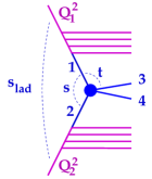
Figure 8: The differential parton-parton cross section $E_{3}E_{4}d^{6}\sigma_{\mathrm{hard}}^{ij}/d^{3}p_{3}d^{3}p_{4}$ considering the Born process $1+2\to 3+4$. The solid lines represent partons (quarks, antiquarks, or gluons).

with the corresponding flavors $k$, $l$, $m$ and $n$. The matrix elements $\mathcal{M}$ is considered to be given in term of $s$ and $t$, with $s=x_{1}x_{2}s_{\mathrm{lad}}$. Both partons first evolve via parton emissions with ordered virtualities up to $\mu_{F}^{2}$ before interacting as an elementary $2\to 2$ pQCD scattering. The “integrated cross sections” $\sigma_{\mathrm{hard}}^{ij}$ may then be written as

$$\sigma_{\mathrm{hard}}^{ij}(s_{\mathrm{lad}},Q_{1}^{2},Q_{2}^{2})\!=\!\int\frac{d^{3}p_{3}d^{3}p_{4}}{E_{3}E_{4}}\left\{E_{3}E_{4}\frac{d^{6}\sigma_{\mathrm{hard}}^{ij}}{d^{3}p_{3}d^{3}p_{4}}\right\},$$ (45)

in terms of the “differential cross section”. Both differential and integrated cross sections are important in the EPOS4 framework:

• the integrated ones are needed to compute the weights for all possible parallel scattering configurations, and to generate the corresponding configurations,

• the differential cross sections are needed to compute parton distributions, and generate partons in the Monte Carlo mode, for given configurations (generated in the first step).

Comparing Eq. (8) and Eq. (44), we see that our differential cross section has the same structure as the inclusive cross section based on factorization, but in our case, we use evolution functions $E_{\mathrm{QCD}}$ rather than the usual parton distribution functions $f_{\mathrm{PDF}}$, where $E_{\mathrm{QCD}}$ represents an evolution also according to DGLAP [9, 12, 13], but starting from a parton and not from a proton, with an initial condition $E_{\mathrm{QCD}}^{ik}(z,Q_{1}^{2},Q_{1}^{2})=\delta_{ik}\;\delta(1-z)$. Special care is needed to treat this “singularity”.

We will eventually use dynamical saturation scales $Q_{\mathrm{sat\,1}}^{2}$ and $Q_{\mathrm{sat\,2}}^{2}$ as endpoint virtualities, so we compute (via numerical integration) and then tabulate $\sigma_{\mathrm{hard}}^{ij}(s_{\mathrm{lad}},Q_{1}^{2},Q_{2}^{2})$ for a large range of possible values $s_{\mathrm{lad}}$, $Q_{1}^{2}$, and $Q_{2}^{2}$ for all possible combinations of $i$ and $j$. During the simulations, we use the predefined tables to compute $\sigma_{\mathrm{hard}}^{ij}$ via polynomial interpolation.

As discussed in detail later, all the kinematic variables shown in fig. 8 are related to each other: The scale $\mu_{\mathrm{F}}^{2}$ and the Mandelstam variable $t$ are related to $p_{t}^{2}$ (the transverse momentum of one of the outgoing partons, say parton 3), the end virtualities $Q_{1}^{2}$ and $Q_{2}^{2}$ represent lower limits to $p_{t}^{2}$, but the precise relations depend on the particular Born process. We deal with this problem by introducing classes of cross sections, with the same Born kinematics per class. The main reason that we need to be very careful concerning parton kinematics is the fact that in our case, the differential cross section formula Eq. (44) concerns one single scattering in a multiple scattering configuration as shown in Fig. 9.

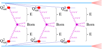
Figure 9: Multiple scattering configuration for three scatterings.

Here we show an example with three scatterings, but in AA collisions, we have configurations with 1000 scatterings. So it is out of question to use the standard method of Monte Carlo programming, namely rejection in the case of forbidden kinematics, we simply have to avoid such cases.

3.2 Parton evolution functions $\boldsymbol{\boldsymbol{E_{\mathrm{QCD}}}}$

Our parton evolution functions $E_{\mathrm{QCD}}^{ik}$ are similar to the “usual” ones, obeying the same evolution equations, but the initial conditions are different, and this requires different treatments. We present here a new procedure to compute and tabulate these functions, much faster than the techniques we used in EPOS3. The indices $i$ and $k$ refer to parton flavors in the form of integers with $0$ for a gluon, $1-6$ for quark flavors from $u$ to $t$, and the corresponding negative numbers for the antiquarks.

For a given end parton $i$, using $t=Q^{2}$, the evolution equation for an evolution from $t_{a}$ to $t_{b}$ may be written as [2]

$$E_{\mathrm{QCD}}^{ik}\left(x,t_{a},t_{b}\right)=\Delta^{i}(t_{a},t_{b})\delta(1-x)\delta_{ik}$$ (46)

$$\qquad+\sum_{j}\int\frac{dt}{t}\int\frac{dz}{z}\,E_{\mathrm{QCD}}^{ij}\left(\frac{x}{z},t_{a},t\right)\bar{P}_{j}^{k}\!(t,z)\,\Delta^{k}(t,t_{b})$$

with

$$t_{a}\leq t\leq t_{b},\;x\leq z\leq 1-\epsilon\>.$$ (47)

We use $\bar{P}=\frac{\alpha_{s}}{2\pi}P$, with $P$ being the splitting functions without $()_{+}$ prescription, i.e., [2]

$$P_{q}^{q}(t,z) =C_{F}\,(1+z^{2})/(1-z)\>,$$ (48)

$$P_{g}^{q}(t,z) =\theta(|q|-N_{f}(t))\,\begin{array}[]{c}\frac{1}{2}\end{array}(z^{2}+(1-z)^{2})\>,$$ (50)

$$P_{q}^{g}(t,z) =C_{F}\,(1+(1-z)^{2})/z\>,$$ (51)

$$P_{g}^{g}(t,z) =2C_{A}\,(\,z/(1-z)+(1-z)/z+z(1-z)\,)\>,$$ (52)

with quark indices $q\in\{-6,...,-1,1,...,6\}$ and $g=0$, with $C_{F}=4/3$, $T_{R}=1/2$, $C_{A}=3$, and where

$$\theta(N_{f}-|q|)=\left\{\begin{array}[]{cl}1&\mathrm{for}\>N_{f}(t)\geq|q|\\ 0&\mathrm{otherwise}\end{array}\right.$$

assures a possible emission of a quark of flavor $q$ if the number of flavors $N_{f}(t)$ is at least as big as $|q|$. So for large values of $t$, with $N_{f}(t)=5$, the weight for emitting a bottom quark is identical to the one of a $u$ or $d$ quark. The symbols $\Delta^{i}$ refer to the so-called Sudakov form factors, defined as

$$\Delta^{q}(t_{1},t_{2})=\exp\left(-\int_{t_{1}\,^{2}}^{t_{2}}\frac{dt}{t}\frac{\alpha_{s}}{2\pi}\int_{\epsilon}^{1-\epsilon}dz\,P_{q}^{q}(z)\right),$$ (53)

and

$$\;\Delta^{g}(t_{1},t_{2})=$$

$$\exp\left(\,\!-\int_{t_{1}\,^{2}}^{t_{2}}\frac{dt}{t}\frac{\alpha_{s}}{2\pi}\int_{\epsilon}^{1-\epsilon}\,\,dz\,\left(\frac{1}{2}P_{g}^{g}(z)+N_{f}P_{g}^{q}(z)\right)\right),$$ (54)

see Appendix A.3.

The fundamental difference with respect to the “usual” PDFs is the fact that we have a singular initial condition, namely

$$E_{\mathrm{QCD}}^{ab}\left(x,t_{a},t_{a}\right)=\delta(1-x)\delta_{ab},$$ (55)

so we have to define the evolution function $\widetilde{E}_{\mathrm{QCD}}^{ab}\left(x,t_{a},t_{b}\right)$ for at least one emission, such that the evolution function can be written as

$$E_{\mathrm{QCD}}^{ab}\left(x,t_{a},t_{b}\right)=\widetilde{E}_{\mathrm{QCD}}^{ab}\left(x,t_{a},t_{b}\right)+\Delta^{a}(t_{a},t_{b})\delta(1-x)\delta_{ab},$$ (56)

with $\widetilde{E}_{\mathrm{QCD}}^{ab}\left(x,t_{a},t_{a}\right)=0$. As proven in Appendix A.2, we have for an arbitrary $t_{c}$ between $t_{a}$ and $t_{b}$ the relation

$$E_{\mathrm{QCD}}^{ab}\left(x,t_{a},t_{b}\right)=\sum_{c}\int\frac{dz}{z}E_{\mathrm{QCD}}^{ac}\left(\frac{x}{z},t_{a},t_{c}\right)E_{\mathrm{QCD}}^{cb}\left(z,t_{c},t_{b}\right)\,,$$ (57)

and using Eq. (56), we get

$$\widetilde{E}_{\mathrm{QCD}}^{ab}\left(x,t_{a},t_{b}\right)=\widetilde{E}_{\mathrm{QCD}}^{ab}\left(x,t_{a},t_{c}\right)\Delta^{b}(t_{c},t_{b})\qquad\qquad$$

$$+\Delta^{a}(t_{a},t_{c})\widetilde{E}_{\mathrm{QCD}}^{ab}\left(x,t_{c},t_{b}\right)$$ (58)

$$\qquad\qquad\ +\sum_{c}\int\frac{dz}{z}\widetilde{E}_{\mathrm{QCD}}^{ac}\left(\frac{x}{z},t_{a},t_{c}\right)\widetilde{E}_{\mathrm{QCD}}^{cb}\left(z,t_{c},t_{b}\right).$$

We tabulate $\widetilde{E}$, which means we compute $\widetilde{E}_{\mathrm{QCD}}^{ab}\left(x,t_{i},t_{j}\right)$ with $t_{\min}\leq t_{i}\leq t_{j}\leq t_{\max}$ (blue area in the $t_{i}-t_{j}$ plane, in Fig. 10)

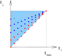
Figure 10: Tabulating the evolution function.

explicitly

$$t_{i}=t_{\mathrm{min}}\left(\frac{t_{\mathrm{max}}}{t_{\min}}\right)^{(i-1)/(M-1)},$$ (59)

and

$$t_{j}=t_{i}\left(\frac{t_{\mathrm{max}}}{t_{i}}\right)^{(j-1)/(M-1)},$$ (60)

for $i,j$ from $1$ to $M$. We first compute $\widetilde{E}_{\mathrm{QCD}}^{ab}\left(x,t_{i},t_{j}\right)$ for all $i$ and $j=1$ and $j=2$ in an iterative fashion. These are the red points in Fig. 10. We then compute the $\widetilde{E}$ values for $j=3,4,5...$, always for $i=1$ to $i=M$. We use Eq. (58) as

$$\widetilde{E}_{\mathrm{QCD}}^{ab}\left(x,t_{i},t_{j}\right)=\widetilde{E}_{\mathrm{QCD}}^{ab}\left(x,t_{i},t_{j-1}\right)\Delta^{b}(t_{j-1},t_{j})\qquad\qquad$$

$$+\Delta^{a}(t_{i},t_{j-1})\widetilde{E}_{\mathrm{QCD}}^{ab}\left(x,t_{j-1},t_{j}\right)$$ (61)

$$\qquad\qquad\ +\sum_{j-1}\int\frac{dz}{z}\widetilde{E}_{\mathrm{QCD}}^{ac}\left(\frac{x}{z},t_{i},t_{j-1}\right)\widetilde{E}_{\mathrm{QCD}}^{cb}\left(z,t_{j-1},t_{j}\right).$$

This works, since $\widetilde{E}_{\mathrm{QCD}}^{ab}\left(x,t_{i},t_{j-1}\right)$ and $\widetilde{E}_{\mathrm{QCD}}^{cb}\left(x,t_{j-1},t_{j}\right)$ are already known via interpolation from already tabulated values. In this way, we are able to compute and tabulate the evolution functions $\widetilde{E}_{\mathrm{QCD}}^{ab}$, and use them via polynomial interpolation, and thus we know $E_{\mathrm{QCD}}^{ab}$ via Eq. (56).

3.3 Computing integrated parton-parton cross sections with quark mass dependent kinematics

As discussed in the last section, the integrated parton-parton cross section $\sigma_{\mathrm{hard}}^{ij}$ is a crucial element of the EPOS4 framework. It may be written as (see Appendix B.2 Eq. (262))

$$\sigma_{\mathrm{hard}}^{ij}\!=\!\!\sum_{klmn}\int\!\!dx_{1}\,dx_{2}\,dt\,E_{\mathrm{QCD}}^{ik}(x_{1},Q_{1}^{2},\mu_{\mathrm{F}}^{2})E_{\mathrm{QCD}}^{jl}(x_{2},Q_{2}^{2},\mu_{\mathrm{F}}^{2})$$

$$\qquad\qquad\qquad\times\frac{\pi\alpha_{s}^{2}}{s^{2}}\left\{\frac{1}{g^{4}}\bar{\sum}|\mathcal{M}^{kl\to mn}|^{2}\right\}\frac{1}{1+\delta_{mn}},$$ (62)

where the indices $i$, $j$, $k$, $l$, $m$, $n$ refer to all kinds of flavors (gluons and (anti)quarks up to bottom). The matrix elements $\mathcal{M}$ is considered to be given in terms of $s$ and $t$, with $s=x_{1}x_{2}s_{\mathrm{lad}}$, with $s_{\mathrm{lad}}$ referring to the parton-parton scattering, see Fig. 8. EPOS was originally constructed only for light flavors, simply considering two types of partons, massless quarks and gluons. Very often, in the program, the two cases were simply treated explicitly, which required major changes in the code structure. For instance, the number of active flavors (which appears in $\alpha_{s}$ and the splitting function), which was a constant so far, now depends on $Q^{2}$.

And there is a second challenge: In the “massless case” of earlier versions, we could first do the sum over all Born processes and compute “the” Born cross section for a given pair of partons $k$ and $l$,

$$\sum_{mn}\left\{\frac{1}{g^{4}}\bar{\sum}|\mathcal{M}^{kl\to mn}|^{2}\right\}$$ (63)

before doing the integrals, which considerably simplifies the calculations. Now we need explicitly the information about the process $kl\to mn$, since the masses involved in the process affect the kinematics (like the relation between Mandelstam $t$ and $p_{t}$ and integration limits). So the operations $\sum_{mn}$ and $\int dx_{1}dx_{2}dt$ can no longer be exchanged in general, but it can be within classes: We introduce classes $K$ of elementary reactions $kl\to mn$ obeying to the same kinematics and then compute all relevant quantities (to be discussed in detail in the next section) depending on of $K$. In this way we do the kinematics properly and still keep efficient (fast) procedures, which is crucial in the EPOS4 framework.

3.3.1 Born kinematics

In the last section, we were considering processes involving initial partons $i$ and $j$ and two partons $k$ and $j$ entering the Born process (let us note them $1$ and $2$), producing partons $m$ and $n$ (let us note them $3$ and $4$), so altogether we have the Born process $1+2\to 3+4$. In the CMS, we write the parton momentum four-vectors as

$$p=(\sqrt{E\text{\texttwosuperior}+M\text{\texttwosuperior}},\vec{p}_{t},p_{z}),\quad\mathrm{with}\;M^{2}=p^{2},$$ (64)

with $\vec{p}_{t}=0$ for the incoming ones. So per definition, $E$ is the modulus of the momentum, $E=|\vec{p}|$, in the CMS, and so we have obviously for all four particles

$$p_{z}^{2}=E^{2}-p_{t}^{2}\>,$$ (65)

and

$$E_{1}=E_{2}\,,\;E_{3}=E_{4}.$$ (66)

In the following, $E$ (without index) refers to $E_{1}$ ($=E_{2}$) and $E^{\prime}$ to $E_{3}$ ($=E_{4}$). We will use the following definitions:

$$W=4E^{2},\;W^{\prime}=4E^{\prime 2}.$$ (67)

From energy conservation, we find

$$s=\left(\sqrt{E^{2}+m_{1}^{2}}+\sqrt{E^{2}+m_{2}^{2}}\right)^{2},$$ (68)

$$\,=\left(\sqrt{E^{\prime 2}+m_{3}^{2}}+\sqrt{E^{\prime 2}+m_{4}^{2}}\right)^{2}$$ (69)

which gives

$$W=s-2\left(m_{1}^{2}+m_{2}^{2}\right)+\frac{1}{s}\left(m_{1}^{2}-m_{2}^{2}\right)^{2},$$ (70)

$$W^{\prime}=s-2\left(m_{3}^{2}+m_{4}^{2}\right)+\frac{1}{s}\left(m_{3}^{2}-m_{4}^{2}\right)^{2}.$$ (71)

In case of $m_{1}=m_{2}=m,$ we have

$$W=s-4m^{2}.$$ (72)

In case of $m_{1}=0$, $m_{2}=m$ or $m_{1}=m$, $m_{2}=0$, we have

$$W=\frac{\left(s-m^{2}\right)^{2}}{s}\,,$$ (73)

and in case of $m_{1}=m_{2}=0$, we get

$$W=s.$$ (74)

Corresponding formulas apply for $W^{\prime}$. Essentially all kinematic relations will be expressed in terms of $W$ and $W^{\prime}$.

3.3.2 Constraints for p_t

Crucial for the following discussions is the relation between the factorization scale and the transverse momentum of the outgoing parton,

$$\mu_{\mathrm{F}}^{2}=\frac{p_{t}^{2}+\lambda M^{2}}{\kappa},$$ (75)

or it’s inverse

$$p_{t}^{2}=\kappa\mu_{\mathrm{F}}^{2}-\lambda M^{2}\equiv\Pi_{\mathrm{F}}\left(\mu_{\mathrm{F}}^{2}\right),$$ (76)

with $M$ being the (maximum) mass of the partons involved in the Born process, and where the two coefficients $\kappa$ and $\lambda$ represent the freedom in defining $\mu_{\mathrm{F}}^{2}\left(p_{t}^{2}\right)$. In EPOS4.0.0, we use $\kappa=1$ and $\lambda=0$. A choice $\kappa=1$ and $\lambda=1$ makes little difference (and only at very small $p_{t}$) for charm production, but for bottom one should better use this choice, as we will do in future releases.

The $p_{t}^{2}$ values in the integration in the cross section formulas of the last section are restricted, since we have

$$\mu_{\mathrm{F}}^{2}\geq\max\!\left[Q_{1}^{2},Q_{2}^{2}\right],$$ (77)

which amounts to

$$p_{t}^{2}\geq p_{t\,\min}^{2}=\Pi_{\mathrm{F}}(\max\!\left[Q_{1}^{2},Q_{2}^{2}\right]).$$ (78)

In reality, we have to use the Mandelstam $t$ rather than $p_{\bot}^{2}$ in the integration, so we need to find the limits for this variable.

3.3.3 Constraints for s

The quantity $E^{\prime}$ is precisely the upper limit for the transverse momentum of particle $3$, i.e.,

$$p_{t}^{2}\leq p_{t\,\mathrm{max}}^{2}=E^{\prime 2}=\frac{W^{\prime}}{4}.$$ (79)

To get non-zero results, we need

$$p_{t\,\mathrm{min}}^{2}<p_{t\,\mathrm{max}}^{2}=E^{\prime 2}=\frac{W^{\prime}}{4}.$$ (80)

which gives

$$W^{\prime}=s-2\left(m_{3}^{2}+m_{4}^{2}\right)+\frac{1}{s}\left(m_{3}^{2}-m_{4}^{2}\right)^{2}>4p_{t\,\mathrm{min}}^{2},$$ (81)

and solving the quadratic inequality equation, we get

$$s_{\min}=d\Big{(}1+\sqrt{1-\left((m_{3}^{2}-m_{4}^{2})/d\right)^{2}}\Big{)}\;$$ (82)

$$\mathrm{with}\quad d=m_{3}^{2}+m_{4}^{2}+2\,p_{t\,\mathrm{min}}^{2}.$$

This is first of all a limit for the energy squared of the Born process, but of course as well a limit for the ladder.

3.3.4 Constraints for t

Concerning $t$, we have

$$t=\left(\sqrt{E^{\prime 2}+m_{3}^{2}}-\sqrt{E^{2}+m_{1}^{2}}\right)^{2}$$

$$\qquad\qquad-\left(\vec{p}_{t}-\vec{0}\right)^{2}-\left(p_{z}-E\right)^{2},$$ (83)

which leads to

$$|t|=\frac{1}{2}\,\Big{(}\,\sqrt{W+4m_{1}^{2}}\sqrt{W^{\prime}+4m_{3}^{2}}-2(m_{1}^{2}+m_{3}^{2})\qquad$$

$$\qquad\qquad\qquad\mp\sqrt{W}\sqrt{W^{\prime}-4p_{t}^{2}}\,\Big{)},$$ (84)

the “$\mp$” referring to respectively $p_{z}\geq 0$ and $p_{z}\leq 0$. We may invert Eq. (84), to obtain

$$p_{t}^{2}=\frac{W^{\prime}}{4}-\frac{1}{W}\,\Big{(}\,|t|-\frac{1}{2}\sqrt{W+4m_{1}^{2}}\sqrt{W^{\prime}+4m_{3}^{2}}$$

$$\qquad\qquad\qquad+m_{1}^{2}+m_{3}^{2}\,\Big{)}^{2},$$ (85)

which allows us to compute $p_{t}^{2}$ for a given $t$.

From Eq. (84), we get

$$|t|_{\mathrm{min/max}}\!=\!\frac{1}{2}\!\Big{(}\!\!\sqrt{W+4m_{1}^{2}}\sqrt{W^{\prime}+4m_{3}^{2}}-2(m_{1}^{2}+m_{3}^{2})$$

$$\qquad\mp\sqrt{W}\sqrt{W^{\prime}-4p_{t\,\min}^{2}}\,\Big{)}.$$ (86)

Instead of integrating from $|t|_{\mathrm{min}}$ to $|t|_{\mathrm{max}}$, one may define the maximum value $|t|_{\mathrm{max+}}$ of $|t|$ with $p_{z}\geq 0$, i.e.,

$$|t|_{\mathrm{max+}}=\frac{1}{2}\,\Big{(}\,\sqrt{W+4m_{1}^{2}}\sqrt{W^{\prime}+4m_{3}^{2}}-2(m_{1}^{2}+m_{3}^{2})\Big{)}.$$ (87)

This quantity $|t|_{\mathrm{max+}}$ is the upper limit of $|t|$ actually used, since we may write

$$I=\int_{|t|_{\min}}^{|t|_{\max}}f(t)dt=\int_{|t|_{\min}}^{|t|_{\max+}}f(t)dt+\int_{|t|_{\max+}}^{|t|_{\max}}f(t)dt,$$ (88)

and a variable transformation $t=2|t|_{\max+}-t^{\prime}$ for the second integral (and then replacing $t^{\prime}$ by $t$) leads to

$$I=\int_{|t|_{\min}}^{|t|_{\max+}}\left\{\,f(t)\,+\,f(2|t|_{\max+}-t\,\right\}dt,$$ (89)

since the upper limit of the transformed variable in the second integral is $2|t|_{\max+}-|t|_{\max+}=|t|_{\max+}$ and the lower limit is (using $|t|_{\min}+|t|_{\max}=2|t|_{\max+}$) given as $2|t|_{\max+}-|t|_{\max}=|t|_{\min}$.

3.3.5 Cross section classes

From the discussion in the last sections, it is clear that when computing cross sections, we need to identify explicitly contributions from particular classes of elementary scatterings, obeying different kinematics, due to the different masses being involved. We will use the notation

$$case\;m_{1}m_{2}m_{3}m_{4},$$ (90)

representing the reaction $1+2\to 3+4$ with the four masses being $m_{1}$, $m_{2}$, $m_{3}$, and $m_{4}$. The masses for charm and bottom quarks used in EPOS4.0.0 are $m_{c}=1.27\,\mathrm{GeV/c^{2}}$ and $m_{b}=4.18\,\mathrm{GeV/c^{2}}$. We will distinguish 12 different classes (“light” refers to massless partons) as follows:

1. $ll\to ll$ : scattering of light partons (case $0000$)

2. $cl\to cl$ : scattering of charmed quarks or antiquarks with light partons (case $m0m0$ with $m=m_{c}$)

3. $bl\to bl$ : scattering of bottom quarks or antiquarks with light partons (case $m0m0$ with $m=m_{b}$)

4. $l\bar{l}\to c\bar{c}$ : annihilation of light pairs into charmed pairs (case $00mm$ with $m=m_{c}$)

5. $l\bar{l}\to b\bar{b}$ : annihilation of light pairs into bottom pairs (case $00mm$ with $m=m_{c}$)

6. $c\bar{c}\to l\bar{l}$ : annihilation of charmed pairs into light pairs (case $mm00$ with $m=m_{c}$)

7. $b\bar{b}\to l\bar{l}$ : annihilation of bottom pairs into light pairs (case $mm00$ with $m=m_{b}$)

8. $c\bar{c}\to c\bar{c}$ : scattering of charmed pairs into charmed pairs (case $mm\tilde{m}\tilde{m}$ with $m=\tilde{m}=m_{c}$)

9. $c\bar{c}\to b\bar{b}$ : scattering of charmed pairs into bottom pairs (case $mm\tilde{m}\tilde{m}$ with $m=m_{c}$, $\tilde{m}=m_{b}$)

10. $b\bar{b}\to c\bar{c}$ : annihilation of bottom pairs into charm pairs (case $mm\tilde{m}\tilde{m}$ with $m=m_{b}$, $\tilde{m}=m_{c}$)

11. $b\bar{b}\to b\bar{b}$ : annihilation of bottom pairs into bottom pairs (case $mm\tilde{m}\tilde{m}$ with $m=\tilde{m}=m_{b}$)

12. $cb\to cb$ : scattering of charm and bottom partons (case $m\tilde{m}m\tilde{m}$ with $m=m_{c},$ $\tilde{m}=m_{b}$)

The cross section calculation [see Eq. (62)] is then given as

$$\sigma_{\mathrm{hard}}^{ij}=\sum_{K=1}^{12}\>\sum_{klmn\sim K}\int\!\!dx_{1}\,dx_{2}\,dt\,$$

$$\qquad\qquad\qquad E_{\mathrm{QCD}}^{ik}(x_{1},Q_{1}^{2},\mu_{\mathrm{F}}^{2})E_{\mathrm{QCD}}^{jl}(x_{2},Q_{2}^{2},\mu_{\mathrm{F}}^{2})$$

$$\qquad\qquad\qquad\times\frac{\pi\alpha_{s}^{2}}{s^{2}}\left\{\frac{1}{g^{4}}\bar{\sum}|\mathcal{M}^{kl\to mn}|^{2}\right\}\frac{1}{1+\delta_{mn}},$$ (91)

where “$klmn\sim K$” refers to indices corresponding to the class $K$, where one then uses the integration limits and kinematic relation according to $K$. For numerical efficiency, we use the explicit formulas from Appendix C. This is still not yet the final formula, as discussed in the next section.

3.3.6 Cross sections for both-sided, single-sided, and no emissions

Our evolution functions are based on the same equation as the usual PDFs, but we have a singular initial condition, i.e., $E_{\mathrm{QCD}}^{ik}\left(x,t_{a},t_{a}\right)=\delta(1-x)\delta_{ik}.$ Therefore, as discussed in section 3.2, we compute and tabulate $\tilde{E}_{\mathrm{QCD}}$, where $\tilde{E}_{\mathrm{QCD}}$ refers to the case of at least one emission, such that

$$E_{\mathrm{QCD}}^{ab}\left(x,Q_{a}^{2},Q_{b}^{2}\right) =\widetilde{E}_{\mathrm{QCD}}^{ab}\left(x,Q_{a}^{2},Q_{b}^{2}\right)$$ (92)

$$+\Delta^{a}(Q_{a}^{2},Q_{b}^{2})\delta(1-x)\delta_{ab}.$$

This takes explicitly care of the singular initial condition. Correspondingly, we have to deal with four different integrated parton parton cross sections. First, we have

$$\sigma_{\mathrm{hard}}^{\mathrm{both}\,ij}=\sum_{K=1}^{12}\>\sum_{klmn\sim K}\int\!\!dx_{1}\,dx_{2}\,dt\,$$

$$\qquad\qquad\qquad\tilde{E}_{\mathrm{QCD}}^{ik}(x_{1},Q_{1}^{2},\mu_{\mathrm{F}}^{2})\tilde{E}_{\mathrm{QCD}}^{jl}(x_{2},Q_{2}^{2},\mu_{\mathrm{F}}^{2})$$

$$\qquad\qquad\qquad\times\frac{\pi\alpha_{s}^{2}}{s^{2}}\left\{\frac{1}{g^{4}}\bar{\sum}|\mathcal{M}^{kl\to mn}|^{2}\right\}\frac{1}{1+\delta_{mn}},$$ (93)

which represents the integrated parton-parton cross section with at least one emission on each side, referred to as both-sided emissions. Then we have single-sided emissions, i.e.,

$$\sigma_{\mathrm{hard}}^{\mathrm{upper}\,ij}=\sum_{K=1}^{12}\>\underset{kjmn\sim K}{\sum_{kmn}}\int\!\!dx_{1}\,dt\,$$

$$\qquad\qquad\qquad\tilde{E}_{\mathrm{QCD}}^{ik}(x_{1},Q_{1}^{2},\mu_{\mathrm{F}}^{2})\,\Delta^{j}(Q_{2}^{2},\mu_{\mathrm{F}}^{2})$$

$$\qquad\qquad\qquad\times\frac{\pi\alpha_{s}^{2}}{s^{2}}\left\{\frac{1}{g^{4}}\bar{\sum}|\mathcal{M}^{kj\to mn}|^{2}\right\}\frac{1}{1+\delta_{mn}},$$ (94)

representing the integrated parton-parton cross section with at least one emission on the upper side and no emission on the opposite side, and

$$\sigma_{\mathrm{hard}}^{\mathrm{lower}\,ij}=\sum_{K=1}^{12}\>\underset{ilmn\sim K}{\sum_{lmn}}\int\!\!dx_{2}\,dt\,$$

$$\qquad\qquad\qquad\Delta^{i}(Q_{1}^{2},\mu_{\mathrm{F}}^{2})\tilde{E}_{\mathrm{QCD}}^{jl}(x_{2},Q_{2}^{2},\mu_{\mathrm{F}}^{2})$$

$$\qquad\qquad\qquad\times\frac{\pi\alpha_{s}^{2}}{s^{2}}\left\{\frac{1}{g^{4}}\bar{\sum}|\mathcal{M}^{il\to mn}|^{2}\right\}\frac{1}{1+\delta_{mn}}.$$ (95)

representing the integrated parton-parton cross section with at least one emission on the lower side and no emission on the opposite side. Finally, we have

$$\sigma_{\mathrm{hard}}^{\mathrm{none\,}ij}=\sum_{K=1}^{12}\>\underset{ijmn\sim K}{\sum_{mn}}\int\!\,dt\,$$

$$\qquad\qquad\qquad\Delta^{i}(Q_{1}^{2},\mu_{\mathrm{F}}^{2})\,\Delta^{j}(Q_{2}^{2},\mu_{\mathrm{F}}^{2})$$

$$\qquad\qquad\qquad\times\frac{\pi\alpha_{s}^{2}}{s^{2}}\left\{\frac{1}{g^{4}}\bar{\sum}|\mathcal{M}^{ij\to mn}|^{2}\right\}\frac{1}{1+\delta_{mn}},$$ (96)

representing the integrated parton-parton cross section with no emission on either side. The four formulas are very similar, just in case of no emission, one replaces $\tilde{E}_{\mathrm{QCD}}^{jl}$ by $\delta_{jl}\Delta^{j}$ and one has therefore one summation less.

In principle there is the possibility, for all these cross sections, to add a so-called K-factor to compensate higher order effects, but presently we use K-factor = 1 (in EPOS4.0.0), since we use already a “variable flavor-number scheme”, i.e., the number of active flavors (in $\alpha_{s}$, in $\tilde{E}$ etc) depends on the virtuality: $N_{f}=N_{f}(Q^{2})$. In that case, LO calculations with a K-factor being unity already give a fair description of the data, as has been demonstrated independently in [15] (figure 4) and [16].

We calculate and tabulate $\sigma_{\mathrm{hard}}^{\mathrm{both\,}ij}$ , $\sigma_{\mathrm{hard}}^{\mathrm{upper\,}ij}$ , and $\sigma_{\mathrm{hard}}^{\mathrm{none\,}ij}$ , keeping in mind that $\sigma_{\mathrm{hard}}^{\mathrm{lower\,}ij}$ can be obtained from $\sigma_{\mathrm{hard}}^{\mathrm{upper\,}ij}$ by exchanging arguments. In the simulations, we use polynomial interpolation based on these tables to get the cross sections $\sigma_{\mathrm{hard}}^{...\,ij}$. The complete cross section is then the sum

$$\sigma_{\mathrm{hard}}^{\mathrm{\,}ij}=\sigma_{\mathrm{hard}}^{\mathrm{both\,}ij}+\sigma_{\mathrm{hard}}^{\mathrm{upper\,}ij}+\sigma_{\mathrm{hard}}^{\mathrm{lower\,}ij}+\sigma_{\mathrm{hard}}^{\mathrm{none\,}ij}.$$ (97)

As discussed in section 2, the cross section $\sigma_{\mathrm{hard}}^{\mathrm{\,}ij}$ may then be used to compute “the EPOS4 building block” $G_{\mathrm{QCD}}$, the basic quantity in our parallel scattering scheme.

3.3.7 Taming singularities in the cross section integrals

For all integrations in the last section, we need to be aware of the fact that the integrands contain “singularities” like $1/(x-a)^{\lambda}$. Even when the integration domains avoid such singularities, as $\int_{a+\epsilon}^{b}f(x)dx$ with $\epsilon\ll 1$, the numerical integration (Gaussian integration in our case) may give wrong results, if it is employed in a naive fashion. One actually needs to properly transform the integration variables to have smooth integrands. Let us consider an integral $\int_{a}^{b}g(x)dx$, which may be transformed to $\int_{u(a)}^{u(b)}g(x(u))\frac{dx}{du}du$, where $u$ is defined in $[-1,1]$. Let us define the coordinate transformation $u\leftrightarrow x$ via

$$\frac{\int_{a}^{x}g(x^{\prime})dx^{\prime}}{\int_{a}^{b}g(x^{\prime})dx^{\prime}}=\frac{u+1}{2},$$ (98)

which may be written as

$$\frac{G(x)-G(a)}{G(b)-G(a)}=\frac{u+1}{2},$$ (99)

if the primitive $G$ of $g$ is known. Then we get $\int_{u(a)}^{u}g(x(u^{\prime}))\frac{dx}{du}du^{\prime}$ $\propto(u+1)/2$, which means the integrand is constant. If we have to compute $\int_{a}^{b}f(x)dx$, we are looking for some “simple function” $g(x)$, being close to $f(x)$, in order to use Eq. (99) to define the coordinate transformation $u\leftrightarrow x$. We then compute

$$\int_{a}^{b}f(x)dx=\int_{u(a)}^{u(b)}f(x(u))\frac{dx}{du}du,$$ (100)

where we expect the integrand $f(x(u))\frac{dx}{du}$ to vary slowly with $u$ (since for $f=g$ it would be constant). Then based on the $u$-integration variable, we use 14-point Gaussian integration. It is not necessary to find a $g$ very close to $f$, it should be “sufficiently close” to give a well-behaved transformed function, in particular taking care of singularities. In the case of several singularities, one needs to split the integration domain and use an appropriate coordinate transformation for each piece. In the case of singularities, there are always cutoffs which make the integrals mathematical well defined, it is a purely numerical issue, without transformations, the integration results could be completely wrong.

To compute $\sigma_{\mathrm{hard}}^{\mathrm{both\,}ij}$ according to Eq. (93), we first note $dx_{1}dx_{2}dt=dz\,dtdx_{1}/x_{1}$ with $z=x_{1}x_{2}$. Concerning the $z$ integration, we make a coordinate transformation Eq. (99) with

$$G(z)=-z^{-\delta_{\mathrm{hard}}},$$ (101)

because this gives (for $f\approx g$)

$$\sigma_{\mathrm{hard}}^{\mathrm{both\,}ij} =\int_{a/s}^{1}f(z)dz$$ (102)

$$\approx\int_{a/s}^{1}g(z)dz=-G(\frac{a}{s})+G(1)\propto s^{\delta_{\mathrm{hard}}},$$

which is what we expect. Actually $\sigma_{\mathrm{hard}}^{\mathrm{both\,}ij}\propto s^{\delta_{\mathrm{hard}}}$ defines the empirical technical parameter $\delta_{\mathrm{hard}}$ (the numerical value is 0.25). This case shows the importance of the transformation to take care of a singular integrand, here of the form $\delta_{\mathrm{hard}}\,z^{-\delta_{\mathrm{hard}}-1}$, which allows nevertheless numerical integration with great precision. As mentioned before, it is not important to have an “approximation” $g(z)$ everywhere close to $f(z)$, but it must take care of the singularity. Next, we consider (inside the $z$ integral) the $t$ integration. Here we make a coordinate transformation Eq. (99) with

$$G(t)=-1/t\,,$$ (103)

which corresponds to $g(t)=1/t^{2}$, the expected $t$ singularity from the Born process. Finally (inside the $z$ and the $t$ integral), we consider the $x_{1}$ integration. Here we split the integration domain, say $a\to b$, into $a\to c$ and $c\to b$, since we expect singularities $1/(1-x_{1})$ and $1/x_{1}$, from $\tilde{E}_{\mathrm{QCD}}^{ij}(x_{1})\sim P_{i}^{j}(x_{1})$ close to $x_{1}=1$ and $x_{1}=0$. Concerning the integration $c\to b$, we make a coordinate transformation Eq. (99) with

$$G(x_{1})=-\ln(1-x_{1}),$$ (104)

which corresponds to $g(x_{1})=1/(1-x_{1})$, corresponding to the expected $x_{1}$ singularity for $x_{1}$ close to unity. For the integration $a\to c$, we make a coordinate transformation Eq. (99) with

$$G(x_{1})=\ln(x_{1}),$$ (105)

which corresponds to $g(x_{1})=1/x_{1}$, being the expected $x_{1}$ singularity for $x_{1}$close to zero.

To compute $\sigma_{\mathrm{hard}}^{\mathrm{upper\,}ij}$ according to Eq. (94), we have only a $x_{1}$ and a $t$ integration, which are treated as the corresponding integration for $\sigma_{\mathrm{hard}}^{\mathrm{both\,}ij}$. The cross section $\sigma_{\mathrm{hard}}^{\mathrm{lower\,}ij}$ is not computed but derived from $\sigma_{\mathrm{hard}}^{\mathrm{upper\,}ij}$ as

$$\sigma_{\mathrm{hard}}^{\mathrm{lower\,}ij}(s_{\mathrm{lad}},Q_{1}^{2},Q_{2}^{2})=\sigma_{\mathrm{hard}}^{\mathrm{upper\,}ji}(s_{\mathrm{lad}},Q_{2}^{2},Q_{1}^{2}),$$ (106)

i.e., by exchanging $i$ and $j$ as well as $Q_{1}^{2}$ and $Q_{2}^{2}$. Finally for $\sigma_{\mathrm{hard}}^{\mathrm{none\,}ij}$ according to (96), one needs only a $t$ integration, also done in the same way as in the other cases.

3.4 Differential parton-parton cross sections and backward evolution

One of the (new) key elements in EPOS4 is the fact that even though we have in general to deal with multiple parallel ladders (see Fig. 9), which energy-momentum shared between them, it is possible – for each ladder – to first generate the Born process (magenta dot in Fig. 9) and determine the corresponding outgoing partons, and then via backward evolution generate the parton emissions. This has many advantages (compared to the forward evolution technique in EPOS3): Not only does it correspond to the “usual” method employed by factorization models, it also allows much better control of the hard processes.

We consider parton-parton scattering as shown in Fig. 11.

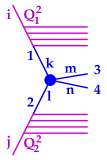
Figure 11: Parton-parton scattering, considering the Born process $1+2\to 3+4$. The solid lines represent partons (quarks, antiquarks, or gluons).

Starting from the differential parton-parton cross section Eq. (44), as shown in Appendix B Eq. (263), we may write

$$\frac{d^{3}\sigma_{\mathrm{hard}}^{ij}}{dx_{1}\,dx_{2}\,dt}\!=\!\!\sum_{K=1}^{12}\>\sum_{klmn\sim K}E_{\mathrm{QCD}}^{ik}(x_{1},Q_{1}^{2},\mu_{\mathrm{F}}^{2})E_{\mathrm{QCD}}^{jl}(x_{2},Q_{2}^{2},\mu_{\mathrm{F}}^{2})$$

$$\times\frac{\pi\alpha_{s}^{2}}{s^{2}}\left\{\frac{1}{g^{4}}\bar{\sum}|\mathcal{M}^{kl\to mn}|^{2}\right\}\frac{1}{1+\delta_{mn}}.$$ (107)

Compared to Eq. (263), we added a “$\sum_{K=1}^{12}$” term and the “$klmn\sim K$” condition to account for 12 different cross section classes, as discussed in section 3.3.5. The variables $x_{1}$ and $x_{2}$ are the momentum fractions of partons 1 and 2. This formula is very useful as a basis to generate the hard process in the parton ladder, in the Monte Carlo procedure, when employing the backward evolution.

However, we should not forget that we always need to distinguish four cases, namely both-sided, one-sided(lower), one-sided(upper), or no emissions. Correspondingly, we have four equations. For both-sided emissions, we use Eq. (107), with $\tilde{E}$ instead of $E$. In case of one-sided emission, we replace one of the $\tilde{E}_{\mathrm{QCD}}^{jl}$ by $\delta_{jl}\Delta^{j}$, and in case of no emissions, we replace both $\tilde{E}_{\mathrm{QCD}}^{jl}$ by $\delta_{jl}\Delta^{j}$.

3.4.1 Generating the hard process $\mathbf{1+2\to 3+4}$

We first have to know if we have both-sided, one-sided, or no emissions. So we first use the integrated cross sections $\sigma_{\mathrm{hard}}^{\mathrm{both\,}ij}$ , $\sigma_{\mathrm{hard}}^{\mathrm{upper\,}ij}$ , $\sigma_{\mathrm{hard}}^{\mathrm{lower\,}ij}\,$, and $\sigma_{\mathrm{hard}}^{\mathrm{none\,}ij}$ as weights to determine randomly what kind of emission we have.

In the case of both-sided emissions, we define, based on Eq. (107) with $\tilde{E}$ instead of $E$, the function $X_{klmn}^{ij}$ as

$$X_{klmn}^{ij}(z,t,x_{1})=\left\{\sigma_{\mathrm{hard}}^{\mathrm{both}\,ij}\right\}^{-1}$$ (108)

$$\;\times\tilde{E}_{\mathrm{QCD}}^{ik}(x_{1},Q_{1}^{2},\mu_{\mathrm{F}}^{2})\tilde{E}_{\mathrm{QCD}}^{jl}(x_{2},Q_{2}^{2},\mu_{\mathrm{F}}^{2})$$

$$\;\times\frac{\pi\alpha_{s}^{2}}{s^{2}}\left\{\frac{1}{g^{4}}\bar{\sum}|\mathcal{M}^{kl\to mn}|^{2}\right\}\frac{1}{1+\delta_{mn}},$$

with $z=x_{1}x_{2}$. We want to generate for given $i$ and $j$ the variables $z$, $t$ and $x_{1}$, according to the probability distribution

$$\mathrm{prob}(z,t,x_{1})=\sum_{K=1}^{12}\>\sum_{klmn\sim K}X_{klmn}^{ij}(z,t,x_{1}),$$ (109)

which is not trivial due to the fact that the expressions $X_{klmn}^{ij}$ contain singularities, as discussed in section 3.3.7, where we discussed the calculation of $\sigma_{\mathrm{hard}}^{\mathrm{both}\,ij}$ as a sum of integrals over $X_{klmn}^{ij}$. We also showed how to solve this problem. We had integrals of the form $\int X_{klmn}^{ij}dz\,dt\,dx_{1}$, which could be done after three coordinate transformations. Let us name the three integration variables $z_{1}$, $z_{2}$, and $z_{3}$, i.e.,

$$z_{1} =z=x_{1}x_{2}\,,$$ (110)

$$z_{2} =t\>,$$ (111)

$$z_{3} =x_{1}\,.$$ (112)

The three coordinate transformations $z_{i}\to u_{i}$ were defined as

$$\frac{\int_{a_{i}}^{z_{i}}g_{i}(x^{\prime})dx^{\prime}}{\int_{a_{i}}^{b_{i}}g_{i}(x^{\prime})dx^{\prime}}=\frac{u_{i}+1}{2},$$ (113)

for $i\in\{1,2,3\}$, with

$$g_{1}(z_{1}) \propto\qquad z_{1}^{-\delta_{\mathrm{hard}}-1},$$ (114)

$$g_{2}(z_{2}) \propto\qquad z_{2}^{-2},$$ (115)

$$g_{3}(z_{3}) \propto\left\{\begin{array}[]{cc}(1-z_{3})^{-1}&\mathrm{for}\,z_{3}>0.8\\ z_{3}\,^{-1}&\mathrm{for}\,z_{3}<0.8\end{array}\right..$$ (118)

There are two transformations for $z_{3}$, due to two singularities (at $0$ and $1$), which required a splitting of the integral. The three functions $g_{i}$ are useful also for the Monte Carlo generation of the variables $z_{i}$: One may first generate the $z_{i}$ according to $g_{i}$, by first generating uniform random numbers $u_{i}$ between -1 and 1, and then computing $z_{i}=z_{i}(u_{i})$ by inverting Eq. (113) (which is easy). Then, one accepts these proposals with the probability

$$p_{\mathrm{accept}}=\frac{\mathrm{prob}(z_{1},z_{2},z_{3})}{M\,g_{1}(z_{1})g_{2}(z_{2})g_{3}(z_{3})},$$ (119)

where $M$ has to be chosen such that $p_{\mathrm{accept}}\leq 1$. In this ratio, the singular parts of $\mathrm{prob}(z_{1},z_{2},z_{3})$ are canceled out by the $g_{i}$, and $p_{\mathrm{accept}}$ is therefore a smooth function of the variables, with an acceptable rate of rejections.

Then, for given $i$, $j$, $z_{1}$, $z_{2}$ and $z_{3}$, we generate $K$ and the flavors $k$ and $l$ according to

$$\mathrm{prob}(K,k,l)=\frac{\underset{klmn\sim K}{\underset{mn}{\sum}}X_{klmn}^{ij}(z_{1},z_{2},z_{3})}{\underset{K,k,l}{\sum}\underset{klmn\sim K}{\underset{mn}{\sum}}X_{klmn}^{ij}(z_{1},z_{2},z_{3})},$$ (120)

and for given $i$, $j$, $z_{1}$, $z_{2}$, $z_{3}$, $K$, $k$, and $l$, we generate $m$ and $n$ according to

$$prob(m,n)=\frac{X_{klmn}^{ij}(z_{1},z_{2},z_{3})|_{klmn\sim K}}{\underset{mn}{\sum}X_{klmn}^{ij}(z_{1},z_{2},z_{3})|_{klmn\sim K}}.$$ (121)

The two factors $\tilde{E}_{\mathrm{QCD}}^{ik}(...)$ and $\tilde{E}_{\mathrm{QCD}}^{jl}(...)$ do not depend on $m$ or $n$ and could be dropped but for the numerical procedures it is easier to keep them, since we may call the same functions as in the steps before.

In the case of one-sided emissions (on the upper side), we define

$$X_{kmn}^{ij}(x_{1},t)=\left\{\sigma_{\mathrm{hard}}^{\mathrm{upper}\,ij}\right\}^{-1}$$ (122)

$$\;\times\tilde{E}_{\mathrm{QCD}}^{ik}(x_{1},Q_{1}^{2},\mu_{\mathrm{F}}^{2})\Delta^{j}(Q_{2}^{2},\mu_{\mathrm{F}}^{2})$$

$$\;\times\frac{\pi\alpha_{s}^{2}}{s^{2}}\left\{\frac{1}{g^{4}}\bar{\sum}|\mathcal{M}^{kj\to mn}|^{2}\right\}\frac{1}{1+\delta_{mn}}.$$

We want to generate for given $i$ and $j$ the variables $x_{1}$ and $t$, according to the probability distribution

$$\mathrm{prob}(x_{1},t)=\sum_{K=1}^{12}\>\underset{kjmn\sim K}{\sum_{kmn}}X_{kmn}^{ij}(x_{1},t).$$ (123)

Again, we use the same coordinate transformations as already used for the integrations to compute $\sigma_{\mathrm{hard}}^{\mathrm{upper}\,ij}$. Here, with

$$z_{1} =x_{1},$$ (124)

$$z_{2} =t,$$ (125)

the transformations $z_{i}\to u_{i}$ were defined via Eq. (113) for $i\in\{1,2\}$, with

$$g_{1}(z_{1}) \propto\left\{\begin{array}[]{cc}(1-z_{1})^{-1}&\mathrm{for}\,z_{1}>0.8\\ z_{1}\,^{-1}&\mathrm{for}\,z_{1}<0.8\end{array}\right..$$ (128)

$$g_{2}(z_{2}) \propto\qquad z_{2}^{-2}.$$ (129)

We first generate the $z_{i}$ according to $g_{i}$ (first generating $u_{i}$, then inverting Eq. (113)) and then accept these proposals with the probability

$$p_{\mathrm{accept}}=\frac{\mathrm{prob}(z_{1},z_{2})}{M\,g_{1}(z_{1})g_{2}(z_{2})}.$$ (130)

Then for given $i$, $j$, $z_{1}$, and $z_{2}$, we generate $K$ and the flavor $k$ according to

$$\mathrm{prob}(K,k)=\frac{\underset{kjmn\sim K}{\underset{mn}{\sum}}X_{kmn}^{ij}(z_{1},z_{2})}{\underset{K,k}{\sum}\underset{kjmn\sim K}{\underset{mn}{\sum}}X_{kmn}^{ij}(z_{1},z_{2})},$$ (131)

and finally, for given $i$, $j$, $z_{1}$, $z_{2}$, $K$, and $k$, we generate $m$ and $n$ according to

$$\mathrm{prob}(m,n)=\frac{X_{kmn}^{ij}(z_{1},z_{2})|_{kjmn\sim K}}{\underset{mn}{\sum}X_{kmn}^{ij}(z_{1},z_{2})|_{kjmn\sim K}}.$$ (132)

In case of one-sided emissions on the lower side, we use the same algorithm as for the upper side, just exchanging the upper side and lower side variables and indices.

In case of no emissions, we define

$$X_{mn}^{ij}(t)=\left\{\sigma_{\mathrm{hard}}^{\mathrm{none}\,ij}\right\}^{-1}$$ (133)

$$\;\times\Delta^{i}(Q_{1}^{2},\mu_{\mathrm{F}}^{2})\Delta^{j}(Q_{2}^{2},\mu_{\mathrm{F}}^{2})$$

$$\;\times\frac{\pi\alpha_{s}^{2}}{s^{2}}\left\{\frac{1}{g^{4}}\bar{\sum}|\mathcal{M}^{ij\to mn}|^{2}\right\}\frac{1}{1+\delta_{mn}}.$$

We want to generate for given $i$ and $j$ the variable $t$, according to the probability distribution

$$\mathrm{prob}(t)=\sum_{K=1}^{12}\>\underset{ijmn\sim K}{\sum_{mn}}X_{mn}^{ij}(t),$$ (134)

which can be done by defining $z_{1}=t,$ and then defining the transformation $z_{1}\to u_{1}$ via Eq. (113) for $i=1$, with $g_{1}(z_{1})=z_{1}^{-2}$. We first generate $z_{1}$ according to $g_{1}$ (first generating $u_{1}$, then inverting Eq. (113)) and then accept these proposals with the probability

$$p_{\mathrm{accept}}=\frac{\mathrm{prob}(z_{1})}{M\,g_{1}(z_{1})}.$$ (135)

Then for given $i$, $j$, and $z_{1}$, we generate $K$ according to

$$\mathrm{prob}(K)=\frac{\underset{ijmn\sim K}{\underset{mn}{\sum}}X_{mn}^{ij}(z_{1})}{\underset{K}{\sum}\underset{ijmn\sim K}{\underset{mn}{\sum}}X_{mn}^{ij}(z_{1})},$$ (136)

and finally, for given $i$, $j$, $z_{1}$, and $K$, we generate $m$ and $n$ according to

$$\mathrm{prob}(m,n)=\frac{X_{mn}^{ij}(z_{1},z_{2})|_{ijmn\sim K}}{\underset{mn}{\sum}X_{mn}^{ij}(z_{1},z_{2})|_{ijmn\sim K}}.$$ (137)

3.4.2 Backward evolution

Knowing for given end flavours $i$ and $j$, the Born process variables $x_{1}$, $x_{2}$ and $t$, and the flavors $k$, $l$ (ingoing) and $m$, $n$ (outgoing), we generate the parton emission via backward evolution. The variable $t$ (Mandelstam variable) allows computing $p_{t}^{2}$ [see Eq. (85)], which corresponds in a unique fashion to some factorization scale $\mu_{\mathrm{F}}^{2}$, which is the starting value of the virtuality for the backward evolution. We therefore define $Q_{0}^{2}=\mu_{\mathrm{F}}^{2}$. Be $k$ the flavor of the corresponding parton.

In the following, we will use the symbol “$t$” as virtuality, to treat the parton evolution, it does not refer to the Mandelstam variable. We define $t_{0}=Q_{0}^{2}$.

We will in the following consider the evolution from $t_{1}$ to $t_{0}$ with $t_{1}<t_{0}$. We write the evolution equation [see Eq.(46)], using $\Delta^{k}(t_{1},t_{0})=\Delta^{k}(t_{0})/\Delta^{k}(t_{1})$, as

$$E_{\mathrm{QCD}}^{ik}\left(x,t_{1},t_{0}\right)=\frac{\Delta^{k}(t_{0})}{\Delta^{k}(t_{1})}\,\delta_{ik}\,\delta(1-x)$$ (138)

$$\qquad+\int_{t_{1}}^{t_{0}}\frac{dt}{t}\frac{\Delta^{k}(t_{0})}{\Delta^{k}(t)}\int\frac{dz}{z}\,\sum_{a}\bar{P}_{a}^{k}\!(t,z)\,E_{\mathrm{QCD}}^{ia}\left(\frac{x}{z},t_{1},t\right).$$

The integrand of the second term corresponds to a last branching in $[t,t+dt]$ , so the corresponding probability is

$$g(t)=\frac{1}{t}\,\frac{\Delta^{k}(t_{0})}{\Delta^{k}(t)}\int\frac{dz}{z}\sum_{a}\bar{P}_{a}^{k}(t,z)\frac{E_{\mathrm{QCD}}^{ia}(\frac{x}{z},t_{1},t)}{E_{\mathrm{QCD}}^{ik}(x,t_{1},t_{0})}.$$ (139)

Using Eq. (180), we get

$$g(t)=\frac{\partial}{\partial t}\left\{\frac{\Delta^{k}(t_{0})}{E_{\mathrm{QCD}}^{ik}(x,t_{1},t_{0})}\,\frac{E_{\mathrm{QCD}}^{ik}\left(x,t_{1},t\right)}{\Delta^{k}(t)}\right\}.$$ (140)

The probability of a last branching after some $t<t_{0}$ is $\int_{t}^{t_{0}}g(t^{\prime})dt^{\prime}$, which means that $t$ is generated via

$$\int_{t}^{t_{0}}g(t^{\prime})dt^{\prime}=r,$$ (141)

with $r$ being a uniform random number. The integral can be easily done, and we get

$$\int_{t}^{t_{0}}g(t^{\prime})dt^{\prime}=\left[\frac{\Delta^{k}(t_{0})\,E_{\mathrm{QCD}}^{ik}(x,t_{1},t^{\prime})}{\Delta^{k}(t^{\prime})\,E_{\mathrm{QCD}}^{ik}(x,t_{1},t_{0})}\right]_{t}^{t_{0}}=r,$$ (142)

which leads to

$$1-\frac{\Delta^{k}(t_{0})\,E_{\mathrm{QCD}}^{ik}(x,t_{1},t)}{\Delta^{k}(t)\,E_{\mathrm{QCD}}^{ik}(x,t_{1},t_{0})}=r,$$ (143)

Using $1-r$ instead of $r$, we obtain finally

$$R\equiv\frac{\Delta^{k}(t_{0})\,E_{\mathrm{QCD}}^{ik}(x,t_{1},t)}{\Delta^{k}(t)\,E_{\mathrm{QCD}}^{ik}(x,t_{1},t_{0})}=r,$$ (144)

for the generation of $t$ in the interval $[t_{1,}t_{0}]$.

So far we essentially followed the standard procedures, as explained in [2]. What makes things more difficult in the EPOS4 framework is the fact that we do evolutions for each of the parallel parton ladders, see Fig. 9, and there we consider the evolution starting from a parton, not from a proton. The initial condition for the evolution is

$$E_{\mathrm{QCD}}^{ik}\left(x,t_{\mathrm{ini}},t_{\mathrm{ini}}\right)=\delta(1-x)\delta_{ik},$$ (145)

and this singularity $\delta(1-x)$ needs some special attention. In Eq. (144), we need the full evolution function, which may be written as

$$E_{\mathrm{QCD}}^{ik}(x,t_{1},t)=\tilde{E}_{\mathrm{QCD}}^{ik}\left(x,t_{1},t\right)+\frac{\Delta^{k}(t)}{\Delta^{k}(t_{1})}\delta_{ik}\delta(1-x),$$ (146)

which separates the “smooth” and the “singular” part. For the generation of $t$ based on $R=r$, we consider the two cases $x=1$ and $x\neq 1$ separately.

For the case $x=1$, we have $R=1,$ which simply reflects the fact that there is no emission between $t_{1}$ and $t_{0}$, so we recover the initial condition $x=1$, and we are done for this case, the emission process is finished.

For the case $x\neq 1$, we have

$$R\equiv\frac{\Delta^{k}(t_{0})\,\tilde{E}_{\mathrm{QCD}}^{ik}(x,t_{1},t)}{\Delta^{k}(t)\,\tilde{E}_{\mathrm{QCD}}^{ik}(x,t_{1},t_{0})}=r,$$ (147)

which needs to be solved to get $t$. Some elementary root finder (like the bisection method) will do the job. Once this is done, for this value of $t$, the probability distribution for the momentum fraction $z$ of the last branching is obtained from Eq. (139) as

$$h(z)\propto\frac{1}{z}\sum_{a}\bar{P}_{a}^{k}(t,z)E_{\mathrm{QCD}}^{ia}(\frac{x}{z},t_{1},t),$$ (148)

which gives

$$h(z)\propto\frac{1}{z}\!\sum_{a}\bar{P}_{a}^{k}(t,z)\!\left\{\!\tilde{E}_{\mathrm{QCD}}^{ia}\!\left(\frac{x}{z},t_{1},t\right)\!+\!\frac{\Delta^{a}(t)}{\Delta^{a}(t_{1})}\delta_{ia}\delta(1-\frac{x}{z})\!\right\},$$ (149)

or

$$h(z)\propto\frac{1}{z}\!\sum_{a}\bar{P}_{a}^{k}(t,z)\tilde{E}_{\mathrm{QCD}}^{ia}\!\left(\frac{x}{z},t_{1},t\right)\!+\!\bar{P}_{i}^{k}(t,z)\frac{\Delta^{i}(t)}{\Delta^{i}(t_{1})}\delta(x-z),$$ (150)

for $z\geq x$. We need to distinguish again two cases, $z>x$ and $z=x$. The latter corresponds to a parton with a momentum fraction unity before the splitting (which is the initial value), so the emission process will be finished at the next iteration step. The probability for the $z=x$ case is

$$W_{1}=\frac{\bar{P}_{i}^{k}(t,x)\frac{\Delta^{i}(t)}{\Delta^{i}(t_{1})}}{\left\{\int_{x}^{1}\frac{dz}{z}\sum_{a}\bar{P}_{a}^{k}(t,z)\tilde{E}_{\mathrm{QCD}}^{ia}\left(\frac{x}{z},t_{1},t\right)\right\}+\bar{P}_{i}^{k}(t,x)\frac{\Delta^{i}(t)}{\Delta^{i}(t_{1})}},$$ (151)

where the integral can be done using the Gauss-Legendre method after an appropriate coordinate transform, splitting the integration domain into two parts, to treat separately the $z\to 0$ (for small $x$) and $z\to 1$ regions. This probability increases when (during the iteration) the virtuality approaches $t_{1}$ and the momentum fraction approaches unity. With the probability $W_{2}=1-W_{1}$, we have the case $z>x$, and here the probability distribution to generate $z$ is

$$h_{2}(z)\propto\frac{1}{z}\sum_{a}\bar{P}_{a}^{k}(t,z)\tilde{E}_{\mathrm{QCD}}^{ia}\left(\frac{x}{z},t_{1},t\right).$$ (152)

Finally, we generate the flavor $a$ according to

$$\bar{P}_{a}^{k}(t,z)\tilde{E}_{\mathrm{QCD}}^{ia}\left(\frac{x}{z},t_{1},t\right),$$ (153)

for the given values of $t$ and $z$ found earlier.

At each iteration step, we have these two cases, $z=x$ and $z>x$, where in one case the iteration is finished in the next step, with the initial value $x=1$, whereas in the other case, the iteration continues. So in any case, we eventually end up with the initial values.

3.4.3 Monte Carlo results versus cross section formulas for a single Pomeron

An elementary distribution (for tests) is the transverse momentum distribution $dn/dy\,dp_{t}$ for a given rapidity of primary partons, directly emitted in the Born process. Let us consider a single Pomeron, carrying the full energy, i.e., $x^{+}=x^{-}=1$, for an energy $E=\sqrt{s}=1\,$TeV, and let us consider $Q_{1}^{2}=Q_{2}^{2}=Q_{0}^{2}=O(1)$. We first investigate the “sea-sea” contribution. Combining Eq. (28) and Eq. (283), after integrating out the impact parameter $b$, we get (with a normalization constant $N$)

$$\frac{d^{2}n^{\mathrm{sea-sea}}}{dydp_{t}^{2}}=N\sum_{ij}\int\!dz^{+}dz^{-}$$ (154)

$$\quad E_{\mathrm{soft}}^{i}(Q_{0}^{2},z^{+})E_{\mathrm{soft}}^{j}(Q_{0}^{2},z^{-})\frac{d^{2}\sigma_{\mathrm{hard}}^{ij}}{dydp_{t}^{2}}(Q_{0}^{2},Q_{0}^{2},z^{+}z^{-}s),$$

with

$$\frac{d^{2}\sigma_{\mathrm{hard}}^{ij}}{dydp_{t}^{2}}(Q_{0}^{2},Q_{0}^{2},s_{\mathrm{lad}})$$ (155)

$$=\sum_{klmn}\int dx\,E_{\mathrm{QCD}}^{ik}(x_{1},Q_{0}^{2},\mu_{\mathrm{F}}^{2})E_{\mathrm{QCD}}^{jl}(x_{2},Q_{0}^{2},\mu_{\mathrm{F}}^{2})$$

$$\qquad\times\frac{\pi\alpha_{s}^{2}}{s^{2}}\left\{\begin{array}[]{c}\frac{1}{g^{4}}\end{array}\bar{\sum}|\mathcal{M}^{kl\to mn}|^{2}\right\}\frac{1}{1\!+\!\delta_{mn}}\,x_{1}x_{2}\frac{1}{x}$$ (157)

with $x_{1}=x+\begin{array}[]{c}\frac{p_{t}}{\sqrt{s_{\mathrm{lad}}}}\end{array}e^{y}$ and $x_{2}=\begin{array}[]{c}\frac{x_{1}}{x}\,\frac{p_{t}}{\sqrt{s_{\mathrm{lad}}}}\end{array}e^{-y}$. To compute $\mathcal{M}$, we need $s=x_{1}x_{2}s_{\mathrm{lad}}$ and $t=-p_{t}x_{1}\sqrt{s_{\mathrm{lad}}}e^{-y}$. In a similar way we get explicit formulas to compute the “val-val”, the “val-sea”, and the “sea-val” contribution. In Fig. 12,

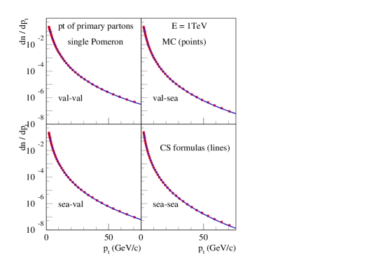
Figure 12: Transverse momentum distributions of primary partons for Pomerons of type “val-val”, “val-sea”, “sea-val”, and “sea-sea”. We compare the Monte Carlo results (points) to the corresponding curves obtained with the help of explicit cross section formulas (see text).

we show transverse momentum distributions (for $y=0$) of primary partons for Pomerons of type “val-val”, “val-sea”, “sea-val”, and “sea-sea”, based on these explicit formulas (lines), compared to the Monte Carlo results (points), using for the latter the methods explained in section 3.4.1. The Monte Carlo results agree with those based on cross section formulas. This may sound trivial, but in older EPOS versions with forward parton evolution, this was not the case. A great advantage of the new method is simply the fact that one can make rigorous tests, since the Monte Carlo uses the same “modules” as the cross section formulas ($E_{\mathrm{soft}}$, $E_{\mathrm{QCD}}$, and $\mathcal{M}$, all of them tabulated and available via interpolation). In both cases one uses evolution functions $E_{\mathrm{QCD}}$ representing all parton emissions, whereas in the old method the emissions in the Monte Carlo have been done one by one, and one needs to worry about additional elements like the reconstruction of the momentum four-vectors of the emitted partons.

3.4.4 EPOS PDFs

We may go one step further and provide formulas for inclusive momentum distributions for pp scattering with one single Pomeron (identical to the full multiple scattering results at high $p_{t}$, where factorization applies), again first considering “sea-sea”. Combining Eqs. (4,5,28,44), after integrating out the impact parameter $b$, we get

$$E_{3}E_{4}\frac{d^{6}\sigma^{\mathrm{sea-sea}}}{d^{3}p_{3}d^{3}p_{4}}$$ (158)

$$=\int dx^{+}dx^{-}V(1-x^{+})V(1-x^{-})\sum_{ij}\int\!dz^{+}dz^{-}$$

$$\quad F_{\mathrm{sea\,1}}(x^{+},0)\,F_{\mathrm{sea}\,2}(x^{-},0)\,E_{\mathrm{soft}}^{i}(Q_{0}^{2},z^{+})E_{\mathrm{soft}}^{j}(Q_{0}^{2},z^{-})$$

$$\quad\sum_{klmn}\int\!\int\!\!dx_{1}dx_{2}E_{\mathrm{QCD}}^{ik}(x_{1},Q_{0}^{2},\mu_{\mathrm{F}}^{2})E_{\mathrm{QCD}}^{jl}(x_{2},Q_{0}^{2},\mu_{\mathrm{F}}^{2})$$

$$\quad\frac{1}{32s\pi^{2}}\bar{\sum}|\mathcal{M}^{kl\to mn}|^{2}\delta^{4}(p_{1}+p_{2}-p_{3}-p_{4})\frac{1}{1+\delta_{mn}},$$

with $s=\xi^{+}\xi^{-}s_{\mathrm{pp}}$ being the squared energy of the Born process, with $\xi_{1}=x^{+}z^{+}x_{1}$ and $\xi_{2}=x^{-}z^{-}x_{2}$. For “val-val”, combining Eqs. (4,5,18,44), we get

$$E_{3}E_{4}\frac{d^{6}\sigma^{\mathrm{val-val}}}{d^{3}p_{3}d^{3}p_{4}}$$ (159)

$$=\int dx^{+}dx^{-}V(1-x^{+})V(1-x^{-})\sum_{ij}\int\!dz^{+}dz^{-}$$

$$\quad F_{\mathrm{val}\,1}^{i}(z^{+},x^{+}-z^{+},0)\,F_{\mathrm{val}\,2}^{j}(z^{-},x^{-}-z^{-},0)$$

$$\quad\sum_{klmn}\int\!\int\!\!dx_{1}dx_{2}E_{\mathrm{QCD}}^{ik}(x_{1},Q_{0}^{2},\mu_{\mathrm{F}}^{2})E_{\mathrm{QCD}}^{jl}(x_{2},Q_{0}^{2},\mu_{\mathrm{F}}^{2})$$

$$\quad\frac{1}{32s\pi^{2}}\bar{\sum}|\mathcal{M}^{kl\to mn}|^{2}\delta^{4}(p_{1}+p_{2}-p_{3}-p_{4})\frac{1}{1+\delta_{mn}},$$

with $s=\xi^{+}\xi^{-}s_{\mathrm{pp}}$ being the squared energy of the Born process, with $\xi_{1}=z^{+}x_{1}$ and $\xi_{2}=z^{-}x_{2}$. Corresponding formulas can be found for the “val-sea”, and the “sea-val” contribution (we do not consider “psoft” here, since it only contribute at low $p_{t}$). As a consequence, the complete momentum distribution (the sum of the four contributions) may be written as

$$E_{3}E_{4}\frac{d^{6}\sigma}{d^{3}p_{3}d^{3}p_{4}}$$ (160)

$$=\sum_{klmn}\int\!\!\int\!\!d\xi_{1}d\xi_{2}\,f_{\mathrm{PDF}}^{k}(\xi_{1},\mu_{\mathrm{F}}^{2})f_{\mathrm{PDF}}^{l}(\xi_{2},\mu_{\mathrm{F}}^{2})$$

$$\quad\frac{1}{32s\pi^{2}}\bar{\sum}|\mathcal{M}^{kl\to mn}|^{2}\delta^{4}(p_{1}+p_{2}-p_{3}-p_{4})\frac{1}{1+\delta_{mn}},$$

with

$$f_{\mathrm{PDF}}^{k}(\xi,\mu_{\mathrm{F}}^{2})$$

$$=\int dx\,dz\,dy\Big{\{}\sum_{i}V(1-x)\,F_{\mathrm{sea}}(x,0)\,E_{\mathrm{soft}}^{i}(Q_{0}^{2},z)$$

$$\qquad\qquad\qquad E_{\mathrm{QCD}}^{ik}(y,Q_{0}^{2},\mu_{\mathrm{F}}^{2})\delta(\xi-xzy)\Big{\}}$$ (161)

$$\quad+\int dx\,dz\,dy\Big{\{}\sum_{i}V(1-x)F_{\mathrm{val}}^{i}(z,x-z,0)$$

$$\qquad\qquad\qquad E_{\mathrm{QCD}}^{ik}(y,Q_{0}^{2},\mu_{\mathrm{F}}^{2})\delta(\xi-zy)\Big{\}}.$$

These are the “EPOS4 PDFs” (parton distribution functions), composed of a “sea” contribution (the first integral) and a “valence” contribution (the second integral).

Eq. (160) is identical to the “usual” factorization formula, which everybody uses. However, in our case, it represents the single Pomeron case. The full simulation, i.e., the full multiple scattering case, provides the same result, but only at large transverse momenta, as we will show later.

To make it very clear: In the EPOS4 formalism, we cannot use PDFs as an input, we need several “modules” such as vertex functions ($V$, $F_{\mathrm{sea}}$, $F_{\mathrm{val}}^{i}$) and evolution functions ($E_{\mathrm{soft}}^{i}$, $E_{\mathrm{QCD}}^{ik}$) to construct the “building blocks” $G_{QCD}$, and then $G$ (cut single Pomeron), being the basis of our multiple scattering scheme. But we can use these “modules” to construct EPOS4 PDFs.

Let us first compare the EPOS4 PDFs with other choices and with data. At least the quark parton distribution functions can be tested and compared with experimental data from deep inelastic electron-proton scattering. The leading order structure function $F_{2}$ is given as

$$F_{2}=\sum_{k}e_{k}^{2}\,x\,f_{\mathrm{PDF}}^{k}(x,Q^{2}),$$ (162)

$$\mathrm{with}\qquad x=x_{B}=Q^{2}/(2p\cdot q),$$ (163)

$$Q^{2}=-q^{2},$$ (164)

where $p$ is the momentum of the proton and $q$ the momentum of the exchanged photon. In Fig. 13,

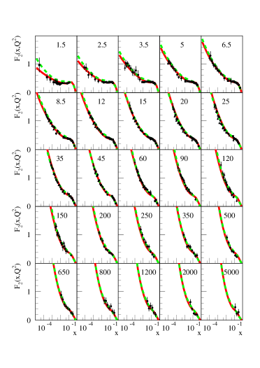
Figure 13: $F_{2}$ as a function of $x$ for different values of $Q^{2}$, the latter one indicated (in units of $\mathrm{GeV}^{2}$) in the upper right corners of each sub-plot . The red curves refer to EPOS PDFs, the green ones to CTEQ PDFs, and the black points are data from ZEUS and H1.

we plot $F_{2}$ as a function of $x$ for different values of $Q^{2}$, the latter one indicated (in units of $\mathrm{GeV}^{2}$) in the upper right corners of each sub-plot . The red curve refers to EPOS PDFs, the green one to CTEQ PDFs [17], and the black points are data from ZEUS [18] and H1 [19, 20, 21]. The two PDFs give very similar results, and both are close to the experimental data.

Having checked the EPOS PDFs, we will use these functions to compute the jet (parton) cross section for pp at 13 TeV, using Eq. (160), integrating out the momentum of the second parton and the azimuthal angle of the first parton, which finally gives (see Eq. (283), with $E_{\mathrm{QCD}}^{ik}$ replaced by $f_{\mathrm{PDF}}^{k}$, and $s_{\mathrm{lad}}$ by $s_{\mathrm{pp}}$)

$$\frac{d^{2}\sigma}{dy\,dp_{t}^{2}}=\sum_{klmn}\int dx\,f_{\mathrm{PDF}}^{k}(x_{1},\mu_{\mathrm{F}}^{2})f_{\mathrm{PDF}}^{l}(x_{2},\mu_{\mathrm{F}}^{2})$$

$$\qquad\times\frac{\pi\alpha_{s}^{2}}{s^{2}}\left\{\begin{array}[]{c}\frac{1}{g^{4}}\end{array}\bar{\sum}|\mathcal{M}^{kl\to mn}(s,t)|^{2}\right\}\frac{1}{1\!+\!\delta_{mn}}\,x_{1}x_{2}\frac{1}{x}\,,$$ (166)

$$\mathrm{\quad with}\;x_{1}=x+\begin{array}[]{c}\frac{p_{t}}{\sqrt{s_{\mathrm{pp}}}}\end{array}e^{y},\,x_{2}=\begin{array}[]{c}\frac{x_{1}}{x}\,\frac{p_{t}}{\sqrt{s_{\mathrm{pp}}}}\end{array}e^{-y},$$ (169)

$$\qquad\qquad s=x_{1}x_{2}\sqrt{s_{\mathrm{pp}}},\,t=-p_{t}x_{1}\sqrt{s_{\mathrm{pp}}}e^{-y},$$ (170)

with $\left\{...\right\}$being the form the squared matrix elements are usually tabulated, with $\alpha_{s}=g^{2}/4\pi$. We define the parton yield $dn/dp_{t}dy$ as the cross section $d\sigma/dy\,dp_{t}^{2}$, divided by the inelastic pp cross section, times $2\,p_{t}$, showing the result in Fig. 14.

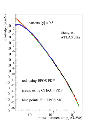
Figure 14: Parton yield $dn/dp_{t}dy$ for pp at 13 TeV. We show results based on EPOS PDFs (red full line), CTEQ PDFs (green dashed line), the full EPOS simulation (blue circles), and experimental data from ATLAS (black triangles).

We show results based on EPOS PDFs (red full line), CTEQ PDFs [17] (green dashed line), the full EPOS simulation (blue circles), and experimental data from ATLAS [22] (black triangles). At large values of $p_{t}$, all the different distribution agree, whereas at low $p_{t}$ the EPOS Monte Carlo simulation results (using the full multiple scattering scenario) are significantly below the PDF results, as expected due to screening effects.

Let us consider the production of charmed primary partons ($c$ and $\bar{c}$) for pp at 13 TeV, still based on EPOS4 PDFs, according to Eq. (166). The term “primary” means that here we do not consider charm created in the timelike cascade (in the full simulation we do, of course). We have the elementary Born scattering $kl\to mn$, where $k,l$ are the incoming and $m,n$ the outgoing parton flavors. Let us note light flavor partons as “$L$” and heavy flavor ones (here charm) as “$H$”. We may produce charm via $HL\to HL$ (“flavor excitation”) or via $LL\to H\bar{H}$. We will in the following consider two cases: including flavor excitation (incl FlavEx) or not (w/o FlavEx), for two calculations: based on EPOS4 PDFs and based on CTEQ PDFs [17], see Fig. 15.

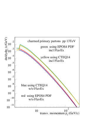
Figure 15: Transverse momentum distribution of charm quarks ($c$ and $\bar{c}$), based on EPOS PDFs and CTEQ PDFs. In both cases, we show results including flavor excitation (incl FlavEx) or not (w/o FlavEx). The “jumps” mark the activation of charm flavor excitation for $\mu_{\mathrm{F}}>2\,m_{c}$.

The EPOS4 results are shown as green (incl FlavEx) and red lines (w/o FlavEx), the CTEQ based results are shown as yellow (incl FlavEx) and blue lines (w/o FlavEx). The EPOS4 and the CTEQ results are similar, at large $p_{t}$ they are even identical. In both cases, the flavor excitation contribution is largely dominant, over the whole $p_{t}$ range, above some threshold. In Fig. 16,

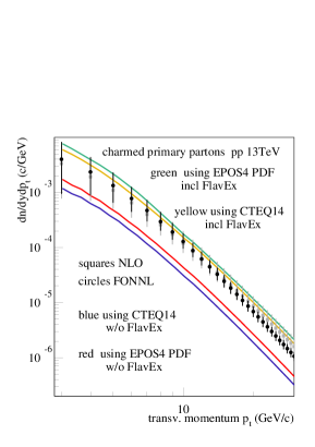
Figure 16: Transverse momentum distribution of charm quarks ($c$ and $\bar{c}$), based on EPOS PDFs and CTEQ PDFs. In both cases, we show results including flavor excitation (incl FlavEx) or not (w/o FlavEx). The black circles represent FONLL results, and the gray squares NLO calculations.

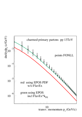
Figure 17: Transverse momentum distribution of charm quarks ($c$ and $\bar{c}$), based on EPOS PDFs including flavor excitation fully (incl FlavEx) or with a reduction factor $k_{\mathrm{FE}}$ (FlavEx*$k_{\mathrm{FE}}$). The black circles represent FONLL results.

we plot the same four curves (EPOS4 and the CTEQ based, with and without flavor excitation), in a reduced $p_{t}$ range, together with FONLL and NLO calculations [23], the latter represented by black circles (FONLL) and gray squares (NLO). The NLO results (at least at large $p_{t})$ are quite close to the ones based on EPOS4 and CTEQ PDFs. In the EPOS4 framework, we use a k-factor equal unity; however, we use a “variable flavor number scheme”, i.e., the number of allowed flavors depends on the virtuality, which means at large $p_{t},$ which is correlated with large virtualities, we easily produce heavy flavor. Concerning the FONLL results, they drop with increasing $p_{t}$ considerably below the EPOS4 and the CTEQ based results. In order to be close to FONLL, we multiply the flavor excitation contribution by a factor $k_{\mathrm{FE}}<1,$ the result for a numerical value of 0.4 is shown in Fig. 17.

3.4.5 The pseudosoft contribution

In the previous examples, only the contributions “sea-sea”, “val-val”, “sea-val”, and “val-sea” were considered. The PDFs are actually a sum of “sea” and “val”. There is, however, also a “pseudosoft” contribution, see Eq. (43). We expect the “pseudosoft” Pomeron to have an internal structure, allowing hard processes. We assume some probability distribution $P(X)$ with $\left\langle X\right\rangle=O(1)$ of $X=Q^{2}/Q_{\mathrm{sat}}^{2}$, with $Q^{2}$ being the scale associated with the hard process, and then for given $Q^{2}$, a probability distribution of the form

$$E_{\mathrm{psoft}}^{i}(Q^{2},z^{+})E_{\mathrm{psoft}}^{j}(Q^{2},z^{-})\,\frac{1}{16\pi s^{2}}\bar{\sum}|\mathcal{M}^{ij\to mn}|^{2}\begin{array}[]{c}\frac{1}{1+\delta_{mn}}\end{array}$$ (171)

to generate a particular hard process. We expect the production of partons with transverse momenta of the order of $Q_{\mathrm{sat}}^{2}$, in the range 1-10 GeV/c.

3.4.6 A result for full EPOS

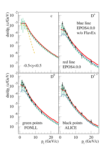
Figure 18: Charmed partons and hadrons in pp collisions at 7 TeV. We show EPOS4 simulations, compared to FONLL results and ALICE data.

In the examples discussed in 3.4.4, based on EPOS PDFs, only primary partons were considered (directly produced in the Born process). To get the complete picture (but without considering secondary interactions as hydro evolution and hadronic rescattering), we employ the full EPOS4 approach for primary scatterings, including multiple scattering, and also including the timelike cascade, which includes Born processes like $g+g\to g+g$, where each of the outgoing gluons may split into a $c\bar{c}$ pair. In Fig. 18 (upper left panel), we show the corresponding transverse momentum distribution of charmed quarks (including antiquarks) in pp scattering at 7 TeV, compared to FONLL results [23]. The yellow dashed line represents the “pseudosoft” contribution, which visibly contributes at low transverse momentum, as expected.

In the full (primary scattering) approach, we consider not only the full partonic evolution (initial-state and final-state cascade) but also hadronization. This will be discussed in detail in section 4, but let us anticipate here some basic features: cut parton ladders correspond in general to two chains of partons $q-g-...-g-\bar{q}$ identified as kinky strings, with $q$ referring to light flavor partons, and $g$ to gluons. The Born process or branchings in the spacelike or the timelike cascade may lead to $Q\bar{Q}$ production, where $Q$ refers to “heavy flavor” (HF) quarks, i.e., charm or bottom. In this case, we end up with parton chains of the type $q-g-...-g-\bar{Q}$ and $Q-g-...-g-q$, which will decay (among others) into HF hadrons. In Fig. 18, we show transverse momentum spectra of $D^{+}$, $D^{-}$ mesons (upper right), $D^{0}$ mesons (lower left), and $D^{+*}$, $D^{-*}$ mesons (lower right) in pp collisions at 7 TeV. The red lines refer to EPOS4 simulations, the green points to FONLL calculations [23], and the black points to ALICE data [24]. We also show as blue lines the EPOS4 results without flavor excitation. Many more results can be found in [6].

4 From partons to strings: color flow

In the previous section, we were discussing in detail the partonic structure of the EPOS4 building blocks, the Pomerons. This allows us to compute the weights of multiple Pomeron configurations and generate these. In the present section, we will discuss how to transform these partonic structures into strings. The strings are then the basis of hadron production via string decay or of the formation of a “core” (in case of high densities), serving as an initial condition of a hydrodynamical evolution. The formation of strings for a particular partonic configuration is based on the associated color flow.

4.1 An example

In order to be as general as possible, let us consider a collision of two nuclei, as shown in Fig. 19, where we consider the partonic configuration of two colliding nuclei $A$ and $B$, each one composed of two nucleons. Dark blue lines mark active quarks, red dashed lines active antiquarks, and light blue thick lines projectile and target remnants (nucleons minus the active (anti)quarks). We have two scatterings of “sea-sea” type, and one of “val-sea” type. We consider each incident nucleon as a reservoir of three valence quarks plus quark-antiquark pairs. The “objects” which represent the “external legs” of the individual scatterings are colorwise “white”: quark-antiquark pairs in most cases as shown in the figure, but one may as well have quark-diquark pairs or even antiquark-antidiquark pairs – in any case, a $3$ and a $\bar{3}$ color representation.

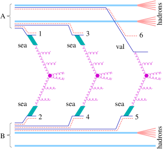
Figure 19: Partonic configuration of two colliding nuclei $A$ and $B$, each one composed of two nucleons, with three scatterings (from three cut Pomerons). Dark blue lines mark active quarks, red dashed lines active antiquarks, and light blue thick lines projectile and target remnants. One of the target nucleons is just a spectator.

Let us for simplicity consider the quark-antiquark option, and first of all look at the “sea” cases (on the projectile or the target side). In each case, a quark-antiquark pair is emitted as final-state timelike (TL) parton pair (marked 1,2,3,4,5) and a spacelike (SL) “soft Pomeron” (indicated by a thick cyan line), which is meant to be similar to the QCD evolution, but emitting only soft gluons, which we do not treat explicitly. Then emerging from this soft Pomeron, we see a first perturbative SL gluon (another possibility is the emission of a quark, to be discussed later), which initiates the partonic cascade. In the case of “val”, we also have a quark-antiquark pair as external leg, but here first an antiquark is emitted as TL final particle (marked 6), plus an SL quark starting the partonic cascade.

In the case of multiple scattering as in Fig. 19, the projectile and target remnants remain colorwise white, but they may change their flavor content during the multiple collision process. The quark-antiquark pair “taken out” for a collision (the “external legs” for the individual collisions), may be $u-\bar{s}$, then the remnant for an incident proton has flavor $uds$. In addition, the remnants get massive, much more than simply resonance excitation. We may have remnants with masses of $10\,\mathrm{GeV/c^{2}}$ or more, which contribute significantly to particle production (at large rapidities).

In the following, we discuss the color flow for a given configuration, as for example the one in Fig. 19. Since the remnants are by construction white, we do not need to worry about them, we just consider the rest of the diagram. In addition, colorwise, the “soft Pomeron” part behaves as a gluon. Finally, we use the following convention for the SL partons which are immediately emitted: We use for the quarks an array away from the vertex, and for the antiquarks an array towards the vertex. The diagram equivalent to Fig. 19 is then the one shown in Fig. 20.

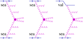
Figure 20: Configuration colorwise equivalent to the one of Fig. 19. The outgoing antiquarks are drawn as incoming quarks (arrows towards vertices).

Based on Fig. 20, considering the fact that in the parton evolution and the Born process, the gluons are emitted randomly to the right or to the left, we show in Fig. 21

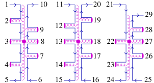
Figure 21: A possible color flow diagram for the three scatterings of Fig. 20.

a possible color flow diagram for the three scatterings. Horizontal lines refer to TL partons, which later undergo a timelike cascade, while the vertical lines refer to spacelike intermediate partons. We added integers just to mark the different TL partons. For the leftmost scattering, starting from one “end”, say “1”, we follow the color flow to “5”, and then starting from “6” to “10”, so we get two chains: 1-2-3-4-5 and 6-7-8-9-10. The end partons of each chain are always quarks or antiquarks, and the inner partons are gluons. Similar chains are obtained for the second scattering, 11-12-13-14-15 and 16-17-18-19-20, and for the third scattering, 21-22-23-24 and 25-26-27-28-29. These chains of partons will be mapped (in a unique fashion) to kinky strings, where each parton corresponds to a kink, and the parton four-momentum defines the kink properties, as already done in earlier EPOS versions [11]. In the following, we simplify our graphs, instead of Fig. 21 we use a diagram as shown in Fig. 22,

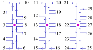
Figure 22: Simplified color flow diagram for the three scatterings of Fig. 21. The dot indicates the Born process.

where we do not plot the gluon lines explicitly, since the double lines with arrows in opposite direction allow us perfectly to identify the gluons.

Considering these examples, it is useful to define “initial partons”, being those which are immediately emitted as TL partons before the parton evolution starts. In the case of the type “sea”, a quark and an antiquark (or diquark) are emitted, in Fig. 21 the partons 1,10 and 5,6 and 11,20 and 15,16 and 24,25. The partons like 2,3,4 or 7,8,9 are emitted either in the spacelike partonic cascade (like 2,4,7,9) or in the Born process (3,8). In case of “val”, a TL antiquark is emitted, namely the antiquark 21. Here, an SL quark enters the partonic cascade (vertical line). Parton 29 is not an initial parton, it is the first parton emitted in the SL cascade.

The above discussion demonstrates for an example, how to obtain “chains of partons” (and then kinky strings), based on an analysis of the color flow. But the picture is not yet complete. In general, each emitted parton initiates a timelike cascade, as shown in Fig. 23,

(a)                   (b)                
      

Figure 23: timelike cascade, with Feynman diagram (a) and the corresponding color flow diagram (b).

and this has to be taken into account when constructing the “chains of partons” based on color flow. In the following, we discuss the general rules, applicable for any multiple scattering configuration, in pp or AA, including timelike cascades.

4.2 The initial TL partons and the initial SL partons

Even in the case of multiple scatterings, the projectile and target remnants remain color white and fragment independently, and correspondingly the external legs of the individual scatterings are white. They are quark-antiquark pairs (or less likely quark-diquark pairs). These external legs emit immediately TL partons, referred to as “initial partons”, as compared to the partons emitted later during the parton evolution. The number and the properties of the initial partons for each individual scattering depend on the Pomeron type.

We have four scattering (or Pomeron) types: “sea-sea”, “val-sea”, “sea-val”, and “val-val”, where the first concerns the projectile, the second the target. In the case of “sea” (on the projectile or the target side), we have three cases: “sea($g$)” and “sea($q$)”, and “sea($\bar{q}$)”. The notion of “sea” always means that there is first a “soft pre-evolution”. In case of “sea($g$)” the first parton entering the spacelike (SL) cascade, is a gluon, in case of “sea($q$)” a quark, and in case of “sea($\bar{q}$)” an antiquark. These partons are referred to as “initial SL partons”. In Fig. 24,

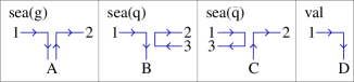
Figure 24: Initial TL partons 1,2,3, for the cases “sea($g$)” and “sea($q$)”, “sea($\bar{q}$)”, and “val”, on the projectile side. The “initial SL partons” which initiate the SL cascade are marked A, B, C, D.

we show the four possibilities, for the projectile side. In case of “sea($g$)”, the “external leg” is a quark-antiquark pair, which emits a TL quark and a TL antiquark (2 and 1 in Fig. 24) and an SL gluon, which starts the SL cascade and is color connected to 1 and 2. In the case of sea($q$), in addition to 1 and 2, the TL antiquark 3 is emitted, and an SL quark is initiating the cascade, color connected to 1. The TL antiquark 3 is color connected to the TL quark 2 (so 2 and 3 constitute a “little” string, which will be given a small amount of energy). In case of sea($\bar{q}$), in addition to 1 and 2, a TL quark is emitted (3), color connected to the TL antiquark 1. Here an SL antiquark is initiating the SL cascade, color connected to 2. Finally, in the case of val, a TL antiquark is emitted (1), and we have an SL quark initiating the SL cascade, color connected to antiquark 1. The discussion for the target side is identical, we just use a somewhat different graphical representation, as shown in Fig. 25.

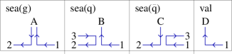
Figure 25: Initial TL partons 1,2,3, for the cases “sea($g$)” and “sea($q$)”, “sea($\bar{q}$)”, and “val”, on the target side. The “initial SL partons” which initiate the SL cascade are marked A, B, C, D.

Here the arrows from 1 (emitted antiquark) to 2 (emitted quark) go from right to left.

Knowing the color connections of the initial partons among each other and with respect to the SL partons initiating the SL cascade, we need as a next step to extend the construction of the color connections to the SL cascade.

4.3 The spacelike (SL) parton evolution

Whereas for technical reasons, we employ (for each individual scattering) a backward evolution method to generate the kinematical variables of the partons, we will here consider the SL parton evolution starting from the “initial SL partons” towards the Born process. To have a unique definition of the color flow in the direction of the evolution, we define (instead of “right” and “left”) the terms “color side” and “anticolor side”, as shown in Fig. 26.

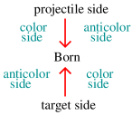
Figure 26: Defining color and anticolor side for the SL evolution. The red arrows represent the directions of the evolutions, starting from the projectile or the target side.

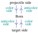
Figure 27: The color arrows for a gluon evolution, from the projectile or the target side towards the Born process.

In this way, in the direction of the evolution, “color side” corresponds to “right”, and “anticolor side” to “left”. For the evolution of an SL gluon, the two arrows representing the color flow are always such that the forward arrow (in the direction of the evolution) is on the “color side”, and the backward arrow on the “anticolor side”, as shown in Fig. 27.

The aim is to construct the color flow, i.e., sequences of TL partons $j_{1}-j_{2}-...-j_{n}$ (like the sequence $1-2-3-4-5$ shown in in Fig. 22). To do so we number all the timelike partons $j=1,2,3...$ (starting with the initial ones). Referring to this parton numbering $j$, we define an integer array, the connection array $n_{\mathrm{CJ}}^{\eta}(i,j)$ for TL partons $j$, defined such that

$$j_{\mathrm{before}}=n_{\mathrm{CJ}}^{\eta}(1,j)$$ (172)

defines the TL parton in the chain just before and

$$j_{\mathrm{after}}=n_{\mathrm{CJ}}^{\eta}(2,j)$$ (173)

the TL parton just after the parton $j$. So for the example of the chain $1-2-3-4-5$ shown in in Fig. 22, considering the subsequence $2-3-4$, for $j=3$, we have $j_{\mathrm{before}}=n_{\mathrm{CJ}}^{\eta}(1,j)=2$ and $j_{\mathrm{after}}=n_{\mathrm{CJ}}^{\eta}(2,j)=4$. When we talk about sequences $j_{1}-j_{2}-...-j_{n}$, we have two options (which we use both): following the color flow ($\to$) or the anticolor flow ($\leftarrow$). In the first case, we use $\eta=1$, in the second one $\eta=2$. The index $\eta$ is referred to as “color orientation”. At the end of the emission procedures, this array will contain the complete information about which partons are color connected.

For the evolution process, it is useful to define the “current SL parton” (say parton $a$), based on which the emission process is considered ($a\to b+c$), with an SL parton $b$ and a TL $c$. In the next step, parton $b$ is considered to be the current SL parton, and so on. During the evolution procedure, we use for the current SL parton some integer array, the connection array $n_{\mathrm{CC}}(i,k)$ for the current SL parton, providing information to which TL partons the current SL parton is connected to. Here,

$$j_{\mathrm{proj}}=n_{\mathrm{CC}}(i,1)$$ (174)

refers to the connection on the projectile side and

$$j_{\mathrm{targ}}=n_{\mathrm{CC}}(i,2)$$ (175)

to the connection on the target side. For gluons, the index $i=1$ refers to the color side, and $i=2$ to the anticolor side. In the case of quarks and antiquarks, only $i=1$ will be used, and the value for $i=2$ is zero.

Consider for example the first SL parton on the projectile side, as shown in Fig. 28.

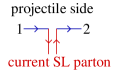
Figure 28: gluon as first SL parton, connected to 1 (color side) and 2 (anticolor side).

The first “current parton” is a gluon. It is color connected to 1 (color side) and 2 (anticolor side), so we have $n_{\mathrm{CC}}(1,k)=1$ and $n_{\mathrm{CC}}(2,k)=2$, here for $k=1$, since we consider the projectile side.

In the next step, let us assume we have a gluon emission (parton $3$). Concerning color flow, we have two possibilities, an emission on the color side or the anticolor side, as shown in Fig. 29.

(a)                                   (b)                                                                                         
         

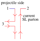
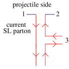
Figure 29: The two possibilities of color flow for a gluon emission: (a) emission on the color side, corresponding to $\eta=1$ or (b) the anticolor side, corresponding to $\eta=2$.

In the first case, we have a “subchain” $1\to 3$, i.e., for the new TL parton $j=3$, we have $n_{\mathrm{CJ}}^{\eta}(1,j)=1$, and since we follow the color flow ($\to$), we use $\eta=1$. In the second case, we have a “subchain” $2\to 3$, i.e., for the new TL parton $j=3$, we have $n_{\mathrm{CJ}}^{\eta}(1,j)=2$, and since we follow the anticolor flow ($\to$), we use $\eta=2$. In other words, the two choices correspond to the two choices $\eta=1$ and $\eta=2$, and they are chosen randomly.

Having discussed the case of a gluon being the first emitted TL parton (marked 3), let us discuss the case of the first emitted TL parton being a quark (also marked 3). Here, we have no choice, as can be seen in Fig. 30.

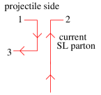
Figure 30: The two possibilities of color flow for the first emission. The l.h.s. of the figure corresponds to the color orientation $\eta=1$, the r.h.s. to $\eta=2$

Here, we have mandatory color orientation $\eta=1$, the quark is emitted on the color side. And in the case of antiquark emission, we have $\eta=2$. The color orientation determines which of the partons, $n_{CC}(1,k)$ or $n_{CC}(2,k)$, is the one the new emitted TL parton is connected to. In the first case (quark emission), we have for the new parton $j=3$ the connection $n_{\mathrm{CJ}}^{\eta}(1,j)=n_{\mathrm{CC}}(\eta,k)=1$ (using $\eta=1$). In the second case (antiquark emission), we have for the new parton $j=3$ the connection $n_{\mathrm{CJ}}^{\eta}(1,j)=n_{\mathrm{\mathrm{CC}}}(\eta,k)=2$ (using $\eta=2$) always for $k=1$ (projectile).

So far we treated the first TL emission of the SL parton cascade, and we explained how to use the two arrays $n_{\mathrm{CJ}}$ and $n_{\mathrm{\mathrm{CC}}}$. In a similar way we can treat all subsequent emissions. However, an emitted TL parton will, in general, develop a TL parton cascade, and we first need to deal with that. We will discuss this in the next section.

4.4 The timelike cascade

Here we consider the situation, at some stage of the SL cascade, where starting from some “current SL parton” we have an emitted TL parton with (some unique) number $j$, and suppose we know the color orientation $\eta$ of this TL emission and the color connection array $n_{\mathrm{CJ}}^{\eta}(1,j)$. To simplify the notation (reduce the indices), we define for given $\eta$ and given $j$ the integer $n_{\mathrm{CR}}(1)=n_{\mathrm{CJ}}^{\eta}(1,j)$. There is also the variable $n_{\mathrm{CR}}(2)$, referring to the connected parton on the other side, not yet known here, but important in case of TL emissions in the Born process, to be discussed later.

We need to reconstruct the color flow of the TL cascade and connect it to the rest of the diagram, knowing the connected parton $n_{\mathrm{CR}}(1)$, which points to the previous TL parton in the color flow chain, and the color orientation $\eta$. We assume that we know at this stage the complete TL cascade, with the flavors and four-momenta of all the partons. Let us consider a concrete case as shown in Fig. 31,

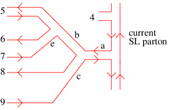
Figure 31: Color flow in TL cascade.

with $\eta=1$ (emission of a gluon on the color side), and with the previous TL parton in the color flow chain being $n_{\mathrm{CR}}(1)=4$ (assuming that the indices 1,2,3 have been used already before). We also assume here that parton 4 is a final particle. We actually use a rigorous unique numbering (1,2,3,…) only for the final partons, for the intermediate partons in the plot we use symbols $a,\,b,\,c\ldots$. The first emitted TL parton $a$ splits into $b$ and $c$, and these daughter partons split again in partons, and at the end, we have final partons 5, 6, 7, 8, 9. At this stage (after realizing the TL cascade, as discussed earlier), the planar structure is already fixed, and each vertex like $a\to b+c$ has a clearly defined “first daughter” D1 (upper) and a “second daughter“ D2 (lower), when considering the evolution from right to left. The fact that there is some freedom concerning the exchange of D1 and D2 is taken care of during the evolution. Here, we simply need to identify the final partons, associate a number (the next free integer), and reconstruct the color connections. This may be done as follows:

1. Define the initial parton to be the current parton.

2. Starting from the current parton, loop over all the first daughters until a final parton is reached, now being the new current parton.

3. Update connection information for the current parton itself, its parent, and the second daughter.

4. If the second daughter is not final, consider it to be the current parton, go back to 2,

5. If the second daughter is final, define the parent to be the current parton, go back to 3.

In this way, we move through the whole diagram, from top to bottom in the graph of Fig. 31. For our concrete example, we identify in this way the final partons 5, 6, 7, 8, and 9 and the color connections 4-5-6, 7-8, 9-X, where “X” in the last expression means that the corresponding parton is not yet known.

4.5 A complete example including quarks

The above procedures concern one step in the SL cascade, so we need to iterate all steps of the SL cascade on the projectile side and, of course, do the same on the target side. Finally, we need to treat the Born process, where we have two TL cascades, and for each one we employ the above procedures.

Let us consider an example of a single scattering, with a diagram with SL and TL cascades, including quarks, as shown in Fig. 32.

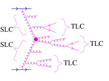
Figure 32: A single parton-parton scattering diagram, with SL and TL cascades, including quarks.

In order to construct the color flow diagram, we remember that in case of a $g\to g+g$ splitting, the emitted gluon may be emitted (with equal probability) on the color side or the anticolor side (see discussion in section 4.3). A possible choice is shown in Fig. 33.

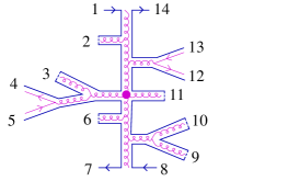
Figure 33: A possible color flow diagram corresponding to Fig. 32.

Following the color flow, always starting and ending with a single arrow, we identify the following chains: 1-2-3-4, then 5-6-7, then 8-9-10-11-12, and finally 13-14.

One should note, as already mentioned several times, that even in the case of multiple scatterings, the remnants are color-white, as are the individual scatterings. In the multiple scattering procedure, where we determine the momenta of all the Pomerons, we also fix the flavors of the “Pomeron ends”. Once these are known, the individual scattering can be treated independently of each other. This is why we discuss here individual scatterings.

4.6 Strings

In the previous sections, we discussed how to construct chains of partons, $j_{1}-j_{2}-...-j_{n}$, where the inner partons are gluons, and the two outer partons, in general, a quark and an antiquark (in any case a $3$ and $\bar{3}$ color representation). These chains of partons are mapped (in a unique fashion) to kinky strings, where each parton corresponds to a kink, and the parton four-momentum defines the kink properties, as already done in earlier EPOS versions, for a detailed discussion see [11]. Let us consider the example of Figs. 32 and 34. Following the color flow, we have identified four chains, namely 1-2-3-4, 5-6-7, 8-9-10-11-12, and 13-14. Each of these chains is mapped to a kinky string, as indicated in Fig. 34.

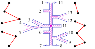
Figure 34: The four color flow chains 1-2-3-4, 5-6-7, 8-9-10-11-12, and 13-14 are mapped to kinky strings (red lines). The black points indicate the kinks.

Each parton corresponds to a kink. The inner kinks correspond to the inner gluons in the chains. The kinks carry the momenta of the corresponding partons. The chain 13-14 corresponds to a string with no inner kinks, so it is a flat (yo-yo) string.

4.7 Heavy quark issues

At each step in the SL cascade, there is the possibility of quark-antiquark production, and in the Born process as well. In the following, we discuss in particular the case of heavy flavor quarks, with the general notation $Q$ for quarks and $\bar{Q}$ for antiquarks. Heavy flavor may be produced in different ways, as shown in Fig. 35.

(a)                          (b)                          (c)                                                          
            

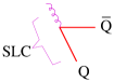
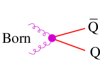
Figure 35: Different possibilities to create heavy flavor, (a) in the spacelike cascade (SLC), (b) in the Born process, (c) in the timelike cascade (TLC).

Starting from a gluon, a $Q-\bar{Q}$ pair may be produced in the SL cascade, as shown in Fig. 35(a), provided the virtuality is large enough. The number of allowed flavors is considered to be depending on the virtuality (variable flavor number scheme). It is also possible to create a $Q-\bar{Q}$ in the Born process, via $g+g\to Q+\bar{Q}$ or $q+\bar{q}\to Q+\bar{Q}$ (for light flavor quarks $q$), as shown in Fig. 35(b), and finally $Q-\bar{Q}$ may be produced in the TL cascade, via $g\to Q+\bar{Q}$, as shown in Fig. 35(c). Let us first consider the $Q-\bar{Q}$ production in the SLC. We may have the situation as shown in Fig. 36(a),

      (a)                                   (b)                                         
      
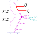
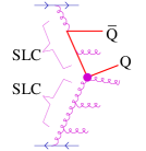
                       (c)                                                                  
      

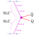
Figure 36: Heavy flavor production (a,b) in the SL cascade and (c) in the Born process. The magenta point indicated the Born process.

where a heavy flavor parton (here a $\bar{Q}$) is emitted, and the corresponding antiparticle (here a $Q$) continues the SLC. But before reaching the Born process, it is emitted, and a gluon continues the SLC. The two heavy flavor partons have in general low transverse momenta. Another possibility is shown in Fig. 36(b), where a heavy flavor parton produced in the SLC “survives” till the Born process, and the latter has most likely the form $Q+l\to Q+l$, with $l$ being a light flavor parton. Other than the production during the SLC, heavy flavor may be produced in the Born process, via $g+g\to Q+\bar{Q}$ or $q+\bar{q}\to Q+\bar{Q}$ (for light flavor quarks $q$), as shown in Fig. 36(c). Finally, heavy flavor may be produced during the timelike cascade, as shown in Fig. 37,

      (a)                                   (b)                                         
      

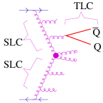
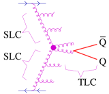
Figure 37: Heavy flavor production in the TL cascade.

initiated either from a TL parton in the SL cascade [Fig. 37(a)], or from an outgoing parton of the Born process (Fig. 37(b)). In the first case, the transverse momenta are in general small.

The next step will be, for a given Feynman diagram, to construct the color flow diagram, as discussed in the previous sections. Let us take the graph of Fig. 37(b), i.e., heavy flavor production during the TLC of an outgoing Born parton. As usual, the gluons are emitted to either side with equal probability, so a possible color flow diagram is the one shown in Fig. 38.

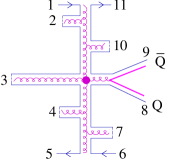
Figure 38: A possible color flow diagram corresponding to the graph of Fig. 37(b)

We identify three chains of partons: 1-2-3-4-5, 6-7-8, and 9-10-11. The initial TL partons (the horizontal blue lines with arrows) or most likely quarks and antiquarks (in any case $3$ and $\bar{3}$ color representations). Let us assume that 3 is a quark, and 6 an antiquark (light flavor, both), then the two chains containing heavy flavor are of the form $\bar{Q}-g-q$ and $\bar{q}-g-Q$, in both cases, the heavy flavor partons are “end partons” in the chains.

These chains of partons are finally mapped (in a unique fashion) to kinky strings, where each parton corresponds to a kink, as shown in Fig. 39.

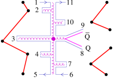
Figure 39: The chains 1-2-3-4-5, 6-7-8, and 9-10-11 are mapped to kinky strings (red lines). The black points indicate the kinks, which carry the parton momenta.

The general mapping procedure (chains of partons to kinky strings) as well as the string decay procedures are described in detail in [11].

5 Summary

We recently introduced new concepts [6], implemented in EPOS4, which allows to consistently accommodate factorization and saturation in high-energy proton-proton and nucleus-nucleus collisions, in a rigorous parallel scattering framework. EPOS4 has a modular structure: the multiple scattering contributions to the total cross section in pp or AA scattering are expressed in terms of (products of) cut Pomeron expressions $G$ (each one representing a single scattering), and the latter ones are related to the “real QCD expressions” $G_{\mathrm{QCD}}$ via some fundamental (new) equation. In other words, $G_{\mathrm{QCD}}$ is the fundamental building block of the multiple scattering framework of EPOS4. In this paper, we provided detailed information about the precise structure of $G_{\mathrm{QCD}}$ and its calculation, based on perturbative QCD, with special care concerning heavy flavor. We discussed the implementation (for the first time in the EPOS framework) of the “backward parton evolution method”, which allows a much better control of the hard processes and comparisons with the “standard” pQCD calculations based on factorization. But compared to those, there are many technical subtleties in our approach, due to the fact that we do the parton evolutions individually for each of the scatterings in a multiple scattering configuration, and this has been discussed in great detail. It is actually the occurrence of singularities for cross section calculations as well as for parton generation which needed to be taken care of. We also discussed the way to transform the partonic multiple scattering structure into strings.

Acknowledgements

KW thanks Sergej Ostapchenko for many helpful discussions concerning the technical aspects of this paper. KW also thanks Tanguy Pierog for useful contributions related to the “deformation function”. BG acknowledges support from ANID PIA/APOYO AFB220004.

APPENDIX

Appendix A Evolution function

A.1 Differential equation for evolution function

It will be useful to have a the differential equation, corresponding to Eq. (46). We may write

$$E_{\mathrm{QCD}}^{ik}\left(x,t_{a},t\right)=\frac{\Delta^{k}(t)}{\Delta^{k}(t_{a})}E_{\mathrm{QCD}}^{ik}\left(x,t_{a},t_{a}\right)$$ (176)

$$\qquad+\sum_{j}\int_{t_{a}}^{t}\frac{dt^{\prime}}{t^{\prime}}\int\frac{dz}{z}\,E_{\mathrm{QCD}}^{ij}\left(\frac{x}{z},t_{a},t^{\prime}\right)\bar{P}_{j}^{k}\!(t^{\prime},z)\,\frac{\Delta^{k}(t)}{\Delta^{k}(t^{\prime})},$$ (177)

with $\Delta^{k}(t)=\Delta^{k}(t_{\mathrm{ref}},t)$, with some arbitrary reference value $t_{\mathrm{ref}}$. We divide by $\Delta^{k}(t)$, to get

$$\frac{E_{\mathrm{QCD}}^{ik}\left(x,t_{a},t\right)}{\Delta^{k}(t)}=\frac{E_{\mathrm{QCD}}^{ik}\left(x,t_{a},t_{a}\right)}{\Delta^{k}(t_{a})}$$ (178)

$$\qquad+\sum_{j}\int_{t_{a}}^{t}\frac{dt^{\prime}}{t^{\prime}}\int\frac{dz}{z}\,\frac{E_{\mathrm{QCD}}^{ij}\left(\frac{x}{z},t_{a},t^{\prime}\right)}{\Delta^{k}(t^{\prime})}\bar{P}_{j}^{k}\!(t^{\prime},z)\,,$$ (179)

then we compute the derivative $\frac{\partial}{\partial t}$ and multiply by $t$, which gives
$$t\frac{\partial}{\partial t}\left\{\frac{E_{\mathrm{QCD}}^{ik}\left(x,t_{a},t\right)}{\Delta^{k}(t)}\right\}=\sum_{j}\int\frac{dz}{z}\,\frac{E_{\mathrm{QCD}}^{ij}\left(\frac{x}{z},t_{a},t\right)}{\Delta^{k}(t)}\bar{P}_{j}^{k}\!(t,z).$$ (180)

A.2 Evolution function theorem

For the proof of Eq. (57) we start from Eq. (180). We first define a matrix $\boldsymbol{E}_{\mathrm{QCD}}^{N}\left(t_{a},t\right)$ with the components

$$E_{\mathrm{QCD}}^{N,ki}\left(t_{a},t\right)=\int_{0}^{1}dx\,x^{N}\,E_{\mathrm{QCD}}^{ik}\left(x,t_{a},t\right),$$ (181)

and we define a vector $\boldsymbol{g}_{N}^{i}(t_{a},t)$ to be the $i^{th}$ column of the matrix $\boldsymbol{E}_{\mathrm{QCD}}^{N}\left(t_{a},t\right)$, divided by $\Delta^{k}(t)$. We further define a matrix $\boldsymbol{\boldsymbol{\gamma}}_{N}(t)$ with elements

$$\boldsymbol{\gamma}_{N}^{kj}(t)=\int_{0}^{1}dx\,x^{N}\,\bar{P}_{j}^{k}\!(t,z).$$ (182)

The Mellin transform of Eq. (180) is then

$$t\frac{\partial}{\partial t}\boldsymbol{g}_{N}^{i}\left(t_{a},t\right)=\boldsymbol{\boldsymbol{\gamma}}_{N}(t)\,\boldsymbol{g}_{N}^{i}\left(t_{a},t\right),$$ (183)

which has the solution

$$\boldsymbol{g}_{N}^{i}\left(t_{a},t\right)=\exp\left(\int_{t_{a}}^{t}\frac{dt^{\prime}}{t^{\prime}}\boldsymbol{\boldsymbol{\gamma}}_{N}\!(t)\right)\boldsymbol{g}_{N}^{i}\left(t_{a},t_{a}\right)$$ (184)

(the exponential of a matrix $M$ is defined by its power series $\sum_{i=0}^{\infty}\frac{1}{i!}M^{i}$). Using $E_{\mathrm{QCD}}^{ik}\left(x,t_{a},t_{a}\right)=\delta(1-x)\delta_{ik},$ we have $\boldsymbol{g}_{N}^{i}\left(t_{a},t_{a}\right)=\boldsymbol{e}_{i}/\Delta^{k}(t)$ (with $\boldsymbol{e}_{i}$ being a vector with the $i^{th}$ component unity and all others zero), and so we get for the matrix $\boldsymbol{E}_{\mathrm{QCD}}^{N}$:

$$\boldsymbol{E}_{\mathrm{QCD}}^{N}\left(t_{a},t\right) =\left\{\boldsymbol{g}_{N}^{1}\left(t_{a},t\right),\boldsymbol{g}_{N}^{2}\left(t_{a},t\right)...\right\}\Delta^{k}(t)$$ (185)

$$=\exp\left(\int_{t_{a}}^{t}\frac{dt^{\prime}}{t^{\prime}}\boldsymbol{\boldsymbol{\gamma}}_{N}\!(t)\right).$$ (186)

Considering $t=t_{b}$, and splitting the integration interval, we get

$$\boldsymbol{E}_{\mathrm{QCD}}^{N}\left(t_{a},t_{b}\right)=\exp\left(\int_{t_{a}}^{t_{c}}\frac{dt^{\prime}}{t^{\prime}}\boldsymbol{\boldsymbol{\gamma}}_{N}\!(t)+\int_{t_{c}}^{t_{b}}\frac{dt^{\prime}}{t^{\prime}}\boldsymbol{\boldsymbol{\gamma}}_{N}\!(t)\right),$$ (187)

which has the structure $e^{A+B}$ with two matrices $A$ and $B$. The Baker-Campbell-Hausdorff formula states

$$e^{A}e^{B}=e^{A+B+X},$$ (188)

with $X=\frac{1}{2}[A,B]+...$, with “…” representing higher commutators of $X$ and $Y$. In leading log accuracy, we can neglect $X$, since it amounts to higher orders in $\alpha_{s}$, and so we get

$$\boldsymbol{E}_{\mathrm{QCD}}^{N}\left(t_{a},t_{b}\right)=\boldsymbol{E}_{\mathrm{QCD}}^{N}\left(t_{c},t_{b}\right)\,\boldsymbol{E}_{\mathrm{QCD}}^{N}\left(t_{a},t_{c}\right),$$ (189)

or, with the corresponding matrix elements,

$$E_{\mathrm{QCD}}^{N,ji}\left(t_{a},t_{b}\right)=\sum_{k}E_{\mathrm{QCD}}^{N,jk}\left(t_{c},t_{b}\right)\,E_{\mathrm{QCD}}^{N,ki}\left(t_{a},t_{c}\right).$$ (190)

The inverse Mellin transformation gives
$$E_{\mathrm{QCD}}^{ij}\left(x,t_{a},t_{b}\right)=\sum_{k}\int\frac{dz}{z}E_{\mathrm{QCD}}^{ik}\left(\frac{x}{z},t_{a},t_{c}\right)E_{\mathrm{QCD}}^{kj}\left(z,t_{c},t_{b}\right)\,.$$ (191) QED.

A.3 Sudakov factor

In this section, we want to prove Eqs. (53,54). The usual form of the DGLAP equations is

$$\mu^{2}\frac{\partial q\left(x,\mu^{2}\right)}{\partial\mu^{2}}=\frac{\alpha_{s}\left(\mu^{2}\right)}{2\pi}$$ (192)

$$\quad\int_{x}^{1}\frac{d\xi}{\xi}\left[P_{qq}(\xi)q\left(x/\xi,\mu^{2}\right)+P_{qg}(\xi)g\left(x/\xi,\mu^{2}\right)\right],$$

$$\mu^{2}\frac{\partial g\left(x,\mu^{2}\right)}{\partial\mu^{2}}=\frac{\alpha_{s}\left(\mu^{2}\right)}{2\pi}$$ (193)

$$\quad\int_{x}^{1}\frac{d\xi}{\xi}\left[\sum_{q,\bar{q}}P_{gq}(\xi)q\left(x/\xi,\mu^{2}\right)+P_{gg}(\xi)g\left(x/\xi,\mu^{2}\right)\right],$$

with LO splitting functions

$$P_{qq}(z)=C_{F}\left[\frac{1+z^{2}}{(1-z)_{+}}+\frac{3}{2}\delta(1-z)\right],$$ (194)

$$P_{qg}(z)=\frac{1}{2}\left[z^{2}+(1-z)^{2}\right],$$ (195)

$$P_{gq}(z)=C_{F}\frac{1+(1-z)^{2}}{z},$$ (196)

$$P_{gg}(z)=2C_{A}\left[\frac{z}{(1-z)_{+}}+\frac{1-z}{z}+z(1-z)\right]$$

$$\qquad+\frac{11C_{A}-2N_{f}}{6}\delta(1-z),$$ (197)

with the usual “+" prescription

$$f(x)_{+}=f(x),\quad 0\leq x<1,$$ (198)

$$\int_{0}^{1}dxg(x)f(x)_{+}=\int_{0}^{1}dxf(x)(g(x)-g(1)).$$ (199)

The “+" and the $\delta$ functions comes from gluon emissions. Without these terms, we obtain the real, or unregularized splitting functions

$$\tilde{P}_{qq}(z)=C_{F}\frac{1+z^{2}}{1-z},$$ (200)

$$\tilde{P}_{gg}(z)=2C_{A}\left[\frac{z}{1-z}+\frac{1-z}{z}+z(1-z)\right],$$ (201)

$$\tilde{P}_{qg}(z)=P_{qg}(z);\quad\tilde{P}_{gq}(z)=P_{gq}(z).$$ (202)

We may use an alternative form of the diagonal splitting functions, namely

$$P_{qq}(z)=C_{F}\left[\frac{1+z^{2}}{(1-z)_{+}}+\frac{3}{2}\delta(1-z)\right]=C_{F}\left(\frac{1+z^{2}}{1-z}\right)_{+},$$ (203)

$$P_{gg}(z) =2C_{A}\left[\frac{z}{(1-z)_{+}}+\frac{1-z}{z}+z(1-z)\right]\qquad\qquad$$

$$\qquad\qquad+\frac{11C_{A}-2N_{f}}{6}\delta(1-z),$$ (204)

$$=\left(2C_{A}\frac{z}{1-z}+C_{A}z(1-z)+\frac{N_{F}}{2}\left(z^{2}+(1-z)^{2}\right)\right)_{+}$$

$$\quad+2C_{A}\frac{1-z}{z}+C_{A}z(1-z)-\frac{N_{F}}{2}\left(z^{2}+(1-z)^{2}\right).$$ (205)

Then we write

$$\int_{x}^{1}\frac{d\xi}{\xi}P_{qq}\left(\frac{x}{\xi}\right)q\left(\xi,\mu^{2}\right)=\int_{x}^{1}\frac{d\xi}{\xi}P_{qq}(\xi)q\left(x/\xi,\mu^{2}\right)$$

$$=\int_{0}^{1}\frac{d\xi}{\xi}P_{qq}(\xi)q\left(x/\xi,\mu^{2}\right)-\int_{0}^{x}\frac{d\xi}{\xi}\tilde{P}_{qq}(\xi)q\left(x/\xi,\mu^{2}\right)$$ (206)

$$=\int_{0}^{1}d\xi\tilde{P}_{qq}(\xi)\left[\frac{1}{\xi}q\left(x/\xi,\mu^{2}\right)-q\left(x,\mu^{2}\right)\right]$$

$$\qquad-\int_{0}^{x}\frac{d\xi}{\xi}\tilde{P}_{qq}(\xi)q\left(x/\xi,\mu^{2}\right)$$ (207)

$$=\int_{1-\varepsilon}^{1}d\xi\tilde{P}_{qq}(\xi)\left[\frac{1}{\xi}q\left(x/\xi,\mu^{2}\right)-q\left(x,\mu^{2}\right)\right]$$

$$+\int_{x}^{1-\varepsilon}\frac{d\xi}{\xi}\tilde{P}_{qq}(\xi)q\left(x/\xi,\mu^{2}\right)$$

$$-q\left(x,\mu^{2}\right)\int_{0}^{1-\varepsilon}d\xi\tilde{P}_{qq}(\xi),$$ (208)

using that fact that in the interval $[0,x]$, we have $f(x)_{+}=f(x)$, and the relation (199). Finally, remarking that for $1-\varepsilon<\xi<1$ and $\varepsilon\to 0$, we get

$$\frac{1}{\xi}q\left(x/\xi,\mu^{2}\right)-q\left(x,\mu^{2}\right)\to 0,$$ (209)

we obtain

$$\int_{x}^{1}\frac{d\xi}{\xi}P_{qq}\left(\frac{x}{\xi}\right)q\left(\xi,\mu^{2}\right)$$ (210)

$$=\int_{x}^{1-\varepsilon}\frac{d\xi}{\xi}\tilde{P}_{qq}(\xi)q\left(x/\xi,\mu^{2}\right)-q\left(x,\mu^{2}\right)\int_{0}^{1-\varepsilon}d\xi\tilde{P}_{qq}(\xi).$$ (211)

The corresponding calculation for the gluon case is

$$\int_{x}^{1}\frac{d\xi}{\xi}P_{gg}\left(\frac{x}{\xi}\right)g\left(\xi,\mu^{2}\right)$$

$$=\int_{0}^{1}\frac{d\xi}{\xi}\left(\frac{2C_{A}\xi}{1-\xi}+C_{A}\xi(1-\xi)+\frac{N_{F}}{2}\left(\xi^{2}+(1-\xi)^{2}\right)\right)_{+}$$

$$\qquad\qquad g\left(x/\xi,\mu^{2}\right)$$

$$-\int_{0}^{x}\frac{d\xi}{\xi}\left(\frac{2C_{A}\xi}{1-\xi}+C_{A}\xi(1-\xi)+\frac{N_{F}}{2}\left(\xi^{2}+(1-\xi)^{2}\right)\right)$$

$$\qquad\qquad g\left(x/\xi,\mu^{2}\right)$$

$$+\int_{x}^{1}\frac{d\xi}{\xi}\left[2C_{A}\frac{1-\xi}{\xi}+C_{A}\xi(1-\xi)-\frac{N_{F}}{2}\left(\xi^{2}+(1-\xi)^{2}\right)\right]$$

$$\qquad\qquad g\left(x/\xi,\mu^{2}\right)$$ (212)

$$\simeq\int_{x}^{1-\varepsilon}\frac{d\xi}{\xi}2C_{A}\left[\frac{\xi}{1-\xi}+\frac{1-\xi}{\xi}+\xi(1-\xi)\right]g\left(x/\xi,\mu^{2}\right)$$

$$-g\left(x,\mu^{2}\right)$$ (213)

$$\int_{\varepsilon}^{1-\varepsilon}d\xi\left(\frac{2C_{A}\xi}{1-\xi}+C_{A}\xi(1-\xi)+\frac{N_{F}}{2}\left(\xi^{2}+(1-\xi)^{2}\right)\right)$$

$$=\int_{x}^{1-\varepsilon}\frac{d\xi}{\xi}\tilde{P}_{gg}(\xi)g\left(x/\xi,\mu^{2}\right)$$ (214)

$$-g\left(x,\mu^{2}\right)\int_{\varepsilon}^{1-\varepsilon}d\xi\left[\frac{1}{2}\tilde{P}_{gg}(\xi)+N_{F}\tilde{P}_{qg}(\xi)\right].$$

Going from Eq. (212) to (213), the integrals

$$g\left(x,\mu^{2}\right)\int_{0}^{\varepsilon}d\xi\Bigg{(}\frac{2C_{A}\xi}{1-\xi}$$ (215)

$$+C_{A}\xi(1-\xi)+\frac{N_{F}}{2}\left(\xi^{2}+(1-\xi)^{2}\right)\Bigg{)}$$

and

$$\int_{1-\varepsilon}^{1}\frac{d\xi}{\xi}\Bigg{[}2C_{A}\frac{1-\xi}{\xi}$$ (216)

$$+C_{A}\xi(1-\xi)-\frac{N_{F}}{2}\left(\xi^{2}+(1-\xi)^{2}\right)\Bigg{]}g\left(x/\xi,\mu^{2}\right)$$

have been neglected. Then, we can write the DGLAP equation as

$$\mu^{2}\frac{\partial q\left(x,\mu^{2}\right)}{\partial\mu^{2}}=\frac{\alpha_{s}\left(\mu^{2}\right)}{2\pi}\int_{x}^{1-\varepsilon}\frac{d\xi}{\xi}$$

$$\qquad\Bigg{[}\tilde{P}_{qq}(\xi)q\left(x/\xi,\mu^{2}\right)+\tilde{P}_{qg}(\xi)g\left(x/\xi,\mu^{2}\right)\Bigg{]}$$

$$\qquad-q\left(x,\mu^{2}\right)\left\{\frac{\alpha_{s}\left(\mu^{2}\right)}{2\pi}\int_{0}^{1-\varepsilon}d\xi\tilde{P}_{qq}(\xi)\right\}\,,$$ (217)

$$\mu^{2}\frac{\partial g\left(x,\mu^{2}\right)}{\partial\mu^{2}}=\frac{\alpha_{s}\left(\mu^{2}\right)}{2\pi}\int_{x}^{1-\varepsilon}\frac{d\xi}{\xi}$$

$$\qquad\left[\sum_{q,\bar{q}}\tilde{P}_{gq}(\xi)q\left(x/\xi,\mu^{2}\right)+\tilde{P}_{gg}(\xi)g\left(x/\xi,\mu^{2}\right)\right]$$

$$\;-g\left(x,\mu^{2}\right)\left\{\frac{\alpha_{s}\left(\mu^{2}\right)}{2\pi}\int_{\varepsilon}^{1-\varepsilon}d\xi\left[\frac{1}{2}\tilde{P}_{gg}(\xi)+N_{F}\tilde{P}_{qg}(\xi)\right]\right\}\,.$$ (218)

Defining
$\displaystyle A_{q}$ $\displaystyle=\frac{\alpha_{s}\left(\mu^{2}\right)}{2\pi}\int_{0}^{1-\varepsilon}d\xi\tilde{P}_{qq}(\xi),$ (219) $\displaystyle A_{g}$ $\displaystyle=\frac{\alpha_{s}\left(\mu^{2}\right)}{2\pi}\int_{\varepsilon}^{1-\varepsilon}d\xi\left[\frac{1}{2}\tilde{P}_{gg}(\xi)+N_{F}\tilde{P}_{qg}(\xi)\right],$ (220)

(representing the expressions in curly brackets in Eqs. (217,218), we get from Eqs. (217,218)

$$\mu^{2}\frac{\partial q\left(x,\mu^{2}\right)}{\partial\mu^{2}}+q\left(x,\mu^{2}\right)A_{q}=\frac{\alpha_{s}\left(\mu^{2}\right)}{2\pi}\int_{x}^{1-\varepsilon}\frac{d\xi}{\xi}$$

$$\qquad\Bigg{[}\tilde{P}_{qq}(\xi)q\left(x/\xi,\mu^{2}\right)+\tilde{P}_{qg}(\xi)g\left(x/\xi,\mu^{2}\right)\Bigg{]}\>,$$ (221)

$$\mu^{2}\frac{\partial g\left(x,\mu^{2}\right)}{\partial\mu^{2}}+g\left(x,\mu^{2}\right)A_{g}=\frac{\alpha_{s}\left(\mu^{2}\right)}{2\pi}\int_{x}^{1-\varepsilon}\frac{d\xi}{\xi}$$

$$\qquad\left[\sum_{q,\bar{q}}\tilde{P}_{gq}(\xi)q\left(x/\xi,\mu^{2}\right)+\tilde{P}_{gg}(\xi)g\left(x/\xi,\mu^{2}\right)\right]\>.$$ (222)

Defining Sudakov factors $\Delta_{g}$ and $\Delta_{q}$ as
$$\Delta_{a}=\exp\left(-\int_{\mu_{0}^{2}}^{\mu^{2}}\frac{dq^{2}}{q^{2}}A_{a}\right),$$ (223) we find for $f_{q}=q$ and $f_{g}=g$:

$$\mu^{2}\frac{\partial}{\partial\mu^{2}}f_{a}(x,\mu^{2})+f_{a}A_{a}=\Delta_{a}\,\mu^{2}\frac{\partial}{\partial\mu^{2}}\left(\frac{f_{a}(x,\mu^{2})}{\Delta_{a}(\mu^{2})}\right).$$ (224)

Reporting this into Eqs. (221) and (222), we get
$\displaystyle\Delta_{q}(\mu^{2})\mu^{2}\frac{\partial}{\partial\mu^{2}}\left\{\frac{q(x,\mu^{2})}{\Delta_{q}(\mu^{2})}\right\}=\frac{\alpha_{s}\left(\mu^{2}\right)}{2\pi}\int_{x}^{1-\varepsilon}\frac{d\xi}{\xi}$ (225) $\displaystyle\qquad\qquad\Bigg{[}\tilde{P}_{qq}(\xi)q\left(x/\xi,\mu^{2}\right)+\tilde{P}_{qg}(\xi)g\left(x/\xi,\mu^{2}\right)\Bigg{]}$ $\displaystyle\Delta_{g}(\mu^{2})\mu^{2}\frac{\partial}{\partial\mu^{2}}\left\{\frac{g\left(x,\mu^{2}\right)}{\Delta_{g}(\mu^{2})}\right\}=\frac{\alpha_{s}\left(\mu^{2}\right)}{2\pi}\int_{x}^{1-\varepsilon}\frac{d\xi}{\xi}$ (226) $\displaystyle\qquad\qquad\left[\sum_{q,\bar{q}}\tilde{P}_{gq}(\xi)q\left(x/\xi,\mu^{2}\right)+\tilde{P}_{gg}(\xi)g\left(x/\xi,\mu^{2}\right)\right],$ which is the DGLAP equation based on unregularized splitting functions, as we use for our $E$ functions, see Eq. (180). We use the convention $P_{i}^{j}=\tilde{P}_{ji}$. Eqs. (223,219,220) agree with Eq. (53,54).

Appendix B Parton-parton cross section formulas

Here we will show how to explicitly do some of the integrations, in order to compute cross sections, starting from Eqs. (45,44).

B.1 Rapidity integral

Here we simplify the expression to get integrated cross sections as rapidity integral. From Eqs. (45,44), we get

$$\sigma_{\mathrm{hard}}^{ij}=\sum_{klmn}\int dy_{3}dy_{4}dp_{3t}^{2}d^{2}p_{4t}\int dx_{1}dx_{2}$$ (227)

$$\qquad E_{\mathrm{QCD}}^{ik}(x_{1},Q_{1}^{2},\mu_{\mathrm{F}}^{2})E_{\mathrm{QCD}}^{jl}(x_{2},Q_{2}^{2},\mu_{\mathrm{F}}^{2})$$

$$\qquad\frac{1}{32s\pi^{2}}\bar{\sum}|\mathcal{M}^{kl\to mn}|^{2}\delta^{4}(p_{1}+p_{2}-p_{3}-p_{4})\frac{1}{1+\delta_{mn}}.$$

Integrating explicitly over $\vec{p}_{4t}$ , which removes

$$\delta^{2}(\vec{p}_{1t}+\vec{p}_{2t}-\vec{p}_{3t}-\vec{p}_{4t}),$$ (228)

and using $d^{2}p_{3t}=d^{2}p_{t}$$=\pi dp_{t}^{2}$, we get

$$\sigma_{\mathrm{hard}}^{ij}=\sum_{klmn}\int dy_{3}dy_{4}dp_{t}^{2}dx_{1}dx_{2}$$

$$\qquad E_{\mathrm{QCD}}^{ik}(x_{1},Q_{1}^{2},\mu_{\mathrm{F}}^{2})E_{\mathrm{QCD}}^{jl}(x_{2},Q_{2}^{2},\mu_{\mathrm{F}}^{2})\>\frac{1}{32s\pi}$$ (229)

$$\qquad\bar{\sum}|\mathcal{M}^{kl\to mn}|^{2}\,\frac{1}{J}\,\delta(P_{\mathrm{in}}^{+}-P_{\mathrm{out}}^{+})\delta(P_{\mathrm{in}}^{-}-P_{\mathrm{out}}^{-})\frac{1}{1+\delta_{mn}},$$

with $J=1/2.$ Here we used the identity

$$\delta^{2}(\vec{x}-\vec{x}_{0})=\frac{1}{J}\delta^{2}(\vec{y}-\vec{y}_{0}),\;J=\left|\frac{\partial(x_{1},x_{2})}{\partial(y_{1},y_{2})}\right|,$$ (231)

valid for any $\vec{x}(\vec{y})$, and in this case used for $x_{1}=E$, $x_{2}=P_{\|}$, $y_{1}=P^{+},$ $y_{2}=P^{-},$ which gives $J=1/2$. The LC momenta are given as $p_{1}^{+}=x_{1}\sqrt{s_{\mathrm{lad}}}$, $p_{1}^{-}=0$, $p_{2}^{+}=0$, $p_{2}^{-}=x_{2}\sqrt{s_{\mathrm{lad}}}$, and for the out-going partons as $p_{3}^{+}=p_{t}e^{y_{3}}$, $p_{3}^{-}=p_{t}e^{-y_{3}}$ and $p_{4}^{+}=p_{t}e^{y_{4}}$, $p_{4}^{-}=p_{t}e^{-y_{4}}$, so we have

$$\delta(P_{\mathrm{in}}^{+}-P_{\mathrm{out}}^{+})=\delta(x_{1}\sqrt{s_{lad}}-p_{t}e^{y_{3}}-p_{t}e^{y_{4}}),$$ (232)

$$\delta(P_{\mathrm{in}}^{-}-P_{\mathrm{out}}^{-})=\delta(x_{2}\sqrt{s_{\mathrm{lad}}}-p_{t}e^{-y_{3}}-p_{t}e^{-y_{4}}),$$ (233)

which gives

$$\delta(P_{\mathrm{in}}^{+}-P_{\mathrm{out}}^{+})=\frac{1}{\sqrt{s_{\mathrm{lad}}}}\delta\left(x_{1}-\frac{1}{2}x_{t}\left(e^{y_{3}}+e^{y_{4}}\right)\right),$$ (234)

$$\delta(P_{\mathrm{in}}^{-}-P_{\mathrm{out}}^{-})=\frac{1}{\sqrt{s_{\mathrm{lad}}}}\delta\left(x_{2}-\frac{1}{2}x_{t}\left(e^{-y_{3}}+e^{-y_{4}}\right)\right),$$ (235)

with $x_{t}=2p_{t}/\sqrt{s_{\mathrm{lad}}}$, and so we get
$\displaystyle\sigma_{\mathrm{hard}}^{ij}=\sum_{klmn}\int dy_{3}dy_{4}dp_{t}^{2}$ $\displaystyle\qquad E_{\mathrm{QCD}}^{ik}(x_{1},Q_{1}^{2},\mu_{\mathrm{F}}^{2})E_{\mathrm{QCD}}^{jl}(x_{2},Q_{2}^{2},\mu_{\mathrm{F}}^{2})$ $\displaystyle\qquad\frac{1}{16\pi s\,s_{\mathrm{lad}}}\bar{\sum}|\mathcal{M}^{kl\to mn}|^{2}\frac{1}{1+\delta_{mn}}\,,$ (236)
with (from integrating over the delta functions)

$$x_{1}=\frac{p_{t}}{\sqrt{s_{\mathrm{lad}}}}\left(e^{y_{3}}+e^{y_{4}}\right),\>x_{2}=\frac{p_{t}}{\sqrt{s_{\mathrm{lad}}}}\left(e^{-y_{3}}+e^{-y_{4}}\right)$$ (237)

and $\delta_{mn}$ accounting for properly counting identical partons.

B.2 LC momentum fraction integral

Here we want to show that $\sigma_{\mathrm{hard}}^{ij}$ in Eq. (236) can be written as an integral over light-cone momentum fractions.

It will be useful to consider quantities in the CMS of the two partons entering the Born process (BornCMS). We may write (with $E=\sqrt{s}/2$)

$$p_{1}= (E,\>E\>,\,\,0\>,0),\quad p_{2}=(E,\>-E\>,\>0\,\,,0),$$ (238)

$$p_{3}= (E,E\cos\theta,E\sin\theta,0),$$ (239)

$$p_{4}= (E,-E\cos\theta,-E\sin\theta,0),$$ (240)

which allows computing

$$t=-\frac{s}{2}(1-\cos\theta),\>u=-\frac{s}{2}(1+\cos\theta).$$ (241)

Using

$$\cos\theta=\frac{(p_{3})_{z}}{(p_{3})_{0}}=\tanh\left(y_{3\,\mathrm{BornCMS}}\right)=\tanh\left(\frac{y_{3}-y_{4}}{2}\right),$$ (242)

and Eq. (237) with $a=1/\sqrt{s_{\mathrm{lad}}}$,

$$x_{1}=ap_{t}\left(e^{y_{3}}+e^{y_{4}}\right),\>x_{2}=ap_{t}\left(e^{-y_{3}}+e^{-y_{4}}\right),$$ (243)

we get the Jacobian matrix

$$\frac{\partial(x_{1},x_{2},\cos\theta)}{\partial(y_{3},y_{4},p_{t}^{2})}=$$ (244)

$$\left(\begin{array}[]{ccc}ap_{t}e^{y_{3}}&ap_{t}e^{y_{4}}&\frac{a}{2p_{t}}\left(e^{y_{3}}+e^{y_{4}}\right)\\ -ap_{t}e^{-y_{3}}&-ap_{t}e^{-y_{4}}&\frac{a}{2p_{t}}\left(e^{-y_{3}}+e^{-y_{4}}\right)\\ \frac{1/2}{\cosh^{2}(\frac{y_{3}-y_{4}}{2})}&\frac{-1/2}{\cosh^{2}(\frac{y_{3}-y_{4}}{2})}&0\end{array}\right),$$ (248)

and the Jacobian determinant

$$J= \frac{a^{2}/4}{\cosh^{2}(\frac{y_{3}-y_{4}}{2})}\Bigg{(}\left|\begin{array}[]{cc}e^{y_{4}}&\left(e^{y_{3}}+e^{y_{4}}\right)\\ -e^{-y_{4}}&\left(e^{-y_{3}}+e^{-y_{4}}\right)\end{array}\right|$$ (251)

$$+\left|\begin{array}[]{cc}e^{y_{3}}&\left(e^{y_{3}}+e^{y_{4}}\right)\\ -e^{-y_{3}}&\left(e^{-y_{3}}+e^{-y_{4}}\right)\end{array}\right|\Bigg{)},$$ (254)

$$= \frac{a^{2}/4}{\cosh^{2}(\frac{y_{3}-y_{4}}{2})}\Bigg{(}e^{y_{4}}\left(e^{-y_{3}}+e^{-y_{4}}\right)+e^{-y_{4}}\left(e^{y_{3}}+e^{y_{4}}\right)$$

$$+e^{y_{3}}\left(e^{-y_{3}}+e^{-y_{4}}\right)+e^{-y_{3}}\left(e^{y_{3}}+e^{y_{4}}\right)\Bigg{)},$$ (255)

$$= \frac{a^{2}/2}{\cosh^{2}(\frac{y_{3}-y_{4}}{2})}\left(e^{y_{3}-y_{4}}+e^{-y_{3}+y_{4}}+1+1\right),$$ (256)

$$= \frac{a^{2}/2}{\cosh^{2}(\frac{y_{3}-y_{4}}{2})}\left(e^{\frac{y_{3}-y_{4}}{2}}+e^{-\frac{y_{3}-y_{4}}{2}}\right)^{2},$$ (257)

$$= 2a^{2}=2/s_{\mathrm{lad}}.$$ (258)

So we get

$$dy_{3}dy_{4}dp_{t}^{2}=\frac{1}{2}s_{\mathrm{lad}}\,dx_{1}dx_{2}d\cos\theta,$$ (259)

and with [from Eq. (241)]

$$dt=\frac{1}{2}s\,d\cos\theta,$$

we find

$$dy_{3}dy_{4}dp_{t}^{2}=\frac{1}{x_{1}x_{2}}dx_{1}dx_{2}dt,$$ (260)

and so, from Eq. (236)

$$\sigma_{\mathrm{hard}}^{ij}=\sum_{klmn}\int dx_{1}dx_{2}dt\,E_{\mathrm{QCD}}^{ik}(x_{1},Q_{1}^{2},\mu_{\mathrm{F}}^{2})E_{\mathrm{QCD}}^{jl}(x_{2},Q_{2}^{2},\mu_{\mathrm{F}}^{2})$$

$$\times\frac{1}{16\pi s^{2}}\bar{\sum}|\mathcal{M}^{kl\to mn}|^{2}\frac{1}{1+\delta_{mn}},$$ (261)

which we may write as
$$\sigma_{\mathrm{hard}}^{ij}\!=\!\!\sum_{klmn}\int\!\!dx_{1}\,dx_{2}\,dt\,E_{\mathrm{QCD}}^{ik}(x_{1},Q_{1}^{2},\mu_{\mathrm{F}}^{2})E_{\mathrm{QCD}}^{jl}(x_{2},Q_{2}^{2},\mu_{\mathrm{F}}^{2})$$ $$\times\frac{\pi\alpha_{s}^{2}}{s^{2}}\left\{\frac{1}{g^{4}}\bar{\sum}|\mathcal{M}^{kl\to mn}|^{2}\right\}\frac{1}{1+\delta_{mn}},$$ (262)
with $\left\{...\right\}$being of the form in which the squared matrix elements are usually tabulated, with $\alpha_{s}=g^{2}/4\pi$. The corresponding differential cross section is

$$\frac{d\sigma_{\mathrm{hard}}^{ij}}{dx_{1}\,dx_{2}\,dt}\!=\!\!\sum_{klmn}E_{\mathrm{QCD}}^{ik}(x_{1},Q_{1}^{2},\mu_{\mathrm{F}}^{2})E_{\mathrm{QCD}}^{jl}(x_{2},Q_{2}^{2},\mu_{\mathrm{F}}^{2})$$

$$\times\frac{\pi\alpha_{s}^{2}}{s^{2}}\left\{\frac{1}{g^{4}}\bar{\sum}|\mathcal{M}^{kl\to mn}|^{2}\right\}\frac{1}{1+\delta_{mn}}.$$ (263)

B.3 Single jet parton-parton cross section

Here we show that $d^{3}\sigma_{\mathrm{hard}}^{ij}/dy\,d^{2}p_{t}$ can be written as a single integral $\int dx...$, where $y$ and $p_{t}$ refer to one outgoing parton (jet).

Again starting from Eq. (44), one may integrate over $\vec{p}_{4}$, to get

$$\frac{d^{3}\sigma_{\mathrm{hard}}^{ij}}{dyd^{2}p_{t}}=\sum_{klmn}\int\!\int\!\!dx_{1}dx_{2}$$ (264)

$$\qquad\,E_{\mathrm{QCD}}^{ik}(x_{1},Q_{1}^{2},\mu_{\mathrm{F}}^{2})E_{\mathrm{QCD}}^{jl}(x_{2},Q_{2}^{2},\mu_{\mathrm{F}}^{2})$$

$$\qquad\frac{1}{32s\pi^{2}}\bar{\sum}|\mathcal{M}^{kl\to mn}|^{2}\frac{1}{1+\delta_{mn}}\frac{1}{E_{4}}\delta(E_{1}+E_{2}-E_{3}-E_{4}),$$

where $y$ and $p_{t}$ refer to particle 3. In the BornCMS, we have (with $E_{3}=E_{4}=E$ and $E_{1}=E_{2}=\sqrt{s}/2$, not yet imposing energy conservation)

$$t=-E\sqrt{s}(1-\cos\theta),\>u=-E\sqrt{s}(1+\cos\theta),$$ (265)

and so

$$\frac{1}{E_{4}}\delta(E_{1}+E_{2}-E_{3}-E_{4})$$

$$\>=\delta\Big{(}E(\sqrt{s}-2E)\Big{)}=\delta\Big{(}\frac{\sqrt{s}}{2}(\sqrt{s}-2E)\Big{)}$$

$$\>=2\delta\Big{(}s-2\sqrt{s}E)\Big{)}=2\delta(s+t+u),$$ (266)

which leads to

$$\frac{d^{2}\sigma_{\mathrm{hard}}^{ij}}{dydp_{t}^{2}}\!=\!\sum_{klmn}\int\!dx_{1}dx_{2}\,E_{\mathrm{QCD}}^{ik}(x_{1},Q_{1}^{2},\mu_{\mathrm{F}}^{2})E_{\mathrm{QCD}}^{jl}(x_{2},Q_{2}^{2},\mu_{\mathrm{F}}^{2})$$

$$\>\times\frac{1}{16\pi s^{2}}\bar{\sum}|\mathcal{M}^{kl\to mn}|^{2}\frac{1}{1+\delta_{mn}}\,s\,\delta(s+t+u).$$ (267)

Using $p_{1}^{+}=x_{1}\sqrt{s_{\mathrm{lad}}}$, $p_{1}^{-}=0$, $p_{3}^{+}=p_{t}e^{y}$, $p_{3}^{-}=p_{t}e^{-y}$, we get

$$t=(p_{1}-p_{3})^{+}(p_{1}-p_{3})^{-}-p_{t}^{2}=-p_{t}x_{1}\sqrt{s_{\mathrm{lad}}}e^{-y}$$ (268)

and with $p_{2}^{-}=x_{2}\sqrt{s_{\mathrm{lad}}}$, $p_{2}^{+}=0$, we find

$$u=(p_{2}-p_{3})^{+}(p_{2}-p_{3})^{-}-p_{t}^{2}=-p_{t}x_{2}\sqrt{s_{\mathrm{lad}}}e^{+y}$$ (269)

and therefore (using $x_{t}=2p_{t}/\sqrt{s_{\mathrm{lad}}}$)

$$s\,\delta(s+t+u)$$ (270)

$$=x_{1}x_{2}\delta\left(x_{1}x_{2}-x_{1}\begin{array}[]{c}\frac{x_{t}}{2}\end{array}e^{-y}-x_{2}\begin{array}[]{c}\frac{x_{t}}{2}\end{array}e^{y}\right)$$ (273)

$$=x_{1}x_{2}\delta\big{(}x(x_{2}-\frac{x_{1}}{x}\begin{array}[]{c}\frac{x_{t}}{2}\end{array}e^{-y})\big{)}$$ (275)

$$=x_{1}x_{2}\frac{1}{x}\delta(x_{2}-\frac{x_{1}}{x}\begin{array}[]{c}\frac{x_{t}}{2}\end{array}e^{-y})$$ (277)

with $x=x_{1}-\begin{array}[]{c}\frac{x_{t}}{2}\end{array}e^{y}$. So we have finally

$$\frac{d^{2}\sigma_{\mathrm{hard}}^{ij}}{dydp_{t}^{2}}=\sum_{klmn}\int dx\,E_{\mathrm{QCD}}^{ik}(x_{1},Q_{1}^{2},\mu_{\mathrm{F}}^{2})E_{\mathrm{QCD}}^{jl}(x_{2},Q_{2}^{2},\mu_{\mathrm{F}}^{2})$$

$$\qquad\times\frac{1}{16\pi s^{2}}\,\bar{\sum}|\mathcal{M}^{kl\to mn}|^{2}\frac{1}{1+\delta_{mn}}\,x_{1}x_{2}\frac{1}{x}$$ (278)

$$\mathrm{\qquad\quad with}\;x_{1}=x+\begin{array}[]{c}\frac{x_{t}}{2}\end{array}e^{y},\,x_{2}=\begin{array}[]{c}\frac{x_{1}}{x}\,\frac{x_{t}}{2}\end{array}e^{-y}.$$ (281)

or
$\displaystyle\frac{d^{2}\sigma_{\mathrm{hard}}^{ij}}{dydp_{t}^{2}}=\sum_{klmn}\int_{b}^{a}dx\,E_{\mathrm{QCD}}^{ik}(x_{1},Q_{1}^{2},\mu_{\mathrm{F}}^{2})E_{\mathrm{QCD}}^{jl}(x_{2},Q_{2}^{2},\mu_{\mathrm{F}}^{2})$ $\displaystyle\qquad\times\frac{\pi\alpha_{s}^{2}}{s^{2}}\left\{\begin{array}[]{c}\frac{1}{g^{4}}\end{array}\bar{\sum}|\mathcal{M}^{kl\to mn}(s,t)|^{2}\right\}\frac{1}{1\!+\!\delta_{mn}}\,x_{1}x_{2}\frac{1}{x}\,,$ (283)
with
$\displaystyle x_{1}=x+\begin{array}[]{c}\frac{p_{t}}{\sqrt{s_{\mathrm{lad}}}}\end{array}e^{y},\,x_{2}=\begin{array}[]{c}\frac{x_{1}}{x}\,\frac{p_{t}}{\sqrt{s_{\mathrm{lad}}}}\end{array}e^{-y},$ (286) $\displaystyle s=x_{1}x_{2}\sqrt{s_{\mathrm{lad}}},\,t=-p_{t}x_{1}\sqrt{s_{\mathrm{lad}}}e^{-y}\,,$ (287) $\displaystyle a=\begin{array}[]{c}\frac{2p_{t}^{2}}{s_{\mathrm{lad}}}\end{array}/(2-\!\!\begin{array}[]{c}\frac{2p_{t}}{\sqrt{s_{\mathrm{lad}}}}\end{array}\!e^{-y}),\>b=1-\!\!\begin{array}[]{c}\frac{p_{t}}{\sqrt{s_{\mathrm{lad}}}}\end{array}\!e^{y},$ (291)
with $\left\{...\right\}$being the form the squared matrix elements are usually tabulated, with $\alpha_{s}=g^{2}/4\pi$, and where the integration limits $a$ and $b$ are obtained from $x_{2}\leq 1$ and $x_{1}\leq 1$. This formula is useful to compute (without Monte Carlo) transverse momentum spectra of produced partons for tests and comparisons.

In the EPOS framework, we have evolution functions with an initial condition $\delta(1-x)$, which forces us to distinguish four cases, namely both-sided, one-sided(lower), one-sided(upper), or no emissions. In the case of both-sided emissions, we use Eq. (283), with $\tilde{E}_{\mathrm{QCD}}^{ab}$ instead of $E_{\mathrm{QCD}}^{ab}$. In case of no emissions on either side, we have $E_{\mathrm{QCD}}^{ab}(x_{i},Q_{i}^{2},\mu_{\mathrm{F}}^{2})=\Delta_{\mathrm{QCD}}^{a}(Q_{i}^{2},\mu_{\mathrm{F}}^{2})\delta(1-x_{i})\delta_{ab}$ on both sides, so $\int\!dx_{1}dx_{2}...$ is trivial, and using $\delta(s+t+u)=\delta(f(y))$ $=\delta\big{(}(y-y_{0})f^{\prime}(y_{0})\big{)}$ $+\delta\big{(}(y+y_{0})f^{\prime}(-y_{0})\big{)}$, with

$$f(y) =s+t+u,$$ (292)

$$=s-x_{1}p_{t}\sqrt{s_{\mathrm{lad}}}e^{-y}-x_{2}p_{t}\sqrt{s_{\mathrm{lad}}}e^{y},$$ (293)

$$=s_{\mathrm{lad}}-p_{t}\sqrt{s_{\mathrm{lad}}}e^{-y}-p_{t}\sqrt{s_{\mathrm{lad}}}e^{y},$$ (294)

$$=s_{\mathrm{lad}}(1-x_{t}\cosh(y)),$$ (295)

and $f^{\prime}(y)=-t+u$, and with $y_{0}$ being the (unique) positive root of $f(y)$, we get (after integrating over $y$)

$$\frac{d^{2}\sigma_{\mathrm{hard}}^{ij}}{dp_{t}^{2}}\!=\!\sum_{mn}\Delta_{\mathrm{QCD}}^{i}(Q_{1}^{2},\mu_{\mathrm{F}}^{2})\Delta_{\mathrm{QCD}}^{j}(Q_{2}^{2},\mu_{\mathrm{F}}^{2})$$

$$\>\times\frac{\pi\alpha_{s}^{2}}{s^{2}}\left\{\begin{array}[]{c}\frac{1}{g^{4}}\end{array}\bar{\sum}|\mathcal{M}^{ij\to mn}|^{2}\right\}\frac{2}{1+\delta_{mn}}\,s_{\mathrm{lad}}\,/|f^{\prime}(y_{0})|.$$ (297)

with $|f^{\prime}(y_{0})|=|t-u|=s-2|t|\approx s_{\mathrm{lad}}$. In case of no emissions on the upper side ($x_{1}=1$), we have t+s+t

$$\frac{d^{2}\sigma_{\mathrm{hard}}^{ij}}{dydp_{t}^{2}}=\sum_{lmn}\Delta_{\mathrm{QCD}}^{i}(Q_{1}^{2},\mu_{\mathrm{F}}^{2})E_{\mathrm{QCD}}^{jl}(x_{2},Q_{2}^{2},\mu_{\mathrm{F}}^{2})$$

$$\qquad\times\frac{\pi\alpha_{s}^{2}}{s^{2}}\left\{\begin{array}[]{c}\frac{1}{g^{4}}\end{array}\bar{\sum}|\mathcal{M}^{il\to mn}|^{2}\right\}\frac{1}{1\!+\!\delta_{mn}}\,x_{2}\frac{1}{x}$$ (299)

$$\qquad\quad\mathrm{with}\>x=1-ae^{y},\,x_{2}=\frac{1}{x}ae^{-y}.$$

In case of no emissions on the lower side ($x_{2}=1$), we have

$$\frac{d^{2}\sigma_{\mathrm{hard}}^{ij}}{dydp_{t}^{2}}=\sum_{kmn}\int dx\,E_{\mathrm{QCD}}^{ik}(x_{1},Q_{1}^{2},\mu_{\mathrm{F}}^{2})\Delta_{\mathrm{QCD}}^{j}(Q_{2}^{2},\mu_{\mathrm{F}}^{2})$$

$$\qquad\times\frac{\pi\alpha_{s}^{2}}{s^{2}}\left\{\begin{array}[]{c}\frac{1}{g^{4}}\end{array}\bar{\sum}|\mathcal{M}^{kj\to mn}|^{2}\right\}\frac{1}{1\!+\!\delta_{mn}}\,x_{1}\frac{1}{x}$$ (301)

$$\qquad\quad\mathrm{with}\>x=1-ae^{-y},\,x_{1}=\frac{1}{x}ae^{y}.$$

We finally mention that the relation

$$x_{1}x_{2}-x_{1}ae^{-y}-x_{2}ae^{y}=0$$ (302)

(from $s+t+u=0)$ not only allows to express $x_{2}$ in terms of $x_{1}$ and $y$ or $x_{1}$ in terms of $x_{2}$ and $y$ (for given $a=\sqrt{p_{t}^{2}/s_{\mathrm{lad}}}$), as

$$x_{2}=\frac{x_{1}ae^{-y}}{x_{1}-ae^{y}},\;x_{1}=\frac{x_{2}ae^{-y}}{x_{2}-ae^{y}},$$ (303)

but also the other way round $y$ in terms of $x_{1}$ and $x_{2}$, as

$$e^{-y}=\frac{2a/x_{1}}{1\pm\sqrt{1-\frac{4a^{2}}{x_{1}x_{2}}}},$$ (304)

or

$$e^{y}=\frac{2a/x_{2}}{1\pm\sqrt{1-\frac{4a^{2}}{x_{1}x_{2}}}},$$ (305)

useful formulas for later applications.

Appendix C Born scattering kinematics: Explicit formulas

Here we will provide explicit formulas for different kinematic quantities and relations related to the Born process, as being used in the numerical procedures.

We consider two partons entering the Born process (let us note them $1$ and $2$), producing two partons (let us note them $3$ and $4$), so altogether we have the elementary process $1+2\to 3+4$. All kinematic formulas depend on the four masses, $m_{1}$, $m_{2}$, $m_{3}$, and $m_{4}$. In order to present explicit formulas for the different cases, we will use the notation

$$case\;m_{1}m_{2}m_{3}m_{4},$$ (306)

so for example “$case\;0000$” represents the case of massless incoming and outgoing partons, like $g+g\to g+g$ or $u+\bar{u}\to g+g$.

C.1 The W variable

Be $E$ and $E^{\prime}$ the modules of the momenta of particles 1 and 3, respectively. We then define $W=4E^{2}$ and $W^{\prime}=4E^{\prime 2}$. We have shown [see Eqs. (70,71)]

$$W=s-2\left(m_{1}^{2}+m_{2}^{2}\right)+\frac{1}{s}\left(m_{1}^{2}-m_{2}^{2}\right)^{2},$$ (307)

$$W^{\prime}=s-2\left(m_{3}^{2}+m_{4}^{2}\right)+\frac{1}{s}\left(m_{3}^{2}-m_{4}^{2}\right)^{2}.$$ (308)

We get for the “interesting cases” explicitly

$$case\;0000\,:W=W^{\prime}=s\>,$$

$$case\;m0m0\,:W=W^{\prime}=\left(s-m^{2}\right)^{2}/s,$$

$$case\;00mm\,:W=s,\,W^{\prime}=s-4m^{2},$$

$$case\;mm00\,:W=s-4m^{2},\,W^{\prime}=s\,,$$ (309)

$$case\;mm\tilde{m}\tilde{m}\,:W=s-4m^{2},\,W^{\prime}=s-4\tilde{m}^{2}$$

$$case\;m\tilde{m}m\tilde{m}\,:W=W^{\prime}=s-2(m^{2}+\tilde{m}^{2})$$

$$\qquad\qquad\qquad\qquad+(m^{2}-\tilde{m}^{2})^{2}/s\,.$$

Here $m$ refers to the charm and $\tilde{m}$ to the bottom quark mass, and $u$, $d$, and $s$ are considered to be massless. These are the formulas used in the code. Essentially all important kinematic relations are expressed in terms of $W$ and $W^{\prime}$.

C.2 Energy limits

The minimum value of the Mandelstam $s$ of the Borm process is [see Eq. (82)]

$$s_{\min}=d\Big{(}1+\sqrt{1-\left((m_{3}^{2}-m_{4}^{2})/d\right)^{2}}\Big{)}\;$$ (310)

$$\mathrm{with}\quad d=m_{3}^{2}+m_{4}^{2}+2\,p_{t\,\mathrm{min}}^{2}.$$

For the “interesting cases”, we get for $s_{\min}$ :

$$0000\,:\;\quad 4\,p_{t\,\mathrm{min}}^{2},$$ (311)

$$m0m0\,:\quad d\left(1+\sqrt{1-m^{4}/d^{2}}\right),$$ (312)

$$\qquad\qquad\qquad\mathrm{with\>d=m^{2}+2\,p_{t\,\mathrm{min}}^{2}},$$

$$00mm\,:\quad 4\Big{(}m^{2}+p_{t\,\mathrm{min}}^{2}\Big{)}\,,$$ (313)

$$mm00\,:\quad 4\,p_{t\,\mathrm{min}}^{2}\,,$$ (314)

$$mm\tilde{m}\tilde{m}\,:\quad 4(\tilde{m}^{2}+p_{t\,\mathrm{min}}^{2})\,,$$ (315)

$$m\tilde{m}m\tilde{m}\,:\,d\Big{(}1+\sqrt{1-\left((m^{2}-\tilde{m}^{2})/d\right)^{2}}\Big{)}\,,$$ (316)

$$\qquad\qquad\qquad\mathrm{with\>d=m^{2}+\tilde{m}^{2}+2\,p_{t\,\mathrm{min}}^{2}\,.}$$

C.3 The variable t

The module of the Mandelstam variable $t$ is given as [see Eq. (84)]

$$|t|=\frac{1}{2}\,\Big{(}\,\sqrt{W+4m_{1}^{2}}\sqrt{W^{\prime}+4m_{3}^{2}}-2(m_{1}^{2}+m_{3}^{2})\qquad$$

$$\qquad\qquad\qquad\mp\sqrt{W}\sqrt{W^{\prime}-4p_{t}^{2}}\,\Big{)},$$ (317)

the “$\mp$” referring to respectively $p_{z}\geq 0$ and $p_{z}\leq 0$. For the different cases, we have

$$m0m0\,:\;|t|=\frac{W}{2}\!\Big{(}\!1\mp\sqrt{1-\frac{4p_{t}^{2}}{W}}\Big{)},$$ (318)

$$00mm\,:\;|t|=\frac{W}{2}\!\Big{(}\!1\mp\sqrt{1-4\frac{p_{t}^{2}+m^{2}}{W}}\Big{)}\!-\!m^{2},$$ (319)

$$mm00\,:\;|t|=\frac{W}{2}\!\Big{(}\!1\mp\sqrt{1-4\frac{p_{t}^{2}-m^{2}}{W}}\Big{)}\!+\!m^{2},$$ (320)

$$mm\tilde{m}\tilde{m}\,:\,|t|=\frac{W}{2}\Big{(}1\mp\sqrt{1-4\frac{p_{t}^{2}-m^{2}+\tilde{m}^{2}}{W}}\,\Big{)}$$

$$\qquad\qquad\qquad\qquad\qquad\qquad\qquad+m^{2}-\tilde{m}^{2}$$ (321)

$$m\tilde{m}m\tilde{m}\,:\,|t|=\frac{W}{2}\!\Big{(}\!1\mp\sqrt{1-\frac{4p_{t}^{2}}{W}}\,\Big{)}.$$ (322)

From Eq. (317), we get

$$|t|_{\mathrm{min/max}}\!=\!\frac{1}{2}\!\Big{(}\!\!\sqrt{W+4m_{1}^{2}}\sqrt{W^{\prime}+4m_{3}^{2}}-2(m_{1}^{2}+m_{3}^{2})$$

$$\qquad\mp\sqrt{W}\sqrt{W^{\prime}-4p_{t\,\min}^{2}}\,\Big{)}.$$ (323)

Considering the different cases, we get for the quantities $|t|_{\mathrm{min/max}}$ :

$$m0m0\,:\;\frac{W}{2}\,\Bigg{(}1\mp\sqrt{1-4p_{t\,\mathrm{min}}^{2}/W}\,\Bigg{)},$$ (324)

$$00mm\,:\;\frac{W}{2}\Big{(}1\mp\sqrt{1-4(p_{t\,\mathrm{min}}^{2}+m^{2})/W}\,\Big{)}-m^{2},\qquad$$ (325)

$$mm00\,:\;\frac{W}{2}\Big{(}1\mp\sqrt{1-4(p_{t\,\min}^{2}-m^{2})/W}\,\Big{)}+m^{2},$$ (326)

$$mm\tilde{m}\tilde{m}\,:\frac{W}{2}\Big{(}1\mp\sqrt{1-4\frac{p_{t\,\min}^{2}-m^{2}+\tilde{m}^{2}}{W}}\,\Big{)}$$

$$\qquad\qquad\qquad\qquad\qquad\qquad\qquad\qquad+m^{2}-\tilde{m}^{2},$$ (327)

$$m\tilde{m}m\tilde{m}\,:\frac{W}{2}\,\Big{(}1\mp\sqrt{1-4p_{t\,\min}^{2}/W}\,\Big{)}\,.$$ (328)

Using the identity

$$\Big{(}1-\sqrt{1-C}\,\Big{)},$$ (329)

$$=\frac{C\Big{(}1-\sqrt{1-C}\,\Big{)}}{\Big{(}1+\sqrt{1-C}\,\Big{)}\Big{(}1-\sqrt{1-C}\,\Big{)}},$$ (330)

$$=\frac{C}{\Big{(}1+\sqrt{1-C}\,\Big{)}},$$ (331)

the latter expression being better for numerical purposes when $C\ll 1$, we get for $|t|_{\mathrm{min}}$ :

$$m0m0:\,\frac{2p_{t\,\mathrm{min}}^{2}}{1+\sqrt{1-4p_{t\,\mathrm{min}}^{2}/W}},$$ (332)

$$00mm:\,\frac{2(p_{t\,\mathrm{min}}^{2}+m^{2})}{1+\sqrt{1-4(p_{t\,\mathrm{min}}^{2}+m^{2})/W}}-m^{2},\quad$$ (333)

$$mm00:\,\frac{2(p_{t\,\mathrm{min}}^{2}-m^{2})}{1+\sqrt{1-4(p_{t\,\mathrm{min}}^{2}-m^{2})/W}}+m^{2},\quad$$ (334)

$$mm\tilde{m}\tilde{m}\,:\frac{2(p_{t\,\min}^{2}-m^{2}+\tilde{m}^{2})}{1+\sqrt{1-4(p_{t\,\min}^{2}-m^{2}+\tilde{m}^{2})/W}}$$

$$\qquad\qquad\qquad\qquad\qquad\qquad\qquad+m^{2}-\tilde{m}^{2},$$ (335)

$$m\tilde{m}m\tilde{m}\,:\frac{2p_{t\,\mathrm{min}}^{2}}{1+\sqrt{1-4p_{t\,\mathrm{min}}^{2}/W}}.$$ (336)

C.4 The limit t_max+

We define the maximum value $|t|_{\mathrm{max+}}$ of $|t|$ with $p_{z}\geq 0$ [see Eq. (87)], i.e.,

$$|t|_{\mathrm{max+}}=\frac{1}{2}\,\Big{(}\,\sqrt{W+4m_{1}^{2}}\sqrt{W^{\prime}+4m_{3}^{2}}-2(m_{1}^{2}+m_{3}^{2})\Big{)}.$$ (337)

For the different cases, we get

$$m0m0:\>|t|_{\mathrm{max+}}=\frac{W}{2}=\frac{\left(s-m\text{\texttwosuperior}\right)^{2}}{2\,s},$$ (338)

$$00mm:\>|t|_{\mathrm{max+}}=\frac{s}{2}-m^{2},$$ (339)

$$mm00:\>|t|_{\mathrm{max+}}=\frac{s}{2}-m^{2},$$ (340)

$$mm\tilde{m}\tilde{m}\,:|t|_{\mathrm{max+}}=\frac{s}{2}-m^{2}-\tilde{m}^{2},$$ (341)

$$m\tilde{m}m\tilde{m}\,:|t|_{\mathrm{max+}}=\frac{W}{2}\,.$$ (342)

C.5 Transverse momentum for given t

The general formula is [see Eq. (85)]

$$p_{t}^{2}=\frac{W^{\prime}}{4}-\frac{1}{W}\,\Big{(}\,|t|-\frac{1}{2}\sqrt{W+4m_{1}^{2}}\sqrt{W^{\prime}+4m_{3}^{2}}$$

$$\qquad\qquad\qquad+m_{1}^{2}+m_{3}^{2}\,\Big{)}^{2}.$$ (343)

For the different cases, we get

$$m0m0:\>p_{t}^{2}=|t|\Big{(}1-\frac{|t|}{W}\Big{)}\,,$$ (344)

$$00mm:\>p_{t}^{2}=\Big{(}|t|+m^{2}\Big{)}\Big{(}1-\frac{|t|+m^{2}}{W}\Big{)}-m^{2},$$ (345)

$$mm00:\>p_{t}^{2}=\Big{(}|t|-m^{2}\Big{)}\Big{(}1-\frac{|t|-m^{2}}{W}\Big{)}+m^{2},$$ (346)

$$mm\tilde{m}\tilde{m}\,:p_{t}^{2}=\Big{(}|t|-m^{2}+\tilde{m}^{2}\Big{)}\Big{(}1-\frac{|t|-m^{2}+\tilde{m}^{2}}{W}\Big{)}$$

$$\qquad\qquad\qquad\qquad\qquad\qquad\qquad\qquad+m^{2}-\tilde{m}^{2},$$ (347)

$$m\tilde{m}m\tilde{m}\,:p_{t}^{2}=|t|\Big{(}1-\frac{|t|}{W}\Big{)}\,.$$ (348)

References

- [1] J. Collins, D. Soper, and G. Sterman, in Perturbative Quantum Chromodynamics, edited by A.H. Mueller, World Scientific, Singapore (1989).
- [2] R. Ellis, W. Stirling, and B. Webber, in QCD and Collider Physics, Cambridge Monographs on Particle Physics, Nuclear Physics and Cosmology, Cambridge University Press, Cambridge (1996).
- [3] D. Gross and F. Wilczek, Physical Review Letters 30, 1343 (1973).
- [4] H. Politzer, Physical Review Letters 30, 1346 (1973).
- [5] CMS, V. Khachatryan et al., JHEP 09, 091 (2010), 1009.4122.
- [6] K. Werner, http://arxiv.org/abs/2301.12517.
- [7] V. N. Gribov, Zh. Eksp. Teor. Fiz. 53, 654 (1967).
- [8] V. N. Gribov, Sov. Phys. JETP 29, 483 (1969).
- [9] V. N. Gribov and L. N. Lipatov, Sov. J. Nucl. Phys. 15, 438 (1972).
- [10] V. A. Abramovsky, V. N. Gribov, and O. V. Kancheli, Yad. Fiz. 18, 595 (1973).
- [11] H. J. Drescher, M. Hladik, S. Ostapchenko, T. Pierog, and K. Werner, Phys. Rept. 350, 93 (2001), hep-ph/0007198.
- [12] G. Altarelli and G. Parisi, Nuclear Physics B. 126, 298 (1977).
- [13] Y. L. Dokshitzer, Sov. Phys. JETP 46, 641 (1977).
- [14] Multiple Parton Interactions at the LHC, edited by Paolo Bartalini and Jonathan Richard Gaunt, World Scientific, ISBN: 978-981-3227-75-0 (2018).
- [15] B. Guiot, Heavy-quark production with -factorization: The importance of the sea-quark distribution, Phys. Rev. D 99 (2019) no.7, 074006.
- [16] B. Guiot and A. van Hameren, D and B-meson production using kt-factorization calculations in a variable-flavor-number scheme, Phys. Rev. D 104 (2021) no.9, 094038
- [17] S. Dulat et al., Physical Review D 93 (2016).
- [18] ZEUS, M. Derrick et al., Z. Phys. C72, 399 (1996), hep-ex/9607002.
- [19] H1 Collaboration, Abt et al., Z. Phys. C63, 377 (1994).
- [20] H1 Collaboration, Aid et al., Nucl. Phys. B470, 3 (1996).
- [21] H1 Collaboration, Adlhoff et al., Nucl. Phys. B485, 3 (1996).
- [22] ATLAS, M. Aaboud et al., JHEP 05, 195 (2018), 1711.02692.
- [23] M. Cacciari et al., JHEP 10, 137 (2012), 1205.6344.
- [24] ALICE, B. Abelev et al., JHEP 01, 128 (2012), 1111.1553.