The Quasinormal Modes and Isospectrality of Bardeen (Anti-) de Sitter Black Holes

Abstract

Black holes (BHs) exhibiting coordinate singularities but lacking essential singularities throughout the entire spacetime are referred to as regular black holes (RBHs). The initial formulation of RBHs was presented by Bardeen, who considered the Einstein equation coupled with a nonlinear electromagnetic field. In this study, we investigate the gravitational perturbations, including the axial and polar sectors, of the Bardeen (Anti-) de Sitter black holes. We derive the master equations with source terms for both axial and polar perturbations, and subsequently compute the quasinormal modes (QNMs) through numerical methods. For the Bardeen de Sitter black hole, we employ the 6th-order WKB approach. The numerical results reveal that the isospectrality is broken in this case. Conversely, for Bardeen Anti-de Sitter black holes, the QNM frequencies are calculated by using the HH method.

I Introduction

Over these years, the gravitational wave searches for the coalescence of compact binaries LIGO and the shadow images captured by the Event Horizon Telescope ETH1 ; ETH2 explicitly give the evidence to the existence of BHs. In general relativity, essential singularities are present in BHs, which cannot be eliminated by coordinate transformation. Modern physics tries to construct a complete theory of quantum gravity, and understand the microscopic mechanism of BHs. However, the description of the essential singularity has encountered enormous difficulties. To overcome this problem, one can consider the BHs without essential singularities are known as regular black holes. Comparing with those of singular black holes, the regular black hole have some new phenomena, and which attract much attention recently miao . This kind of solutions was first proposed by Bardeen Bardeen . Ayón-Beato and García found that, to obtain a regular black hole solution, the energy-momentum tensor should be the gravitational field of some magnetic monopole generated by a specific form of nonlinear electrodynamics EAAG1 ; EAAG2 ; EAAG3 . Since then, numerous researchers have contributed various singularity-free solutions regular1 ; regular2 ; regular3 ; regular4 ; regular5 ; regular6 .

In the context of binary black holes coalescence, the process can be divided into three distinct stages: inspiral, merge and ringdown. Each stage is calculated by different methods. The inspiral can be discussed by the post-Newtonian approximation, and the merge is always calculated by numerical calculation. The final stage is equivalent to making a perturbation to an equilibrium state of the black hole. This stage corresponds to damped oscillations with complex frequencies, which always depend only on black hole properties, like mass, charge and angular momentum. These modes are called quasinormal modes (QNMs). The gravitational perturbation equations for the axial sector of Schwarzschild spacetime were initially formulated by Regge and Wheeler ReggeWheeler1957 , and later extended to the polar sector by Zerilli Zerilli1970PRL ; Zerilli1970PRD . Extensive research has been dedicated to numerically determining the quasinormal frequencies ($\omega$) for various scenarios. It is well-established that the axial and polar gravitational perturbations of asymptotically flat spacetime, such as those associated with Schwarzschild or Reissner-Nordstrom BHs, exhibit isospectrality chandrasekharbook . Conversely, the investigation of quasinormal modes in asymptotically Anti-de Sitter (AdS) spacetime has attracted significant interest due to the AdS/CFT duality Chan ; HH . Numerical investigations have revealed a distinct parity splitting phenomenon for Schwarzschild-AdS BHs Cardoso2001 . Furthermore, in addition to their classical properties, quasinormal modes also exhibit intriguing quantum characteristics inherent to BHs Hod1998 ; Maggiore2008 .

After the Bardeen solution has been presented, many works focused on the perturbation problem of the Bardeen BHs. The QNM due to the neutral or charged scalar field perturbation for regular black hole have been discussed in Ref. Fernando2012 ; Flachi2013 . Ulhoa investigate the axial gravitational perturbations of a regular black hole Ulhoa2014 . To investigate the stability of nonlinear electrodynamics black holes, Moreno and Sarbach derive the perturbation equations Moreno2003 . Based on this result, Chaverra et al. calculate the QNMs of black hole in nonlinear electrodynamics, and find that there exist a parity splitting for the alternative model to the Bardeen black hole Chaverra . Further, Toshmato et al. studied the electromagnetic perturbation of black hole coupled with nonlinear electrodynamics, and their results show a correspondence between the axial and polar parts of electromagnetic perturbations of electrically charged or magnetically charged black hole Toshmato1 ; Toshmato2 . The Dirac QNMs of regular black hole was also investigated in Li2013 .

The Bardeen BH with cosmological constant was initially introduced by Fernando Fernando2016 . In this study, we derive the master variables and corresponding master equations for the gravitational perturbations of Bardeen (Anti-) de Sitter BHs, employing the so-called A-K notation. Our analysis encompasses both the axial (odd-parity) and polar (even-parity) sectors. Subsequently, we numerically compute the QNMs, with necessary analysis. The structure of the paper is outlined as follows: In the subsequent section, we provide a brief overview of the Bardeen BH solution and the construction of master equations for (axial and polar) gravitational perturbations. Section III focuses on the study of QNMs for the Bardeen de Sitter BH utilizing the 6th-order WKB approach. Additionally, we present a comparative discussion regarding the quasinormal frequency splitting phenomenon. Moving on to Section IV, we employ the HH method to calculate the QNMs of the Bardeen Anti-de Sitter BH. Finally, Section V is dedicated to summarizing our findings and providing a comprehensive discussion. Throughout our paper, we choose $c=G=1$ and ignore the factor $\kappa=8\pi$ in gravitational equations.

II Gravitational Perturbation of Bardeen (Anti-) de Sitter Black Hole

First we briefly introduce the Bardeen de Sitter BH following the work in Ref. Fernando2016 , the action is given by

$$S=\int d^{4}x\sqrt{-g}\left[\frac{\left(R-2\Lambda\right)}{16\pi}-\frac{1}{4\pi}\mathcal{L}(F)\right],$$ (1)

where $\mathcal{L}(F)=\frac{3}{2\alpha q^{2}}\left(\frac{\sqrt{2q^{2}F}}{1+\sqrt{2q^{2}F}}\right)^{5/2}$ is the Lagrangian of the nonlinear electromagnetic field strength $F$, and $R$, $\Lambda$ are the scalar curvature, the cosmological constant, respectively. The parameter $\alpha$ in $\mathcal{L}(F)$ is related to the magnetic charge $q$ and the mass $M$ of the space time as follows: $\alpha=q/2M$. The field strength $F$ can be written as

$$F=\frac{1}{4}F_{\mu\nu}F^{\mu\nu}$$ (2)

where $F_{\mu\nu}=\nabla_{\mu}A_{\nu}-\nabla_{\nu}A_{\mu}$. The only non-vanish component of $F_{\mu\nu}$ for spherically symmetric spacetime is $F_{23}=q\sin\theta$, and then $F=q^{2}/2r^{4}$.

Taking the variation of the action, the equation of motion can be expressed as

$$R_{\mu\nu}-\frac{1}{2}Rg_{\mu\nu}+\Lambda g_{\mu\nu}=2\left(\frac{\partial\mathcal{L}(F)}{\partial F}F_{\mu\lambda}F_{\nu}\hskip 0.28453pt^{\lambda}-g_{\mu\nu}\mathcal{L}(F)\right)$$

$$\nabla_{\mu}\left(\frac{\partial\mathcal{L}(F)}{\partial F}F^{\nu\mu}\right)=0,$$ (3)

The static spherically symmetric solution is given by Fernando2016

$$ds^{2}=-f(r)dt^{2}+f(r)^{-1}dr^{2}+r^{2}\left(d\theta^{2}+\sin^{2}\theta d\varphi^{2}\right)$$ (4)

where $f(r)=1-\frac{2Mr^{2}}{(r^{2}+q^{2})^{\frac{3}{2}}}-\frac{\Lambda r^{2}}{3}$, here $M$, $q$ are the total mass and the magnetic charge of the Bardeen de Sitter BH. The $\Lambda>0$ case represents the Bardeen de Sitter BH, and the $\Lambda<0$ case represents the Bardeen Anti-de Sitter BH.

The decomposition of perturbed metric was first presented by Regge and Wheeler. Considering that the perturbed metric can be written as

$$g_{ab}=\bar{g}_{ab}+h_{ab}$$ (5)

where $\bar{g}_{ab}$ denote the metric of the background spacetime. For spherically symmetric spacetime, it is well-known that $h_{ab}$ can be decomposed to the axial part and polar part under the Regge-Wheeler gauge. In this paper, we use A-K notation to decompose $h_{ab}$ Thompson2016 , which helps to give the perturbed source terms. Note that when calculating the QNMs, we do not need the source term. However, here we present the master equation with source term, which can provide some basis to study the self-force or extreme mass ratio inspiral problems for Bardeen (Anti-)de Sitter black hole. Considering that the complete basis on the two-sphere are constructed by 1-scalar spherical harmonic, $Y_{lm}=Y_{lm}(\theta,\varphi)$, three pure-spin vector harmonics and six tensor harmonics Thorne1980 . The vector harmonics are defined as

$$Y_{a}^{E,lm}=r\nabla_{a}Y^{lm},~{}~{}~{}~{}Y_{a}^{B,lm}=r\epsilon_{ab}\hskip 0.28453pt^{c}n^{b}\nabla_{c}Y^{lm},~{}~{}~{}~{}Y_{a}^{R,lm}=n_{a}Y^{lm},$$

and the tensor harmonics are defined as

$$T_{ab}^{T0,lm} = \Omega_{ab}Y^{lm},~{}~{}~{}~{}T_{ab}^{L0,lm}=n_{a}n_{b}Y^{lm},$$

$$T_{ab}^{E1,lm} = r~{}n_{(a}\nabla_{b)}Y^{lm},~{}~{}~{}~{}T_{ab}^{B1,lm}=r~{}n_{(a}\epsilon_{b)c}\hskip 0.28453pt^{d}n^{c}\nabla_{d}Y^{lm},$$

$$T_{ab}^{B2,lm} = r^{2}\Omega_{(a}\hskip 0.28453pt^{c}\epsilon_{b)e}\hskip 0.28453pt^{d}n^{e}\nabla_{c}\nabla_{d}Y^{lm},$$

$$T_{ab}^{E2,lm} = r^{2}\left(\Omega_{a}\hskip 0.28453pt^{c}\Omega_{b}\hskip 0.28453pt^{d}-\frac{1}{2}\Omega_{ab}\Omega^{cd}\right)\nabla_{c}\nabla_{d}Y^{lm}.$$ (7)

where $v_{a}=(-1,0,0,0)$ and $n_{a}=(0,1,0,0)$ are two orthogonal co-vectors, $\Omega_{ab}$ is the projection operator defined as $\Omega_{ab}=r^{2}\text{diag}(0,0,1,\sin^{2}\theta)$, and $\epsilon_{abc}$ represent the spatial Levi-Civita tensor $\epsilon_{abc}\equiv v^{d}\epsilon_{dabc}$. Now, $h_{ab}$ can be decomposed as

$$h_{ab}^{lm} =\mathrm{A~{}}v_{a}v_{b}Y^{lm}+2\mathrm{B~{}}v_{(a}Y_{b)}^{E,lm}+2\mathrm{C~{}}v_{(a}Y_{b)}^{B,lm}+2\mathrm{D~{}}v_{(a}Y_{b)}^{R,lm}$$

$$~{}~{}~{}~{}+\mathrm{E~{}}T^{T0,lm}_{ab}+\mathrm{F~{}}T_{ab}^{E2,lm}+\mathrm{G~{}}T^{B2,lm}_{ab}+2\mathrm{H~{}}T^{E1,lm}_{ab}$$

$$~{}~{}~{}~{}+2\mathrm{J~{}}T^{B1,lm}_{ab}+\mathrm{K~{}}T^{L0,lm}_{ab},$$ (8)

where coefficients of each term in the above equation are all scalar functions of $t$ and $r$. Hence, the polar part and the axial part of $h_{ab}$ can be written as

$$h_{ab}^{polar}=\left(\begin{array}[]{cccc}\mathrm{A}Y^{lm}&-\mathrm{D}Y^{lm}&-r\mathrm{B}\partial_{\theta}Y^{lm}&-r\mathrm{B}\partial_{\phi}Y^{lm}\\ Sym&\mathrm{K}Y^{lm}&-r\mathrm{H}\partial_{\theta}Y^{lm}&r\mathrm{H}\partial_{\phi}Y^{lm}\\ Sym&Sym&r^{2}~{}\mathrm{Z}^{lm}&r^{2}\mathrm{F}X^{lm}\\ Sym&Sym&Sym&r^{2}\sin^{2}\theta~{}\mathrm{Z}^{lm}\end{array}\right)$$ (13)

$$h_{ab}^{axial}=\left(\begin{array}[]{cccc}0&0&r~{}csc\theta\mathrm{C}\partial_{\phi}Y^{lm}&-r~{}sin\theta\mathrm{C}\partial_{\theta}Y^{lm}\\ 0&0&-r~{}csc\theta\mathrm{J}\partial_{\phi}Y^{lm}&r~{}\sin\theta\mathrm{J}\partial_{\theta}Y^{lm}\\ Sym&Sym&-r^{2}csc\theta\mathrm{G}X^{lm}&r^{2}\sin\theta\mathrm{G}W^{lm}\\ Sym&Sym&Sym&r^{2}\sin\theta~{}\mathrm{G}X^{lm}\end{array}\right)$$ (18)

where

$$\mathrm{W}^{lm} = \left[\partial_{\theta}^{2}+\frac{1}{2}l\left(l+1\right)\right]Y^{lm}$$

$$\mathrm{X}^{lm} = \left[\partial_{\theta}\partial_{\phi}-cot\theta\partial_{\phi}\right]Y^{lm}$$

$$\mathrm{Z}^{lm} = \left(\mathrm{E}Y^{lm}+\mathrm{F}W^{lm}\right)$$ (19)

Assuming that the value of charge $q$ is fixed, taking the variation of Eq. (II) we obtain

$$E_{ab} =\Box h_{ab}+\nabla_{a}\nabla_{b}h^{c}_{~{}c}-2\nabla_{(a}\nabla^{c}h_{b)c}+2R^{~{}c~{}d}_{a~{}b}h_{cd}$$

$$~{}~{}~{}~{}-(R_{a}\hskip 0.28453pt^{c}h_{bc}+R_{b}\hskip 0.28453pt^{c}h_{ac})+g_{ab}(\nabla^{c}\nabla^{d}h_{cd}-\Box h^{d}_{~{}d})$$

$$~{}~{}~{}~{}-g_{ab}R^{cd}h_{cd}+Rh_{ab}-2\Lambda h_{ab}+2\delta T^{\text{Bardeen}}_{ab}$$ (20)

where

$$\delta T^{\text{Bardeen}}_{ab}=2\delta\left(\frac{\partial\mathcal{L}(F)}{\partial F}F_{\mu\lambda}F_{\nu}\hskip 0.28453pt^{\lambda}-g_{\mu\nu}\mathcal{L}(F)\right)$$ (21)

Project the above equation to the A-K directions, one can get the projection equations $E_{\mathrm{A}}-E_{\mathrm{K}}$. The explicit expression of $E_{\mathrm{A}}-E_{\mathrm{K}}$ will be placed in Appendix A.

For spherically symmetric spacetimes, there are several gauge choices ReggeWheeler1957 . In this paper, we choose the RW gauge, i.e., choose the gauge vector $\xi_{a}$ as

$$\xi_{a} =\left(rB+\frac{r^{2}}{2}\frac{\partial}{\partial t}F\right)v_{a}Y^{lm}+\left(rH-\frac{r}{2}\frac{\partial}{\partial r}F\right)Y^{R,lm}_{a}$$

$$~{}~{}~{}~{}+\frac{r}{2}FY^{E,lm}_{a}+\frac{r}{2}GY^{B,lm}_{a}$$ (22)

which yields $B=F=H=G=0$. Then, the polar and the axial sectors of $h_{ab}$ become

$$h_{ab}^{polar}=\left(\begin{array}[]{cccc}\mathrm{A}Y^{lm}&-\mathrm{D}Y^{lm}&0&0\\ -\mathrm{D}Y^{lm}&\mathrm{K}Y^{lm}&0&0\\ 0&0&r^{2}~{}\mathrm{E}Y^{lm}&0\\ 0&0&0&r^{2}\sin^{2}\theta~{}\mathrm{E}Y^{lm}\end{array}\right)$$ (27)

$$h_{ab}^{axial}=\left(\begin{array}[]{cccc}0&0&r~{}csc\theta\mathrm{C}\partial_{\phi}Y^{lm}&-r~{}sin\theta\mathrm{C}\partial_{\theta}Y^{lm}\\ 0&0&-r~{}csc\theta\mathrm{J}\partial_{\phi}Y^{lm}&r~{}\sin\theta\mathrm{J}\partial_{\theta}Y^{lm}\\ Sym&Sym&0&0\\ Sym&Sym&0&0\end{array}\right)$$ (33)

Then, we construct the master variables and master equations for axial part or even part respectively. For axial part, let

$$\psi^{(-)}=f\mathrm{J}$$ (35)

and $\psi^{(-)}$ satisfied

$$\left(f^{2}\frac{\partial^{2}}{\partial r^{2}}-\frac{\partial^{2}}{\partial t^{2}}+f^{\prime}f\frac{\partial}{\partial r}-V^{(-)}\right)\psi^{(-)}=S^{(-)}$$ (36)

with

$$V^{(-)}=\frac{f}{r^{2}}\left(-2+\lambda+2r^{2}\Lambda+2f+rf^{\prime}+r^{2}f^{\prime\prime}+4r^{2}\kappa\mathcal{L}\right).$$

and

$$S^{(-)}=f^{2}E_{\mathrm{J}}-\frac{1}{2}rf\left(f\frac{\partial}{\partial r}E_{\mathrm{G}}+f^{\prime}E_{\mathrm{G}}\right).$$ (38)

where $\lambda=l(l+1)$.

For polar part, we choose the gauge invariants $\chi$ and $\varphi$ are defined as Gaugein

$$\chi = -\frac{1}{2}e^{2\Lambda(r)}\mathrm{E},$$

$$\varphi = \frac{1}{2}\mathrm{K}-\frac{1}{2}(r\Lambda^{\prime}(r)+1)e^{2\Lambda(r)}\mathrm{E}-\frac{r}{2}e^{2\Lambda(r)}\frac{\partial}{\partial r}\mathrm{E}.$$ (39)

And the master variable $\psi^{(+)}$ can be constructed as

$$\psi^{(+)}=\frac{\chi}{f}-\frac{2\varphi}{-2+\lambda+2r^{2}\Lambda+2f+2rf^{\prime}+4r^{2}\kappa\mathcal{L}},$$ (40)

which satisfied the polar sector equation as

$$\left(f^{2}\frac{\partial^{2}}{\partial r^{2}}-\frac{rN}{\sigma\tau}\frac{\partial^{2}}{\partial t^{2}}+c_{1}\frac{\partial}{\partial r}+c_{0}\right)\psi^{(+)}=S^{(+)}$$ (41)

with

$$S^{(+)} =\frac{r}{2f\sigma}\frac{\partial}{\partial r}E_{\mathrm{A}}-\frac{M_{F}}{2\sigma}\frac{\partial}{\partial r}E_{\mathrm{F}}-N_{A}E_{\mathrm{A}}+N_{F}E_{\mathrm{F}}$$

$$~{}~{}~{}~{}+\frac{rN}{2\sigma\tau}\left(\frac{r}{f\sigma}\frac{\partial}{\partial t}E_{\mathrm{D}}+E_{\mathrm{H}}+\frac{1}{2}E_{\mathrm{K}}\right).$$ (42)

where the parameters $N$, $\sigma$, $\tau$, $c_{1}$, $c_{0}$ and $M_{F}$, $N_{A}$, $N_{F}$ are all the functions of background. The explicit expression of these functions can be found in Appendix B.

Calculating the QNM, we set the source term vanish, and consider the variable $\psi^{(\pm)}=\psi^{(\pm)}(r)e^{-i\omega t}$. The axial sector equation Eq. (43) can be directly written as the Schrödinger-like equation with an effective potential,

$$\frac{d^{2}{\psi^{(-)}(r)}}{dr^{2}_{\ast}}+\left[\omega^{2}-V^{(-)}\right]\psi^{(-)}(r)=0,$$ (43)

with

$$\frac{dr}{dr^{*}}=f(r)$$ (44)

where $\omega$ is the quasinormal frequencies, which represent the black hole will oscillate under the gravitational perturbations. However, for polar sector, denoting Eq. (41) as

$$\left[\eta_{1}\frac{\partial^{2}}{\partial r^{2}}+\eta_{2}\frac{\partial}{\partial r}+\left(-\frac{\partial^{2}}{\partial t^{2}}+\eta_{3}\right)\right]\psi^{(+)}(r)=0$$ (45)

where

$$\eta_{1}=f^{2}\frac{\sigma\tau}{rN},~{}~{}~{}~{}\eta_{2}=c_{1}\frac{\sigma\tau}{rN},~{}~{}~{}~{}\eta_{3}=c_{0}\frac{\sigma\tau}{rN}$$ (46)

and following the standard steps presented in Chao2022 , the standard Schrödinger-like equation is given by

$$\frac{d^{2}{Z}}{dz^{2}}+\left[\omega^{2}-V^{(+)}\right]Z=0,$$ (47)

where

$$Z=\eta_{1}^{-\frac{1}{4}}exp\left(\frac{1}{2}\int\frac{\eta_{2}}{\eta_{1}}dr\right)\psi^{(+)}(r)$$ (48)

and

$$\frac{dr}{dz}=\eta_{1}^{\frac{1}{2}}$$ (49)

meanwhile the potential in Eq. (47) reads as

$$V^{(+)}= -\frac{\sqrt{\eta_{1}}}{2}\frac{\partial}{\partial r}\left(\frac{d\sqrt{\eta_{1}}}{dr}-\frac{\eta_{2}}{\sqrt{\eta_{1}}}\right)$$ (50)

$$+\frac{1}{4}\left(\frac{d\sqrt{\eta_{1}}}{dr}-\frac{\eta_{2}}{\sqrt{\eta_{1}}}\right)^{2}-\eta_{3}.$$

III The Quasinormal Modes for Bardeen de Sitter Black Hole

III.1 6th-order WKB Approach

In this section, we calculate the QNMs of the gravitational perturbation of the Bardeen de Sitter spacetime as a function of the magnetic charge $q$ and the cosmological constant by applying the 6th-order WKB approach. The WKB approximation is one of the most widely used method for calculating the QNMs of BHs. This method is designed to solve the problem of scattered waves near the peak of the potential barrier $V(r_{0})$ in quantum mechanics which employ a semianalytic technique BFSCMW ; SICMW ; SI1987 ; konoplya2003 ; JMatyjasek . Since the complete expression of the potential $V^{(+)}$ in Eq. (41) is too complex, we expand the wave equations up to the fourth order of $q$ in the following calculations. Hence, $f(r)$ and $\mathcal{L}$ are considered to be rewritten as

$$f(r)= 1-\frac{2M}{r}-\frac{\Lambda r^{2}}{3}+\frac{3Mq^{2}}{r^{3}}-\frac{15Mq^{4}}{4r^{5}}$$ (51)

$$\mathcal{L}= \frac{3Mq^{2}}{r^{5}}-\frac{15Mq^{4}}{2r^{7}}$$ (52)

In next subsection, the numerical result show that the 4th order expansion of $q$ has enough accuracy for our discussion. However, in order to improve the computational accuracy, we expand $f(r)$ and $\mathcal{L}$ to the 10th order of $q$ in our calculation program.

Here we use the 6th-order WKB approach to calculate the QNMs for Bardeen de Sitter BHs. For general potential $V(r)$, the sixth order formula is given by

$$i\frac{\omega^{2}-V_{0}}{\sqrt{-2V_{0}^{\prime\prime}}}-\Lambda_{2}-\Lambda_{3}-\Lambda_{4}-\Lambda_{5}-\Lambda_{6}=n+\frac{1}{2}$$ (53)

where

$$V_{0}=V|_{r=r_{max}},\quad V_{0}^{\prime\prime}=\frac{d^{2}V}{dr^{2}}|_{r=r_{max}},$$ (54)

$r_{max}$ corresponding to the maximum value of the potential $V$, $n$ is the overtone number which can be set as $n=0,1,2...$. The explicit expressions of $\Lambda_{2}$ and $\Lambda_{3}$ can be found in SICMW ; SI1987 , and $\Lambda_{4}$, $\Lambda_{5}$ and $\Lambda_{6}$ can be found in konoplya2003 .

III.2 Numerical Results

The gravitational modes exist for $l\geq 2$. In de Sitter spacetime, we set $M=1$. Fig. 1 describe the QNMs of axial gravitational perturbation when expanding to various order of $q$. It shows that expanding to the 4th order of $q$ is sufficient, i.e. Eqs. (51) and (52) are valid in our calculation.

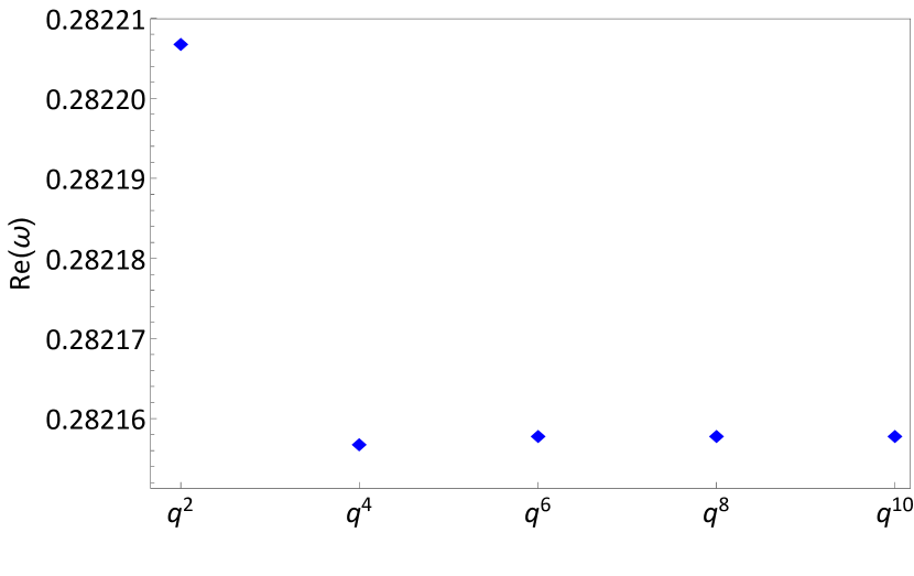
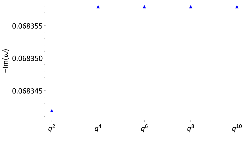
Figure 1: QNMs of axial gravitational perturbation for varying the expanding order of $q$, here we set $l=2$, $n=0$, $q=0.2$ and $\Lambda=0.05$.

Fig. 2 and Fig. 3 show the QNMs of the axial and the polar parts of the gravitational perturbation for $l=2$ and $n=0$, respectively. The figures reveal that, with the increase of $q$, the real part will increase but the imaginary part will increase first and then decrease. The specific data of QNM frequencies are place in Appendix C. The data in Table 2 indicate that there exist breaking of isospectrality of QNMs in Bardeen de Sitter BHs.

Note that one should confirm this breaking of isospectrality is not caused by the WKB approach method. We calculate the QNM by using various order of WKB approach, and find that the error caused by considering various order of WKB approach is much smaller than the breaking of isospectral when $q=0.6$. Therefore, we consider that the axial and the polar gravitational perturbations of Bardeen de Sitter BHs are not isospectral.

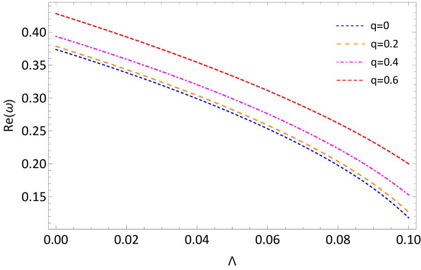
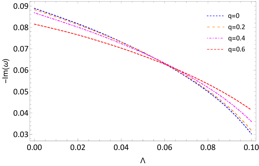
Figure 2: The QNM frequencies of the axial gravitational perturbation of the Bardeen de Sitter BHs for $l=2,n=0$.

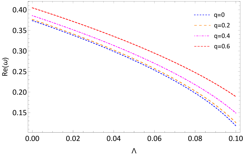
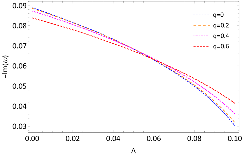
Figure 3: The QNM frequencies of the polar gravitational perturbation of the Bardeen de Sitter BHs for $l=2,n=0$.

In Fig. 4, we show the relative gap between the axial gravitational and the polar gravitational QNM frequencies, where $\Delta\omega$ is defined as

$$\Delta\omega=\frac{\omega^{\text{odd}}-\omega^{\text{even}}}{\omega^{\text{odd}}}\times 100{\%}.$$ (55)

This result clearly shows that with the increase of the charge $q$, isospectrality will be broken in Bardeen de Sitter spacetime.

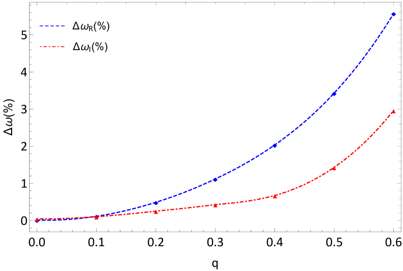
Figure 4: The relative gap between the axial and the polar QNMs of Bardeen de Sitter BHs with $\Lambda=0,q=0.6$ and $l=2,n=0$.

IV The Quasinormal Modes for Bardeen Anti-de Sitter Black Hole

IV.1 HH method

For Bardeen de Sitter BH, we use the HH method to calculate the QNMs HH ; Cardoso2001 . A brief introduction of this method is as follows. For axial sector, we write $\phi^{(-)}$ for a generic wavefunction as

$$\phi^{(-)}=e^{i\omega r_{*}}\psi^{(-)},$$ (56)

the Schrödinger-like equation becomes as

$$f(r)\frac{\partial^{2}{\phi^{(-)}}}{\partial{r}^{2}}+\left[f^{\prime}(r)-2i\omega\right]\frac{\partial\phi^{(-)}}{\partial r}-\frac{V}{f(r)}\phi^{(-)}=0.$$ (57)

And for the polar sector, from Eq. (47) we consider that $\phi^{(+)}$ can be written as

$$\phi^{(+)}=e^{i\omega z}Z$$ (58)

and satisfied

$$g(r)\frac{\partial^{2}{\phi^{(+)}}}{\partial{r}^{2}}+\left[g^{\prime}(r)-2i\omega\right]\frac{\partial\phi^{(+)}}{\partial r}-\frac{V}{g(r)}\phi^{(+)}=0$$ (59)

where

$$\frac{\partial r}{\partial z}=f(r)\sqrt{\frac{\sigma\tau}{rN}}=g(r)$$ (60)

Then introducing a transformation $x=1/r$ to restrict the studied region $r_{h}<r<\infty$ to a finite region $0<x<x_{h}$, expanding Eqs. (57) and (59) at the horizon $x_{h}$, we obtain

$$s(x)\frac{d^{2}}{dx^{2}}\phi(x)+\frac{t(x)}{x-x_{h}}\frac{d}{dx}\phi(x)+\frac{u(x)}{\left(x-x_{h}\right)^{2}}\phi(x)=0.$$ (61)

The coefficient functions $s(x)$, $t(x)$ and $u(x)$ can be expanded at horizon $x=x_{h}$,

$$s(x)=\sum_{n=0}^{\infty}s_{n}(x-x_{h})^{n}$$ (62)

and similarly for $t(x)$ and $u(x)$. Note that $u(x_{h})=0$ yields that $u_{0}=0$. After that, we consider the solution for Eqs. (57) and (59),

$$\phi(x)=\sum^{\infty}_{n=0}a_{n}(\omega)\left(x-x_{h}\right)^{n},$$ (63)

and Eq. (61) gives

$$a_{n}(\omega)=-\frac{1}{P_{n}}\sum_{k=0}^{n-1}\left[k(k-1)s_{n-k}+kt_{n-k}+u_{n-k}\right]a_{k},$$ (64)

where

$$P_{n}=n(n-1)s_{0}+nt_{0}.$$ (65)

Using the boundary condition $\phi=0$ at infinity, i.e., $x=0$,

$$\sum^{\infty}_{n=0}a_{n}(\omega)\left(-x_{h}\right)^{n}=0$$ (66)

Now the problem is reduced to that of finding a numerical solution of Eq. (66). Since one can not get a full sum from $0$ to infinity, the summation should be cut off at an appropriate position $N$. Taking a partial sum from $0$ to $N$, the numerical roots for $\omega_{N}$ of Eq. (66) can be evaluated by some numerical method. Then we move onto the case that taking a partial sum from $0$ to $N+1$, and similarly determine $\omega_{N+1}$. Comparing $\omega_{N}$ and $\omega_{N+1}$ can help us determine $N$ to achieve certain computational accuracy. It shows that when $N=50$ for axial perturbation or $N=150$ for polar perturbation, the calculation accuracy have 3 significant digits. Note that in Bardeen Anti-de Sitter spacetime, we set $\Lambda=-3$.

IV.2 Numerical Results of QNMs

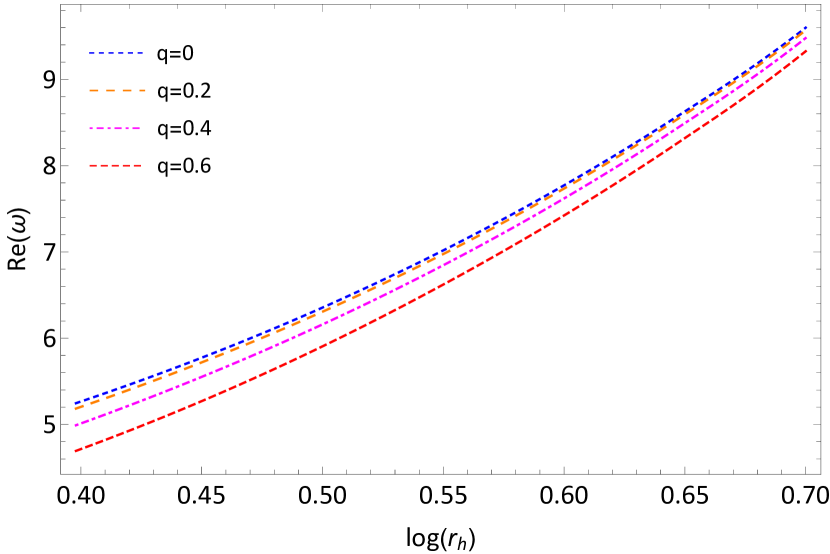
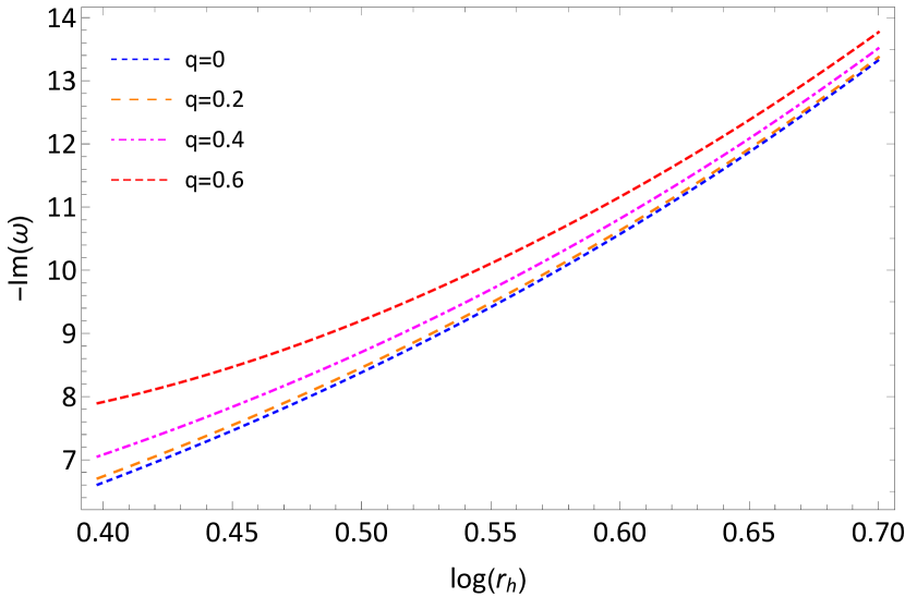
Figure 5: The QNM frequencies of the axial gravitational perturbation of the Bardeen Anti-de Sitter BHs with $l=2$ and $n=1$.

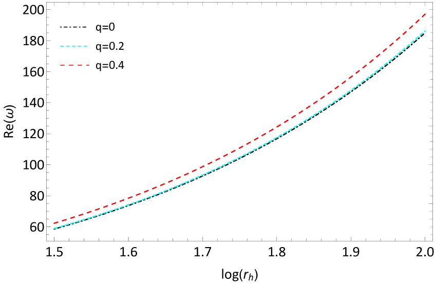
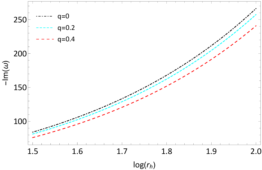
Figure 6: The QNM frequencies of the polar gravitational perturbation of the Bardeen Anti-de Sitter BHs with $l=2,n=0$.

Here we use HH method to calculate the QNMs of the Bardeen de Sitter BHs, and study the influence of magnetic charge $q$ on QNMs. The range of $r_{h}$ is limited to $r_{h}\in\left[1,100\right]$. The specific data are placed in Appendix C. Fig. 5 and Fig. 6 show the axial and the polar parts of the gravitational QNMs frequencies for Bardeen Anti-de Sitter spacetime. For the axial gravitational perturbation, we only consider the range $\log{r_{h}}\in[0.4,0.7]$, to obviously show that as the charge $q$ increase, the real part and the imaginary of $\omega$ will decrease. While for the polar gravitational perturbation, we only consider the range $\log{r_{h}}\in[1.5,2.0]$ where the deviations which due to the presence of charge $q$ can be clearly seen.

V Conclusion And Discussion

In this study, we investigate the gravitational perturbations of the Bardeen BH in the presence of a cosmological constant. Both the axial (odd-parity) and polar (even-parity) sectors are considered, we provide the detailed construction process for the decoupled equations with source terms. Then we derive Schrödinger-type equations with effective potentials given by equations (43) and (47). Subsequently, we apply the WKB approach to analyze the quasinormal modes (QNMs) for the Bardeen de Sitter spacetime. The obtained QNM frequencies are presented in Tables 1 and 2. We explore various combinations of values for $q$ and $\Lambda$ while fixing $l$ and $n$, and vice versa. The results reveal deviations between the QNM frequencies in the polar sector and those in the axial sector. To ensure that these deviations are not due to numerical errors, we conduct additional calculations using different orders of $q$ and the WKB approach. Our findings demonstrate a convergence behavior, suggesting that the deviations are not caused by the order of $q$ or the WKB approach (and the currently used orders are sufficiently high to ensure the required accuracy of our conclusions). Moreover, numerical analysis indicates that the errors arising from different choices of the orders of $q$ and the WKB approach are significantly smaller than the observed deviations. This provides evidence that the deviations are caused by the inherent differences in odd and even parities, rather than the order of $q$ or the WKB approach.

The results unequivocally demonstrate that, for a fixed nonlinear electromagnetic charge $q$, the axial and polar gravitational perturbations exhibit distinct QNM frequencies. This observation indicates a violation of isospectrality in the case of Bardeen de Sitter BHs. Unlike linear electromagnetic fields, the presence of nonlinear electromagnetic fields disrupts the isospectrality of gravitational perturbations.

Furthermore, we also compute the QNMs of the Bardeen Anti-de Sitter spacetime. To gain a clearer understanding of the impact of varying $q$ on the QNMs, we consider different ranges for the parameter $r_{h}$. Our results show the influence of the parameter $q$ on the real and imaginary parts of the QNMs.

It is worth noting that the master equations derived in this paper contain source terms. In this paper, due to calculation the QNMs, we impose the source terms vanish. However, if we consider the extreme mass ratio inspiral model, i.e., a point particle moving around the Bardeen BH, using our master equations one can calculate the energy flux at infinity or the gravitational wave of inspiral phase. On the other hand, the Bardeen BH considered in this paper is a simple RBH solution. The ABG solution seems to be a more reasonable choice as it approaches the Reissner-Nordström solution at asymptotic infinity EAAG1 . Whether the breaking of isospectrality occurs in all nonlinear electromagnetic theories is worth further exploration. With the improvement of detection sensitivity, in the near future, LIGO/Virgo/KAGRA cooperation is expected to accurately measure the QNMs of the BH ringdown phase and confirm/deny the breaking of isospectrality from the QNM signal.

Appendix A Explicit Expressions for $E_{\mathrm{A}}$-$E_{\mathrm{K}}$

By projecting the perturbed metric $h^{lm}_{ab}$ onto these orthogonal tensor base bases, the expressions for coefficients A-K can be obtained.

$$\mathrm{A} = f^{2}\oint h^{lm}_{ab}(v^{a}v^{b}Y^{\ast}_{lm})d\Omega,$$

$$\mathrm{B} = -\frac{f}{l(l+1)}\oint h^{lm}_{ab}v^{a}Y^{b\ast}_{E,lm}d\Omega,$$

$$\mathrm{C} = -\frac{f}{l(l+1)}\oint h^{lm}_{ab}v^{a}Y^{b\ast}_{B,lm}d\Omega,$$

$$\mathrm{D} = -\oint h^{lm}_{ab}v^{a}Y^{b\ast}_{R,lm}d\Omega,$$

$$\mathrm{E} = \frac{1}{2}\oint h_{ab}^{lm}T^{ab\ast}_{T0,lm}d\Omega,$$

$$\mathrm{F} = \frac{2(l-2)!}{(l+2)!}\oint h_{ab}^{lm}T^{ab\ast}_{E2,lm}d\Omega,$$

$$\mathrm{G} = \frac{2(l-2)!}{(l+2)!}\oint h_{ab}^{lm}T^{ab\ast}_{B2,lm}d\Omega,$$

$$\mathrm{H} = \frac{1}{l(l+1)f}\oint h^{lm}_{ab}T^{ab\ast}_{E1,lm}d\Omega,$$

$$\mathrm{J} = \frac{1}{l(l+1)f}\oint h^{lm}_{ab}T^{ab\ast}_{B1,lm}d\Omega,$$

$$\mathrm{K} = \frac{1}{f^{2}}\oint h^{lm}_{ab}T^{ab\ast}_{L0,lm}d\Omega.$$ (67)

Only the case of $l\geq 2$ is considered in this paper.

Fild equation of ${E}_{A}-{E}_{K}$

$$E_{\mathrm{A}}= - \frac{2(f-1+r^{2}\Lambda+2r^{2}\mathcal{L}+rf^{\prime})}{r^{2}}\mathrm{A}$$ (68)

$$- \frac{(l^{2}+l+2f+4rf^{\prime})f^{2}}{r^{2}}\mathrm{K}-\frac{2f^{3}}{r}\frac{\partial}{\partial r}\mathrm{K}$$

$$- \frac{(l^{2}+l-2)f}{r^{2}}\mathrm{E}+\frac{f(6f+rf^{\prime})}{r}\frac{\partial}{\partial r}\mathrm{E}+2f^{2}\frac{\partial^{2}}{\partial r^{2}}\mathrm{E}~{}~{}~{}~{}$$

$$E_{\mathrm{B}}=-\frac{f^{\prime}}{r}\mathrm{D}-\frac{f}{r}\frac{\partial}{\partial r}\mathrm{D}-\frac{1}{r}\frac{\partial}{\partial t}\mathrm{E}-\frac{f}{r}\frac{\partial}{\partial t}\mathrm{K},~{}~{}~{}~{}~{}~{}~{}~{}~{}~{}~{}~{}~{}~{}~{}~{}~{}~{}~{}~{}~{}~{}~{}~{}$$ (69)

$$E_{\mathrm{C}}= - \frac{l^{2}+l-2+2r^{2}\Lambda+2f+2rf^{\prime}+r^{2}f^{\prime\prime}+4r^{2}\mathcal{L}}{r^{2}}\mathrm{C}$$ (70)

$$+ \frac{2f}{r}\frac{\partial}{\partial r}\mathrm{C}+f\frac{\partial^{2}}{\partial r^{2}}\mathrm{C}+\frac{3f}{r}\frac{\partial}{\partial t}\mathrm{J}+f\frac{\partial^{2}}{\partial t\partial r}\mathrm{J},~{}~{}~{}~{}~{}~{}$$

$$E_{\mathrm{D}}= - \frac{l^{2}+l-2+2r^{2}\Lambda+2f+4r^{2}\mathcal{L}+2rf^{\prime}}{r^{2}}\mathrm{D}$$ (71)

$$+ \frac{rf^{\prime}-2f}{rf}\frac{\partial}{\partial t}\mathrm{E}-2\frac{\partial^{2}}{\partial t\partial r}\mathrm{E}+\frac{2f}{r}\frac{\partial}{\partial t}\mathrm{K},~{}~{}~{}~{}~{}~{}~{}~{}~{}~{}~{}~{}~{}~{}~{}~{}~{}~{}~{}$$

$$E_{\mathrm{E}}= - \frac{f(l^{2}+l+2rf^{\prime}+2r^{2}f^{\prime\prime})-r^{2}{f^{\prime}}^{2}}{2r^{2}f^{2}}\mathrm{A}-\frac{rf^{\prime}-2f}{2rf}\frac{\partial}{\partial r}\mathrm{A}$$ (72)

$$+ \frac{\partial^{2}}{\partial r^{2}}\mathrm{A}+\frac{2f+rf^{\prime}}{rf}\frac{\partial}{\partial t}\mathrm{D}+2\frac{\partial^{2}}{\partial t\partial r}\mathrm{D}$$

$$- \frac{4r\mathcal{L}+2f^{\prime}+r(2\Lambda+2r\mathcal{L}^{\prime}+f^{\prime\prime})}{r}\mathrm{E}$$

$$+ \frac{r^{3}\mathcal{L}^{\prime}-2f-rf^{\prime}}{r}\frac{\partial}{\partial r}\mathrm{E}-f\frac{\partial^{2}}{\partial r^{2}}\mathrm{E}+\frac{1}{f}\frac{\partial^{2}}{\partial t^{2}}\mathrm{E}$$

$$+ \frac{r^{2}{f^{\prime}}^{2}+f(l^{2}+l+6rf^{\prime}+2r^{2}f^{\prime\prime})}{2r^{2}}\mathrm{K}$$

$$+ \frac{f(2f+rf^{\prime})}{2r}\frac{\partial}{\partial r}\mathrm{K}+\frac{\partial^{2}}{\partial t^{2}}\mathrm{K},$$

$$E_{\mathrm{F}} = -\frac{1}{r^{2}f}\mathrm{A}+\frac{f}{r^{2}}\mathrm{K},~{}~{}~{}~{}~{}~{}~{}~{}~{}~{}~{}~{}~{}~{}~{}~{}~{}~{}~{}~{}~{}~{}~{}~{}~{}~{}~{}~{}~{}~{}~{}~{}~{}~{}~{}~{}~{}~{}~{}~{}~{}~{}~{}~{}~{}~{}~{}~{}~{}~{}~{}~{}~{}~{}~{}~{}~{}~{}~{}~{}$$ (73)

$$E_{\mathrm{G}}=-\frac{2}{rf}\frac{\partial}{\partial t}\mathrm{C}-\frac{2f+2rf^{\prime}}{r^{2}}\mathrm{J}-\frac{2f}{r}\frac{\partial}{\partial r}\mathrm{J},~{}~{}~{}~{}~{}~{}~{}~{}~{}~{}~{}~{}~{}~{}~{}~{}~{}~{}~{}~{}~{}~{}~{}~{}~{}~{}~{}~{}~{}~{}~{}$$ (74)

$$E_{\mathrm{H}} =\frac{2f+rf^{\prime}}{2r^{2}f^{2}}\mathrm{A}-\frac{1}{rf}\frac{\partial}{\partial r}\mathrm{A}-\frac{1}{rf}\frac{\partial}{\partial t}\mathrm{D}+\frac{1}{r}\frac{\partial}{\partial r}\mathrm{E}$$

$$~{}~{}~{}~{}~{}-\frac{2f+rf^{\prime}}{2r^{2}}\mathrm{K},~{}~{}~{}~{}~{}~{}~{}~{}~{}~{}~{}~{}~{}~{}~{}~{}~{}~{}~{}~{}~{}~{}~{}~{}~{}~{}~{}~{}~{}~{}~{}~{}~{}~{}~{}~{}~{}~{}~{}~{}~{}~{}~{}~{}~{}~{}~{}~{}~{}~{}~{}~{}~{}~{}~{}~{}~{}~{}~{}~{}~{}~{}~{}$$ (75)

$$E_{\mathrm{J}} =\frac{1}{rf}\frac{\partial}{\partial t}\mathrm{C}-\frac{1}{f}\frac{\partial^{2}}{\partial t\partial r}\mathrm{C}-\frac{1}{f}\frac{\partial^{2}}{\partial t^{2}}\mathrm{J}$$

$$~{}~{}~{}~{}~{}-\frac{l^{2}+l-2+2r^{2}\Lambda+4r^{2}\mathcal{L}+2rf^{\prime}+r^{2}f^{\prime\prime}}{r^{2}}\mathrm{J},~{}~{}~{}~{}$$ (76)

$$E_{\mathrm{K}}= - \frac{l^{2}+l+2rf^{\prime}}{r^{2}f^{2}}\mathrm{A}+\frac{2}{rf}\frac{\partial}{\partial r}\mathrm{A}+\frac{4}{rf}\frac{\partial}{\partial t}\mathrm{D}+\frac{l^{2}+l-2}{r^{2}f}E$$ (77)

$$- \frac{2f+rf^{\prime}}{rf}\frac{\partial}{\partial r}\mathrm{E}+\frac{2}{f^{2}}\frac{\partial^{2}}{\partial t^{2}}\mathrm{E}$$

$$- \frac{2(2r^{2}\mathcal{L}-1+r^{2}\Lambda)}{r^{2}}\mathrm{K},~{}~{}~{}~{}~{}~{}~{}~{}~{}~{}~{}~{}~{}~{}~{}~{}~{}~{}~{}~{}~{}~{}~{}~{}~{}~{}~{}~{}~{}~{}~{}~{}~{}~{}~{}~{}~{}~{}~{}~{}~{}~{}~{}~{}~{}~{}~{}$$

Appendix B Expressions For Parameters in Eqs. (41) and (II)

Here we present the explicit expressions of the parameters in Eq. (41), which are given by

$$N= -4f^{2}\mu-\sigma\left(-\rho\sigma+2f^{\prime}\right)+2f\left(\gamma\sigma-\nu\sigma+\sigma^{\prime}\right),$$ (78)

$$\sigma= -2+\lambda+2r^{2}\Lambda+2f+2rf^{\prime}+4r^{2}\kappa\mathcal{L},$$ (79)

$$\tau= -2+\lambda+2r^{2}\Lambda+3rf^{\prime}+4r^{2}\kappa\mathcal{L},$$ (80)

$$c_{0}= \frac{1}{2fN\sigma^{2}}\bigg{\{}-2f^{2}M_{1}N\mu-M_{1}N\sigma f^{\prime}$$

$$+f\Big{[}\sigma NM_{1}^{\prime}-\sigma M_{1}N^{\prime}+M_{2}N\left(-\nu\sigma+\sigma^{\prime}\right)\Big{]}\bigg{\}},$$ (81)

$$c_{1}= \frac{1}{2N\sigma}\bigg{\{}M_{1}N-f\Big{[}N^{2}+2f\sigma N^{\prime}$$

$$+2N\left(2f^{2}\mu+f\nu\sigma-\sigma f^{\prime}-2f\sigma^{\prime}\right)\Big{]}\bigg{\}},$$ (82)

and the parameters appearing in the source term Eq. (II) are given by

$$M_{F}= \frac{r}{\tau}\left(\eta+\lambda\sigma-2f\sigma+rf^{\prime}\sigma\right),$$ (83)

$$N_{A}= \frac{1}{4f^{2}N\sigma^{2}}\bigg{\{}rN^{2}+2rf\sigma N^{\prime}$$

$$+2N\Big{[}2rf^{2}\mu+2r\sigma f^{\prime}+f\left(-\sigma+r\nu\sigma-r\sigma^{\prime}\right)\Big{]}\bigg{\}},$$ (84)

$$N_{F}= \frac{1}{4fN\sigma^{2}\tau}\bigg{\{}rN^{2}\eta+2fM_{F}\sigma\tau N^{\prime}+2N\tau\Big{[}2f^{2}M_{F}\mu$$

$$+M_{F}\sigma f^{\prime}-f\left(\sigma M_{F}^{\prime}-\nu\sigma M_{F}+\sigma^{\prime}M_{F}\right)\Big{]}\bigg{\}},$$ (85)

Here we have,

$$M_{1}= f\Big{[}\rho\sigma^{2}+f\left(-2\nu\sigma+2\sigma^{\prime}\right)\Big{]},$$ (86)

$$M_{2}= 2f\left(2f^{2}\mu-f\gamma\sigma+\sigma f^{\prime}\right),$$ (87)

$$\eta= 4-\lambda^{2}-8r^{2}\Lambda+4r^{4}\Lambda^{2}+4f^{2}+16r^{4}\kappa^{2}\mathcal{L}^{2}$$

$$-8rf^{\prime}-rf^{\prime}\lambda+8r^{3}f^{\prime}\Lambda+4r^{2}f^{\prime 2}$$

$$+16r^{2}\kappa\mathcal{L}\left(r^{2}\Lambda+rf^{\prime}-1\right)$$

$$+2f\left(-4+\lambda+4r^{2}\Lambda+8r^{2}\kappa\mathcal{L}+4rf^{\prime}\right),$$ (88)

$$\gamma= -\frac{1}{2f\left(\lambda-2+2r^{2}\Lambda+4r^{2}\kappa\mathcal{L}+3rf^{\prime}\right)}$$

$$\bigg{\{}4f\left(r\Lambda+2r\kappa\mathcal{L}+f^{\prime}\right)$$

$$+f^{\prime}\left(\lambda-2+2r^{2}\Lambda+4r^{2}\kappa\mathcal{L}+4rf^{\prime}\right)\bigg{\}},$$ (89)

$$\rho= \frac{1}{r}-\frac{f^{\prime}}{\lambda-2+2r^{2}\Lambda+4r^{2}\kappa\mathcal{L}+3rf^{\prime}},$$ (90)

$$\nu= -\frac{1}{2rf\left(\lambda-2+2r^{2}\Lambda+4r^{2}\kappa\mathcal{L}+3rf^{\prime}\right)}\times$$

$$\bigg{\{}2f\left(\lambda-2+2r^{2}\Lambda+4r^{2}\kappa\mathcal{L}+4rf^{\prime}\right)+$$

$$rf^{\prime}\Big{[}-rf^{\prime}+5\left(\lambda-2+2r^{2}\Lambda+4r^{2}\kappa\mathcal{L}+3rf^{\prime}\right)\Big{]}\bigg{\}},$$ (91)

$$\mu= \frac{1}{4rf^{2}\left(\lambda-2+2r^{2}\Lambda+4r^{2}\kappa\mathcal{L}+3rf^{\prime}\right)}\times$$

$$\bigg{\{}8f^{2}\left(\lambda-2+r^{2}\Lambda+2r^{2}\kappa\mathcal{L}+2rf^{\prime}\right)$$

$$-r^{2}f^{\prime 2}\left(\lambda-2+2r^{2}\Lambda+4r^{2}\kappa\mathcal{L}+2rf^{\prime}\right)$$

$$+2f\Big{[}r^{2}f^{\prime 2}+rf^{\prime}\left(-12+6\lambda+2r^{2}\Lambda-3r^{2}f^{\prime\prime}\right)$$

$$+\left(\lambda-2+2r^{2}\Lambda\right)\left(2\lambda-4-r^{2}f^{\prime\prime}\right)$$

$$-4r^{2}\kappa\mathcal{L}\left(4-2\lambda-rf^{\prime}+r^{2}f^{\prime\prime}\right)\Big{]}\bigg{\}}.$$ (92)

Appendix C Quasinormal Modes Frequencies

Table 1: QNM frequencies of the gravitational perturbations calculated by WKB approach with different $l$ and $n$ in Badeen de Sitter spacetime, the parameters are chosen as $q=0.1$ and $\Lambda=0.02$.

$l$	$n$	odd parity		even parity		relative deviation
		Re($\omega$)	-Im($\omega$)	Re($\omega$)	-Im($\omega$)	Re($\omega$)	-Im($\omega$)
2	0	0.3396	0.0816	0.3392	0.0817	0.1178%	0.1225%
	1	0.3201	0.2485	0.3196	0.2490	0.1562%	0.2012%
3	0	0.5446	0.0844	0.5443	0.0844	0.0551%	0%
	1	0.5323	0.2551	0.5320	0.2552	0.0564%	0.0392%
	2	0.5087	0.4316	0.5083	0.4316	0.0786%	0%
4	0	0.7348	0.0855	0.7346	0.0855	0.0272%	0%
	1	0.7256	0.2577	0.7253	0.2577	0.0413%	0%
	2	0.7076	0.4331	0.7073	0.4331	0.0424%	0 %
	3	0.6818	0.6142	0.6816	0.6142	0.0293%	0 %
5	0	0.9190	0.0861	0.9188	0.0861	0.0218%	0%
	1	0.9116	0.2589	0.9114	0.2589	0.0219%	0%
	2	0.8970	0.4339	0.8968	0.4339	0.0223%	0 %
	3	0.8758	0.6126	0.8756	0.6126	0.0228%	0 %
	4	0.8488	0.7964	0.8485	0.7964	0.0353%	0 %

Table 2: QNM frequencies of the gravitational perturbations calculated by WKB approach with different $q$ and $\Lambda$ in Badeen de Sitter spacetime, here $l=2$ and $n=0$.

$q$	$\Lambda$	odd parity		even parity		relative deviation
		Re($\omega$)	-Im($\omega$)	Re($\omega$)	-Im($\omega$)	Re($\omega$)	-Im($\omega$)
0.2	0.00	0.3784	0.0883	0.3766	0.0886	0.4757%	0.3238%
	0.02	0.3432	0.0813	0.3415	0.0815	0.4953%	0.2472%
	0.04	0.3039	0.0731	0.3023	0.0732	0.5265%	0.1752%
	0.06	0.2586	0.0631	0.2572	0.0632	0.5414%	0.1220%
	0.08	0.2035	0.0504	0.2024	0.0505	0.5405%	0.1646%
	0.10	0.1265	0.0318	0.1258	0.0318	0.5534%	0%
0.4	0.00	0.3935	0.0868	0.3859	0.0873	1.9314%	0.5760%
	0.02	0.3588	0.0801	0.3515	0.0800	2.0346%	0.1248%
	0.04	0.3202	0.0724	0.3134	0.0728	2.1237%	0.5525%
	0.06	0.2760	0.0633	0.2699	0.0636	2.2101%	0.4739%
	0.08	0.2230	0.0519	0.2179	0.0520	2.2870%	0.1927%
	0.10	0.1527	0.0360	0.1491	0.0361	2.3576%	0.2778%
0.6	0.00	0.4282	0.0815	0.4049	0.0839	5.4414%	2.9448%
	0.02	0.3927	0.0765	0.3718	0.0780	5.3221%	1.9608%
	0.04	0.3542	0.0703	0.3355	0.0711	5.2795%	1.1380%
	0.06	0.3113	0.0628	0.2947	0.0632	5.3325%	0.6369%
	0.08	0.2616	0.0535	0.2475	0.0537	5.3899%	0.3738%
	0.10	0.1999	0.0414	0.1890	0.0414	5.4527%	0%

Table 3: The axial gravitational QNM frequencies of the Bardeen Anti-de Sitter spacetime calculated by the HH method with different $q$ and $r_{h}$, where the cosmological constant is set as $\Lambda=-3$, and the cut off number of the summation is determined as $N=50$.

$q$	$r_{h}$	$l=2,n=0$		$l=2,n=1$		$l=3,n=0$		$l=3,n=1$
		Re($\omega$)	-Im($\omega$)	Re($\omega$)	-Im($\omega$)	Re($\omega$)	-Im($\omega$)	Re($\omega$)	-Im($\omega$)
0.2	2	0~	0.816839	4.36465	5.38995	0~	2.38847	4.47733	5.22429
	4	0~	0.369257	7.76816	10.6822	0~	0.913702	7.93976	10.6235
	6	0~	0.242054	11.3485	16.0005	0~	0.587737	11.4762	15.9616
	8	0~	0.180492	14.9857	21.3237	0~	0.435592	15.0850	21.2945
	10	0~	0.144009	18.6470	26.6488	0~	0.346595	18.7277	26.6254
	50	0~	0.028672	92.5018	133.195	0~	0.068692	92.5184	133.190
	100	0~	0.014334	184.957	266.386	0~	0.034337	184.966	266.384
0.4	2	0~	1.10090	4.10727	5.91645	0~	3.29842	3.88143	6.03826
	4	0~	0.455923	7.65404	10.8665	0~	1.01260	7.82060	10.8118
	6	0~	0.295336	11.2736	16.1174	0~	0.643960	11.4004	16.0793
	8	0~	0.219352	14.9298	21.4100	0~	0.475610	15.0288	21.3810
	10	0~	0.174700	18.6023	26.7173	0~	0.377861	18.6829	26.6940
	50	0~	0.034677	92.4929	133.208	0~	0.074702	92.5095	133.204
	100	0~	0.017335	184.953	266.393	0~	0.037338	184.961	266.391
0.6	2	0~	1.64729	4.34131	7.41637	0~	~	5.19887	7.46867
	4	0~	0.601735	7.45796	11.2095	0~	1.18029	7.61522	11.1654
	6	0~	0.384439	11.1468	16.3213	0~	0.738091	11.2720	16.2847
	8	0~	0.284234	14.8357	21.5573	0~	0.542447	14.9342	21.5289
	10	0~	0.225908	18.5275	26.8332	0~	0.430034	18.6079	26.8102
	50	0~	0.044687	92.4781	133.231	0~	0.084719	92.4947	133.226
	100	0~	0.022336	184.946	266.404	0~	0.042340	184.954	266.402

Table 4: The polar gravitational QNM frequencies of the Bardeen Anti-de Sitter spacetime calculated by the HH method with different $q$ and $r_{h}$, where the cosmological constant is set as $\Lambda=-3$, and the cut off number of the summation is determined as $N=150$.

$q$	$r_{h}$	$l=2,~{}n=0$		$l=3,~{}n=0$
		Re($\omega$)	-Im($\omega$)	Re($\omega$)	-Im($\omega$)
0.2	2	4.48199	3.95046	4.58341	3.30879
	4	8.03115	9.55387	8.32398	8.57327
	6	11.5906	14.9412	11.9309	14.3709
	8	15.2177	20.2144	15.4865	19.9298
	10	18.8806	25.4391	19.0817	25.3612
	50	93.1610	128.669	92.8456	130.662
	100	186.243	257.431	185.524	261.567
0.4	2	4.39016	3.82357	4.53669	3.32935
	4	8.20505	8.94905	8.20260	8.38047
	6	12.0580	13.9709	11.8863	13.8573
	8	15.9442	18.9028	15.5437	19.1484
	10	19.8492	23.7920	19.2304	24.3338
	50	98.5247	120.387	94.3123	125.134
	100	197.003	240.864	188.5045	250.488

References

• (1) B. P. Abbott et al. [LIGO Scientific and Virgo Collaborations], Observation of gravitational waves from a binary black hole merger, Phys. Rev. Lett. 116, 061102 (2016).
• (2) K. Akiyama et al. [Event Horizon Telescope Collaborations], First M87 event horizon telescope results, Astrophys. J. Lett. 875 L1, L2, L3, L4, L5, L6 (2019).
• (3) K. Akiyama et al. [Event Horizon Telescope Collaborations], First Sagittarius $A^{\ast}$ Event Horizon Telescope results, Astrophys. J. Lett. 930 L12, L13, L14, L15, L16, L17 (2022).
• (4) C. Lan, H. Yang, Y. Guo and Y. Miao, Regular black holes: A short topic review, arXiv: 2303.11696
• (5) J. Bardeen, Non-singular general-relativistic gravitational collapse, Proceedings of GR5, Tiflis, U.S.S.R. (1968).
• (6) E. Ayón-Beato and A. García, Regular black hole in general relativity coupled to nonlinear electrodynamics, Phys. Rev. Lett. 80, 5056 (1998).
• (7) E. Ayón-Beato and A. García, New regular black hole solution from nonlinear electrodynamics, Phys. Lett. B 464, 25 (1999).
• (8) E. Ayón-Beato and A. García, The Bardeen model as a nonlinear magnetic monopole, Phys. Lett. B 493, 149 (2000).
• (9) K. A. Bronnikov, Regular magnetic black holes and monopoles from nonlinear electrodynamics, Phys. Rev. D 63, 044005 (2001).
• (10) S. A. Hayward, Formation and evaporation of nonsingular black holes, Phys. Rev. Lett. 96, 031103 (2006).
• (11) M. Cataldo and A. García, Regular (2+1)-dimensional black holes within nonlinear electrodynamics, Phys. Rev. D 61, 084003 (2000).
• (12) K. A. Bronnikov and J. C. Fabris, Regular phantom black holes, Phys. Rev. Lett. 96, 251101 (2006).
• (13) S. G. Ghosh and S. D. Maharaj, Radiating Kerr-like regular black hole, Eur. Phys. J. C 75: 1-9 (2015).
• (14) A. Burinskii and S. R. Hildebrandt, New type of regular black holes and particlelike solutions from nonlinear electrodynamics, Phys. Rev. D 65, 104017 (2002).
• (15) T. Regge and J. A. Wheeler, Stability of a Schwarzschild singularity, Phys. Rev. 108, 1063 (1957).
• (16) F. J. Zerilli, Effective potential for even parity Regge-Wheeler gravitational perturbation equations, Phys. Rev. Lett. 24, 737 (1970).
• (17) F. J. Zerilli, Gravitational field of a particle falling in a Schwarzschild geometry analyzed in tensor harmonics, Phys. Rev. D 2, 2141 (1970).
• (18) S. Chandrasekhar, The mathematical theory of black holes (Oxford University Press, Inc. New York, 1992).
• (19) J. S. F. Chan and R. B. Mann, Scalar wave falloff in asymptotically Anti-de Sitter backgrounds, Phys. Rev. D 55, 7546 (1997).
• (20) G. T. Horowitz and V. E. Hubeny, Quasinormal modes of AdS black holes and the approach to thermal equilibrium, Phys. Rev. D 62, 024027 (2000).
• (21) V. Cardoso and J. P. S. Lemos, Quasinormal modes of Schwar-zschild anti de Sitter black holes: Electromagnetic and gravitational perturbations, Phys. Rev. D 64, 084017 (2001).
• (22) S. Hod, Bohr’s correspondence principle and the area spectrum of quantum black holes, Phys. Rev. Lett. 81, 4293 (1998).
• (23) M. Maggiore, Physical interpretation of the spectrum of black hole quasinormal modes, Phys. Rev. Lett. 100, 141301 (2008).
• (24) S. Fernando and J. Correa, Quasinormal modes of the Bardeen black hole: scalar perturbations, Phys. Rev. D 86, 64039 (2012).
• (25) A. Flachi and J. P. S. Lemos, Quasinormal modes of regular black holes, Phys. Rev. D 87, 024034 (2013).
• (26) S. C. Ulhoa, On quasinormal modes for gravitational perturbations of Bardeen black hole, Braz. Jour. Phys. 44, 380 (2014).
• (27) C. Moreno and O. Sarbach, Stability properties of black holes in self-gravitatting non-linear electrodynamics, Phys. Rev. D 67, 024028 (2003).
• (28) E. Chaverra, J. C. Degollado, C. Moreno and O. Sarbach, Black holes in nonlinear electrodynamics: Quasinormal spectra and parity splitting, Phys. Rev. D 93, 123013 (2016).
• (29) B. Toshmatov, Z. Stuchlík, J. Schee and B. Ahmedov, Electromagnetic perturbations of black holes in general relativity coupled to nonlinear electrodynamics, Phys. Rev. D 97, 084058 (2018).
• (30) B. Toshmatov, Z. Stuchlík and B. Ahmedov, Electromagnetic perturbations of black holes in general relativity coupled to nonlinear electrodynamics: Polar perturbations, Phys. Rev. D 98, 085021 (2018).
• (31) J. Li, H. Ma and K. Lin, Dirac quasinormal modes in spherically symmetric regular black holes, Phys. Rev. D 88, 064001 (2013).
• (32) S. Fernando, Bardeen-de Sitter black holes, Int. J. Mod. Phys. D 26, 1750071 (2017).
• (33) J. E. Thompson, H. Chen and B. F. Whiting, Gauge invariant perturbations of the Schwarzschild spacetime, Class. Quantum Grav. 34, 174001 (2017).
• (34) K. S. Thorne, Multipole expansions of gravitational radiation, Rev. Mod. Phys. 52, 299 (1980).
• (35) W. Liu, X. Fang, J. Jing and A. Wang, Gauge invariant perturbations of general spherically symmetric spacetimes, Sci. China, Phys. Mech. Astron. 66, 210411 (2023).
• (36) C. Zhang, T. Zhu, X. Fang and A. Wang, Imprints of dark matter on gravitational ringing of supermassive black holes, Physics of the Dark Universe. 37, 101078 (2022).
• (37) B. F. Schutz and C. M. Will, Black hole normal modes: A semianalytic approach, Astrophys. J. Lett. 291: L33-L36 (1985).
• (38) S. Iyer and C. M. Will, Black-hole normal modes: A WKB approach. I. Foundations and application of a higher-order WKB approach analysis of potential-barrier scattering, Phys. Rev. D 35, 3621 (1987).
• (39) S. Iyer, Black-hole normal modes: A WKB approach. II. Sch-warzschild black holes, Phys. Rev. D 35, 3632 (1987).
• (40) R. A. Konoplya, Quasinormal behavior of the D-dimensional Schwarzschild black hole and the higher order WKB approach, Phys. Rev. D 68, 024018 (2003).
• (41) J. Matyjasek and M. Opala, Quasinormal modes of black holes. The improved semianalytic approach, Phys. Rev. D 96, 024011 (2017).