Random Feedback Alignment Algorithms to train Neural Networks: Why do they Align?

Abstract

Feedback alignment algorithms are an alternative to backpropagation to train neural networks, whereby some of the partial derivatives that are required to compute the gradient are replaced by random terms. This essentially transforms the update rule into a random walk in weight space. Surprisingly, learning still works with those algorithms, including training of deep neural networks. This is generally attributed to an alignment of the update of the random walker with the true gradient — the eponymous gradient alignment — which drives an approximate gradient descend. The mechanism that leads to this alignment remains unclear, however. In this paper, we use mathematical reasoning and simulations to investigate gradient alignment. We observe that the feedback alignment update rule has fixed points, which correspond to extrema of the loss function. We show that gradient alignment is a stability criterion for those fixed points. It is only a necessary criterion for algorithm performance. Experimentally, we demonstrate that high levels of gradient alignment can lead to poor algorithm performance and that the alignment is not always driving the gradient descend.

1 Introduction

The backpropagation algorithm (BP) [1] underpins a good part of modern neural network (NN) based AI. BP-based training algorithms continue to be the state of the art in many areas of machine learning ranging from benchmark problems such as the MNIST dataset[2] to the most recent transformer-based architectures [3]. While its success is undeniable, BP has some disadvantages. The main one is that BP is computationally expensive. It is so in two ways. Firstly, BP has high requirements on pure processing power. It also requires sequential processing of layers during both the forward and backward pass, limiting its scope for parallelisation. This is sometimes called backward locking [4].

Secondly, BP is biologically implausible. One issue is that for every neuronal feedforward connection, BP would require neurons to also have a symmetric feedback connection with the same weight. This has never been observed. From a purely machine learning point of view, the lack of biological plausibility may not be too concerning, since the aim of applied AI is more often performance, rather than neuroscientific realism. However, there is a sense in which biological plausibility becomes a real concern after all: The update of any particular connection weight in a neural network requires global information about the entire network. This entails intense data processing needs [5], which in turn leads to high energy consumption [6, 7]. The electricity consumption required for the training of large scale NNs is a barrier to adoption and environmentally unsustainable and is widely recognised as problematic [8, 9]. BP is also not compatible with neuromorphic hardware platforms [10], such as Loihi [11] or SpiNNaker [12].

In the light of this, there has been some recent interest in alternatives to BP that alleviate these issues [13]. One particularly intriguing example are random feedback alignment (FA) algorithms [14]. The basic FA algorithm is just BP with the symmetric feedback weights replaced by a randomly chosen, but fixed, feedback matrix. A variant of FA is direct feedback alignment (DFA) [15], which bypasses backpropagation through layers and transmits the error directly to weights from the output layer via appropriately chosen feedback matrices. This enables layer-wise parallel updates of NNs. Furthermore, training no longer requires global knowledge of the entire network, which makes it amenable to implementation on neuromorphic hardware. FA and DFA have been found to perform surprisingly well on a number of benchmark problems [16, 17]. Recently, it has been reported that they even work on large-scale architectures such as transformers [18], often reaching performances that are comparable, albeit not exceeding, those of BP-based algorithms. Both algorithms do not work well on convolutional neural networks [18].

FA algorithms replace partial derivatives in the gradient computation by random matrices. Mathematically, the resulting update will no longer be a gradient of the loss function, but must be expected to be orthogonal to the gradient. It is therefore, at a first glance, surprising that DFA and FA work at all. A key insight into why they work was already given in the original paper by Lillicrap [14] who showed that the update direction of FA is not orthogonal to the gradient after all. They observed so-called weight alignment, whereby the weights of the network align with (i.e. point into approximately the same direction as) the feedback matrices and gradient alignment where the updates of the FA algorithm align with the gradient as computed by BP. They conjectured that this alignment drives the approximate gradient descent of FA.

A mechanism that could lead to this alignment was suggested by Refinetti and co-workers [19]. They modelled a linear two-layer network using a student-teacher setup based on an approach by Saad and Solla [20]. This showed that, at least in their setup, when starting from initially zero weights, the weight update is in the direction of the feedback matrix, leading to weight alignment and consequently gradient alignment. A corollary of their results is the prediction that alignment is particularly strong when the weights are initially vanishing. Another important theoretical contribution is by Nøkland [15] who formulated a stability criterion for DFA.

The above results were obtained using mathematically rigorous methods, but also rely on restrictive simplifying assumptions (e.g. linear networks in a student-teacher setup), which may or may not be relevant for realistic NNs. There is therefore a need to understand how FA operates in unrestricted NN, and whether the insights derived from simplified setups remain valid. The aim of the present contribution is to shed more light onto why FA works. To do this, we will complement existing approaches and view FA as a random walk [21], or more specifically a spatially inhomogeneous random walk in continuous weight space where the distribution of jump lengths and directions varies according to the position of the walker. In the present case, the update is entirely determined by the FA update rule and the distribution of training examples. The latter acts as the source of randomness.

We will show below that across weight space there are particular points, that is specific choices of weights, where the jump length vanishes. In a slight abuse of notation, we will refer to those as fixed points of the random walk. As will become clear, these correspond to local extrema of the loss function, and as such correspond to valid solutions of the BP algorithm. If the random walker landed exactly on one of those, then it would remain there. However, typically these fixed points are not stable under the FA update rule, that is they are not attractors of the random walker. In this case, a walker initialised in the neighbourhood of the fixed point would move away from the fixed point. As one of the main contributions of this paper we will show that gradient alignment is the condition for fixed points to be stable. This stability criterion is different from the one derived by Nøkland [15] who showed that under certain conditions gradient alignment can lead to loss minimisation. We show here that feedback alignment is the stability criterion to first order approximation and that it can be derived in a general way without any simplifying assumptions.

Furthermore, we will also show that gradient alignment while necessary for FA to find good solution, is not a sufficient criterion. Based on simulation results, we will conjecture that alignment is not a driving the approximate gradient descent, but rather is a side-product of a random walk that is attracted by local extrema of the loss function. Finally, based on extensive simulations, we will also propose a model of how NN learning under FA works.

2 Results

2.1 Notation and basic setup

We will start by introducing the notation and the basic setup on which the remainder of this paper is based. Throughout, we will consider a feedforward neural network (multi-layer perceptron) parametrised by some weights $\mathbf{w}$. The network takes the vectorised input $\mathbf{x}$ and returns the output vector $\mathbf{m}(\mathbf{x};\mathbf{w})$. When the input is irrelevant, then we will use the shorthand notation $\mathbf{m}(\mathbf{w})$ to describe the neural network. We consider a network of $L$ layers, where each layer $1\leq l\leq L$ comprises $n_{l}$ artificial neurons, whose output is a scalar non-linear functions $f_{i}^{(l)}(\cdot)$, where the index $1\leq i\leq n_{l}$ labels the neuron to which this output belongs. The argument to those activation function is the pre-activation function

$$h_{j}^{(l)}:=\sum_{i=1}^{n_{l-1}}w_{ji}^{(l)}f_{i}^{(l-1)}$$

with $w_{ji}^{(l)}\in\mathbb{R}$ denoting the parameters (or “weights”) of $h_{j}^{(l)}$. For convenience, we will write $x_{i}^{(l)}:=f_{i}^{(l)}$ and in particular $f_{i}^{(0)}:=x_{i}$ is the input to the network. Throughout this manuscript, we denote the loss function by $\mathcal{L}(\mathbf{m}(\mathbf{x}))$, and assume that it is to be minimised via gradient descend, although all our conclusions will remain valid for gradient ascend problems.

Finally, we define the alignment measure of two vectors or two matrices $\mathbf{a}$ and $\mathbf{b}$. In the case of two matrices, this is computed by flattening the matrices in some way, for example by stacking the columns to obtain $\mathbf{a}^{\prime}$ and $\mathbf{b}^{\prime}$. The alignment measure is then computed as the inner product of the vectors divided by their norms,

$${\mathbf{a}^{\prime}\cdot\mathbf{b}^{\prime}\over\lVert\mathbf{a}^{\prime}\rVert\lVert\mathbf{b}^{\prime}\rVert}.$$ (alignement measure)

The maximal value of the alignment is 1. This can be interpreted as $\mathbf{a}^{\prime}$ and $\mathbf{b}^{\prime}$ being completely parallel. The minimal value is $-1$, which indicates that they are anti-parallel. In high dimensional spaces, two randomly chosen matrices/vectors will typically have an alignment of 0, indicating that they are orthogonal to one another.

2.2 BP and FA algorithms

Using this notation, we can formulate the BP update rule for layer $l$ of a feedforward multi-layer perceptron as

$$\Delta^{\textrm{BP}}w_{pq}^{(l)}:={\partial\mathcal{L}\over\partial f_{i}^{(L)}}{\partial f_{i}^{(L)}\over\partial h_{j}^{(L)}}{\partial h_{j}^{(L)}\over\partial f_{l}^{(L-1)}}{\partial f_{l}^{(L-1)}\over\cdots}\cdots{\cdots\over\partial f_{k}^{(l)}}{\partial f_{k}^{(l)}\over\partial h_{s}^{(l)}}{\partial h_{s}^{(l)}\over\partial w_{pq}^{(l)}}.$$ (1)

Here (and in the following), we use the convention that repeated indices are summed over, that is $a_{i}b_{i}:=\sum_{i}a_{i}b_{i}$; note that this convention does not apply to the superscripts in parenthesis that indicate the layer.

Equation 1 can be evaluated, by noting that the function $f_{i}^{(l)}$ only depends on $h_{i}^{(l)}$, and furthermore for the common type of neural network, ${\partial h_{i}^{(l)}\over\partial w_{jk}^{(l)}}=\delta_{ij}f_{k}^{(l-1)}$, where $\delta_{ij}$ is $1$ if $i=j$ and $0$ otherwise. Thus, eq. 1 reduces to

$$\Delta w_{pq}^{(l)} ={\partial\mathcal{L}_{i}}\widetilde{B}_{ik}^{(l)}{\partial f_{k}^{(l)}\over\partial h_{s}^{(l)}}{\partial h_{s}^{(l)}\over\partial w_{pq}^{(l)}}$$

$$={\partial\mathcal{L}_{i}}\widetilde{B}_{ik}^{(l)}{\partial f_{ks}^{(l)}}{\delta_{ps}}f_{q}^{(l-1)}$$

$$={\partial\mathcal{L}_{i}}\widetilde{B}_{ik}^{(l)}{\partial f_{kp}^{(l)}}f_{q}^{(l-1)}.$$ (2)

Here we abbreviated the partial derivative of the loss by ${\partial\mathcal{L}_{i}}$, $\partial f_{ks}^{(l)}:=\partial f_{k}^{(l)}/\partial h_{s}^{(l)}$, and $\widetilde{B}_{ik}^{(l)}$ is a shorthand for the middle terms of the chain rule of eq. 1. Note that, $\partial f_{ks}^{(l)}$ is zero for $k\neq s$.

FA is the same as BP, except that the terms ${\partial h_{i}^{(\cdot)}/\partial f_{j}^{(\cdot)}}$ appearing in $\widetilde{B}_{ik}^{(l)}$ are replaced by randomly chosen (but fixed) numbers $R_{ij}$, drawn from some user-determined distribution. This leads to the partially random feedback matrices $\mathbf{B}$ with elements $B_{ik}^{(l)}$. The FA pseudo-gradient in layer $l$ is defined by

$$\Delta^{\textrm{FA}}w_{pq}^{(l)}:={\partial\mathcal{L}_{i}}B_{ik}^{(l)}{\partial f_{kp}^{(l)}}x_{q}^{(l)}.$$ (3)

Note, that the rhs of the equation is not a gradient of a a particular function.

DFA is the same as FA, except that the elements of the matrix $B_{ik}^{(l)}$ are fixed but chosen randomly.

2.3 Deriving the stability criterion for FA

The dynamics induced by the FA-pseudo-gradient (eq. 3) constitutes a random walk in weight space. The randomness is introduced via the choice of the particular training example for the next weight update. Therefore, FA is not a gradient descent/ascent algorithm, except of course in the output layer which follows a gradient to a local extremum of the loss function (in exactly the same way as BP).

We will now show that as a consequence of this, the FA pseudo-gradient update shares with BP a number of fixed points in weight space. These correspond to local extrema of the loss function. Under certain conditions, FA will converge to those. In order to understand the difference between the FA and BP it is instructive to consider the update in the penultimate layer of the network (which has the simplest form). In the case of BP, this is:

$$\Delta^{\textrm{BP}}w_{pq}^{(l)} ={\partial\mathcal{L}\over\partial f_{i}^{(L)}}{\partial f_{i}^{(L)}\over\partial h_{j}^{(L)}}{\partial h_{j}^{(L)}\over\partial f_{l}^{(L-1)}}{\partial f_{l}^{(L-1)}\over\partial h_{k}^{(L-1)}}{\partial h_{k}^{(L-1)}\over\partial w_{pq}^{(L-1)}}$$

$$={\partial\mathcal{L}\over\partial f_{i}^{(L)}}{\partial f_{i}^{(L)}\over\partial h_{j}^{(L)}}{w_{jl}^{(L)}}{\partial f_{l}^{(L-1)}\over\partial h_{k}^{(L-1)}}{\partial h_{k}^{(L-1)}\over\partial w_{pq}^{(L-1)}}$$ (gradient)

The corresponding expression in the case of FA is then:

$$\Delta^{\textrm{FA}}w_{pq}^{(l)}={\partial\mathcal{L}\over\partial f_{i}^{(L)}}{\partial f_{i}^{(L)}\over\partial h_{j}^{(L)}}{R_{jl}^{(L)}}{\partial f_{l}^{(L-1)}\over\partial h_{k}^{(L-1)}}{\partial h_{k}^{(L-1)}\over\partial w_{pq}^{(L-1)}}$$ (FA pseudo-gradient)

where $\mathbf{R}$ is a randomly chosen, but fixed matrix.

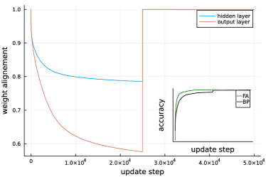
(a)

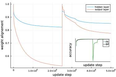
(b)

Figure 1: FA and BP were trained on the same sequence of examples from MNIST starting from the same initial conditions. The graphs show the weight alignment over time between FA and BP for the hidden and output layer. A value of 1 means that FA and BP have the same weights up to a constant factor. LABEL:sub@swap Initially, the two algorithms diverge. After 25000 update steps the weights of the FA network were transferred to the network trained using BP. Following this, they remain aligned, demonstrating that the solution found by FA remains stable under BP. The inset shows the accuracy for both for reference.LABEL:sub@swap2 Same, but at 25000 the FA takes the weight found by BP. This is not stable and the two solutions diverge quickly following the swap. Note how the accuracy of the FA drops immediately following the weight swap, indicating that it is repelled from the loss extremum.

We see from the above equations that for BP the gradient vanishes at each layer when the the derivative of the loss $\left(\partial\mathcal{L}/\partial f_{i}^{(L)}\right)\left(\partial f_{i}^{(L)}/\partial h_{j}^{(L)}\right)$ vanishes for all indices $j$. If the weight matrices are full rank, then this is indeed the only way for the gradient to vanish. We observe that random matrix $\mathbf{R}$ will be maximal rank for as long as elements are chosen iid. Its nullspace vanishes and local extrema of the loss function are therefore also points where the update of the FA pseudo-gradient vanishes. For as long as $\mathbf{R}$ is full rank, then all fixed points of the FA pseudo-gradient will be local extrema of the loss function. As a consequence, the fixed points of FA will be local extrema of the loss function, and local attractors under the BP. This means, that the optimiser in the output layer pushes the entire network, to fixed points of the FA pseudo-gradient. Note that these fixed points need not be attractors of the FA pseudo-gradient. When initialised close to such a fixed point, it is conceivable that FA moves away from the neighbourhood of the fixed point. Indeed, it can be easily seen that this happens (see fig. 1 for an example).

The question is now whether or not there are fixed points that are attractive under the FA pseudo-gradient. The condition for stability is that under the FA update $\Delta^{\textrm{FA}}\mathbf{w}$ the loss does not increase, such that

$$\mathcal{L}\left(\mathbf{m}\left(\mathbf{w}\right)\right)-\mathcal{L}\left(\mathbf{m}\left(\mathbf{w}-\Delta^{\textrm{FA}}\mathbf{w}^{(l)}\right)\right)\geq 0.$$ (4)

Here, we suppressed the label superscripts for clarity and wrote $\mathbf{w}$ instead of $\mathbf{w}^{(l)}$. Assuming the weight update is a small one, we can now expand to first order and obtain

$$\mathbf{m}\left(\mathbf{w}-\Delta^{\textrm{FA}}\mathbf{w}\right)\approx\mathbf{m}\left(\mathbf{w}\right)-\mathbf{m}^{\prime}\left(\mathbf{w}\right)\Delta^{\textrm{FA}}\mathbf{w},$$ (5)

where $\mathbf{m}^{\prime}$ is a three-dimensional matrix with elements $m^{\prime}_{ijk}:=\partial m_{i}/\partial w_{jk}$. We can now further expand the loss function to first order to obtain

$$\mathcal{L}\left(m\left(\mathbf{w}\right)\right)-\mathcal{L}\left(\mathbf{m}\left(\mathbf{w}-\Delta^{\textrm{FA}}\mathbf{w}\right)\right)\approx{\partial\mathcal{L}\over\partial\mathbf{m}}\mathbf{m}^{\prime}(\mathbf{w})\Delta^{\textrm{FA}}\mathbf{w}.$$ (6)

Thus the stability criterion becomes, in first order approximation

$${\partial\mathcal{L}\over\partial\mathbf{m}}\mathbf{m}^{\prime}(\mathbf{w})\Delta^{\textrm{FA}}\mathbf{w}\geq 0$$ (7)

We observe that ${\partial\mathcal{L}\over\partial\mathbf{m}}\mathbf{m}^{\prime}(\mathbf{w})$ is just $\Delta^{\textrm{BP}}\mathbf{w}$, and $\Delta^{\textrm{FA}}\mathbf{w}$ is the FA pseudo-gradient. Furthermore, we see that the rhs of eq. 7 is up to normalisation the alignment measure of the FA update with the BP gradient. Thus, eq. 7 formulates a necessary condition for the stability of a local extremum with respect to the update by the FA pseudo-gradient. This stability criterion states that the alignment measure needs to be positive.

$${\left(\Delta\mathbf{w}\right)^{\textrm{BP}}\cdot\left(\Delta\mathbf{w}\right)^{\textrm{FA}}\over\lVert\Delta\mathbf{w}\rVert^{\textrm{BP}}\cdot\lVert\Delta\mathbf{w}\rVert^{\textrm{FA}}}\geq 0$$ (8)

Put differently, we can now say that gradient alignment is a stability criterion for FA.

2.4 A conjectured mechanism

The FA pseudo-random update rule is a spatially inhomogeneous random walk, whose update steps depend both on the input $\mathbf{x}$ to the network and the current weights $\mathbf{w}$. A priori, there cannot be an expectation that the walker moves along a trajectory that reduces the loss because the FA pseudo-gradient is not a gradient, except in the output layer.

Based on the form of the FA pseudo-gradient, we can still conjecture a mechanism for the walker to find a local extremum of the loss function.

• Initially, the walker moves randomly through parameter space in the input and hidden layers.

• In the output layer, the error is minimised, driving the derivative of the loss function $\partial\mathcal{L}_{i}$ to zero, and hence (as discussed above) towards a fixed point of the FA pseudo-gradient.

• The relevant fixed point may be unstable under the FA pseudo-gradient update rule. In this case, the FA random walker in the input and hidden layers will have a systematic drift, making it impossible for the gradient descent process in the output layer to settle on its local extremum.

• Convergence to a fixed point will only happen when the trajectory towards this fixed point is compatible with the stability criterion for all layers.

There is no guarantee that such a compatible extremum is found. For example, the relevant loss extrema may not be accessible from the initial state, or there may be no extrema for which the stability criterion holds. It could also be that the random walk gets stuck in a region with near-zero update step sizes. For example, the local derivative ${\partial f_{ij}^{(l)}}$ vanishes as weights go to infinity (see A for a discussion of this). This prevents the random walker from exploring the weight space.

2.5 Experiments

In the following, we will try to understand the behaviour of the random walker experimentally by focussing on the particular example of a 3 layer feed-forward neural network trained on the MNIST problem. As we will see below, for this problem and our parameter settings, FA works reasonably well, which makes this a suitable example to gain some insights into how FA works. Note that in what follows the focus is on understanding FA. The NN used and the MNIST benchmark are chosen as illustrative examples. We are not trying to optimise the performance of FA on this task, nor are we attempting to give novel approaches to solve MNIST. Instead, the sole aim of the experiments below is to gain some new insights about FA by observing how it works. The example itself (MNIST) is convenient, because it is easy to solve, but the precise choice of example is to some extent irrelevant, and others could have been used to obtain the same insights.

2.5.1 Alignment

There are two meanings to alignment in FA. ($i$) Weight alignment and ($ii$) gradient alignment. The consensus view in the literature on FA is that FA (somehow) brings about weight alignment, which implies gradient alignment. The latter then drives the FA towards extrema of the loss function. In that sense, FA approximates BP. In this section, we will show some examples where the approach to the local extremum is not driven by weight alignment, at least not during some stages of the simulations.

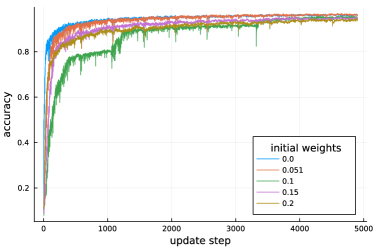
(a)

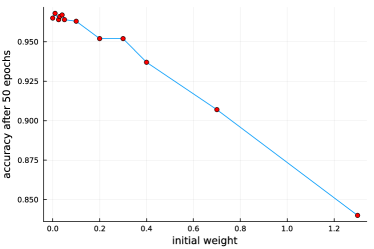
(b)

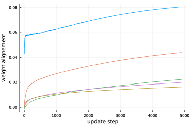
(c)

(d)

Figure 2: The upper panel shows LABEL:sub@alignementd the accuracy as a function of the update step for altogether 10 epochs. LABEL:sub@alignementc The accuracy after 50 epochs as a function of the initial weights (see Methods for an explanation). An approximate linear dependence is discernible. The lower panel shows the LABEL:sub@alignementa weight alignment and LABEL:sub@alignementb gradient alignment for various initial weights as a function of updates. All results are averaged over 3 independent repetitions and used standard parameters (see Methods).

One of the key results by Refinetti et al is that when starting from initially vanishing weights, the update of weights is in the direction of the feedback matrices. If this is true and gradient alignment drives FA learning, then one would expect that small initial weights lead to initially larger alignment than non-vanishing initial weights and that low initial weights lead to faster convergence of FA to a good solution. Our simulations are consistent with this. Fig. 2 shows that there is higher weight alignment (fig. 2c) and gradient alignment (fig. 2d) when initial weights are small. Interestingly, weight alignment remains rather modest in comparison to the gradient alignment. Within 10 epochs, it does not even reach a value of $0.1$. Still, as expected, FA finds good solutions faster when starting with lower weights (fig. 2a). This conclusion also holds in the long run. Even after 50 epochs, the initial conditions matter for the achieved accuracy. The higher the initial weights, the lower the accuracy (see fig. 2b).

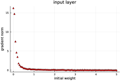
(a)

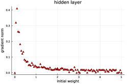
(b)

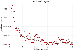
(c)

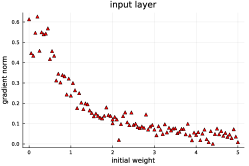
(d)

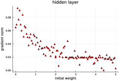
(e)

(f)

Figure 3: LABEL:sub@initialgrada-LABEL:sub@initialgradc The infinite norm of the gradient at the first update step as a function of the initial value scale. LABEL:sub@finalgrada-LABEL:sub@finalgradc Same, but the norm of the gradient after 3 epochs. Note the different scale on the vertical axis, showing how the norm of the gradients has reduced over time. Each point corresponds to a single simulation.

These results are consistent with the view that rapid feedback alignment during early updates is important for the eventual performance of the algorithm. A closer examination, however, reveals some additional complexities, which provide further insight. The first one is highlighted by fig. 3, which shows the norm of the gradient for the input, hidden and output layers after the first update step, so after the algorithm has been presented with the first example of the training set (figs. 3a-3c). The main observation to be made from these figures is that the norm reduces rapidly as the initial weights increase. If we take the norm as an indicator for the step size of the random walker, then this suggests that walkers initialised with high weights suffer from slow speed as a result of small update steps. High weights, therefore mean an effectively reduced learning rate at the beginning of learning. Note the dramatic decrease of the learning rate as the weights start to differ from 0.

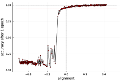
(a)

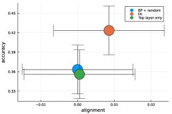
(b)

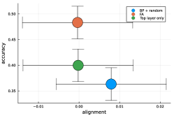
(c)

Figure 4: LABEL:sub@randomdisturb2 We trained a gradient using BP. For the input and hidden layer we perturbed the gradient so that it had an angle relative to the actual gradient. The graph shows the accuracy after one epoch relative to BP. A value of 1 indicates that the perturbed network performs equally well as BP. The red line indicates the performance of a network where only the last layer is trained. The accuracy after 5 updates against the mean gradient alignment for the LABEL:sub@randomdisturbcompare input and LABEL:sub@randomdisturbcompare4 hidden layer. The average is taken over 500 repetitions. The error bars show the standard deviations. For comparison, the perturbed BP is also shown. Clearly, FA does better than the perturbed BP in those examples.

This suggests a new explanation for the improved performance of networks initialised with low weights: FA with initially vanishing weights may perform better because the initial speed of exploration is faster, and hence accuracy can increase over fewer update steps. This means that gradient alignment is not necessarily the only reason why FA performs. At least, we have shown one example which suggests a different explanation. We hasten to add that the two explanations are not mutually exclusive.

This begs now the question whether or not gradient alignment drives accuracy, or whether gradient alignment is merely a by-product of the FA dynamics. This is best explored during the earliest stages of learning, before a substantial alignment has formed. In order to be able to investigate this, we first need to understand the relationship between gradient alignment and loss. To this end, we generated a baseline curve as follows: We used the BP algorithm to train the network for 1 epoch on the MNIST dataset. However, each time the gradient was computed in the hidden and input layer, we randomly perturbed it, such that the actual gradient used for updating the weights was different from the gradient determined by BP. We could then, for each experiment, determine the alignment between the true gradient and the perturbed gradient. We did this systematically in fig. 4a, which shows the accuracy after 1 epoch as a function of the average alignment. By design, this set of experiments isolates the effect of the gradient alignment, while all other details of the algorithm are left the same. The figure also shows in red, the baseline of a multi-layer network where only the last layer is trained, whereas all other layers remain at the initial weights.

A number of observations can be made. Firstly, the accuracy of the network intersects the red line for an alignment of 0. In this case, the perturbed gradients are orthogonal to the actual gradients one would obtain from BP which means that weight updates do not have an overall drift either into the direction of better accuracy or away from it. Consistently, the accuracy of the network then corresponds to simulations where only the output layer is trained (indicated by the red line in fig. 4a). Further increasing the alignment, only improves the performance a little bit, reflecting the well known fact that training only the output layer leads to high accuracies in many cases. On the other hand, for negative alignments, the performance quickly drops to random guessing, which corresponds to an accuracy of $0.1$. (Note that the effect of updating against the gradient is a randomisation of the performance, rather than guiding the network to an accuracy below $0.1$, which would require updating the weights of the output layer against the gradient as well.) A further observation to be made from this is that the gradient descent process operating at the output layer cannot settle on a minimum when the weights in the lower layers have a systematic drift in one direction.

Fig. 4a shows how alignment (or rather misalignment) with the BP gradient impacts learning performance. We can now use this to see whether the FA performance is driven solely by the alignment of the pseudo-gradient or whether there is more to it. If FA performs exactly as well as the perturbed BP with the same alignment, then we know that gradient alignment is driving performance. If, on the other hand, it performs better, then there is some additional driver.

Fig. 4b gives some relevant insight. It shows the performance as a function of the average alignment for FA, gradient perturbed BP and and a network where only the top layer is trained. Fig. 4b and 4c compare the performance of the three algorithms after 5 updates against the alignment of the input and hidden layer. This shows that, for similar alignment, FA does much better than the other two algorithms. This suggests two things: ($i$) Gradient alignment is not the only driver of performance of FA, at least not during early stages. ($ii$) The performance of the FA during early stages is not entirely driven by the gradient descent in the output layer, but the update of the input and hidden layer does add to performance.

2.5.2 Alignment can reduce performance

So far, we have established that alignment between the gradient and pseudo-gradient is not driving performance during early stages of learning. We will now show that alignment is not sufficient for performance, even during later stages, and indeed can be outright detrimental.

Fig. 5 shows, as an example, a set of three different simulations of FA with identical hyper-parameters. The only difference between them is the initialisation of the weights. The blue line is just a standard simulation, with weights being initially drawn from a normal distribution before being scaled by $0.05$. The green simulation is the same, but the signs of the initial weights were set equal to the entries of the corresponding feedback matrices. As a consequence, there is a large initial alignment between the weights and the feedback matrices. Finally, the red points show the results for a simulation where the initial weights were set to be identical to the feedback matrices before being scaled by $0.05$. For all three simulations, we drew the elements of the feedback matrices from a normal distribution, rather than from the set $\{-1,1\}$. We did this so that the initial weights in the blue simulation are statistically indistinguishable from the other two simulations, while the initial alignment between the weights is different in the three cases. By construction, the blue simulation is unaligned initially, the red simulation is perfectly aligned and the green simulation is somewhere in between those two cases.

(a)

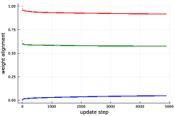
(b)

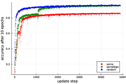
(c)

Figure 5: Feedback alignment, with initial weights chosen at random (blue), randomly but the sign of each element was the same as the feedback matrix (green) and exactly the same as the feedback matrix (red). We show LABEL:sub@angle the angle between the true gradient and the feedback gradient of the hidden layer, LABEL:sub@angle the alignment between the weights of the hidden layer and the feedback matrix, LABEL:sub@accuracy the accuracy over time. There is no trend between higher alignment and better accuracy, or better increase of accuracy. Each point represents a value taken after an update step. Altogether, the simulations here represent 10 epochs.

We find from the simulations presented in fig. 5, as expected, that good weight alignment translates to high gradient alignment. The key message of the graph is that the initially unaligned simulation performs best, amongst the three runs. While we are not claiming that high gradient alignment is always detrimental, from this single example we can still draw two conclusions: ($i$) Weight alignment is not a necessary condition for performance of the FA algorithm. ($ii$) High gradient alignment is not sufficient for performance of the FA algorithm.

While the performance of the red simulation is still good in the sense that it is apparently learning something, it is possible to construct examples of FA networks that have almost perfect alignment throughout, but learn nothing (data not shown). The simplest way to do this is to use feedback matrices that are initialised by randomly drawing elements from the set $\{-1,1\}$, and set the initial weights equal to the feedback matrices. These initial conditions are not conducive to algorithm performance, and the network does not train well. Altogether, we find, that gradient alignment is not always sufficient to explain the performance of FA algorithms. We could show at least one example, where other mechanisms are required.

3 Discussion

At a first glance, FA and DFA should not work. By replacing a key term in the update equation, the gradient descent of BP is effectively transformed into a random walk in weight-space. The key observation that had been made early on was that this random walk aligns with the “true” BP gradient. In the literature this alignment is commonly assumed to be the driver for the performance of the FA algorithm. It remains unclear, however, why FA aligns. Existing mathematical models only cover special simplified cases of neural networks. They suggest that the update dynamics of FA leads to weight alignment, which then implies gradient alignment. In that sense, FA approximates the true gradient. However, weight alignment is typically much weaker than gradient alignment. This suggests that some other explanations are required.

Our theoretical results suggest a somewhat different view: FA is not approximating BP at all, and indeed does not descend or ascend the gradient of a loss function or an approximation thereof. It is not “learning” in the sense one normally understands this term. Instead, it performs a random walk in weight space. It works based on the following conjectured mechanism: At the output layer, the gradient descend process drives the network as a whole towards a fixed point, corresponding to a vanishing gradient of the loss function. Many of those fixed points are unstable for the random walker and the updates in the hidden and input layer will drive the network away from the fixed point, until a fixed point is found for which the stability criterion is valid. Then, the network will converge towards this fixed point.

There is no guarantee that FA finds extrema that are compatible with the alignment criterion. Failure to do so could be either because there are no compatible extrema, or because FA is initialised in a part of parameter space from which it cannot find a route to compatible fixed points. The latter scenario could realise when extrema of the loss function are sparse in parameter space or when the weights are initialised in an area that has small update steps, for example for large initial weights. The often cited failure of FA for convolutional neural networks is likely a consequence of the sparseness of loss extrema for those networks.

Throughout this article we concentrated on FA, but clearly the conclusions can be transferred directly to DFA. The only difference between FA and DFA is that in the latter each layer performs an independent walk, whereas in FA the training process is a single random walker in a higher dimensional space. The basic mechanism of how DFA finds extrema remains the same as in the case of FA.

Some open questions remain. The first one relates to the distribution of local extrema of the loss function in parameter space. In particular, it may be that for certain types of problems there are conditions that guarantee that FA and DFA find local extrema or alternatively, that they do not find such extrema (as seems to be the case for convolutional neural networks). There is also a lack of theoretical understanding of spatially inhomogeneous random walks. In order to come to a complete theoretical description of FA, we need a sound justification of how and under which conditions random walks approach fixed points.

4 Methods

Unless otherwise stated, we used a feed forward multi-layer perceptron with an input/hidden layer of 700/1000 neurons. The size of the network was chosen to be large, while still being fast to execute. Our results are not sensitive to variations of the size of the network, although classification performance clearly is. Throughout, we used $\tanh$ as the activation function; we also experimented with relu which led to qualitatively the same results (data not shown). For the final layer we used the softmax function and as a loss function we used the cross-entropy. The batch size was chosen to be 100 and the learning rate was set to $0.05$. Again, our results are not sensitive to those parameters.

Unless stated otherwise, feedback matrices were chosen randomly by drawing matrix elements from the set $\{-1,1\}$. We found FA not to be overly sensitive to the particular choice of this set. However, we found algorithm performance to depend on it to some extent. The particular choice we made gives good performance, but we made no attempt to choose the optimal one.

For all layers, initial weights were drawn from a normal distribution and then scaled with a weight scaling factor, resulting in both negative and positive weights. If the factor is zero, then all weights were initially zero. The larger the factor, the larger the (absolute value of) initial weights.

All simulations were done using Julia (1.8.5) Flux for gradient computations and network construction, and CUDA for simulations on GPUs. Throughout no optimisers were used. Weight updates were made by adding the gradient, scaled by the learning rate, to the weights. The networks were trained on the MNIST dataset as included with the Flux library. Whenever an accuracy is reported it was computed based on the test-set of the MNIST dataset.

Appendix A Two basic properties of FA

A.1 Vanishing weights are unstable for some activation functions

As pointed out by [19], for BP the initialisation $w_{ij}=0$ results in a deadlock, in the sense that irrespective of the inputs, the weight updates will always vanish. This can be seen clearly from eq. 2.2: For each layer, the matrices $\partial h_{i}^{(l)}/\partial f_{j}^{(l)}$ evaluate to $w_{ij}^{(l)}$. Therefore, trivially the weight updates will be vanishing as well. In the case of FA, these expressions are replaced by non-vanishing random terms. With this change, the update of the $l=1$ layer,

$$\Delta w_{pq}=\partial\mathcal{L}_{i}B_{ij}^{(1)}f_{jp}^{(1)}x_{q}$$

is no longer proportional to the weights, and hence not identically zero. Upon the first update, the weights of the input layer will typically be non-vanishing, such that the update of the $l=2$ layer will be non-vanishing as well. After $L$ updates, all layers may have weights that are different from 0. The initialisation $w_{ij}=0$ is therefore not a fixed points of the FA pseudo-update rule.

A.2 Weight increments tend to zero for large weights for some choices of activation function

The behaviour for large weights depends on the activation functions that are chosen. It is therefore not possible to make general statements. However, many popular choices for these functions will lead to vanishing weight updates. We restrict the discussion to the choices made here. The derivative of the softmax function $\mathbf{\sigma}(x_{1},\ldots,x_{n})$ can be seen to vanish at infinite weights. The derivative of the first component of the softmax function with respect to $x_{1}$ gives

$${\partial\sigma_{1}\over\partial x_{1}}={\exp(x_{1})\over\sum_{i}\exp(x_{i}}-\left({\exp(x_{1})\over\sum_{i}\exp(x_{i})}\right)^{2}.$$

It is straightforward to confirm that as $\max(x_{i})\rightarrow\infty$ the first and the second term simultaneously either go to 0 or 1. Similarly, for $k\neq 1$

$${\partial\sigma_{1}\over\partial x_{k}}=-{\exp(x_{1})\over\sum_{i}\exp(x_{k})}{\exp(x_{i})\over\sum_{i}\exp(x_{i})}.$$

Here at least one of the two terms vanishes for as long as the difference between any two $x_{j}$ is sufficiently large.

From the shape of the $\tanh(x)$ it is clear that its derivative vanishes with $x\rightarrow\pm\infty$. The same is not true, however, for relu which has a constant derivative.

We conclude that for networks that use the softmax function weight updates will vanish in the regime of large weights when the softmax function is used in the last layer.

References

- [1] D. E. Rumelhart, G. E. Hinton, R. J. Williams, Learning representations by back-propagating errors, nature 323 (6088) (1986) 533–536.
-
[2]
Y. LeCun, C. Cortes, MNIST
handwritten digit database (2010) [cited 2016-01-14 14:24:11].
URL http://yann.lecun.com/exdb/mnist/ - [3] J. Launay, I. Poli, F. Boniface, F. Krzakala, Direct feedback alignment scales to modern deep learning tasks and architectures, in: Proceedings of the 34th International Conference on Neural Information Processing Systems, NIPS’20, Curran Associates Inc., Red Hook, NY, USA, 2020.
- [4] Z. Huo, B. Gu, Q. Yang, H. Huang, Decoupled parallel backpropagation with convergence guarantee (2018). arXiv:1804.10574.
-
[5]
B. Crafton, A. Parihar, E. Gebhardt, A. Raychowdhury,
Direct
feedback alignment with sparse connections for local learning, Frontiers in
Neuroscience 13 (2019).
doi:10.3389/fnins.2019.00525.
URL https://www.frontiersin.org/articles/10.3389/fnins.2019.00525 - [6] B. Crafton, A. Parihar, E. Gebhardt, A. Raychowdhury, Direct feedback alignment with sparse connections for local learning, Frontiers in Neuroscience 13 (2019) 525.
- [7] D. Han, H.-j. Yoo, Direct feedback alignment based convolutional neural network training for low-power online learning processor, in: 2019 IEEE/CVF International Conference on Computer Vision Workshop (ICCVW), 2019, pp. 2445–2452.
- [8] S. Sarwar, G. Srinivasan, B. Han, P. Wijesinghe, A. Jaiswal, P. Panda, A. Raghunathan, K. Roy, Energy efficient neural computing: A study of cross-layer approximations, IEEE Journal on Emerging and Selected Topics in Circuits and Systems 8 (4) (2018) 796–809. doi:10.1109/JETCAS.2018.2835809.
-
[9]
E. Strubell, A. Ganesh, A. McCallum,
Energy and policy considerations for
deep learning in NLP, in: Proceedings of the 57th Annual Meeting of the
Association for Computational Linguistics, Association for Computational
Linguistics, Florence, Italy, 2019, pp. 3645–3650.
doi:10.18653/v1/P19-1355.
URL https://aclanthology.org/P19-1355 - [10] E. O. Neftci, C. Augustine, S. Paul, G. Detorakis, Event-driven random back-propagation: Enabling neuromorphic deep learning machines, Frontiers in Neuroscience 11 (2017).
- [11] M. Davies, N. Srinivasa, T. Lin, G. Chinya, Y. Cao, S. Choday, G. Dimou, P. Joshi, N. Imam, S. Jain, Y. Liao, C. Lin, A. Lines, R. Liu, D. Mathaikutty, S. McCoy, A. Paul, J. Tse, G. Venkataramanan, Y. Weng, A. Wild, Y. Yang, H. Wang, Loihi: A Neuromorphic Manycore Processor with On-Chip Learning, IEEE Micro 38 (1) (2018) 82–99. doi:10.1109/MM.2018.112130359.
- [12] L. Plana, D. Clark, S. Davidson, S. Furber, J. Garside, E. Painkras, J. Pepper, S. Temple, J. Bainbridge, Spinnaker: Design and implementation of a gals multicore system-on-chip, J. Emerg. Technol. Comput. Syst. 7 (4) (2011) 17:1–17:18. doi:10.1145/2043643.2043647.
- [13] G. Hinton, The forward-forward algorithm: Some preliminary investigations (2022). arXiv:2212.13345.
- [14] T. P. Lillicrap, D. Cownden, D. B. Tweed, C. J. Akerman, Random synaptic feedback weights support error backpropagation for deep learning, Nature Communications 7 (2016).
- [15] A. Nøkland, L. H. Eidnes, Training neural networks with local error signals, in: K. Chaudhuri, R. Salakhutdinov (Eds.), Proceedings of the 36th International Conference on Machine Learning, Vol. 97 of Proceedings of Machine Learning Research, PMLR, 2019, pp. 4839–4850.
-
[16]
A. Sanfiz, M. Akrout, Benchmarking the
accuracy and robustness of feedback alignment algorithms, CoRR
abs/2108.13446 (2021).
arXiv:2108.13446.
URL https://arxiv.org/abs/2108.13446 -
[17]
D. Zhao, Y. Zeng, T. Zhang, M. Shi, F. Zhao,
Glsnn:
A multi-layer spiking neural network based on global feedback alignment and
local stdp plasticity, Frontiers in Computational Neuroscience 14 (2020).
doi:10.3389/fncom.2020.576841.
URL https://www.frontiersin.org/articles/10.3389/fncom.2020.576841 - [18] J. Launay, I. Poli, F. Krzakala, Principled training of neural networks with direct feedback alignment (06 2019).
- [19] M. Refinetti, S. D’Ascoli, R. Ohana, S. Goldt, Align, then memorise: the dynamics of learning with feedback alignment, in: International Conference on Machine Learning, 2021, pp. 8925–8935.
-
[20]
D. Saad, S. A. Solla,
Exact solution
for on-line learning in multilayer neural networks, Phys. Rev. Lett. 74
(1995) 4337–4340.
doi:10.1103/PhysRevLett.74.4337.
URL https://link.aps.org/doi/10.1103/PhysRevLett.74.4337 - [21] F. Xia, J. Liu, H. Nie, Y. Fu, L. Wan, X. Kong, Random walks: A review of algorithms and applications, IEEE Transactions on Emerging Topics in Computational Intelligence 4 (2) (2020) 95–107. doi:10.1109/TETCI.2019.2952908.