Learning Test-Mutant Relationship for Accurate Fault Localisation

Abstract

Context: Automated fault localisation aims to assist developers in the task of identifying the root cause of the fault by narrowing down the space of likely fault locations. Simulating variants of the faulty program called mutants, several Mutation Based Fault Localisation (MBFL) techniques have been proposed to automatically locate faults. Despite their success, existing MBFL techniques suffer from the cost of performing mutation analysis after the fault is observed.

Method: To overcome this shortcoming, we propose a new MBFL technique named SIMFL (Statistical Inference for Mutation-based Fault Localisation). SIMFL localises faults based on the past results of mutation analysis that has been done on the earlier version in the project history, allowing developers to make predictions on the location of incoming faults in a just-in-time manner. Using several statistical inference methods, SIMFL models the relationship between test results of the mutants and their locations, and subsequently infers the location of the current faults.

Results: The empirical study on Defects4J dataset shows that SIMFL can localise 113 faults on the first rank out of 224 faults, outperforming other MBFL techniques. Even when SIMFL is trained on the predicted kill matrix, SIMFL can still localise 95 faults on the first rank out of 194 faults. Moreover, removing redundant mutants significantly improves the localisation accuracy of SIMFL by the number of faults localised at the first rank up to 51.

Conclusion: This paper proposes a new MBFL technique called SIMFL, which exploits ahead-of-time mutation analysis to localise current faults. SIMFL is not only cost-effective, as it does not need a mutation analyse after the fault is observed, but also capable of localising faults accurately.

1 Introduction

Fault Localisation (FL) is the problem of diagnosing the root cause of the fault by highlighting a few program elements likely to be responsible for the fault. It is an expensive debugging activity as it involves a human inspection to point out the suspicious locations in Program Under Test (PUT) based on the understanding of the root cause. As such, the necessity of developing automated localisation techniques has received increasing attention [1, 2, 3, 4, 5, 6], not only to help human developers but also to be adopted as a prerequisite for Automated Program Repair (APR) [7, 8, 9].

Mutation Based Fault Localisation (MBFL) [10, 11, 12, 13, 14] is one such way that utilises mutation analysis. Mutants are program variants made up of a single or multiple syntactic operator(s), designed to simulate the real faults. Various empirical studies [15, 16, 17] have provided evidence of a correlation between detection of the mutants and detection of the faults. Exploiting this, Metallaxis [12, 13] considers the location of the mutants that have similar failing patterns with the faults as candidate locations of the fault. MUSE [10] and MUSEUM [11] have taken different approaches that reward the mutants causing partial fixes and devalue the mutants making an additional failure.

Although the usefulness of MBFL techniques has long been demonstrated, the substantial cost of mutation analysis has hampered their practical applications. The cost reduction techniques for MBFL are in line with the cost reduction techniques for traditional mutation testing: random sampling of the mutants [13] and higher-order mutants [18]. They have reduced the number of mutants and test executions, but still they are not suitable for large systems like Google’s on which more than ten million test executions take place everyday [19]. To avoid this, recent advances employ the context of Continuous Integration (CI) [20]: predictive mutation testing techniques [21, 22, 23] aim to predict mutation testing results without mutant executions by learning static and dynamic features of mutants from earlier version of the project.

In this work, we propose SIMFL (Statistical Inference for Mutation-based Fault Localisation), an MBFL technique that operates in the CI context. Unlike other FL techniques that undertake work on locating faults a posteriori, SIMFL uses a kill matrix computed on earlier version of the PUT, which therefore amortises the costs of mutation analysis that has been done after the actual faults are observed. The kill matrix records the test results of each mutant, and SIMFL uses it to relate the locations of mutants and faults: if the mutants were killed by the similar set of tests that detects the faults, SIMFL values such mutants and presumes their locations as likely locations of the faults. To model this kind of predictive inferences, SIMFL makes use of several statistical inference techniques such as Bayesian inference, probabilistic coupling, and more sophisticated models such as Logistic Regression or Multi-Layer Perceptron. Once building a predictive model in advance, SIMFL produces a rank of suspicious program elements by feeding the test results of the fault into the model.

We conduct extensive empirical experiments on SIMFL in three different use cases. Using the real-world fault dataset, Defects4J v1.3.1 [24], and Major mutation tool [25], SIMFL places 113 faults on the first rank out of 224 faults and outperformed existing MBFL techniques. Even if SIMFL is built on the predicted kill matrix by Seshat [23], it localises 95 faults on the first rank out of 194 faults, showing its practical value. As SIMFL does not require the execution of mutants, it shows a significant improvement in efficiency over other MBFL techniques and it is even faster than running a entire test suite once. We also investigate how much SIMFL is affected by mutant sampling and the results show that SIMFL retains 80% of localisation accuracy when it uses only 10% of mutants. Lastly, we demonstrate the assumption that subsumed mutants [26, 27] would disrupt the scoring functions of SIMFL. The evaluation of SIMFL models after eliminating the subsumed mutants reveals that the number of faults localised at the first rank increases up to 51.

This paper is an extended version of the conference paper [28]. The contributions of the conference paper are as follows:

• We present SIMFL, an MBFL technique that infers the location of faults based on the mutation analysis performed before the faults are observed. This allows SIMFL to significantly amortise the costs of mutation analysis, and the experiments on Defects4J dataset showed that SIMFL achieves better localisation accuracy than existing MBFL techniques.

• We introduce several modelling schemes of SIMFL using statistical inferences and machine learning techniques. We not only compare their effectiveness but also provide the empirical evidence of the impacts of model viability and mutant sampling.

• We further investigate the impact of test granularity and mutant filtering based on the kill reason (e.g., exception). The in-depth observation on the relationship with other FL techniques open up a positive hybridisation of SIMFL and other techniques.

The paper has been extended with the following technical contributions:

• We have added a new use scenario of SIMFL using a predicted kill matrix of Seshat, which is not dependent on pre-existence of failing tests.

• We have proposed a new ranking model based on probabilistic coupling. We apply a definition of mutant-fault coupling that values the mutants tightly coupled to the fault.

• We have conducted a new experiment to investigate the execution time of SIMFL compared to other MBFL techniques.

• We have added new faults introduced in Defects4J v2.0.0 in our study, to further validate our conclusion with a larger fault dataset.

• We have investigated the effects of removing the subsumed mutants. We observed that the subsumed mutants disturb and inflate the method-level aggregation of FL scores by SIMFL. The new experiment showed that eliminating them significantly improves the effectiveness of SIMFL.

• We have made a raw data publicly available at https://figshare.com/s/954a7f27bb0e08b009f8 for the replication of our experiments.

The rest of the paper is organised as follows. Section 2 details how the mutation analysis results are formulated for fault localisation. Section 3 introduces three use scenarios of SIMFL, research questions, and experimental settings. Section 4 answers each research question and Section 5 provides discussions. Section 6 presents threats to validity. Section 7 introduces related work and Section 8 concludes.

2 Methodology

Intuitively, the underlying assumption of SIMFL is that, for a test that has killed the mutants located on a specific program element, the same program element should be identified as the suspicious location when the same test later fails again. This is based on the coupling effect hypothesis in mutation testing: essentially we simulate the occurrence of real faults with artificial faults with known locations, i.e., mutants, and build predictive models for actual future faults. This section describes the models and the statistical inference techniques used by SIMFL.

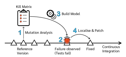
Figure 1: Expected use case scenario of SIMFL

Figure 1 depicts the expected use case scenario of SIMFL, which includes four stages:

1. Perform mutation analysis for a version of SUT, and produce the kill matrix. The version is called the reference version.

2. While testing a subsequent version, a failure is observed.

3. Using the information of which test case(s) failed, as well as the kill matrix, build a predictive model for fault localisation.

4. Guided by the localisation result, patch the fault.

Table 1: Key Symbols

Symbol	Meaning
$\mathbf{P}$	Program under test.
$\mathbf{T}$	Entire test suite.
$\mathbf{T}_{f}$	Set of failing tests on a given program.
$\mathbf{T}_{p}$	Set of passing tests on a given program.
$\mathbf{K}$	Kill matrix.
$m$	Mutant.
$e$	Program element.
$\mathbf{K}_{m}$	Set of tests that kill $m$.
$\mathbf{X}_{e}$	Set of mutants located on $e$.
$M_{e}$	Event that $e$ is mutated.
$F_{t}$	Event that a test case $t$ fails on a given program.
$P_{t}$	Event that a test case $t$ passes on a given program.
$F_{\mathbf{T}_{f}}$	Event that all tests in $\mathbf{T}_{f}$ fail on a given program.
$Pr\left(M_{e}\right)$	Probability of $e$ is mutated.
${\color[rgb]{0,0,0}Pr}\left(F_{t}\mid M_{e}\right)$	Probability of $t$ fails when $e$ is mutated.

2.1 Mutation Analysis

Table 2: An Example Kill Matrix

Class	Method	Mutants	Test Results				0-1 Vectors
			$t_{1}$	$t_{2}$	$t_{3}$	$t_{4}$	of $t_{1},t_{2},t_{3},t_{4}$
com. acme. Foo	getType	n.isName() $\mapsto$ true ($m_{1}$)	✗	✗	✓	✓	$\left(1,1,0,0\right)$
		n.isName() $\mapsto$ false ($m_{2}$)	✓	✓	✗	✓	$\left(0,0,1,0\right)$
		bFlag or isInferred $\mapsto$ isInferred ($m_{3}$)	✓	✗	✗	✓	$\left(0,1,1,0\right)$
	resolveType	param.isTemplateType() $\mapsto$ true ($m_{5}$)	✓	✗	✓	✓	$\left(0,1,0,0\right)$
		resolvedType() $\mapsto$ deleted ($m_{6}$)	✗	✗	✗	✓	$\left(1,1,1,0\right)$

We perform mutation analysis on the reference version of a program $\mathbf{P}$ with a test suite $\mathbf{T}$, and compute a kill matrix $\mathbf{K}$, which contains a complete report of all tests executed on all mutants. An example kill matrix is shown in Table 2: the mutant $m_{1}$ located in the method getType is killed by the test cases $t_{1}$ and $t_{2}$, whereas $m_{2}$ is only killed by $t_{3}$. We list the key symbols in Table 1 to aid in the understanding of the formulae we will introduce in the following.

Let $\mathbf{K}_{m}$ denote a set of tests that kill mutant $m$, let $\mathbf{X}_{e}$ be a set of mutants located on a program element $e\in\mathbf{P}$, let $M_{e}$ be an event that $e$ is mutated, and let $F_{t}$ be an event that a test case $t$ fails on a given program. Based on the kill matrix $\mathbf{K}_{m}$, we can approximate the probability of test case $t$ killing the mutants located on the program element $e$ as follows:

$${\color[rgb]{0,0,0}Pr}\left(F_{t}\mid M_{e}\right)\simeq\frac{|\left\{m\in\mathbf{X}_{e}:t\in\mathbf{K}_{m}\right\}|}{|\mathbf{X}_{e}|}$$ (1)

Note that this is strictly an approximation based on the observed kill matrix because it is impossible to produce and evaluate all possible mutants. The value of $Pr\left(M_{e}\right)$ is the ratio of the number of all possible mutants on $e$ to the number of all possible mutants on $\mathbf{P}$; for ${\color[rgb]{0,0,0}Pr}\left(F_{t}\mid M_{e}\right)$, we need to calculate the number of all possible mutants in $e$ that are killed by $t$. Neither is feasible. Consequently, we assume that we can analyse a finite set of mutants that allow us to approximate Equation 1. We note that test failure history over the project lifetime can be used to approximate both $P(M_{e})$ (i.e., the probability that method $e$ is faulty after a commit) and $P(F_{t}|M_{e})$ (i.e., the probability that test $t$ fails when method $e$ is faulty). Such historical approximation may be more accurate, but would require high traceability between test failures and code changes throughout the project history.

Next, using Bayes’ rule, we calculate the revised probability of the event that the program element $e$ has been mutated, given that the test case $t$ fails:

$$\begin{split}{\color[rgb]{0,0,0}Pr}\left(M_{e}\mid F_{t}\right)&=\frac{{\color[rgb]{0,0,0}Pr}\left(F_{t}\mid M_{e}\right){\color[rgb]{0,0,0}Pr}\left(M_{e}\right)}{{\color[rgb]{0,0,0}Pr}\left(F_{t}\right)}\\ &\simeq{\color[rgb]{0,0,0}Pr}\left(\text{fault exists in }e\mid F_{t}\right)\end{split}$$ (2)

We argue that, if real faults are coupled to mutants, the probability above can approximate the likelihood that the fault is located on the program element $e$, when $t$ is a failing test case in the future. Our approximation assumes that tests are equally sensitive to mutants and real bugs. This allows us to make ranking models that sort the program elements in descending order of the probability.

2.2 Ranking Models Based on Bayes’ Rule

We regard the probability in Equation 2 as the quantitative score representing how suspicious the program element $e$ is for the failure observed via the failure of $t$. This section presents the formulations of ranking models based on the scores as well as more refined inference models based on kill matrix data.

2.2.1 Exact Matching (EM)

This model is an extension of Equation 2 to a set of test cases. Let $\mathbf{T}=\{t_{i}:1\leq i\leq n\leq n^{\prime}\}$ be the test set, which consists of two disjoint sets: $\mathbf{T}_{f}=\{t_{1},\dots,t_{n}\}$ is the set of failing test cases, and $\mathbf{T}_{p}=\mathbf{T}\setminus\mathbf{T}_{f}$ is the set of passing tests, on the faulty program. While there can be many different formulations of ranking models based on a set of test cases, we start by treating the set of all observed failures, $F_{\mathbf{T}_{f}}$, as a conjunctive event of individual test case failures, i.e., $F_{\mathbf{T}_{f}}=F_{t_{1}}\cap\dots\cap F_{t_{n}}$. Our goal is to find the faulty program element $e_{i}\in\mathbf{P}$ with the highest probability of being the cause of the observed failure symptoms, that is, ${\color[rgb]{0,0,0}Pr}\left(M_{e_{i}}\mid F_{\mathbf{T}_{f}}\right)$. It follows that:

$$\begin{split}\mathop{\mathrm{argmax}}_{i}{\color[rgb]{0,0,0}Pr}\left(M_{e}\mid F_{\mathbf{T}_{f}}\right)&=\mathop{\mathrm{argmax}}_{i}\frac{{\color[rgb]{0,0,0}Pr}\left(F_{\mathbf{T}_{f}}\mid M_{e}\right){\color[rgb]{0,0,0}Pr}\left(M_{e}\right)}{{\color[rgb]{0,0,0}Pr}\left(F_{\mathbf{T}_{f}}\right)}\end{split}$$ (3)

The denominator in Equation 3, ${\color[rgb]{0,0,0}Pr}\left(F_{\mathbf{T}_{f}}\right)$, can be ignored without affecting the order of ranking based on this score, because it is not related to a specific program element. Expanding the numerator yields the following:

$$\begin{split}&\mathop{\mathrm{argmax}}_{i}{\color[rgb]{0,0,0}Pr}\left(F_{\mathbf{T}_{f}}\mid M_{e_{i}}\right){\color[rgb]{0,0,0}Pr}\left(M_{e_{i}}\right)\\ &=\mathop{\mathrm{argmax}}_{i}{\color[rgb]{0,0,0}Pr}\left(F_{t_{1}}\cap\dots\cap F_{t_{n}}\mid M_{e_{i}}\right){\color[rgb]{0,0,0}Pr}\left(M_{e_{i}}\right)\\ &=\mathop{\mathrm{argmax}}_{i}\frac{|\{m\in\mathbf{X}_{e_{i}}:\{t_{1},\dots,t_{n}\}=\mathbf{K}_{m}\}|}{|\mathbf{X}_{e_{i}}|}{\color[rgb]{0,0,0}Pr}\left(M_{e_{i}}\right)\\ &=\mathop{\mathrm{argmax}}_{i}\frac{|\{m\in\mathbf{X}_{e_{i}}:\mathbf{T}_{f}=\mathbf{K}_{m}\}|}{|\mathbf{X}_{e_{i}}|}\frac{|\mathbf{X}_{e_{i}}|}{|\mathbf{X}_{\mathbf{P}}|}\\ &=\mathop{\mathrm{argmax}}_{i}\frac{|\{m\in\mathbf{X}_{e_{i}}:\mathbf{T}_{f}=\mathbf{K}_{m}\}|}{|\mathbf{X}_{\mathbf{P}}|}\\ &=\mathop{\mathrm{argmax}}_{i}|\{m\in\mathbf{X}_{e_{i}}:\mathbf{T}_{f}=\mathbf{K}_{m}\}|\end{split}$$ (4)

Intuitively, Equation 4 counts the mutants on $e$ that cause the same set of test cases to fail as the symptom of the actual fault, $F_{\mathbf{T}_{f}}$. We call this model the Exact Matching (EM) model with failing test cases, denoted by EM(F).

Alternatively, we can include passing tests in the pattern matching as well. Let $P_{t}$ be an event that a test case $t$ passes on a given program, then Equation 4 changes as follows:

$$\begin{split}&\mathop{\mathrm{argmax}}_{i}{\color[rgb]{0,0,0}Pr}\left(F_{\mathbf{T}_{f}}\cap P_{\mathbf{T}_{p}}\mid M_{e_{i}}\right){\color[rgb]{0,0,0}Pr}\left(M_{e_{i}}\right)\\ &=\mathop{\mathrm{argmax}}_{i}{\color[rgb]{0,0,0}Pr}\left(F_{t_{1}}\cap\dots\cap F_{t_{n}}\cap P_{t_{n+1}}\cap\dots\cap P_{t_{n^{\prime}}}\mid M_{e_{i}}\right){\color[rgb]{0,0,0}Pr}\left(M_{e_{i}}\right)\\ &=\mathop{\mathrm{argmax}}_{i}|\{m\in\mathbf{X}_{e_{i}}:\mathbf{T}_{f}=\mathbf{K}_{m}\wedge\mathbf{T}_{p}=\mathbf{T}\setminus\mathbf{K}_{m}\}|\end{split}$$ (5)

Similarly to EM(F), this model is called EM(F+P): it counts the mutants on $e$ that cause the same set of test cases to fail and pass exactly as the symptom of the actual fault. If, for example, a test case $t$ passed under the actual fault, EM(F+P) model will not count any mutants that are killed by $t$.

2.2.2 Partial Matching (PM)

The Exact Matching (EM) models lose any partial matches between the symptom and the mutation results. Suppose two test cases, $t_{1}$ and $t_{2}$, failed under the actual fault, but only $t_{1}$ killed a mutant on the faulty program element, i.e., $\exists t_{1},t_{2}\in\mathbf{T}_{f},t_{1}\in\mathbf{K}_{m}\land t_{2}\notin\mathbf{K}_{m}$. The information that $t_{1}$ kills a mutant on the location of the fault is lost, simply because $t_{2}$ failed to do the same. To retrieve this partial information, we propose two additional models based on partial matches: a multiplicative partial match model and an additive partial match model.

• PM^∗(F): Multiplicative Partial Match Model w/ Failing Tests

  $$\begin{split}&\mathop{\mathrm{argmax}}_{i}\prod_{t\in\mathbf{T}_{f}}\left({\color[rgb]{0,0,0}Pr}\left(M_{e_{i}}\mid F_{t}\right)+\epsilon\right)\\ &=\mathop{\mathrm{argmax}}_{i}\prod_{t\in\mathbf{T}_{f}}\frac{{\color[rgb]{0,0,0}Pr}\left(F_{t}\mid M_{e_{i}}\right){\color[rgb]{0,0,0}Pr}\left(M_{e_{i}}\right)}{{\color[rgb]{0,0,0}Pr}\left(F_{t}\right)}+\epsilon\\ &=\mathop{\mathrm{argmax}}_{i}\prod_{t\in\mathbf{T}_{f}}{\color[rgb]{0,0,0}Pr}\left(F_{t}\mid M_{e_{i}}\right){\color[rgb]{0,0,0}Pr}\left(M_{e_{i}}\right)+\epsilon\\ &=\mathop{\mathrm{argmax}}_{i}\prod_{t\in\mathbf{T}_{f}}\frac{|\{m\in\mathbf{X}_{e_{i}}:t\in\mathbf{K}_{m}\}|}{|\mathbf{X}_{e_{i}}|}\frac{|\mathbf{X}_{e_{i}}|}{|\mathbf{X}_{\mathbf{P}}|}+\epsilon\\ &=\mathop{\mathrm{argmax}}_{i}\prod_{t\in\mathbf{T}_{f}}\left(|\{m\in\mathbf{X}_{e_{i}}:t\in\mathbf{K}_{m}\}|+\epsilon\right)\end{split}$$ (6)

• PM⁺(F): Additive Partial Match Model w/ Failing Tests

  $$\begin{split}&\mathop{\mathrm{argmax}}_{i}\sum_{t\in\mathbf{T}_{f}}{\color[rgb]{0,0,0}Pr}\left(M_{e_{i}}\mid F_{t}\right)\\ &=\mathop{\mathrm{argmax}}_{i}\sum_{t\in\mathbf{T}_{f}}|\{m\in\mathbf{X}_{e_{i}}:t\in\mathbf{K}_{m}\}|\end{split}$$ (7)

Intuitively, instead of counting exact matches, we want to aggregate scores from the relationship between individual failing test cases and all mutants on a specific program element. PM^∗(F) and PM⁺(F) respectively aggregate individual scores by multiplication and addition. Note that the PM^∗(F) model requires a small positive quantity $\epsilon$ to prevent the value of the entire formula from being zero when there exist one or more terms that evaluate to zero: the value of $\epsilon$ does not affect the ranking.

Similarly to the case of EM models, we can also include the information of test cases that pass under the actual fault. These two models are called PM^∗(F+P) and PM⁺(F+P), and defined as follows:

• PM^∗(F+P): Multiplicative Partial Match Model w/ All Tests

  $$\begin{split}&\mathop{\mathrm{argmax}}_{i}\left(\prod_{t\in\mathbf{T}_{f}}\left({\color[rgb]{0,0,0}Pr}\left(M_{e_{i}}\mid F_{t}\right)+\epsilon\right)\prod_{t\in\mathbf{T}_{p}}\left({\color[rgb]{0,0,0}Pr}\left(M_{e_{i}}\mid P_{t}\right)+\epsilon\right)\right)\\ &=\mathop{\mathrm{argmax}}_{i}\left(\prod_{t\in\mathbf{T}_{f}}\left(|\{m\in\mathbf{X}_{e_{i}}:t\in\mathbf{K}_{m}\}|+\epsilon\right)\right.\\ &\qquad\qquad\qquad\qquad\qquad\left.\times\prod_{t\notin\mathbf{T}_{f}}\left(|\{m\in\mathbf{X}_{e_{i}}:t\notin\mathbf{K}_{m}\}|+\epsilon\right)\right)\\ &=\mathop{\mathrm{argmax}}_{i}\prod_{t\in\mathbf{T}}\left(|\{m\in\mathbf{X}_{e_{i}}:t\in\mathbf{T}_{f}\iff t\in\mathbf{K}_{m}\}|+\epsilon\right)\end{split}$$ (8)

• PM⁺(F+P): Additive Partial Match Model w/ All Tests

  $$\begin{split}&\mathop{\mathrm{argmax}}_{i}\left(\sum_{t\in\mathbf{T}_{f}}\left({\color[rgb]{0,0,0}Pr}\left(M_{e_{i}}\mid F_{t}\right)\right)+\sum_{t\in\mathbf{T}_{p}}\left({\color[rgb]{0,0,0}Pr}\left(M_{e_{i}}\mid P_{t}\right)\right)\right)\\ &=\mathop{\mathrm{argmax}}_{i}\sum_{t\in\mathbf{T}}|\{m\in\mathbf{X}_{e_{i}}:t\in\mathbf{T}_{f}\iff t\in\mathbf{K}_{m}\}|\end{split}$$ (9)

2.3 Ranking Models Using Classifiers

Scores from the Bayesian inference models described in Section 2.2.1 and 2.2.2 are directly computed from the kill matrix, and requires virtually no additional analysis cost when scores are needed to be computed. However, all these models simply rely on counting matches between test results under the actual fault and kill matrix from the ahead-of-time mutation analysis.

To investigate if more sophisticated statistical inference techniques can improve the accuracy of SIMFL, we apply both linear and non-linear classifiers to build predictive models. These classifiers take the test results as input, and yield the most suspicious method, as well as the suspiciousness score of each method as output. Note that, in our study, we selected program element $e$ to be the method where the mutant is located, as a method-level FL is one of the preferred granularity levels for FL by the developers [29] and it eases the comparison with previous work whose results are only present in the method-level.

Let $\alpha_{\mathbf{T_{i}}}$ denote a 0-1 vector of the test results of $\mathbf{T_{i}}$, where 0 indicates that test case fails, and 1 indicates that test case passes. We first build a training set using the kill matrix $\mathbf{K}$: test results per mutant $\mathbf{T_{i}}$ are transformed into $\alpha_{\mathbf{T_{i}}}$, and the class is labelled based on the method where the mutant is located. We train representative linear and non-linear classifiers using Logistic Regression (LR) and Multi-Layer Perceptron (MLP) [30, 31]. For our study, we use a vanilla MLP that consists of one input layer, one hidden layer with 50 neurons, and one output layer. In the serving phase, we use the suspiciousness score of each program element, which is obtained before the model computes the most suspicious method. Only using the observed failures, we can compose 0-1 vectors (i.e., LR(F) and MLP(F)), or compose 0-1 vectors by including the information of passing tests (i.e., LR(F+P) and MLP(F+P)). Note that, unlike the Bayesian inference models described in Section 2.2.1 and 2.2.2, training these classifiers requires additional analysis cost to SIMFL, although the training cost of these models is much lower than the cost of mutation analysis.

2.3.1 Ranking Model Based on Probabilistic Coupling

All SIMFL models are intuitive based on the concept of coupling effect. We now exploit the strict definition of the mutant-fault coupling to build a new model based on probabilistic coupling [17], which aims to quantify the degree of coupling between mutants and faults. A mutant is said to be coupled to a fault if the tests that kill the mutant can also kill (i.e., detect) the fault. That is, if the mutant dynamically subsumes the fault, we call the mutant is perfectly coupled to the fault [32]. Adopting this subsumption relationship for FL, we focus on the mutants coupled with the faults: the stronger mutants are coupled to a fault, the more likely they are to be closer to the fault.

Probabilistic coupling extends the notion of perfect coupling by considering a probabilistic detection of faults in order to precisely estimate the fault-revealing capability of mutants [17]. Even if the mutant does not subsume the fault, it can be probabilistically coupled to the faults if at least some tests that kill the mutant are also able to detect the faults. In the following, we illustrate the example cases of the perfect coupling and probabilistic coupling, as well as how we model them as scores to rank the likely fault locations.

1. Perfect coupling: Let us assume that $t_{2}$ and $t_{3}$ in Table 2 are fault revealing tests (i.e., failing tests). From the view of the subsumption, $m_{2}$ is perfectly coupled to the fault because it is detected by $t_{3}$ but the fault is detected by both $t_{2}$ and $t_{3}$.

2. Probabilistic coupling: On the other hand, mutant $m_{1}$ does not subsume the fault (i.e., not perfectly coupled). However, as it is detected by $t_{2}$, there is a possibility that $m_{1}$ is coupled to the fault if $m_{1}$ is detected by $t_{2}$ and also the fault if detected by $t_{2}$.

Based on these two notions, we define a new model called PC that rewards mutants coupled to the faults. The score of each mutant is computed as follows:

$$pc(m)=\begin{cases}1,&\text{if }\mathbf{K}_{m}\subseteq\mathbf{T}_{f}\\ \frac{|\mathbf{K}_{m}\cap\mathbf{T}_{f}|}{|\mathbf{K}_{m}|},&\text{if }\mathbf{K}_{m}\nsubseteq\mathbf{T}_{f}\text{ and }|\mathbf{K}_{m}\cap\mathbf{T}_{f}|>0\\ 0,&\text{otherwise.}\end{cases}$$ (10)

The full score (i.e., 1) is given to the perfectly coupled mutant, the partial score is given to the probabilistically coupled mutant, and no score is given to the decoupled mutant (i.e., 0). We aggregate the mutants in the same method by summing up their scores to compute a method-level FL score. Note that the notion of probabilistic coupling cannot be defined if we only consider the failing tests. Therefore we only present PC(F+P) model as follows:

$$\begin{split}\text{PC(F+P)}=\mathop{\mathrm{argmax}}_{i}\sum_{m\in\mathbf{X}_{e_{i}}}pc(m)\end{split}$$ (11)

3 Experimental Design

This section describes the design of our empirical evaluation, including the way we use Defects4J benchmark, the research questions, as well as other environmental factors.

3.1 Protocol

One foundational assumption of SIMFL is that existing test cases can be fault revealing also for future changes. That is, for future faults to which SIMFL will be applied, test cases that would reveal them are available at the time of the ahead-of-time mutation analysis. We believe this is a likely scenario mainly in two contexts: regression faults, which are defined as failures of existing test cases, and pre-commit testing, for which developers depend on existing test cases for a sanity check. SIMFL is designed to reduce the cost of MBFL for these scenarios.

However, this makes realistic experiments on real-world data challenging since a majority of failure triggering changes are not likely to have been committed to the main branch of the Version Control System (VCS): one of the purposes of Continuous Integration is to prevent such commits [33]. Consequently, fault benchmarks, such as Defects4J, contain faults that have been reported externally (e.g., from issue tracking systems), and provide fault revealing test cases that have been added to the VCS with the patch itself [24]. This presents a challenge for the realistic evaluation of SIMFL in the context it was designed for. To address this issue, we introduce three experimental protocols, Faulty Commit Emulation (FCE), Test Existence Emulation (TEE), and Kill Matrix Prediction (KMP).

3.1.1 Faulty Commit Emulation (FCE)

This scenario emulates a faulty commit that would trigger failures of existing test cases simply by reversing a fix patch in Defects4J. We take the fixed version ($V_{fix}$) in Defects4J as the reference version and performs the mutation analysis, including the test cases from the same version. Subsequently, we reverse the fix patch, execute the same test cases, and try to localise the fault using the results with SIMFL.

We argue that this is more realistic than injecting mutation faults artificially to evaluate SIMFL. Since mutants are exactly what SIMFL uses to build its models, SIMFL may unfairly benefit if evaluated using mutants as faults. Instead, we emulate faulty commits using faults that some developers actually had introduced in real-world software. Existing work on test data generation has also used the fixed version as the reference version, against which a test generation tool is applied. The reversed fix patch is then used to emulate regression faults for the evaluation of the generated tests [34, 16]. Our approach with FCE is similar in the sense that we analyse the fixed version first, then use the outcome to localise the emulated regression fault.

3.1.2 Test Existence Emulation (TEE)

This scenario uses original faulty commits that led to the faulty versions ($V_{bug}$) in Defects4J, but simply pretends that the fault revealing test cases existed earlier. We have checked whether the fault revealing test cases in Defects4J can be executed against versions that precede the actual faulty version. Since system specifications evolve over time, executing a future test case against past versions is not always successful: we have identified 28 previous versions for which the future fault revealing test cases can be executed and do not fail. We use these 28 versions as references, and use their mutation analysis results to localise the corresponding faults that happened later. Compared to FCE, TEE follows the ground truth code changes, and only assumes the earlier existence of fault revealing test cases. We use TEE to complement the FCE scenario. Specifically, TEE can evaluate whether training SIMFL models with kill matrices of earlier versions degrades its localisation accuracy.

3.1.3 Kill Matrix Prediction (KMP)

Lastly, we present a new scenario that is free from the pre-existence of failing tests. The basic idea is to utilise a predicted kill matrix inferred by Seshat [23], a predictive mutation analysis technique producing an entire kill matrix. Having learnt from the kill matrix computed from a past version, Seshat can predict the kill matrix of the current version based on the syntactic and semantic features in source code, test code, and mutant. Most importantly, Seshat can predict the kill results of test cases that are introduced after the reference version from whose kill matrix Seshat learnt from. That is, this scenario using Seshat does not care about the pre-existence of failing tests. For example, to locate the faults of Lang programs, we first take the oldest version of them as the reference version, i.e., $V_{fix}$ of Lang 65. Then using Seshat, we predict the kill matrix of the faulty version which is more recent version than Lang 65, e.g., $V_{bug}$ of Lang 30. Next, we train the SIMFL models based on the predicted kill matrix of $V_{bug}$ of Lang 30, and produce a ranked list of likely faulty locations. Note that we do use $V_{fix}$ of Lang 65 to predict the faults of $V_{bug}$ of Lang 65, which is what FCE does.

3.1.4 Building Kill Matricies for FCE and TEE

Building a full kill matrix requires huge computational cost: mutation analysis on all versions of Closure using Major exceeded our 24 hours timeout, and other subject programs also required significant amounts of analysis time. To address this practical concern, for empirical evaluation, we have constructed the kill matrix using only the relevant test cases as defined by Defects4J , which include the failing test cases as well as any passing test cases that makes the JVM to load at least one of the classes modified by the fault introducing commit.

Note that this procedure has been adopted strictly to reduce experimental cost. Since we only have the kill matrix for the relevant test cases, models that use F+P test cases actually use the full set of relevant test cases. However, if construction of the full kill matrix is feasible, the same input used by SIMFL in this paper is naturally available. The F+P models can be trained either using the full set of test cases (increased training cost but also richer input information), or using the relevant test cases (relevancy information is still cheaper than full coverage instrumentation). We argue that, in general, the limitation to only the relevant test cases is a conservative one and should reduce rather than improve the fault localisation accuracy of SIMFL since other test cases could also be informative for its statistical models.

3.1.5 Building Kill Matricies for KMP

Inputs for training Seshat include the full kill matrix and the tokens of source and test code, meaning that Seshat has the same problem raised in Section 3.1.4 that requires substantial costs for computing full kill matrix. Thus we exclude all versions of Closure that did not halt within a given timeout. Also, we exclude all versions of Time to obtain the full kill matrix using all tests. Compared to FCE that uses relevant test cases by Defects4J, we believe that it is important for Seshat to be trained on a diverse and large set of tests to retain its predictive power on unseen source code and tests.

We select the reference model as the oldest fixed version of each project, e.g., $V_{fix}$ of Lang 65 or Math 106. They are used to train Seshat and later used to predict the full kill matrix of target buggy version. Please refer to the original paper of Seshat [23] for the prediction accuracy and required time of Seshat itself.

3.1.6 Using Test Runtime Information

The use case of SIMFL assumes that, while the actual mutation analysis can be performed in advance, the inference models are trained after the observation of a failure (see Figure 1). In practice, the observation of the behaviour of the failing test cases can provide information that is beyond the mutation analysis. Consequently, we exploit this additional information by collecting coverage reports of failing test cases using Cobertura. We then exclude any methods and mutants that are not covered by the failing test cases from model training and the final ranking.

Table 3: Subject Programs in Defects4J

Subject	# Faults	kLoC	# Methods	# Mutants	# Test cases
Commons-lang (Lang)	65	50	1,527	21,178	2,245
JFreeChart (Chart)	26	132	4,903	75,985	2,205
Joda-Time (Time)	27	105	1,946	21,689	4,130
Closure compiler (Closure)	133	216	5,038	58,515	7,927
Commons-math (Math)	106	104	2,713	79,428	3,602
Total	357	607	16,126	256,792	20,109

3.2 Subject Programs

In our study, we use 357 versions of five different programs from the Defects4J version 1.3.1. They provide reproducible and isolated faults of real-world programs. Table 3 summarises the subject programs we used with the average number of generated mutants, methods, lines of code, and test cases across all faults belonging to each subject respectively. We could not include Mockito as we failed to compile the majority of its versions and their mutants using the build script provided by Defects4J on Docker containers. Moreover, we include the faults newly introduced in Defects4J version 2.0.0, which consists of 401 new faults. In Section 4.1.2, we report the results of using these new faults.

3.3 Research Questions

RQ1. Localisation Effectiveness on FCE: Does the models of SIMFL produce accurate fault localisation compared to the state-of-the-art FL techniques? RQ1 is answered by computing the standard evaluation metrics on the eight models of SIMFL under the FCE scenario outlined in Section 3.1.1. We compare SIMFL with two MBFL techniques (MUSE and Metallaxis), two SBFL techniques (Ochiai and DStar), and two learning-to-rank based FL techniques (TraPT and FLUCCS). Moreover, we further evaluate …

RQ2. Model Viability on TEE: How well does SIMFL hold up when applied using models built earlier? RQ2 is answered by computing the standard evaluation metrics using prior models built under the TEE scenario outlined in Section 3.1.2.

RQ3. Localisation Effectiveness on KMP: How well does SIMFL localise faults when it uses the predicted kill matrix inferred by Seshat? To answer RQ3, we conduct the same experiment with RQ1, but with the kill matrices predicted by Seshat. We report standard evaluation metrics and investigate the effects of using predicted kill matrices.

RQ4. Efficiency: How efficient is SIMFL compared to other MBFL techniques? Despite being an MBFL technique, SIMFL can amortise the time needed to localise faults. With this RQ, we directly compare the execution time of SIMFL to MUSE and Metallaxis, as well as the time needed to run a whole test suite once.

RQ5. Effects of Sampling: What is the impact of mutation sampling to the effectiveness of SIMFL? Since the cost of mutation analysis is the major component of the cost of SIMFL, we investigate how much impact different mutation sampling rates have. We evaluate two different sampling techniques: uniform random sampling, which samples from the pool of all mutants uniformly, and stratified sampling, which samples numbers of mutants as uniformly as possible across methods.

RQ6. Effects of Subsumed Mutants: What is the impact of subsumed mutants to SIMFL models? As we suspect that the subsumed mutants would inflate the method-level aggregation of SIMFL scores, we study the impact of removing the subsumed mutants by comparing $acc@n$ scores with RQ1 results.

3.4 Evaluation Metrics and Tie Breaking

We use three standard evaluation metrics:

• $acc@n$: counts the number of faults located within top $n$ ranks. We report $acc@1$, $acc@3$, $acc@5$, and $acc@10$. If a fault is patched across multiple methods, we take the highest ranked method to compute $acc@n$.

• $wef$: approximates the amount of efforts wasted by developers while investigating non-faulty methods that are ranked higher than the faulty method.

• Mean Average Precision (MAP): measures the mean of the average precision values for a group of all faults. For each fault, when each faulty program elements are ranked at $R=\{r_{1},\dots,r_{n}\}$, where $r_{i}$ is the higher rank than $r_{i+1}$, the average precision is calculated as $\frac{1}{|R|}\sum_{i=1}^{n}\frac{i}{r_{i}}$. The faulty methods not retrieved get a precision score of zero.

If multiple program elements have the same score, resulting in the same rank, we break the tie using max tie breaker that places all program elements with the same score at the lowest rank.

Table 4: Effectiveness of SIMFL models on FCE scenario.

Model	Project	Total	$acc$				$wef$	MAP	Model	Project	Total	$acc$				$wef$	MAP
		Studied	@1	@3	@5	@10	med				Studied	@1	@3	@5	@10	med
EM (F)	Lang	65	35	45	47	48	0.0	0.6176	EM (F+P)	Lang	65	36	41	43	44	0.0	0.5922
	Chart	26	6	11	13	15	5.0	0.3294		Chart	26	6	9	10	11	27.0	0.2917
	Time	27	4	9	9	13	8.5	0.2451		Time	27	10	13	14	15	3.0	0.3819
	Closure	133	10	31	41	57	17.0	0.1753		Closure	-	-	-	-	-	-	-
	Math	106	22	43	53	71	4.0	0.3404		Math	106	32	45	47	49	3.0	0.4098
	Total	357	77	139	163	204				Total	224	84	108	114	119
PM∗ (F)	Lang	65	38	47	51	53	0.0	0.6732	PM∗ (F+P)	Lang	65	27	36	37	42	1.0	0.5264
	Chart	26	6	11	13	16	5.0	0.3562		Chart	26	7	9	12	14	6.0	0.3598
	Time	27	4	10	10	13	8.0	0.2549		Time	27	1	3	4	12	16.0	0.1172
	Closure	133	11	36	50	66	9.5	0.1982		Closure	-	-	-	-	-	-	-
	Math	106	23	47	59	77	3.5	0.3753		Math	106	14	26	33	42	12.0	0.2460
	Total	357	82	151	183	225				Total	224	49	74	86	110
PM+ (F)	Lang	65	40	48	52	53	0.0	0.6977	PM+ (F+P)	Lang	65	19	31	33	37	2.0	0.4291
	Chart	26	6	10	13	19	4.0	0.3697		Chart	26	5	9	12	13	8.0	0.2712
	Time	27	4	10	10	13	8.0	0.2564		Time	27	0	2	3	5	40.5	0.0616
	Closure	133	12	41	52	65	11.0	0.2005		Closure	-	-	-	-	-	-	-
	Math	106	24	46	59	77	4.0	0.3845		Math	106	9	15	20	29	23.0	0.1574
	Total	357	86	155	186	227				Total	224	33	57	68	84
LR (F)	Lang	65	41	49	53	55	0.0	0.7179	LR (F+P)	Lang	65	40	49	51	53	0.0	0.7017
	Chart	26	5	9	12	14	6.0	0.3175		Chart	26	8	14	14	16	2.0	0.4194
	Time	27	4	10	12	14	5.5	0.2668		Time	27	8	14	17	19	2.0	0.4094
	Closure	133	12	37	50	68	9.0	0.2074		Closure	-	-	-	-	-	-	-
	Math	106	28	47	59	75	3.0	0.3976		Math	106	32	43	47	51	3.0	0.4066
	Total	357	90	152	186	226				Total	224	88	120	129	139
MLP (F)	Lang	65	39	51	53	55	0.0	0.7052	MLP (F+P)	Lang	65	48	55	56	56	0.0	0.7882
	Chart	26	5	10	12	15	6.0	0.3319		Chart	26	9	13	15	19	2.0	0.4477
	Time	27	4	10	12	14	5.0	0.2710		Time	27	11	16	18	24	1.0	0.4847
	Closure	133	11	33	41	60	12.0	0.1888		Closure	-	-	-	-	-	-	-
	Math	106	26	46	62	79	3.0	0.3941		Math	106	45	61	70	82	1.0	0.5194
	Total	357	85	150	180	223				Total	224	113	145	159	181
									PC (F+P)	Lang	65	42	51	51	54	0.0	0.7323
										Chart	26	10	16	17	22	1.0	0.5389
										Time	27	7	15	18	21	2.0	0.4133
										Closure	-	-	-	-	-	-	-
										Math	106	37	61	71	81	1.5	0.4934
										Total	224	96	143	157	178

3.5 Mutation Tool and Operators

In the study, we use Major version 1.3.4 [25] as our mutation analysis tool, and choose all mutation operators in Major. Note that some operators had to be turned off for specific classes so that Major does not generate an exceptionally large number of mutants.

4 Results

4.1 Localisation Effectiveness on FCE (RQ1)

We start by comparing different SIMFL models. Subsequently, using the best SIMFL model, we compare SIMFL to the state-of-the-art fault localisation techniques.

4.1.1 Comparison Between SIMFL Models

Table 4 shows the results of each evaluation metric for all studied faults, following the FCE scenario. The numbers $X(Y)$ in the column “Total Studied” represent the number of faults that we can localise $(X)$, and the number of faults provided by Defects4J $(Y)$. Evaluation metric values representing the best outcome (i.e., the largest $acc@n$ and MAP, and the smallest $wef$) are typeset in bold. See Section 3.2 for the details of exclusion criteria we used: note that more faults are excluded from the study of F+P models shown on the right.

Overall, MLP(F+P) shows the best performance in terms of $acc@n$ metrics, placing 48 out of 61 faults at the first place for Lang, and 45 out of 91 faults at the first place for Math. Considering that MLP(F+P) is evaluated on fewer faults (203) than MLP(F) (348), the result suggests that MLP(F+P) shows better performance on average.

We argue that including results of passing tests gives richer information when compared to only using results of failing tests. However, we also note that only MLP significantly benefits from the additional information: MLP(F+P) places 28 more faults at the first rank than MLP(F). Two linear models, LR(F) and LR(F+P), on the other hand, do not show any significant difference in performance. This suggests that exploiting this information requires more sophisticated, non-linear inference methods.

The reason that PM⁺(F) shows comparable results to MLP(F) may be that it is relatively easy to simply count the matching patterns of failing tests, which are much rarer than passing tests. We also note that PM^∗(F) and PM⁺(F) both produce better results than EM(F), suggesting that partial matches are better than exact matches. This is because even the fault revealing test case may not be able to kill all mutations applied to the location of the fault. In such a case, the EM(F) model will lose the information, while the PM(F) models will benefit from other killed mutants from the same location.

Finally, the addition of passing test information to PM models actually degrades the performance significantly, as the metrics for PM^∗(F+P) and PM⁺(F+P) show. Partially matching test cases that did not fail against the faulty version with test cases that did not kill mutants at the location of the fault will directly dilute the signal, as failing tests and killed mutants are likely to provide more information about the location of the fault in general.

Table 5: Evaluation of SIMFL models on the faults introduced in Defects4J 2.0.0.

Model	Total	$acc@1$	$acc@3$	$acc@5$	$acc@10$
EM(F)	295	42	80	101	126
PM∗(F)	295	49	85	107	133
PM+(F)	295	45	84	105	130
LR(F)	295	48	93	110	145
MLP(F)	295	51	87	109	139
EM(F+P)	295	71	109	139	158
PM∗(F+P)	295	43	84	103	137
PM+(F+P)	295	39	73	100	130
LR(F+P)	295	68	117	136	173
MLP(F+P)	295	85	139	168	194
PC(F+P)	295	78	127	161	188

4.1.2 Evaluation on Defects4J 2.0.0

We expand our assessment of SIMFL to include new 401 faults that have been added to Defects4J 2.0.0, which span 11 new Java projects. Among these faults, Major mutation tool could successfully run on 295 faults, which are the ones we use for evaluation.

The results with $acc@n$ metrics are shown in Table 5. Consistent with our previous findings, MLP(F+P) model continues to outperform the other models across all $acc@n$ metrics. Furthermore, the results reaffirm the effects of incorporating passing tests, as demonstrated by the improved performance of MLP(F+P) and LR(F+P) models, and degraded performance of PM^∗(F+P) and PM⁺(F+P) over their F-only counterparts. All in all, this extended evaluation demonstrates the validity of our study on Defects4J.

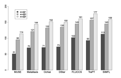
Figure 2: Comparison to other FL techniques: $acc@n$ metric values without counts of Closure

4.1.3 Comparison to Other FL Techniques

To gain some insights into the trade-off between amortised modelling efforts and localisation accuracy, we compare the method-level fault localisation results of the state-of-the-art MBFL and SBFL techniques, the result of which is shown in Figure 2. We obtained the performance of the each model (i.e., $acc@n$) on Defects4J from the literatures, and artefact of Zou et al. [35]. Based on the results of the comparison between SIMFL models, we choose MLP(F+P) to represent SIMFL. However, since Closure has been excluded from the evaluation of F+P models, we have excluded Closure from the results of other techniques for a fair comparison.

Figure 2 shows that MLP(F+P) is better than other techniques in terms of $acc@1$, but TraPT performs better in terms of $acc@3$ and $acc@5$. Although SIMFL does not make use of learning-to-rank technique to boost performance by fully including runtime information or suspiciousness scores of other FL techniques, SIMFL localises faults at the first rank better than others, and shows comparable results to the learning-to-rank techniques: FLUCCS and TraPT.

4.2 Model Viability on TEE (RQ2)

Table 6: Viability of F models using TEE scenario. The ranks that do not have the same ranks with FCE are typeset in bold.

Fault		Commit	Rank					Fault		Commit	Rank
		($\Delta$rev.)	EM	PM∗	PM+	LR	MLP			($\Delta$rev.)	EM	PM∗	PM+	LR	MLP
Closure	21	FCE Rank	2	2	2	2	2	Math	46	FCE Rank	188	188	188	47	85
		32a12ba (2)	2	2	2	2	2			bbb5e1e (1)	188	188	188	35	47
		43a5523 (3)	2	2	2	2	2			37680e2 (2)	188	188	188	35	47
	61	FCE Rank	7	4	5	5	6			1861674 (3)	188	188	188	35	27
		f5529dd (3)	7	4	5	5	6			f0b12de (4)	188	1	1	3	1
		b12d1d6 (4)	7	4	5	5	6			8581b76 (5)	188	188	188	35	41
		245362a (7)	7	4	5	5	7		89	FCE Rank	13	13	13	8	7
		8abd1d9 (8)	7	4	5	5	8			43336b0 (1)	12	12	12	2	3
		37b0e1b (9)	7	4	5	5	6			cdd62a0 (2)	14	14	14	2	5
	62	FCE Rank	1	1	1	1	1			90439e5 (3)	13	13	13	8	11
		245362a (2)	1	1	1	1	1			36a8485 (4)	13	13	13	8	13
		8abd1d9 (3)	1	1	1	1	1			dbe7842 (5)	13	13	13	8	7
		37b0e1b (4)	1	1	1	1	1			d84a587 (6)	13	13	13	8	12
	115	FCE Rank	14	22	24	19	11			d27e072 (7)	13	13	13	8	10
		b9262dc (5)	14	19	22	18	13			3590bdc (8)	13	13	13	8	8
		911b2d6 (6)	14	22	24	19	12			6b108c0 (9)	13	13	13	8	13
	120	FCE Rank	7	7	7	6	6			9c55428 (10)	13	13	13	8	12
		2aee36e (3)	24	24	24	15	16

Following the TEE scenario described in Section 3.1.2, we seek reference versions preceding the faulty version, i.e., the versions before the faulty version that pass all test cases of the fixed program, including the fault revealing test cases. Assuming that more recent versions are more likely to serve as references, given a faulty version $n$, we check $n-1$, …, $n-10$, $n-20$, and $n-30$ previous program versions, as it is impractical to inspect all of them. Starting from 357 faulty versions of subject programs, we found 28 preceding reference versions that correspond to seven different faulty versions. We have trained five F models on each of the 28 reference versions to localise the fault in the faulty version, resulting in 140 rankings based on TEE scenario. Note that we did not consider F+P models on these reference versions because they require more than 24 hours for mutation analysis, as described in Section 3.2.

Table 6 shows the rank of the faulty method for each F model built on each preceding reference version. Out of 140 TEE based rankings produced by F models, 103 are identical to the corresponding FCE ranking. One notable exception is Math 46 (f0b12de) that shows a significant improvement over the FCE scenario rank. We have manually examined the kill matrix of this reference version, and found that some mutants in the future faulty method have been additionally killed due to timeout (enforced by Major itself), contributing to the high rank (these mutants were not killed in other preceding reference versions of Math 46). We suspect that this is due to the non-determinism in the process of building the kill matrix: the mutation may have brought in flakiness that has been removed for the original program. We study the impact of different kill reasons in Section 5.3, and furthermore discuss this as one of the threats to internal validity in Section 6.

Note that, in all cases, the $\Delta$ revision values are ten or fewer, meaning that mutation analysis results from within ten past commits have been used to perform the localisation. Since the failing test cases in Defects4J are typically added against the buggy version, it is often impossible to execute it against a much older version of the same project, requiring a fairly recent kill matrix. We expect that, if the failing test case is an existing regression test that has remained executable for a long period of time, SIMFL will be more stable for longer durations. Our KMP scenario, which we will discuss in the next section, is also developed to cater for cases in which the mutation analysis results cannot be easily obtained for the failing test cases.

Table 7: Effectiveness of SIMFL models on KMP scenario, using all tests.

Model	Total	$acc@1$		$acc@3$		$acc@5$		$acc@10$
EM(F)	194	57	$-20$	95	$-44$	108	$-55$	122	$-82$
PM∗(F)	194	61	$-21$	101	$-50$	114	$-69$	131	$-94$
PM+(F)	194	60	$-26$	104	$-51$	119	$-67$	134	$-93$
LR(F)	194	63	$-27$	104	$-48$	116	$-70$	134	$-92$
MLP(F)	194	66	$-19$	106	$-44$	120	$-60$	140	$-83$
EM(F+P)	194	35	$-49$	57	$-51$	65	$-49$	82	$-37$
PM∗(F+P)	194	53	$+4$	76	$+2$	90	$+4$	107	$-3$
PM+(F+P)	194	66	$+33$	96	$+39$	119	$+51$	138	$+54$
LR(F+P)	194	96	$+8$	122	$+2$	133	$+4$	145	$+6$
MLP(F+P)	194	95	$-18$	125	$-20$	132	$-27$	150	$-31$
PC(F+P)	194	93	$-3$	132	$-11$	137	$-20$	148	$-30$

Table 8: Effectiveness of SIMFL models on KMP scenario, using relevant tests.

Model	Total	$acc@1$		$acc@3$		$acc@5$		$acc@10$
EM(F+P)	194	39	$-45$	64	$-44$	77	$-37$	94	$-25$
PM∗(F+P)	194	61	$+12$	91	$+17$	108	$+22$	131	$+21$
PM+(F+P)	194	66	$+33$	99	$+42$	114	$+46$	139	$+55$
LR(F+P)	194	63	$-25$	94	$-26$	112	$-17$	128	$-11$
MLP(F+P)	194	81	$-32$	109	$-36$	121	$-38$	143	$-38$
PC(F+P)	194	71	$-25$	109	$-34$	121	$-36$	137	$-41$

4.3 Localisation Effectiveness on KMP (RQ3)

We compute the scores of SIMFL models by following the KMP scenario that uses a predictive kill matrix by Seshat. Table 7 shows the aggregated numbers of each $acc@n$ metric as well as the difference with the results of the FCE scenario shown in Table 4. If the KMP scenario was better than the FCE scenario, we mark the differences with a plus sign, and if not, we mark them with a minus sign.

The most noticeable results in Table 7 is that, in case of some models, SIMFL with predicted kill matrices outperforms SIMFL with actual kill matrices. This seemingly counter-intuitive result is due to the way inaccurate predictions of Seshat affects SIMFL. Suppose Seshat predicts the kill matrix with the bias of more kills: this may result in an increased number of killed mutants in the faulty method, increasing its ranking score in turn. On the other hand, if Seshat predicts the kill matrix with the bias of fewer kills, it will result in the decreased number of killed mutants in the non-faulty methods, having a similar effect as that of passing test reducing the suspiciousness of the parts of the program they cover. Notably, this effect occurs strongly in partial models. In contrast, the performance of EM model degrades significantly. This is because, if SIMFL is to perform well, Seshat has to make a perfectly accurate prediction for the mutants in both the faulty method (to match F) and the non-faulty methods (to match P). Interestingly, the performance improvement from Seshat only applies to F+P models, suggesting that the support from P matches has a significant effect on the performance of SIMFL, as confirmed in RQ1. It is worth noting that MLP(F+P) model could not exhibit the best performance in terms of $acc@1$ metric, localising 18 fewer faults compared to the FCE scenario. This may be due to the superior capability of MLP model that can successfully learn the wrong predictions in the predicted kill matrix, which can result in a decrease in $acc@1$.

Note that, in RQ1, SIMFL uses only relevant tests as defined by Defects4J. However, the results in Table 7 is produced by predicting the entire kill matrices including all tests, meaning that SIMFL with Seshat has more information to localise faults. To investigate the impact of this difference, we also conducted the experiment for RQ3 by only predicting the kill matrix for relevant test cases using Seshat, the results of which are listed in Table 8. We can only use F+P models for this experiment, as the set of relevant tests includes both failing and passing tests. The $acc@n$ metrics produced with relevant tests are slightly degraded, but the overall trend remains the same: the performance of partial matching models either remains the same or slightly improved, but the performance of others degraded. Interestingly, the performance of EM(F+P) model is better when using relevant tests: since there are fewer tests to achieve exact match, it becomes easier to score high with EM(F+P) model.

Table 9: Uniform and stratified random sampling

Ratio	Model	Total	$acc$				N	$acc$
		Studied	@1	@3	@5	@10	(Ratio)	@1	@3	@5	@10
0.1	EM(F)	357	59.80	95.35	111.05	136.70	5 (0.27)	36.50	65.05	83.70	116.30
	PM∗(F)	357	66.55	107.85	126.55	159.35		40.95	74.75	94.95	133.20
	PM+(F)	357	68.40	108.50	128.50	162.25		40.05	75.00	97.25	134.20
	LR(F)	357	71.75	121.50	146.85	180.20		49.15	91.10	116.80	156.55
	MLP(F)	357	76.70	120.05	142.40	177.75		49.90	88.85	115.40	151.05
	EM(F+P)	224	46.35	56.55	62.10	70.75		39.50	57.05	64.20	69.10
	PM∗(F+P)	224	45.45	66.65	78.90	95.30		65.70	100.25	111.70	127.95
	PM+(F+P)	224	29.35	52.45	64.10	78.80		39.55	52.45	62.70	81.95
	LR(F+P)	224	70.70	93.30	104.30	117.10		75.95	114.40	128.30	146.05
	MLP(F+P)	224	83.60	111.30	122.10	139.60		78.15	118.20	134.50	152.00
	PC(F+P)	224	82.40	112.30	123.50	139.60		70.20	113.25	129.65	147.10
0.3	EM(F)	357	72.25	118.55	137.40	172.75	10 (0.41)	45.60	80.95	106.15	145.50
	PM∗(F)	357	78.90	132.15	156.25	196.20		49.65	93.50	122.15	161.40
	PM+(F)	357	83.45	133.70	159.40	200.40		53.65	93.00	120.20	162.60
	LR(F)	357	84.85	142.15	166.65	204.90		59.95	106.60	136.50	179.05
	MLP(F)	357	82.45	139.40	164.10	202.50		56.90	102.60	132.55	174.10
	EM(F+P)	224	66.70	82.35	89.25	95.40		50.60	74.00	80.85	85.50
	PM∗(F+P)	224	47.80	71.40	83.35	104.75		74.45	106.35	120.15	140.65
	PM+(F+P)	224	31.75	55.45	67.70	82.75		39.20	55.05	67.20	81.65
	LR(F+P)	224	81.95	107.60	116.40	131.50		82.15	115.90	128.80	146.70
	MLP(F+P)	224	101.55	132.20	143.40	159.85		89.70	126.35	141.60	161.45
	PC(F+P)	224	95.20	133.30	144.95	162.90		84.15	127.90	144.40	163.25
0.5	EM(F)	357	75.90	128.30	149.35	188.55	15 (0.50)	53.60	96.70	122.20	160.65
	PM∗(F)	357	82.90	141.80	168.85	211.15		58.70	110.10	139.65	177.95
	PM+(F)	357	86.30	143.80	173.60	215.20		62.20	109.15	142.75	182.70
	LR(F)	357	88.75	145.90	175.75	216.65		66.70	118.30	152.35	190.90
	MLP(F)	357	84.70	146.00	170.95	212.80		63.05	114.25	146.00	187.10
	EM(F+P)	224	73.90	93.10	100.05	106.50		57.35	82.65	89.45	94.75
	PM∗(F+P)	224	47.55	72.70	84.20	108.00		78.75	109.90	123.30	141.50
	PM+(F+P)	224	32.70	57.00	68.65	83.30		42.15	61.45	71.60	82.15
	LR(F+P)	224	86.35	112.15	121.75	135.20		86.95	116.95	129.70	148.35
	MLP(F+P)	224	104.90	138.65	151.35	166.70		94.80	134.60	147.95	163.60
	PC(F+P)	224	98.10	138.85	151.80	170.05		91.85	133.85	151.30	169.95
0.7	EM(F)	357	78.05	133.55	156.30	194.60	20 (0.56)	55.80	105.80	133.25	172.90
	PM∗(F)	357	84.80	147.75	175.60	216.90		64.95	121.45	153.75	193.75
	PM+(F)	357	88.15	150.05	177.85	219.30		70.05	124.10	156.30	195.10
	LR(F)	357	89.65	148.50	179.85	221.25		74.35	127.05	162.95	200.15
	MLP(F)	357	84.30	144.60	173.40	214.85		69.70	124.70	158.15	196.60
	EM(F+P)	224	78.05	98.85	106.05	112.15		62.50	88.05	94.05	100.55
	PM∗(F+P)	224	48.30	73.60	83.95	108.35		81.55	110.15	125.50	142.60
	PM+(F+P)	224	32.90	57.20	68.10	83.40		40.55	62.40	69.05	81.65
	LR(F+P)	224	87.20	115.20	125.15	137.85		90.70	118.60	131.60	148.90
	MLP(F+P)	224	108.45	142.55	155.30	170.20		98.25	138.20	150.00	165.90
	PC(F+P)	224	99.75	142.30	155.30	174.35		97.25	137.75	152.75	172.95
Full	EM(F)	357	77.00	139.00	164.00	204.00	Full	77.00	139.00	164.00	204.00
	PM∗(F)	357	82.00	151.00	183.00	224.00		82.00	151.00	183.00	224.00
	PM+(F)	357	86.00	155.00	186.00	227.00		86.00	155.00	186.00	227.00
	LR(F)	357	90.00	152.00	186.00	226.00		90.00	152.00	186.00	226.00
	MLP(F)	357	85.00	150.00	180.00	223.00		85.00	150.00	180.00	223.00
	EM(F+P)	224	84.00	108.00	114.00	119.00		84.00	108.00	114.00	119.00
	PM∗(F+P)	224	49.00	74.00	86.00	110.00		49.00	74.00	86.00	110.00
	PM+(F+P)	224	33.00	57.00	68.00	84.00		33.00	57.00	68.00	84.00
	LR(F+P)	224	88.00	120.00	129.00	139.00		88.00	120.00	129.00	139.00
	MLP(F+P)	224	113.00	145.00	159.00	181.00		113.00	145.00	159.00	181.00
	PC(F+P)	224	96.00	143.00	157.00	178.00		96.00	143.00	157.00	178.00

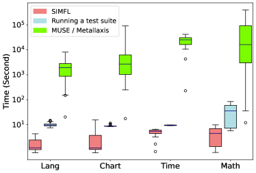
Figure 3: Execution time of SIMFL compared to MUSE, Metallaxis, and a full test suite run. Y-axis is shown on a logarithmic scale.

4.4 Efficiency (RQ4)

SIMFL is different from the other MBFL techniques in that it does not require test runs against the generated mutants after the fault is observed. Therefore, it may have an advantage over the existing MBFL techniques in terms of execution time and a faster feedback to the developers. To quantify this advantage, we compare the execution time of SIMFL with that of MUSE and Metallaxis, and a full test suite run. Note that we compare the online cost of SIMFL with other MBFL techniques that do not require generating a kill matrix in advance and hence have no offline cost. See Section 6 for the discussion on the online and offline costs of SIMFL.

To measure the execution time of SIMFL, we use the MLP model as it is the slowest model due to the training and inference time of it. As MUSE and Metallaxis lack open-source implementation, we employ a surrogate estimator to measure their execution time. That is, for each subject program, we collect the mutants covered by failing tests and measure the time for running the tests that cover them. Although MUSE and Metallaxis employ different formulae for calculating suspiciousness scores, we approximate their execution time to be the same because both require the same test runs to compute the scores (i.e., whether the mutants are killed or not) and the other computational costs are negligible compared to the test runs.

Figure 3 illustrates the execution time of running each technique, broken down by each project. Overall, SIMFL is on average 4.7x faster than running a full test suite and notably faster than MUSE and Metallaxis, showing on average 5,687x faster execution. The time gap between SIMFL and MUSE and Metallaxis is even larger for larger projects: SIMFL is on average 1,226x faster than MUSE and Metallaxis for the faults in Lang but 13,366x faster for the faults in Math. This result highlights the positive affect of the cost amortisation of SIMFL.

4.5 Effects of Sampling (RQ5)

To investigate how the mutation sampling rates affect the performance of SIMFL, we attempt to localise the studied faults using mutants sampled with different rates. Table 9 (left side) shows the uniform sampling results with rates of 0.1, 0.3, 0.5, and 0.7: all metric values are averaged across 20 different samples. Table 9 also includes the results obtained without sampling (Full). The best results are typeset in bold.

As expected, the Full configuration often shows the best performance, followed by sampling rates of 0.7 and 0.5. Since we expect different mutants to contribute different amounts of information to localisation, we do not find it surprising that sampling rates down to 0.5 show comparable results with the Full configuration. However, the performance does not degrade at the same rate as the sampling rate, as can be seen from the results obtained using the sampling rate of 0.1.

Since larger methods are likely to produce more mutants, uniform sampling will effectively sample more mutants for larger methods. We investigate whether this is disadvantageous for relatively smaller methods by evaluating stratified sampling: given the threshold parameter $N$, stratified sampling randomly chooses only $N$ mutants from methods with more than $N$ mutants, and chooses all mutants if their number is below $N$. Table 9 (right side) contains the results obtained using stratified mutant sampling with $N\in\{5,10,15,20\}$. The value in the parenthesis, i.e., “Ratio”, is the average ratio of the number of mutants sampled by stratified sampling to the number of all mutants.

Compared to the Full configuration, the performance degradation as $N$ decreases is notably worse than what has been observed from the results of uniform random sampling. However, even with $N=5$, the sample ratio is 0.27 on average, higher than the smallest sampling rate for the uniform sampling. The comparison suggests that, contrary to our concern for a potential bias against smaller methods, stratified sampling is actually harmful to SIMFL. One interpretation of the result is that, if we assume that the location of a fault is a random variable, larger methods are by definition more likely to contain it.

Table 10: The effects of removing subsumed mutants. For the results of each project, see Table LABEL:tab:dominance_extended.

Model	Total	$acc@1$		$acc@3$		$acc@5$		$acc@10$
EM(F)	357	92	$+15$	129	$-10$	144	$-19$	164	$-40$
PM∗(F)	357	126	$+44$	173	$+22$	191	$+8$	211	$-14$
PM+(F)	357	123	$+37$	170	$+15$	189	$+3$	208	$-19$
LR(F)	357	122	$+32$	170	$+18$	184	$-2$	216	$-10$
MLP(F)	357	136	$+51$	183	$+33$	206	$+26$	230	$+7$
EM(F+P)	224	75	$-9$	96	$-12$	106	$-8$	115	$-4$
PM∗(F+P)	224	71	$+22$	110	$+36$	123	$+37$	143	$+33$
PM+(F+P)	224	44	$+11$	91	$+34$	107	$+39$	139	$+55$
LR(F+P)	224	103	$+15$	134	$+14$	145	$+16$	156	$+17$
MLP(F+P)	224	119	$+6$	150	$+5$	157	$-2$	168	$-13$
PC(F+P)	224	102	$+6$	134	$-9$	145	$-12$	155	$-23$

4.6 Effects of Subsumed Mutants (RQ6)

It has been pointed out that mutation tools generate numerous subsumed and redundant mutants, resulting in a mutation score to be easily misunderstood [26, 27]. As the killing of the subsuming mutants always accompany the killing of their subsumed mutants, this problem not only inflates the mutation score but also inflate our method-level FL scores by SIMFL models. We investigate the effects of removing subsumed mutants. First, we identify the most subsuming mutants [36], which are located at the first rank of DMSG (Dynamic Mutant Subsumption Graph) [27] and are not subsumed by other mutants except their indistinguishable mutants. Next, we conduct RQ1 study using only subsuming mutants and compare $acc@n$ with the results of the original RQ1 study that uses all mutants.

As shown in Table 10, $acc@1$ of all models except EM(F+P) largely improved: MLP(F) localised 51 more faults at the first rank compared to the model using all mutants. The reason EM(F+P) worsened for all $acc@n$ is that the subsuming mutants are likely to be killed by a few tests and they eliminate subsumed mutants needed for exact matching. This reason also explains why the overall $acc@n$ of F models improved more than F+P models.

5 Discussion

5.1 Relation with Other FL Techniques

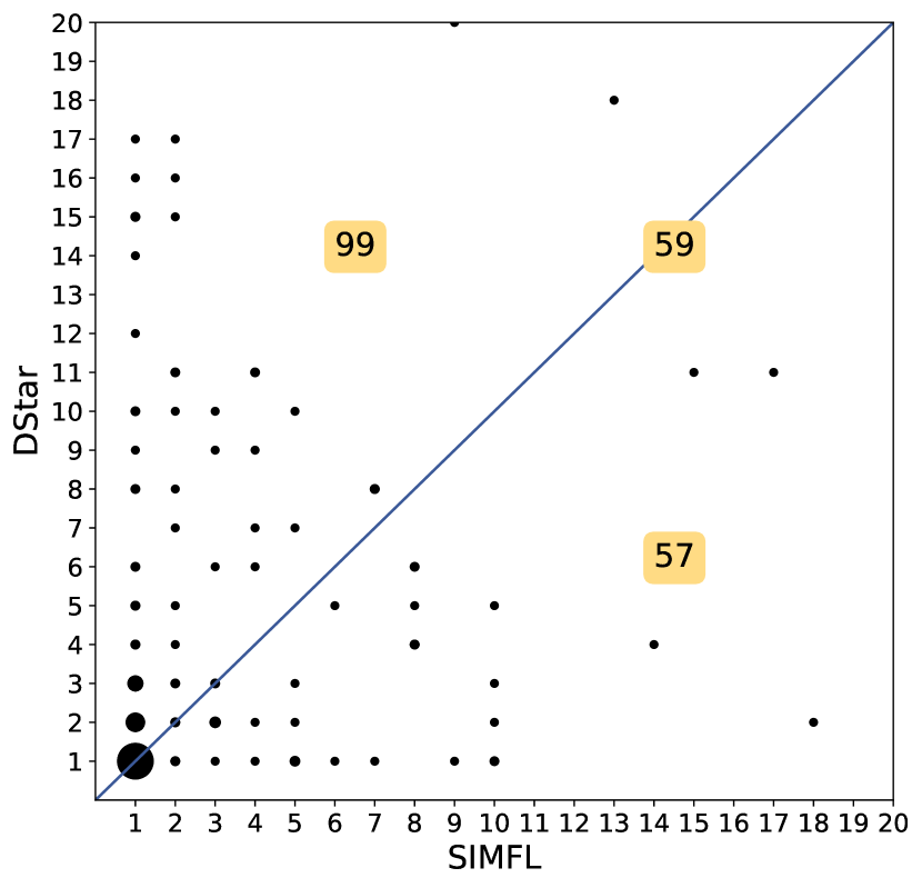
(a) DStar ($r=0.218$)

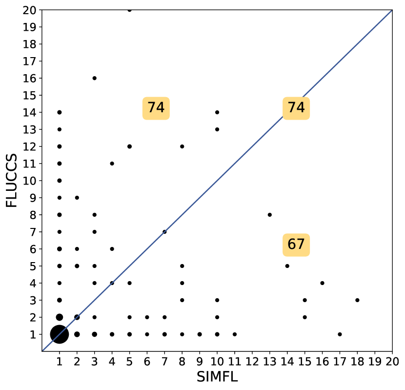
(b) FLUCCS ($r=0.105$)

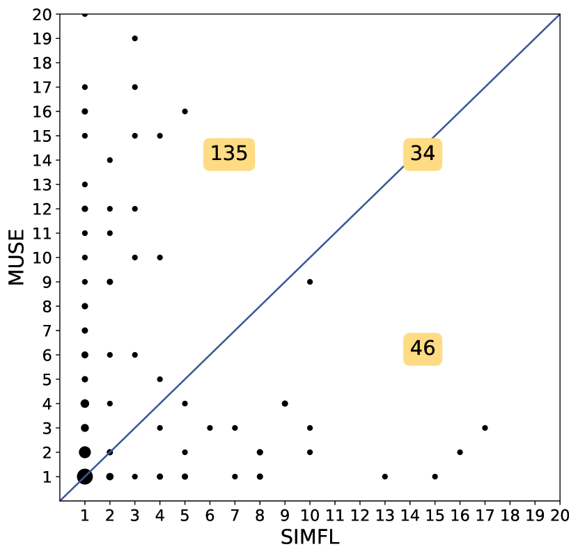
(c) MUSE ($r=0.072$)

(d) Metallaxis ($r=0.130$)

Figure 4: Comparison of MLP(F+P) and other FL techniques.

Two FL techniques can be complementary to each other if there is little overlap between faults ranked highly by each technique. To investigate whether the contribution of SIMFL is uniquely different from others, we investigate how individual faults are ranked differently by SIMFL and other FL techniques. SIMFL is represented by the MLP(F+P) model. We omit TraPT from this comparison as the individual rank information was not available from the paper.

Figure 4 plots each individual fault according to its rank by MLP(F+P) of SIMFL ($x$-axis) and its rank by the other FL technique ($y$-axis). Data points on the line $y=x$ represent faults that are ranked at the same place by both techniques, whereas the farther from the line a point is, the more differently it is ranked by two techniques. Plots only contain faults that are ranked within the top 20 places by at least one technique: the size of the dots corresponds to the number of faults plotted at the location of the dot. The numbers on the $y=x$ line as well as above and below the line show the total number of faults that belong to the corresponding parts, regardless of being ranked within the top 20 or not. For example, SIMFL ranks 135 faults higher than MUSE. The agreement between two techniques are measured using Pearson correlation coefficient ($r$): value 0 implies no correlation and, therefore, no agreement, whereas value 1 implies perfect correlation and, therefore, two identical rankings.

While there exist dense clusters of points near the top ranks around the $y=x$ line, there is no clear relationship between FL techniques. SIMFL shows low Pearson correlation coefficients against all compared techniques. Notably, SIMFL is significantly different from two existing MBFL techniques, MUSE and Metallaxis, suggesting that the way SIMFL captures the relationship between faults and tests differs significantly from existing MBFL techniques. SIMFL also ranks the most faults identically to FLUCCS, a technique that uses multiple SBFL scores as well as code and change metric, suggesting that mutation analysis can be a rich source of information for fault localisation. Overall, the results provide evidence that there exist faults that SIMFL can localise much more effectively than the other, and vice versa. The complementary nature also suggests the possibility of an effective hybridisation of SIMFL and other techniques, as recent work that combine multiple FL techniques suggest [35, 37, 2]. We leave the hybridisation as future work.

5.2 Test Case Granularity

Table 11: The result of Mann–Whitney U test on the number of methods whose mutants are killed by the failing test cases, between the faults localised within ($W3$) and out of top three places ($O3$). The significant level is 0.05: if $p$-value is less then 0.05 (typeset in bold), then we can reject null hypothesis that there is no significant difference between the two groups from which the samples were drawn.

Model	Project	$W3$			$O3$			$p$	Model	Project	$W3$			$O3$			$p$
		mean	std	sp	mean	std	sp				mean	std	sp	mean	std	sp
EM (F)	Lang	5.5	5.2	45	10.0	12.9	17	0.171	EM (F+P)	Lang	6.2	5.7	41	7.9	12.0	20	0.945
	Chart	10.0	6.8	11	144.9	260.5	15	0.002		Chart	11.4	7.3	9	136.1	254.5	16	0.017
	Time	69.2	36.1	9	129.6	46.7	17	0.003		Time	103.7	54.2	13	113.7	49.2	13	0.739
	Closure	167.2	117.3	31	322.7	182.2	101	0.000		Closure	-	-	-	-	-	-	-
	Math	15.5	19.1	43	34.8	26.6	59	0.000		Math	20.5	25.1	45	28.5	21.7	46	0.022
PM∗ (F)	Lang	5.1	3.8	47	11.9	14.3	15	0.125	PM∗ (F+P)	Lang	4.7	3.7	36	9.8	11.6	25	0.032
	Chart	10.0	6.8	11	144.9	260.5	15	0.002		Chart	96.3	242.1	9	88.4	193.4	16	0.074
	Time	78.4	43.9	10	127.6	47.4	16	0.013		Time	20.0	27.6	3	120.3	42.4	23	0.010
	Closure	175.7	113.8	36	327.6	184.9	96	0.000		Closure	-	-	-	-	-	-	-
	Math	15.4	18.8	47	36.3	26.6	55	0.000		Math	15.2	19.5	26	28.2	24.3	65	0.002
PM+ (F)	Lang	5.1	3.8	48	12.4	14.7	14	0.126	PM+ (F+P)	Lang	4.4	3.5	31	9.2	10.9	30	0.026
	Chart	9.8	7.1	10	136.6	254.3	16	0.004		Chart	96.9	242.0	9	88.1	193.5	16	0.106
	Time	78.4	43.9	10	127.6	47.4	16	0.013		Time	0.5	0.5	2	117.7	43.2	24	0.024
	Closure	203.2	160.8	41	323.5	178.0	91	0.000		Closure	-	-	-	-	-	-	-
	Math	15.5	19.1	46	35.8	26.5	56	0.000		Math	11.5	9.9	15	27.1	24.9	76	0.006
LR (F)	Lang	4.9	3.9	49	13.5	14.7	13	0.019	LR (F+P)	Lang	5.5	5.0	49	12.2	14.8	12	0.122
	Chart	11.8	6.2	9	135.9	254.6	16	0.019		Chart	70.3	200.9	14	117.9	223.1	11	0.118
	Time	78.4	43.9	10	127.6	47.4	16	0.013		Time	90.8	56.3	14	129.6	36.6	12	0.105
	Closure	193.3	136.7	37	322.3	184.0	95	0.000		Closure	-	-	-	-	-	-	-
	Math	16.5	19.1	47	35.3	27.1	55	0.000		Math	17.3	18.1	43	31.0	26.3	48	0.002
ML P(F)	Lang	5.4	5.1	51	12.9	15.0	11	0.042	MLP (F+P)	Lang	5.9	5.3	55	13.3	18.4	7	0.496
	Chart	10.8	6.6	10	144.9	260.5	15	0.004		Chart	14.6	10.1	13	174.2	283.7	12	0.019
	Time	62.3	40.0	10	137.7	34.7	16	0.000		Time	95.1	54.9	16	130.5	37.7	10	0.133
	Closure	168.6	114.0	33	325.3	183.0	99	0.000		Closure	-	-	-	-	-	-	-
	Math	15.6	18.9	46	35.8	26.7	56	0.000		Math	17.0	16.6	61	40.9	29.6	41	0.000
									PC (F+P)	Lang	5.4	4.0	51	12.7	16.5	11	0.592
										Chart	76.6	193.5	16	105.7	230.1	10	0.033
										Time	91.4	43.7	15	132.3	53.0	11	0.029
										Closure	-	-	-	-	-	-	-
										Math	16.5	17.4	61	41.8	28.1	41	0.000

A common pattern observed in all configurations of SIMFL is that it performs the best for Commons Lang. Following Laghari and Demeyer [38], we hypothesise that this may be related to the test case granularity: if each test case kills mutants that exist in only a few methods, SIMFL can benefit from this because failures of each test case will be tightly coupled with a few candidate locations.

To investigate the impact of test case granularity, we check whether the number of the methods that are relevant to failures caused by highly ranked faults is lower than the number of methods relevant to faults that are not ranked near the top. We define a method $m$ to be relevant to the failure of a test case $t$ if $t$ kills a mutant in $m$. A finer granularity test case $t$ is expected to be relevant to fewer methods. We categorise faults into those ranked in the top three places (set $W3$), and those that are not (set $O3$), and compare the number of relevant methods between $W3$ and $O3$.

Table 11 reports the results of Mann–Whitney U test on the number of relevant methods between $W3$ and $O3$. The column $sp$ shows the number of samples for each group and column $p$ shows the $p$-value. For 36 out of 49 cases, we accept the alternative hypothesis that there is a statistically significant difference between the number of relevant methods between $W3$ and $O3$. This supports our assumption that the faults in $W3$ are likely to be revealed by test cases with finer-granularity than the faults in $O3$. The test cases of Commons Lang have finer-granularity when compared to other subjects, leading us to conjecture that test case granularity is why SIMFL performs more effectively against Lang than others. However, the results also show that SIMFL is not simply reflecting a one-to-one mapping between methods (mutants) and their unit tests: failing test cases of Closure kill mutants in 203 methods on average, but PM⁺(F) can still localise 41 out of 132 faults within the top three places (see Table 4).

5.3 Kill Reason Filtering

Table 12: The $acc@n$ metric values after filtering mutants based on their kill reasons.

Model	Total	All			Assertion			Timeout			Exception
	Studied	$@1$	$@3$	$@5$	$@1$	$@3$	$@5$	$@1$	$@3$	$@5$	$@1$	$@3$	$@5$
EM(F)	357	77	139	163	100	163	179	21	30	38	53	90	107
PM∗(F)	357	82	151	183	108	185	206	23	35	44	60	97	117
PM+(F)	357	86	155	186	114	183	206	22	36	45	61	99	119
LR(F)	357	90	152	186	118	181	213	40	79	88	66	109	131
MLP(F)	357	85	150	180	121	189	210	43	76	91	60	106	129
EM(F+P)	224	84	108	114	72	89	96	7	11	16	55	64	68
PM∗(F+P)	224	49	74	86	50	76	90	23	42	57	49	71	80
PM+(F+P)	224	33	57	68	34	57	68	20	34	50	34	59	68
LR(F+P)	224	88	120	129	89	117	128	23	41	51	77	104	115
MLP(F+P)	224	113	145	159	112	147	160	29	50	55	91	120	135
PC(F+P)	224	96	143	157	100	145	160	22	36	43	78	113	121

A mutated program can cause a test failure due to many different reasons, such as assertion (i.e., test oracle) violation, uncaught exception, or timeout. All these reasons are normally marked as a kill. While all three reasons do reveal some dependency between the mutated location and the test outcome (otherwise the mutant would not be killed), we suspect that different kill reasons may have varying degrees of importance for fault localisation. Assertion violations would imply that the test oracles actually capture the correct program behaviour. Uncaught exceptions and timeouts, however, may only show coincidental impacts of the mutation.

Considering the relative importance of different kill reasons, we investigate whether filtering out the kill matrix based on the exact reason of test failure has any impact on the localisation effectiveness. This is partly motivated by the use of failure messages by TraPT [39]. We train SIMFL models using one of three kill reasons, and compare their results to those of models trained using all three reasons. Kill reasons supported by Major are: assertion violations (“Assertion”), timeouts (“Timeout”), and uncaught exceptions (“Exception”).

Table 12 shows the results of $acc@n$ metrics for SIMFL models of three different kill reasons. For all F models, using only mutants killed due to the assertion failures shows the best performance in terms of $acc@1$ and $acc@3$, adding support to our assumption that assertion violations reflect test oracles of correct program behaviour better than others. Timeouts appear to be the weakest signal.

However, for F+P models, the unfiltered original results (“All”) often show the best performance. This trend reveals a seemingly counter-intuitive, yet fundamental intuition about SIMFL: test cases in $\mathbf{T}_{f}$ and $\mathbf{T}_{p}$ contribute to localisation in different ways. If a test case $t$ is in $\mathbf{T}_{f}$, all mutants killed by $t$ earlier suggest that their locations may contain the fault. However, if $t\in\mathbf{T}_{p}$, all mutants killed by $t$ earlier suggests that their locations may not contain the fault that is detected by $t^{\prime}\in\mathbf{T}_{f}$. Consequently, kill reason filtering can make the contributions from tests in $\mathbf{T}_{f}$ more precise (i.e., to only reflect real fault detection), but may also reduce the total amount of contributions from tests in $\mathbf{T}_{p}$ because it removes potential locations that could have been excluded by being associated with a test in $\mathbf{T}_{p}$. This explains why, for F+P models, using only Assertion as the kill reason cannot dominate the results. Note that the distribution of kills between Assertion, Timeout, and Exception is likely not uniform, which we also think contributes to the mixed results of F+P models, combined with program semantics.

6 Threats to Validity

Given the controlled setting for our experiments and the clearly defined objective measures, there are few threats to the validity of our study. There are some threats to internal validity that are inherent to any mutation analysis and hard to completely avoid, such as non-determinism caused by mutation and equivalent mutants, which have been discussed in Section 4. Similarly, we see few threats to the construct and conclusion validity. The metrics we used are standard in the fault localisation literature. Additionally, we acknowledge that the small number of samples (sometimes less than 10) used in the Mann-Whitney U test may be a potential threat to the statistical power of our results.

Another potential threat to validity can arise from the offline costs of SIMFL. As SIMFL has to be ready for diverse future faults, it needs a larger kill matrix than other MBFL techniques that only need a partial kill matrix relevant to the fault. Therefore, if we compare these techniques within a single debugging scenario, SIMFL may be more expensive. Assuming that the cost of running the test suite is the same for all mutants, then we can estimate the offline costs by comparing the number of mutants that need to be executed against the test suite. In our analysis on the subject programs, the ratio between the mutants that are relevant to a single fault on average and the total number of mutants is approximately 1 to 6. This means that after localising about 6 faults, performing a full-scale mutation analysis in advance can result in a more usable MBFL technique than analyzing mutations for each test failure, as it allows for parallelisation and offline execution. Additionally, reducing the offline costs of SIMFL can be achieved by creating a partial kill matrix for program elements more likely to have faults based on defect prediction strategies.

As suggested by Steimann et al. [40], the presence of multiple faults can be the threat to validity. This can complicate the fault localization process and lead to less accurate results. In practice, it is not always possible to achieve perfect bug detection, resulting in increased effort required to detect faults. Additionally, we should note that our assumption that a failing test case executes at least one faulty position in the source code may introduce a potential bias and influence the validity of our results.

Rather, the main threat of our study is to its external validity. Even though we studied five different subjects from the real-world Defects4J benchmark to mitigate this threat, this does not allow us to generalise to many, other programs and test suite contexts. Still, there was enough variation among the subjects for us to identify SIMFL’s dependence on the granularity of the test cases.

7 Related Work

7.1 Mutation-based Fault Localisation

A number of MBFL techniques have been proposed in the literature. Metallaxis uses SBFL-like formulas to measure the similarity between failure patterns of the actual fault and mutants [13, 12]. MUSE [10], and its variation MUSEUM [11], depend on two principles: first, if we mutate already faulty parts of the program, it is unlikely that we will observe more failing test cases, and we may even observe partial fixes, and second, if we mutate non-faulty parts, tests that used to pass are now likely to fail. MUSE and MUSEUM define their suspiciousness scores using the ratios of fail-become-pass and pass-become-fail tests. TraPT is similar to MUSE and MUSEUM in nature, but transforms both the output messages of failing tests, to distinguish different types of exceptions, and the test code itself, to prevent early program termination due to the assertion violation that precludes collecting information of other assertions  [39].

MBFL techniques suffer from the cost of mutation analysis, as it requires a massive number of test executions against the generated mutants. To reduce the number of mutants needed to be inspected, Metallaxis [13] adopts mutant sampling while HOTFUZ [18] combines first-order mutants to build higher-order mutants and computes suspicious score only on them. Their results showed that this reduces the number of total mutants as well as equivalent mutants that contribute nothing to the fault localisation. Despite such efforts to reduce the costs, all existing MBFL techniques inevitably mutate the faulty program and execute tests once testing is finished. In contrast, SIMFL allows the mutation analysis to be performed ahead of time.

7.2 Deep Learning Based Fault Localisation

DeepFL [41] is a Deep Learning (DL) based learning-to-rank FL technique that integrates the results of multiple FL techniques. By aggregating a variety of information such as program spectrum, mutation, and source code metrics, they achieve better FL performance than the individual techniques. On the other hand, DEEPRL4FL [42] leverages a coverage matrix, a data flow graph, and abstract syntax trees to learn to localise the faults, using Convolutional Neural Networks (CNNs). Both techniques have shown promising results through utilising multiple sources of information. In contrast, SIMFL stands out as a single MBFL technique that is orthogonal to the existing MBFL techniques, presenting a potential opportunity for integration as a distinctive feature in the synthesis of FL results.

7.3 Bayesian Inference for Fault Localisation

SIMFL was initially formulated based on Bayesian analysis to infer likely fault locations given test information. In the context of fault localisation, Abreau et al. [43] have introduced Barinel, a SBFL technique that adopts Bayesian reasoning to generate candidate sets of multiple fault locations. To the best of our knowledge, SIMFL is the first MBFL technique that uses Bayesian inference as well as other statistical inference techniques. While SIMFL also uses dynamic information from mutation, the mutation analysis can be performed ahead of time, which allows the cost to be amortised over multiple development iterations, and provides faster feedback.

7.4 Mutant Subsumption

The subsumption relationship between two mutants appears when both are killed by the tests and all tests that kill the one also kill the other. Therefore, this indicates a redundancy of the subsumed mutant [32], allowing the mutation score to be inflated. As a result, building a minimal set of mutants can enhance the validity and efficacy of mutation analysis [27]. We showed that SIMFL can exploit this by removing the subsumed mutants in the kill matrix and achieve considerably better results than the normal setting using all mutants.

7.5 Predictive Mutation Testing

A recent advance to deal with the high costs of mutation testing is Predictive Mutation Testing (PMT) [21, 22]. PMT predicts the mutation score as well as test results of each mutant. Since PMT uses historical mutation testing results as its features to train the predictive model, PMT and SIMFL have a similar scenario that amortises the cost of mutation testing. However, PMT is originally designed to predict whether a test suite can kill the mutants, so it is hard to apply to SIMFL that requires the test-case level results of mutant kills. Seshat [23] provides a test-case level prediction of mutant kills using the tokens in the source code and test as well as the dynamic information of the mutants. The finer-grained prediction of Seshat enables its combined use with SIMFL, which helps SIMFL to deal with newly introduced test cases by simply predicting which mutants they can kill.

8 Conclusion

In this paper, we introduce SIMFL, a Mutation Based Fault Localisation (MBFL) technique utilising mutation analysis results of the earlier version. SIMFL models the relations between the location of the artificial faults (i.e., mutants) and their test results via several modelling schemes such as statistical inference or machine learning techniques. After the faults are observed, SIMFL infers their locations without any mutant executions. We evaluate SIMFL on the real-faults in Defects4J dataset and the results show that SIMFL can locate 113 faults on the first rank out of 224 faults. Even if we simulate SIMFL on the predicted kill matrix, SIMFL still localises 95 faults on the first rank out of 194 faults, supporting its practical applicability. Moreover, we demonstrate that removing the subsumed mutants significantly improves the localisation accuracy of SIMFL.

References

- [1] S. Yoo, Evolving human competitive spectra-based fault localisation techniques, in: G. Fraser, J. Teixeira de Souza (Eds.), Search Based Software Engineering, Vol. 7515 of Lecture Notes in Computer Science, Springer Berlin Heidelberg, 2012, pp. 244–258.
- [2] J. Sohn, S. Yoo, Fluccs: Using code and change metrics to improve fault localisation, in: Proceedings of the International Symposium on Software Testing and Analysis, ISSTA 2017, 2017, pp. 273–283.
- [3] R. Abreu, P. Zoeteweij, A. J. C. van Gemund, Simultaneous debugging of software faults, J. Syst. Softw. 84 (4) (2011) 573–586.
- [4] L. Naish, H. J. Lee, K. Ramamohanarao, A model for spectra-based software diagnosis, ACM Transactions on Software Engineering Methodology 20 (3) (2011) 11:1–11:32.
- [5] S. Yoo, X. Xie, F.-C. Kuo, T. Y. Chen, M. Harman, Human competitiveness of genetic programming in sbfl: Theoretical and empirical analysis, ACM Transactions on Software Engineering and Methodology 26 (1) (2017) 4:1–4:30.
- [6] W. E. Wong, Y. Qi, L. Zhao, K.-Y. Cai, Effective fault localization using code coverage, in: Proceedings of the 31st Annual International Computer Software and Applications Conference - Volume 01, COMPSAC ’07, IEEE Computer Society, Washington, DC, USA, 2007, pp. 449–456. doi:10.1109/COMPSAC.2007.109.
- [7] Y. Qi, X. Mao, Y. Lei, C. Wang, Using automated program repair for evaluating the effectiveness of fault localization techniques, in: Proceedings of the 2013 International Symposium on Software Testing and Analysis, ISSTA 2013, ACM, New York, NY, USA, 2013, pp. 191–201. doi:10.1145/2483760.2483785.
- [8] W. Weimer, T. Nguyen, C. L. Goues, S. Forrest, Automatically finding patches using genetic programming, in: Proceedings of the 31st IEEE International Conference on Software Engineering (ICSE ’09), IEEE, Vancouver, Canada, 2009, pp. 364–374.
-
[9]
M. Wen, J. Chen, R. Wu, D. Hao, S.-C. Cheung,
Context-aware patch
generation for better automated program repair, in: Proceedings of the 40th
International Conference on Software Engineering, ICSE ’18, ACM, New York,
NY, USA, 2018, pp. 1–11.
doi:10.1145/3180155.3180233.
URL http://doi.acm.org/10.1145/3180155.3180233 - [10] S. Moon, Y. Kim, M. Kim, S. Yoo, Ask the mutants: Mutating faulty programs for fault localization, in: Proceedings of the 7th International Conference on Software Testing, Verification and Validation, ICST 2014, 2014, pp. 153–162.
- [11] S. Hong, T. Kwak, B. Lee, Y. Jeon, B. Ko, Y. Kim, M. Kim, Museum: Debugging real-world multilingual programs using mutation analysis, Information and Software Technology 82 (2017) 80–95.
- [12] M. Papadakis, Y. Le-Traon, Using mutants to locate ”unknown” faults, in: Proceedings of the 5th IEEE Fifth International Conference on Software Testing, Verification and Validation, Mutation 2012, 2012, pp. 691–700. doi:10.1109/ICST.2012.159.
-
[13]
M. Papadakis, Y. L. Traon,
Metallaxis-fl: mutation-based
fault localization, Softw. Test., Verif. Reliab. 25 (5-7) (2015) 605–628.
doi:10.1002/stvr.1509.
URL http://dx.doi.org/10.1002/stvr.1509 -
[14]
S. Pearson, J. Campos, R. Just, G. Fraser, R. Abreu, M. D. Ernst, D. Pang,
B. Keller, Evaluating and
improving fault localization, in: Proceedings of the 39th International
Conference on Software Engineering, ICSE ’17, IEEE Press, Piscataway, NJ,
USA, 2017, pp. 609–620.
doi:10.1109/ICSE.2017.62.
URL https://doi.org/10.1109/ICSE.2017.62 - [15] A. J. Offutt, Investigations of the software testing coupling effect, ACM Transactions on Software Engineering Methodology 1 (1992) 3–18.
-
[16]
R. Just, D. Jalali, L. Inozemtseva, M. D. Ernst, R. Holmes, G. Fraser,
Are mutants a valid
substitute for real faults in software testing?, in: Proceedings of the 22Nd
ACM SIGSOFT International Symposium on Foundations of Software Engineering,
FSE 2014, ACM, New York, NY, USA, 2014, pp. 654–665.
doi:10.1145/2635868.2635929.
URL http://doi.acm.org/10.1145/2635868.2635929 - [17] Y. T. Chen, R. Gopinath, A. Tadakamalla, M. D. Ernst, R. Holmes, G. Fraser, P. Ammann, R. Just, Revisiting the relationship between fault detection, test adequacy criteria, and test set size, in: Proceedings of the 35th IEEE/ACM International Conference on Automated Software Engineering, 2020, pp. 237–249.
- [18] J.-I. Jang, D. Ryu, J. Baik, Hotfuz: Cost-effective higher-order mutation-based fault localization, Software Testing, Verification and Reliability (2021) e1802.
- [19] G. Petrović, M. Ivanković, G. Fraser, R. Just, Does mutation testing improve testing practices?, in: 2021 IEEE/ACM 43rd International Conference on Software Engineering (ICSE), IEEE, 2021, pp. 910–921.
- [20] M. Meyer, Continuous integration and its tools, IEEE software 31 (3) (2014) 14–16.
- [21] J. Zhang, L. Zhang, M. Harman, D. Hao, Y. Jia, L. Zhang, Predictive mutation testing, IEEE Transactions on Software Engineering 45 (9) (2018) 898–918.
- [22] D. Mao, L. Chen, L. Zhang, An extensive study on cross-project predictive mutation testing, in: 2019 12th IEEE Conference on Software Testing, Validation and Verification (ICST), IEEE, 2019, pp. 160–171.
- [23] J. Kim, J. Jeon, S. Hong, S. Yoo, Predictive mutation analysis via natural language channel in source code, ACM Trans. Softw. Eng. Methodol.
- [24] R. Just, D. Jalali, M. D. Ernst, Defects4j: A database of existing faults to enable controlled testing studies for java programs, in: Proceedings of the 2014 International Symposium on Software Testing and Analysis, ISSTA 2014, ACM, New York, NY, USA, 2014, pp. 437–440. doi:10.1145/2610384.2628055.
- [25] R. Just, F. Schweiggert, G. M. Kapfhammer, Major: An efficient and extensible tool for mutation analysis in a java compiler, in: 2011 26th IEEE/ACM International Conference on Automated Software Engineering (ASE 2011), 2011, pp. 612–615. doi:10.1109/ASE.2011.6100138.
- [26] R. Just, G. M. Kapfhammer, F. Schweiggert, Do redundant mutants affect the effectiveness and efficiency of mutation analysis?, in: 2012 IEEE Fifth International Conference on Software Testing, Verification and Validation, IEEE, 2012, pp. 720–725.
- [27] P. Ammann, M. E. Delamaro, J. Offutt, Establishing theoretical minimal sets of mutants, in: 2014 IEEE seventh international conference on software testing, verification and validation, IEEE, 2014, pp. 21–30.
- [28] J. Kim, G. An, R. Feldt, S. Yoo, Ahead of time mutation based fault localisation using statistical inference, in: 2021 IEEE 32nd International Symposium on Software Reliability Engineering (ISSRE), 2021, pp. 253–263. doi:10.1109/ISSRE52982.2021.00036.
- [29] P. S. Kochhar, X. Xia, D. Lo, S. Li, Practitioners’ expectations on automated fault localization, in: Proceedings of the 25th International Symposium on Software Testing and Analysis, ISSTA 2016, ACM, New York, NY, USA, 2016, pp. 165–176.
- [30] H.-F. Yu, F.-L. Huang, C.-J. Lin, Dual coordinate descent methods for logistic regression and maximum entropy models, Machine Learning 85 (1-2) (2011) 41–75.
- [31] G. E. Hinton, Connectionist learning procedures, in: Machine learning, Elsevier, 1990, pp. 555–610.
- [32] B. Kurtz, P. Ammann, M. E. Delamaro, J. Offutt, L. Deng, Mutant subsumption graphs, in: 2014 IEEE Seventh International Conference on Software Testing, Verification and Validation Workshops, IEEE, 2014, pp. 176–185.
-
[33]
J. Liang, S. Elbaum, G. Rothermel,
Redefining prioritization:
Continuous prioritization for continuous integration, in: Proceedings of the
40th International Conference on Software Engineering, ICSE ’18, ACM, New
York, NY, USA, 2018, pp. 688–698.
doi:10.1145/3180155.3180213.
URL http://doi.acm.org/10.1145/3180155.3180213 - [34] S. Shamshiri, R. Just, J. M. Rojas, G. Fraser, P. McMinn, A. Arcuri, Do automatically generated unit tests find real faults? an empirical study of effectiveness and challenges, in: 2015 30th IEEE/ACM International Conference on Automated Software Engineering (ASE), 2015, pp. 201–211. doi:10.1109/ASE.2015.86.
- [35] D. Zou, J. Liang, Y. Xiong, M. D. Ernst, L. Zhang, An empirical study of fault localization families and their combinations, IEEE Transactions on Software Engineering.
- [36] M. Papadakis, C. Henard, M. Harman, Y. Jia, Y. Le Traon, Threats to the validity of mutation-based test assessment, in: Proceedings of the 25th International Symposium on Software Testing and Analysis, 2016, pp. 354–365.
- [37] J. Xuan, M. Monperrus, Learning to combine multiple ranking metrics for fault localization, in: Proceedings of the IEEE International Conference on Software Maintenance and Evolution, ICSME 2014, 2014, pp. 191–200. doi:10.1109/ICSME.2014.41.
-
[38]
G. Laghari, S. Demeyer, Unit
tests and component tests do make a difference on fault localisation
effectiveness, in: Proceedings of the 40th International Conference on
Software Engineering: Companion Proceeedings, ICSE ’18, ACM, New York, NY,
USA, 2018, pp. 280–281.
doi:10.1145/3183440.3194970.
URL http://doi.acm.org/10.1145/3183440.3194970 - [39] X. Li, L. Zhang, Transforming programs and tests in tandem for fault localization, Proceedings of the ACM on Programming Languages 1 (OOPSLA) (2017) 92.
- [40] F. Steimann, M. Frenkel, R. Abreu, Threats to the validity and value of empirical assessments of the accuracy of coverage-based fault locators, in: Proceedings of the 2013 International Symposium on Software Testing and Analysis, ISSTA 2013, ACM, New York, NY, USA, 2013, pp. 314–324.
- [41] X. Li, W. Li, Y. Zhang, L. Zhang, Deepfl: Integrating multiple fault diagnosis dimensions for deep fault localization, in: Proceedings of the 28th ACM SIGSOFT international symposium on software testing and analysis, 2019, pp. 169–180.
- [42] Y. Li, S. Wang, T. Nguyen, Fault localization with code coverage representation learning, in: 2021 IEEE/ACM 43rd International Conference on Software Engineering (ICSE), IEEE, 2021, pp. 661–673.
- [43] R. Abreu, P. Zoeteweij, A. van Gemund, Spectrum-based multiple fault localization, in: Proceedings of the 24th IEEE/ACM International Conference on Automated Software Engineering, ASE 2009, 2009, pp. 88–99. doi:10.1109/ASE.2009.25.