Proteus: Simulating the Performance of
Distributed DNN Training

Abstract

DNN models are becoming increasingly larger to achieve unprecedented accuracy, and the accompanying increased computation and memory requirements necessitate the employment of massive clusters and elaborate parallelization strategies to accelerate DNN training. In order to better optimize the performance and analyze the cost, it is indispensable to model the training throughput of distributed DNN training. However, complex parallelization strategies and the resulting complex runtime behaviors make it challenging to construct an accurate performance model. In this paper, we present Proteus, the first standalone simulator to model the performance of complex parallelization strategies through simulation execution. Proteus first models complex parallelization strategies with a unified representation named Strategy Tree. Then, it compiles the strategy tree into a distributed execution graph and simulates the complex runtime behaviors, comp-comm overlap and bandwidth sharing, with a Hierarchical Topo-Aware Executor (HTAE). We finally evaluate Proteus across a wide variety of DNNs on three hardware configurations. Experimental results show that Proteus achieves $3.0\%$ average prediction error and preserves order for training throughput of various parallelization strategies. Compared to state-of-the-art approaches, Proteus reduces prediction error by up to $133.8\%$.

I Introduction

Recent years, progressively larger DNN models continue to break predictive accuracy records [1, 2, 3, 4, 5, 6, 7]. As these models grow, they are becoming computationally and memory expensive to train. To efficiently train DNN models, large GPU clusters and sophisticated parallelization strategies are employed to accelerate the training process [8, 9, 10, 11, 12, 13, 14, 15, 16]. For example, NVIDIA trained an 8.3 billion parameters language model on 512 GPUs with expert-designed hybrid data and model parallelism [10].

Since the training performance (throughput) of a DNN highly depends on its parallelization strategy, a natural question to ask is that can we accurately model the performance of any parallelization strategy for a specified cluster. Modeling the performance of a parallelization strategy is crucial for performance optimization and analysis. 1) Knowing the performance of a parallelization strategy can guide our optimization. Performance model can be leveraged to locate the bottleneck of a parallelization strategy in manual optimization and compare different parallelization strategies in automated parallelization systems [17, 18, 19, 20]. 2) Because implementing a parallelization strategy on current deep learning frameworks [21, 22] is error-prone, labor-intensive and resource-costing, an accurate performance model can save lots of effort and resources in evaluating it. 3) Predicting the performance of a parallelization strategy in advance can help us analyze cloud service budgets without requiring GPU resources, such as how many machine hours or nodes to buy, thereby saving computing resources.

Plenty of performance modeling approaches have been proposed to predict the performance of DNN models, but none of them scale beyond hybrid data and model parallelism. Most of recent efforts to model the performance of DNN models are constrained to the scenario of single GPU. For example, various analytical models [23, 24, 25] that build with hardware metrics and learning-based models [26, 27] that learn from runtime statistics are presented to study the performance of GPU kernels. In multi-GPU scenario, prior works [28, 29, 30] build analytical or profiling-based performance models for different DNN layers and predict training performance by summing up the computation and communication time of each layer. These approaches focus on a small subset of parallelization strategies and are not applicable to emerging parallelization strategies.

Some automated parallelization approaches [19, 17, 31] also build performance models for distributed DNN training. For example, FlexFlow [17] customizes a simulator to evaluate parallelization strategies in SOAP space. However, these works aim at searching optimal parallelization strategy for a DNN model instead of accurate performance modeling for general parallelization strategies. The usability and scalability are greatly limited due to their non-programmability of parallelization strategy and small strategy space.

We find two main challenges that hinder us from constructing accurate performance models for distributed DNN training. One challenge is how to model complex parallelization strategies. Since different parallelization strategies own distinct computation and memory consumption characteristics, handcrafted strategies that are composed of various parallelization strategies at diferent levels are designed to accelerate DNN training, especially large DNN models [10, 11, 12, 13, 14, 15, 16]. For example, Megatron-LM combines recomputation [32] and hybrid pipeline, data and model parallelism to train large transformer models [10]. The other challenge is how to model complex runtime behaviors. The underlying assumption of prior works [29, 30, 31, 17] is that the cost of a single operator only depends on its input and output tensor shape and it does not hold when meeting complex parallelization strategies. During runtime, communication operators can be overlapped with computation operators to hide the cost of gradient synchronization, and communication operators in different communication groups may share bandwidth resources. Such optimization or sharing is not free but will increase the cost of these operators and thus decreasing the throughput of the entire DNN model. Therefore, an accurate performance model should be able to explicitly capture the optimizations of complex parallelization strategies and the overhead incurred due to complex runtime behaviors.

TABLE I: Comparison of Proteus and existing approaches. Approaches in italics are automated parallelization frameworks, the others are performance modeling frameworks.

Approach	Complex Parallelization Strategy				Complex
	Operator-Level		Subgraph-Level		Runtime
	Comp.	Mem.	Pipeline	Recomp.	Behavior
DAPPLE [19]	Data		✓
FlexFlow [17]	SOAP
Yan et al. [29]	Hybrid
Pei et al. [28]	Data
Paleo [30]	Hybrid
Proteus (ours)	Shard	✓	✓	✓	✓

To address these challenges, we present Proteus, a standalone simulation framework that aims at accurately modeling the training throughput for distributed DNN training. Table I highlights the advantages of Proteus against existing approaches.

First, we introduce a hierarchical tree structure, Strategy Tree, to model complex parallelization strategies. We find parallelization strategies can be classified into operator- and subgraph-level strategies as a DNN graph is often divided into disjoint subgraphs, each of which is assigned to a group of devices. The strategies at operator-level specify how the operators and tensors are split and mapped to devices, while the strategies at subgraph-level indicate how to schedule subgraphs (details refer to Section II). The hierarchical structure of strategy tree provides a unified representation for parallelization strategies at different levels and enables Proteus to model the huge and complex strategy space.

Second, we propose HTAE (Hierarchical Topo-Aware Executor) to simulate complex runtime behaviors, which are ignored in prior works. We observe that runtime behaviors that have a significant impact on performance can be categorized into two types, comp-comm overlap and bandwidth sharing. HTAE simulates the schedule of subgraphs and operators to detect runtime behaviors during execution and adapts operator cost according to detailed cluster topology, thus capturing complex runtime behaviors of different operators.

Given a DNN model and Strategy Tree, Proteus automatically compiles them into a distributed execution graph by splitting operators and tensors and inserting inferred collective communication operators. Afterwards, Proteus predicts the training throughput and OOM (Out-Of-Memory) error by mimicking the schedule and execution of the execution graph considering the cluster topology.

In summary, we propose Proteus, to the best of our knowledge, the first standalone simulator to enable simulating complex parallelization strategies through fine-grained scheduling and simulation execution. We make the following contributions in building Proteus:

1. We classify parallelization strategies into operator- and subgraph-level and formulate a unified parallelization space with Strategy Tree to model complex parallelization strategies.

2. We identify two types of runtime behaviors that affect performance: comp-comm overlap and bandwidth sharing, and introduce Hierarchical Topo-Aware Executor to dynamically detect and model such behaviors.

3. We evaluate Proteus across a wide variety of DNNs on 3 hardware configurations. Experiments show that Proteus achieves $3.0\%$ average prediction error and preserves order for training throughput of various parallelization strategies. Compared to state-of-the-art approaches, Proteus reduces prediction error by up to $133.8\%$.

II Background: Distributed DNN training

DNNs are commonly represented as computation graphs in modern DL frameworks [21, 22], with nodes as operators and edges as tensors. Parallelizing a DNN involves parallelizing elements in the computation graph which can be categorized into two levels of parallelization strategies.

Operator-Level Strategy

Operators and tensors can be partitioned for parallel execution on multiple devices. This partitioning is operator-level, which can be further categorized into computation parallelization and memory optimization based on corresponding computation and memory aspects.

Computation Parallelization is achieved by partitioning the parallelizable dimensions of operators. Typically, we consider every unique dimension occurred in input or output tensors as parallelizable dimensions. We will describe different parallelization strategies taking the linear operator in Figure 1a as an example: $output(b,s,o)=\sum_{h}input(b,s,h)\times weight(o,h)$. There are 4 unique dimensions: $b(batch)$, $s(sequence)$, $o(output\_channel)$, $h(hidden/reduction)$.

Data parallelism is the most widely used parallelization strategy, which splits batch dimension ($b$) and replicates $weight$ on all devices.

Model parallelism divides the operator in $o$ or $h$ dimension thus partitioning $weight$ into different parts and each part is trained on a dedicated device.

Hybrid parallelism combines both data and model parallelism to partition operators.

Op shard is a general parallelization strategy that exploits the power of partitioning arbitrary dimensions of ($b,s,o,h$).

Figure 1a shows an example configuration to shard an operator in $b$ and $h$ dimensions. The partition describes how to parallelize different dimensions and map specifies how to place each partition. The operator is split into 4 ($|$partition$|$) parts, with each assigned to a GPU. As reduction dimension ($h$) is partitioned, the operator produces 4 partial output tensors, which should be aggregated to produce the final output tensor.

In this paper, Proteus targets on modeling the performance of general op shard unlike prior works that focus on data and model parallelism [28, 30, 29]. SOAP [17] partitions operators in $b,s,o$ dimensions and is a sub-space of op shard.

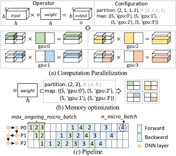
Figure 1: Examples of parallelization strategies.

Memory Optimization. All dimensions of a tensor are parallelizable. Partitioning a tensor is achieved by splitting along its dimensions similar to partitioning operators.

ZeRO [13] and Activation partitioning [33] partitions tensors in the first dimension and maps each part to a device to reduce redundancy. They can be combined with parallelization in other dimensions. Figure 1b shows an example that partitions $o$ (ZeRO) and $h$ dimensions.

Proteus explicitly defines a parallelization strategy for each tensor in a DNN model. Figure 1a shows that splitting an operator also creates implicit parallelization strategy for its input and output tensors. The inconsistency between the implicit and explicit strategy will incur additional communication (e.g. weight need to transform from strategy of Figure 1b to the implicit strategy of Figure 1a).

Subgraph-Level Strategy

A subgraph is composed of operators and tensors with dependencies. Parallelization strategies that describe the schedule of subgraphs are called subgraph-level strategies, including pipeline parallelism and recomputation, which balance training throughput and memory footprint by parallelizing subgraph computations.

Pipeline parallelism divides a computation graph into disjoint parts and assigns each part to a device group. It splits a batch input data into multiple micro-batches to exploit parallelism [34]. Figure 1c shows a pipeline example with n_micro_batch micro-batches for each subgraph. To reduce memory consumption, forward and backward micro-batches are interleaved [20], and max_ongoing_micro_batch limits the number of forward micro-batches on the flight.

Recomputation (Activation Checkpointing) [32] is a schedule that trades computation for memory. It frees forward subgraph activations after execution and recomputes when intermediate activations are required in backward pass.

Parallelization strategies at operator- and subgraph-level can be incorporated together thus formulating a complex parallelization space. Proteus leverages the hierarchical property to model complex parallelization strategies.

III Proteus Overview

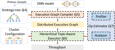
Figure 2: An Overview of Proteus.

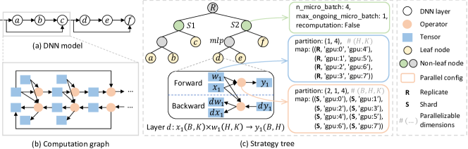
Figure 3: (a) A DNN model with 6 layers. (b) The computation graph of (a), including forward and backward computations. (c) The strategy tree of (a). Parallel configurations are assigned to non-leaf nodes and leaf nodes.

Figure 2 shows an overview of Proteus, a simulation framework towards accurate performance modeling for distributed DNN training. Since the performance of distributed DNN training highly depends on the parallelization strategy, explicitly modeling a parallelization strategy is the first step for a performance model. Proteus uses a unified representation strategy tree to model complex parallelization strategies (Section IV).

Proteus’s execution graph compiler (Section V) bridges the gap between high level parallelization strategy and low level execution. It takes DNN model and strategy tree as inputs, and compiles DNN layers into tensors and operators. The compiler automatically inserts communication operators between tensors and generates a distributed execution graph.

In Section VI, we first discuss the characterization and impact of runtime behaviors, then introduce Proteus’s hierarchical topo-aware executor, which simulates the schedule of the execution graph and predicts the training throughput. During simulation, it adapts operator cost, which is first obtained with the op estimator (Section VII), considering the cluster configuration and dynamic runtime behaviors.

IV Strategy Tree

This section introduces strategy tree, a unified representation to model complex parallelization strategies, including both operator- and subgraph-level strategies.

Figure 3 shows a DNN model and its computation graph and strategy tree. Computation graph is commonly used to represent data dependencies between operators and tensors. However, the non-hierarchical structure makes it hard to distinguish different subgraphs, thus failing to model subgraph-level strategies (e.g. the subgraph-level strategy for $a$ and $b$ can only be assigned when we manually split the graph or assign strategies for all tensors and operators).

To solve the problem, Proteus models parallelization strategies with a hierarchical tree structure. Tensor, operator and subgraph are basic elements of a parallelization strategy, regardless of data dependencies. The tree structure provides a good abstraction for modeling strategies at different levels and capturing nested structure between various elements. Proteus models tensors and operators in leaf nodes and subgraphs in non-leaf nodes. The leaf and non-leaf nodes make it easier to determine operator- and subgraph-level strategies. A complete parallelization strategy consists of parallel configurations on all tree nodes. We will further discuss and compare strategy tree with prior works in §IV-C.

IV-A Tree Representation

A leaf node models the forward and backward computation graphs of a DNN layer. As illustrated in Figure 3c, leaf node captures all the forward and backward operators and the tensors they produce and consume. Proteus models tensors by their shape, and operators by a set of unique parallelizable dimensions extracted from input and output tensors (Section II).

A non-leaf node models a subgraph, which represents the forward and backward computation graphs of several DNN layers. It is possible to group different layers to create various subgraphs, which is a natural hierarchical structure. For example in Figure 3c, the layers $d,e$ and $d,e,f$ constitute two non-leaf nodes respectively at different levels, and the root node models the whole DNN model.

IV-B Parallel Configuration

The parallel configuration defines how different components are parallelized. Operator-level strategies are specified with computation and memory config in leaf nodes, subgraph-level strategies are assigned to non-leaf nodes with schedule config.

Computation/Memory Config. Computation (memory) configs are assigned to operators (tensors) in leaf nodes. It contains two aspects: partition and map. The partition ($\mathcal{P}$) defines the degree of parallelism in each dimension and splits the operator (tensor) into $|\mathcal{P}|$ disjoint parts. Each part will be mapped to one or more devices defined by map, namely shards on one device or replicates on a device group. In Figure 3c, the computation config partitions the $B$ and $K$ dimensions of the forward operator into 2 and 4 parts respectively, and shard each part on one GPU device.

Memory config defines the real placement of a tensor. With this separated memory config, Proteus is able to express the space of memory optimization.

Schedule Config. Schedule config specifies the subgraph-level strategy of a subgraph, with only one config needed for each non-leaf node due to the dual structure of the forward and backward subgraphs. The config has three aspects (Figure 3c): n_micro_batch denotes the number of micro-batches consumed by the subgraph, Since executing forward micro-batches increases memory consumption, max_ongoing_micro_batch limits the maximum number of forward micro-batches executed before each corresponding backward micro-batch at any time, and recomputation indicates whether to use activation checkpointing.

Non-leaf nodes on the tree have a schedule config that is propagated from the parent node unless explicitly defined by the user. In particular, the schedule config on a non-leaf node is independent of the configs on leaf nodes. Strategy propagation will be discussed in Section VII.

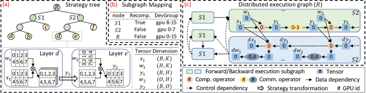
Figure 4: The strategy tree and corresponding distributed execution graph of DNN model in Figure 3.

IV-C Discussion and Comparison

Existing frameworks [19, 17, 35, 36] relies on computation graph to unify the parallelization space including computation, memory and schedule. However, Proteus focuses accurate performance modeling for a parallelization strategy, while these frameworks are designed for automated parallelization and they will search over all combinations of subgraphs. Explicitly modeling parallelization strategies is necessary for performance modeling, but it is quite hard to specify a complex parallelization strategy for a DNN model in prior automated parallelization works.

GSPMD [37] develops powerful programming APIs to specify parallelization strategies for different DNN layers, but the subgraph-level strategy is only supported for identical DNN blocks with tailored vectorized_map API. Furthermore, changing parallelization strategy also takes great efforts to rewrite the model. Our strategy tree unifies parallelization strategies at different levels and decouples parallelization strategy from model expression. By adjusting the strategy tree instead of the DNN model, Proteus can change the parallelization strategy for a DNN.

V Execution Graph Compiler

This section describes Proteus’s execution graph compiler, which connects high level parallelization strategies with low level execution. Given a strategy tree, the compiler creates a distributed execution graph by splitting tensors and computation operators and inserting communication operators and control dependencies.

V-A Graph Compilation

Figure 4 illustrates the workflow of execution graph compiler. Proteus first divides the DNN model into disjoint subgraphs based on its DevGroup, which defines a set of devices, in order to parallelize the computations of different micro-batches. The DevGroup of a tree node is composed of all of its children nodes’ DevGroups. Proteus splits all divisible nodes in breadth-first order from root node and a node cannot be divided unless all of its children nodes share some devices. Figure 4b shows the DevGroups of three nodes. The DevGroup of node $S2$ is "gpu 0-7" because layer $d$ and $e$ are partitioned and mapped to these devices. The root node $R$ is divided into 2 subgraphs since node $S1$ and $S2$ share no devices and they are not divisible.

Proteus then compiles each subgraph into a forward and backward execution subgraph as showed in Figure 4c. Tensors and operators are split into small partitions such that each partition resides on and is executed by one device. Communication operators, data and control dependencies are added to ensure the computational equivalence.

Data dependency. Each tensor and operator has a parallel configuration that defines the partition and mapping, as discussed in Section IV-B. Due to the data dependency between tensors and operators, Proteus can infer a parallel configuration for each input and output tensor of operators. Once the two parallel configurations of a tensor are inconsistent, Proteus automatically inserts communication operators via strategy transformation to adjust the parallel configuration, otherwise Proteus reuses original tensor partitions. Figure 4 shows the strategy transformation of tensor $y_{1}$. Layer $e$ partitions $y_{1}$ into 2 parts and each part replicates on 4 GPUs, but layer $d$ partitions $y_{1}$ into 8 partial tensors on 1 GPU. Proteus adds communication operators between $y_{1}$ in the execution subgraph of $S$2 to handle this inconsistency.

For a subgraph with recomputation enabled, Proteus compiles it into two forward and one backward execution subgraphs and adjust the data dependency accordingly. The backward subgraph depends on one forward subgraph (i.e. recomputation subgraph) and the other subgraph can be immediately released after execution (e.g. $S$1 in Figure 4c).

Control dependency. Control dependencies are inserted between execution subgraphs to follow the training schedule defined by the schedule config in non-leaf nodes. First, the forward subgraphs are control dependent on their corresponding backward subgraphs to limit peak memory consumption. Second, Proteus also adds control dependency for recomputation subgraphs such that they are executed immediately before the backward subgraphs. In Figure 4c, node $S$1 has two forward subgraphs and one of them is control dependent on the backward of node $S$2.

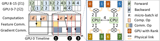
(a) Execution timeline.

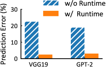
(b) Prediction error.

Figure 5: (a) The execution timeline and runtime behaviors of the distributed execution graph in Figure 4. The number on gray link denotes the number of groups that share the link. (b) Comparison of prediction errors for modeling runtime behaviors or not.

V-B Strategy Transformation

Strategy transformation converts tensors to desired parallel configurations with appropriate communication primitives. Proteus automatically infers collective communication primitives (e.g. All-Reduce [38]), failing over to point-to-point communication if necessary. Since different primitives features distinct communication patterns, Proteus uses pattern matching to infer collective communication operators and corresponding communication groups.

Proteus currently supports commonly used communication primitives in modern DL frameworks [21, 22]. Prior work proposes new communication primitives, such as hierarchical reduce [39, 40] and CollectivePermute [37], to accelerate the communication. Proteus can be extended by including more candidate patterns.

VI Hierarchical Topo-Aware Executor

This section describes Proteus’s Hierarchical Topo-Aware Executor (HTAE), which simulates the schedule and runtime behaviors of a distributed execution graph and predicts the training throughput.

VI-A Performance Characterization

Before introducing the design of HTAE, we first characterize the performance of distributed DNN training using the example of Figure 5(a), which illustrates the execution timeline and runtime behaviors of Figure 4. The forward and backward execution subgraphs are interleaved and the execution of $S1$ and $S2$ is parallelized on different GPU groups. Operators in Figure 4c consist of three types that can be executed simultaneously: computation, feature and gradient communication operators, and they are scheduled into three streams following data dependency. Modeling the training performance is to model the execution timeline, including schedule, computation and communication.

Runtime Behavior. Prior work [29, 28, 30, 17] assumes that the operator cost is fixed and focuses on modeling the performance of single operator. The training speed of a DNN is the summation of all the operators’ costs. However, runtime behavior, which is ignored in prior work, has emerged as a critical aspect determining training performance under today’s sophisticated parallelization strategies and optimizations. It is crucial to model runtime behaviors towards an accurate performance predictor since they can affect the execution cost of operators. Figure 5(b) shows that ignoring runtime behaviors results in large prediction error on a cluster with 32 GPUs.

We find that major runtime behaviors can be categorized into two types. First, bandwidth sharing describes the scenarios that different communication operators compete for bandwidth (Figure 5(a)❶,❸). Second, comp-comm overlap refers to the overlap of computation and communication operators (Figure 5(a)❷). In addition, different computation operators could be overlapped on single GPU [41], Proteus does not model such scenario since it is rarely used in distributed DNN training. Figure 5(a)❸ shows an example of bandwidth sharing by mapping gradient communication operators to a single node machine. The gradient communication includes 4 groups indicated by the GPU color: {{0, 4}, {1, 5}, {2, 6}, {3, 7}}, and their costs rise due to the competition for available bandwidth of scarce physical links.

Proteus is the first system to study and model runtime behaviors for distributed DNN training. Unlike prior analytical frameworks [29, 30], Proteus predicts training performance via simulation since runtime behaviors only occur during execution.

VI-B Simulator Design

Figure 6 shows the design of Proteus’s two level simulator, HTAE. The first level is scheduler, which consists of several second level executors. Different schedulers can time-share executors. To predict the performance, HTAE first gets single operator cost with op estimator (Section VII) and then simulates the schedule of subgraphs and operators to discover runtime behaviors. During simulation, operator cost are adapted to model runtime behaviors considering the cluster topology.

Cluster Configuration. Cluster Configuration describes the topology of training cluster. There are two types of configurable parameters in device topology. For intra-node topology, we can set device type, device memory, number of devices in a node and the intra-node connection, which describes the physical connections among devices (e.g. GPUs and CPUs). For inter-node topology, we can specify the number of nodes and inter-node connection bandwidth.

Scheduler. Each scheduler is assigned several forward and backward execution subgraphs, and it interleaves the execution of them based on data and control dependencies to balance micro-batch parallelism and peak memory consumption. The scheduler first selects current execution state (forward or backward), then it chooses one subgraph from available dependency-free execution subgraphs. It alternates different backward subgraphs and prefers forward subgraph that enables backward execution. After determining the subgraph to be executed, the scheduler dispatches initial tasks to executors and begin executing.

Executor. The executor schedules the execution of operators for a subgraph and records the peak memory consumption. Each executor contains a computation queue, a feature communication queue and a gradient communication queue (Figure 6). Operators in different queues can be executed concurrently such that achieving comp-comm overlap. By separating feature and gradient communication queue, Proteus makes it possible to overlap feature and gradient communication and avoid feature communication blocked by gradient communication.

The executor executes computation and communication alternatively. It pops a computation operator from the queue for computation execution and pops one feature and one gradient communication operator at the same time for communication execution. These operators are first sent to the runtime behavior detector to check runtime behaviors and executed afterwards. During execution, the operator cost will be accumulated to count the time cost for each queue separately. The execution of operators will decrease the number of dependencies of their consumers and dependency-free operators will be put into the corresponding queue.

Memory Consumption. Proteus predicts whether a parallelization strategy will out-of-memory (OOM) by monitoring the memory consumption of executors. During execution, each operator reads and writes some tensors. HTAE monitors executor memory footprint by recording these tensor activities. When writing a new tensor, HTAE tracks its memory consumption and reference counter. The memory will be released when the reference counter decreases to zero.

VI-C Modeling Runtime Behaviors

As previously discussed, the operator cost may change during execution due to complex runtime behaviors. The runtime behavior detector checks runtime behaviors for all operators and adapt operator cost accordingly. To enable efficient detection, it keeps execution history records of different execution streams.

Bandwidth Sharing. There are two types of bandwidth sharing. One is inside a group of gradient or feature communication operators (Figure 5(a)❸), and the other is between a group of gradient and feature communication operators (Figure 5(a)❶). These operators transfer datas within different device groups and compete for bandwidth of shared physical links. To model this behavior, Proteus assumes that concurrent operators fairly share the bandwidth of a physical link and detects how many communication groups share a link during execution. We find this assumption generally holds in practice.

Proteus first checks bandwidth sharing for feature and gradient communication operators separately by mapping communication groups to cluster topology. Figure 7 shows the hierarchy of physical links in a cluster and Proteus detects bandwidth sharing following this hierarchy. Proteus starts from NIC bandwidth sharing. Each communication group is split into sub-groups such that each sub-group is composed of devices in the same node. The groups that consist of more than two sub-groups fairly share the bandwidth of NIC. Proteus checks all the physical links from top to bottom.

Proteus finally detects the intersection effects of feature and gradient communication groups. Since the communication volumes and operations of these groups may different, Proteus only adapt operator cost for the overlapped parts. The detection algorithm is the same as the first step, except for that the communication groups include both feature and gradient communications.

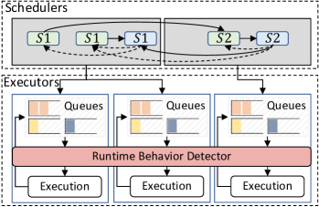
Figure 6: The design of hierarchical topo-aware executor.

Comp-Comm Overlap. In distributed DNN training, computation and gradient communication operators may overlap, because gradient communication operators can be launched asynchronously and feature communication operators usually block the computation stream. To detect comp-comm overlap, Proteus keeps the start and end time of operators. When executing a computation (communication) operator, Proteus considers it overlapped if it finds a gradient communication (computation) operator in execution.

Proteus introduces an overlap factor $\gamma$ to model the effect of comp-comm overlap. When finding an operator overlapped, its cost will increase by $\gamma$. This is motivated by the observation that operator costs increase by about the same percentage on average during overlap.

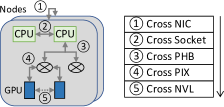
Figure 7: The hierarchy of bandwidth sharing.

To obtain $\gamma$, we profile the speeds of backward pass with and without overlapping in data parallel training and $\gamma$ is set to the increase ratio. As $\gamma$ is fixed for the type of machine and DNN model, we can get $\gamma$ in advance with few cost. Prior works [42, 43] also try to model the effect of comp-comm overlap. For example, Pollux [42] introduces a learnable parameter $\eta$ to model the data parallel training speed by combining computation time $T_{grad}$ and gradient communication time $T_{sync}$ with $({T_{grad}}^{\eta}+{T_{sync}}^{\eta})^{1/\eta}$. These works target on data parallel training, and we find our simple formulation works pretty well with complex parallelization strategies (discussed latter in Section VIII-D).

VII Implementation

Proteus is implemented as a standard python library ($\sim 9$K LoC). Proteus follows PyTorch [21] API to build model.

Construction of Strategy Tree. DNN models consists of modules that perform operations on data. A module is roughly equivalent to a DNN layer, and different modules can be nested together to construct a complex module. Proteus exploits the module structure to create a strategy tree from top to bottom in depth-first manner. Non-leaf nodes correspond to complex modules and leaf nodes correspond to layers. The root node represents the entire DNN model. Proteus tracks the construction of modules/layers and creates corresponding non-leaf/leaf nodes on the tree. The construction of strategy tree preserves the structure of DNN model and makes it easier to specify parallelization strategy for nodes.

Strategy Propagation. Proteus develops a strategy propagation algorithm to ease the programming difficulty of parallelization strategies. For a complete parallelization strategy, programmers are required to specify parallel configurations for critical leaf and non-leaf nodes. Proteus will propagate the parallel configurations to the other nodes.

Proteus first propagates parallel configurations from top to bottom following tree structure. The schedule config of a non-leaf node is inherited from its parent node unless explicitly defined. Proteus then propagates parallel configurations among leaf nodes following data dependency. The propagation proceeds in topological order and includes two steps: forward graph propagation and backward graph propagation. Proteus infers the memory config of a tensor according to its producer’s computation config and infers the computation config of an operator according to its inputs’ memory config.

TABLE II: Overview of the six benchmark models evaluated.

Task	Model	#Params	Dataset
Vision	ResNet50 [1]	25.6M	Synthetic
	Inception_V3[44]	23.8M
	VGG19 [45]	137M
NLP	GPT-2 [5]	117M
	GPT-1.5B [5]	1.5B
Recommendation	DLRM [46]	516M

Op Estimator. The op estimator predicts the operator cost for all operators in the distributed execution graph. It contains a profiler and analyzer. Since Proteus focuses on modeling runtime behaviors, the profiler obtains the time cost of computation operators by profiling them on target hardware, which costs little. There are lots of performance models to estimate single operator cost [23, 24, 25]. Proteus can be extended to adopt such models.

TABLE III: Overview of hardware configurations evaluated.

Config	#Node	#GPU per Node	Intra-node	Inter-node
HC1	1	8$\times$TitanXp	PCI-e	N/A
HC2	4	8$\times$V100	NVLink	100 Gbps
HC3	2	8$\times$A100	NVLink	200 Gbps

The analyzer estimates communication cost with $\alpha$-$\beta$ model [47]. It estimates the bandwidth of a communication group according to the detailed cluster topology. When estimating the time cost of a collective operation, a correction factor is applied to revise the bandwidth to reflect the characteristics of different collective operations. To simplify implementation, we utilize NCCL topo detection algorithm [38] to find all the communication channels of a communication group and its bandwidth is the summation of these channels.

VIII Evaluation

VIII-A Methodology

All the experiments are conducted with PyTorch 1.8 (CUDA 10.1, cuDNN 7.6.5 and NCCL 2.7.8).

Benchmarks. Table II summarizes the six representative DNN models that we used as benchmarks, they are widely used in prior works [30, 17, 25, 19]. We evaluate throughput with synthetic dataset, which ignores the data loading latency. Modeling real-world dataset is orthogonal to Proteus.

Hardware Configurations. Proteus is evaluated across three different hardware configurations. Table III summarizes the cluster type and size, intra- and inter-node connections.

VIII-B Simulation Accuracy

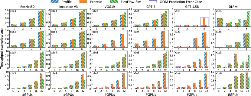
Figure 8: Throughput of DNN models on different hardware configurations with distinct parallelization strategies. The parallelization strategies from top to bottom row are $S1$ ($HC1$), $S2$ ($HC1$), $S1$ ($HC2$) and $S2$ ($HC2$), respectively. o: out of memory, $\times$: unsupported strategy.

To evaluate Proteus across a wide variety of parallelization strategies, we evaluate each model with 2 popular parallelization strategies. One is most commonly used parallelization strategy ($S1$), the other is the optimal expert-designed parallelization strategy ($S2$). Since Proteus is aimed at accurate performance modeling rather than discovering new parallelization strategies, and implementing entirely new parallelization strategies is difficult, we do not evaluate Proteus on less commonly used parallelization strategies. But the parallelization strategies we tested already cover both operator- and subgraph-level strategies.

Since the most commonly used parallelization strategy is data parallelism, Proteus uses data parallelism or its variants as $S1$ for six DNNs. To enable data parallelism training of large model, Proteus combines memory optimization (ZeRO [14]) and recomputation in $S1$ to evaluate GPT-1.5B. Expert-designed parallelization strategies ($S2$) exhibits more diverse patterns. ResNet50 and Inception_V3 partitions data and output channels, while VGG19 and GPT-2 partitions data, output channels and reduction dimensions for computation parallelization. The $S2$ of GPT-1.5B combines op shard, pipeline and recomputation. DLRM partitions huge embedding table in $S2$ to optimize memory footprint.

Figure 8 shows the simulation results of various DNN models on two hardware configurations ($HC1$ and $HC2$) and Table IV displays the overall results on three hardware configurations. Proteus delivers an accurate performance model and achieves $3.0\%$ average prediction error for training throughput. Out of 180 simulation results, Proteus’s estimation of OOM is incorrect only under 2 cases (blue box in Figure 8).

Proteus is the first standalone simulator that targets on simulating complex parallelization strategies. The most related and representative cost-model and simulator is Paleo [30] and FlexFlow [17], respectively. Paleo [30] is an analytical cost-model. It delivers high prediction error on single GPU (ResNet50 ($59.8\%$), Inception_V3 ($40\%$)) and does not support GPT, DLRM models and complex parallelization strategies. Therefore, we did not dive into Paleo and show the results. FlexFlow [17] is an automated parallelization framework on SOAP space. To compare generated parallelization strategies, it internally tailors a simulator to simulate the training throughput.

To compare Proteus and FlexFlow, we re-implement its simulator as FlexFlow-Sim. To support realistic simulation, FlexFlow-Sim inserts collective communication operators for strategy transformation instead of point-to-point operators as described in FlexFlow paper. The comparison results are shown in Figure 8 and Table IV. The average prediction error for FlexFlow is $12.4\%$, which is $9.4\%$ higher than Proteus. Among all the test cases, the maximum error is $14.7\%$ and $137.9\%$ for Proteus and FlexFlow, respectively. For the total 180 training tasks, FlexFlow fails to estimate the performance of 1/3 of them. Figure 8 also shows that the prediction error of FlexFlow-Sim becomes larger as the number of GPUs increases.

We find that Proteus outperforms FlexFlow mainly in three aspects. 1) Proteus can be applied to a much larger parallelization strategy space with the abstraction of strategy tree. 2) FlexFlow ignores complex runtime behaviors thus cannot accurately model the training throughput. 3) FlexFlow’s communication bandwidth estimation ignores fine-grained cluster topology. For example, FlexFlow delivers high prediction error for DLRM model, where communication dominates.

TABLE IV: Comparison of average and maximum prediction error of Proteus and FlexFlow-Sim (FF-Sim). Each strategy contains 15 results on 3 hardware configurations.

Model	Strategy	Avg Error (%)		Max Error (%)
		Proteus	FF-Sim	Proteus	FF-Sim
ResNet50	S1	2.09	3.59	6.00	8.69
	S2	2.30	5.98	5.77	35.65
Inception_V3	S1	3.24	5.53	7.52	11.71
	S2	3.19	6.57	7.97	36.73
VGG19	S1	1.97	8.11	4.97	28.17
	S2	1.68	✗	6.64	✗
GPT-2	S1	2.56	6.97	6.20	24.14
	S2	2.31	✗	11.38	✗
GPT-1.5B	S1	3.91	✗	8.09	✗
	S2	3.65	✗	9.92	✗
DLRM	S1	5.07	48.14	14.68	137.89
	S2	4.55	14.05	11.44	114.63

VIII-C Parallelization Strategy Comparison

Comparing the training throughput of various parallelization strategies is an important problem in designing and understanding high performance parallelization strategies. In this section, we use GPT-2 as benchmark because GPT model is the most popular and widely used model to study all kinds of parallelization strategies and these strategies can generalize to other models. In these experiments, we select 4 parallelizable dimensions across operator- and subgraph level strategies and represent the parallelization strategy as $DP\times MP\times PP(n\_micro\_batch)$ and $DP$, $MP$ and $PP$ is the degree of data, model and pipeline parallelism. The global batch size is 8 and 64 for HC1 and HC2 respectively.

TABLE V: The prediction error and rank of throughput for GPT-2 with different parallelization strategies on HC1 and HC2. Rank is denoted in the format of truth / predicted rank.

HC1			HC2
Strategy	Error	Rank	Strategy	Error	Rank
8$\times$1$\times$1 ($1$)	$2.34\%$	2 / 2	16$\times$1$\times$1 ($1$)	$3.38\%$	1 / 1
4$\times$2$\times$1 ($1$)	$2.92\%$	1 / 1	8$\times$2$\times$1 ($1$)	$2.89\%$	2 / 2
2$\times$4$\times$1 ($1$)	$2.43\%$	3 / 3	4$\times$4$\times$1 ($1$)	$5.87\%$	3 / 3
1$\times$8$\times$1 ($1$)	$1.77\%$	5 / 5	2$\times$8$\times$1 ($1$)	$3.88\%$	4 / 4
2$\times$2$\times$2 ($1$)	$2.54\%$	6 / 6	8$\times$1$\times$2 ($4$)	$3.60\%$	6 / 6
2$\times$2$\times$2 ($2$)	$1.60\%$	4 / 4	8$\times$1$\times$2 ($8$)	$2.99\%$	5 / 5
			2$\times$4$\times$2 ($4$)	$5.64\%$	7 / 7

Table V shows the simulation results of GPT-2 with various parallelization strategies. For these parallelization strategies, Proteus can accurately model the performance and achieves $3.2\%$ average prediction error. Order preservation is an important feature in strategy comparison and Proteus maintains the rank of diverse parallelization strategies. Table V demonstrates that HC2 prefers data parallelism training, since hybrid model parallelism shares the bandwidth of IB net, and pipeline parallelism introduces bubbles during training, which will decrease the training throughput. The simulation results also confirms that pipeline efficiency can be improved by injecting more micro batches. HC1 consists of a single NUMA node, and the 2-way model parallelism can fully utilize the QPI links between two CPU sockets, thus achieving highest throughput.

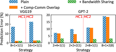
Figure 9: The prediction error of VGG19 and GPT-2 with different components. Plain: Proteus without runtime behavior detector.

VIII-D Runtime Behavior Ablation Study

To study the effective of runtime behavior detector, we test the throughput of VGG19 and GPT-2 on HC1 and HC2 with different parallelization strategies. For VGG19, we use batch size 32 per GPU with data parallelism training. For GPT-2, the global batch size is 8 and 64 on HC1 and HC2 with hybrid op shard and pipeline parallelism. Figure 9 shows that runtime behavior detector can greatly improve the simulation accuracy of throughput (average error: Plain ($14.4\%$) vs Proteus ($2.4\%$)). VGG19 is very sensitive to comm-comp overlap, hence introducing overlap factor can significantly improve the prediction accuracy. As there is no bandwidth sharing in data parallelism training, prediction error of VGG19 keeps after adding bandwidth sharing. In contrast, GPT-2 is more sensitive to bandwidth sharing which is especially common in complex parallelization strategies. Therefore, the throughput prediction error reduces remarkably after modeling bandwidth sharing.

VIII-E Simulation Cost

To evaluate the simulation cost of Proteus, we measure the time it takes to evaluate VGG19 and GPT-2 on HC2 with data parallelism. Since the cost of computation operators can be profiled in advance, we only evaluate the time cost of execution graph compiler and HTAE. Table VI demonstrates that Proteus takes seconds to simulate the performance of DNNs with a large number of GPUs. We believe this cost is acceptable to evaluate a specified parallelization strategy since Proteus provides a fine-grained simulation without requiring GPU resources. In contrast, profiling a general parallelization strategy will take a lot of effort and GPU resources.

TABLE VI: Simulation cost of Proteus on HC2 in seconds.

#GPUs	VGG19			GPT-2
	compile	exe.	total	compile	exe.	total
1	0.033	0.006	0.039	0.188	0.070	0.258
2	0.053	0.407	0.460	0.341	0.450	0.792
4	0.114	0.530	0.644	0.504	0.692	1.196
8	0.170	0.563	0.733	1.008	0.873	1.881
16	0.336	0.630	0.966	1.966	1.172	3.138
32	0.777	0.921	1.698	4.143	2.123	6.265

IX Related Work

Handcrafted Parallelization Strategies are designed to optimize distributed DNN training. One wired trick [48] introduces model parallelism for linear layers to accelerate AlexNet. Megatron-LM [10] presents an expert-designed strategy to expedite transformer models combining data, model and pipeline parallelism. DeepSpeed [33] introduces ZeRO to reduce memory footprint by partitioning model states across data parallel processes. Recomputation [32] utilizes tensor rematerialization to decrease memory consumption. Proteus can model the performance of these manual designed strategies thus assisting their analysis and optimization.

Automatic Parallelization. FlexFlow [17] and Tofu [18] proposes SOAP and partition-n-reduce space to parallelize operators. GSPMD [37] introduces a more general parallelization space by partitioning all parallelizable dimensions of tensors. DAPPLE [19] and PipeDream [20] optimize parallelization strategies in data and pipeline parallelization space. Alpa [35] combines data, model and pipeline parallelism and proposes a inter-operator and intra-operator parallelization space. Existing automatic approaches focus on exploring the space of computation parallelization, while our work introduces a unified parallelization strategy space considering computation parallelization and memory optimization at operator level and schedule at subgraph level.

Performance Model. Previous works propose analytical performance models for DNN training on single GPU [25, 23, 24] or on multiple GPUs with data parallelism or hybrid data and model parallelism [29, 30, 28]. These approaches are not applicable to increasingly complex training workload and strategies. FlexFlow [17] introduces a simulation model to estimate the cost of a SOAP strategy, but it is not designed to capture the cost of general strategies and runtime behaviors. Proteus aims to provide a general simulation performance model for various parallelization strategies.

X Conclusion

In this work, we present Proteus to simulate the performance of distributed DNN training strategies on diverse clusters. Proteus features strategy tree to model unified parallelization strategy space and hierarchical topo-aware executor to model runtime behaviors of computation and communication operators accurately. We can leverage Proteus to analyze and optimize the performance of general parallelization strategies.

References

- [1] K. He, X. Zhang, S. Ren, and J. Sun, “Deep residual learning for image recognition,” in Proceedings of the IEEE conference on computer vision and pattern recognition, 2016, pp. 770–778.
- [2] A. Krizhevsky, I. Sutskever, and G. E. Hinton, “Imagenet classification with deep convolutional neural networks,” Advances in neural information processing systems, vol. 25, pp. 1097–1105, 2012.
- [3] A. Vaswani, N. Shazeer, N. Parmar, J. Uszkoreit, L. Jones, A. N. Gomez, Ł. Kaiser, and I. Polosukhin, “Attention is all you need,” in Advances in neural information processing systems, 2017, pp. 5998–6008.
- [4] A. Radford, K. Narasimhan, T. Salimans, and I. Sutskever, “Improving language understanding by generative pre-training,” 2018.
- [5] A. Radford, J. Wu, R. Child, D. Luan, D. Amodei, and I. Sutskever, “Language models are unsupervised multitask learners,” OpenAI blog, vol. 1, no. 8, p. 9, 2019.
- [6] T. B. Brown, B. Mann, N. Ryder, M. Subbiah, J. Kaplan, P. Dhariwal, A. Neelakantan, P. Shyam, G. Sastry, A. Askell, S. Agarwal, A. Herbert-Voss, G. Krueger, T. Henighan, R. Child, A. Ramesh, D. M. Ziegler, J. Wu, C. Winter, C. Hesse, M. Chen, E. Sigler, M. Litwin, S. Gray, B. Chess, J. Clark, C. Berner, S. McCandlish, A. Radford, I. Sutskever, and D. Amodei, “Language models are few-shot learners,” in Advances in Neural Information Processing Systems 33: Annual Conference on Neural Information Processing Systems 2020, NeurIPS 2020, December 6-12, 2020, virtual, H. Larochelle, M. Ranzato, R. Hadsell, M. Balcan, and H. Lin, Eds., 2020.
- [7] D. Lepikhin, H. Lee, Y. Xu, D. Chen, O. Firat, Y. Huang, M. Krikun, N. Shazeer, and Z. Chen, “Gshard: Scaling giant models with conditional computation and automatic sharding,” in 9th International Conference on Learning Representations, ICLR 2021, Virtual Event, Austria, May 3-7, 2021. OpenReview.net, 2021.
- [8] J. Dean, G. Corrado, R. Monga, K. Chen, M. Devin, Q. V. Le, M. Z. Mao, M. Ranzato, A. W. Senior, P. A. Tucker, K. Yang, and A. Y. Ng, “Large scale distributed deep networks,” in Advances in Neural Information Processing Systems 25: 26th Annual Conference on Neural Information Processing Systems 2012. Proceedings of a meeting held December 3-6, 2012, Lake Tahoe, Nevada, United States, P. L. Bartlett, F. C. N. Pereira, C. J. C. Burges, L. Bottou, and K. Q. Weinberger, Eds., 2012, pp. 1232–1240.
- [9] P. Mattson, C. Cheng, G. F. Diamos, C. Coleman, P. Micikevicius, D. A. Patterson, H. Tang, G. Wei, P. Bailis, V. Bittorf, D. Brooks, D. Chen, D. Dutta, U. Gupta, K. M. Hazelwood, A. Hock, X. Huang, D. Kang, D. Kanter, N. Kumar, J. Liao, D. Narayanan, T. Oguntebi, G. Pekhimenko, L. Pentecost, V. J. Reddi, T. Robie, T. S. John, C. Wu, L. Xu, C. Young, and M. Zaharia, “Mlperf training benchmark,” in Proceedings of Machine Learning and Systems 2020, MLSys 2020, Austin, TX, USA, March 2-4, 2020, I. S. Dhillon, D. S. Papailiopoulos, and V. Sze, Eds. mlsys.org, 2020.
- [10] M. Shoeybi, M. Patwary, R. Puri, P. LeGresley, J. Casper, and B. Catanzaro, “Megatron-lm: Training multi-billion parameter language models using model parallelism,” arXiv preprint arXiv:1909.08053, 2019.
- [11] D. Narayanan, M. Shoeybi, J. Casper, P. LeGresley, M. Patwary, V. Korthikanti, D. Vainbrand, P. Kashinkunti, J. Bernauer, B. Catanzaro, A. Phanishayee, and M. Zaharia, “Efficient large-scale language model training on GPU clusters using megatron-lm,” in SC ’21: The International Conference for High Performance Computing, Networking, Storage and Analysis, St. Louis, Missouri, USA, November 14 - 19, 2021. ACM, 2021, pp. 58:1–58:15.
- [12] Z. Li, S. Zhuang, S. Guo, D. Zhuo, H. Zhang, D. Song, and I. Stoica, “Terapipe: Token-level pipeline parallelism for training large-scale language models,” arXiv preprint arXiv:2102.07988, 2021.
- [13] S. Rajbhandari, J. Rasley, O. Ruwase, and Y. He, “Zero: Memory optimizations toward training trillion parameter models,” in SC20: International Conference for High Performance Computing, Networking, Storage and Analysis. IEEE, 2020, pp. 1–16.
- [14] J. Ren, S. Rajbhandari, R. Y. Aminabadi, O. Ruwase, S. Yang, M. Zhang, D. Li, and Y. He, “Zero-offload: Democratizing billion-scale model training,” arXiv preprint arXiv:2101.06840, 2021.
- [15] S. Rajbhandari, O. Ruwase, J. Rasley, S. Smith, and Y. He, “Zero-infinity: Breaking the gpu memory wall for extreme scale deep learning,” arXiv preprint arXiv:2104.07857, 2021.
- [16] J. Fang, Y. Yu, S. Li, Y. You, and J. Zhou, “Patrickstar: Parallel training of pre-trained models via a chunk-based memory management,” CoRR, vol. abs/2108.05818, 2021.
- [17] Z. Jia, M. Zaharia, and A. Aiken, “Beyond data and model parallelism for deep neural networks.” Proceedings of Machine Learning and Systems, vol. 1, pp. 1–13, 2019.
- [18] M. Wang, C.-c. Huang, and J. Li, “Supporting very large models using automatic dataflow graph partitioning,” in Proceedings of the Fourteenth EuroSys Conference 2019, 2019, pp. 1–17.
- [19] S. Fan, Y. Rong, C. Meng, Z. Cao, S. Wang, Z. Zheng, C. Wu, G. Long, J. Yang, L. Xia, L. Diao, X. Liu, and W. Lin, “DAPPLE: a pipelined data parallel approach for training large models,” in PPoPP ’21: 26th ACM SIGPLAN Symposium on Principles and Practice of Parallel Programming, Virtual Event, Republic of Korea, February 27- March 3, 2021. ACM, 2021, pp. 431–445.
- [20] D. Narayanan, A. Harlap, A. Phanishayee, V. Seshadri, N. R. Devanur, G. R. Ganger, P. B. Gibbons, and M. Zaharia, “Pipedream: generalized pipeline parallelism for dnn training,” in Proceedings of the 27th ACM Symposium on Operating Systems Principles, 2019, pp. 1–15.
- [21] A. Paszke, S. Gross, F. Massa, A. Lerer, J. Bradbury, G. Chanan, T. Killeen, Z. Lin, N. Gimelshein, L. Antiga, A. Desmaison, A. Köpf, E. Z. Yang, Z. DeVito, M. Raison, A. Tejani, S. Chilamkurthy, B. Steiner, L. Fang, J. Bai, and S. Chintala, “Pytorch: An imperative style, high-performance deep learning library,” in Advances in Neural Information Processing Systems 32: Annual Conference on Neural Information Processing Systems 2019, NeurIPS 2019, December 8-14, 2019, Vancouver, BC, Canada, 2019, pp. 8024–8035.
- [22] M. Abadi, P. Barham, J. Chen, Z. Chen, A. Davis, J. Dean, M. Devin, S. Ghemawat, G. Irving, M. Isard, M. Kudlur, J. Levenberg, R. Monga, S. Moore, D. G. Murray, B. Steiner, P. A. Tucker, V. Vasudevan, P. Warden, M. Wicke, Y. Yu, and X. Zheng, “Tensorflow: A system for large-scale machine learning,” in 12th USENIX Symposium on Operating Systems Design and Implementation, OSDI 2016, Savannah, GA, USA, November 2-4, 2016. USENIX Association, 2016, pp. 265–283.
- [23] K. Kothapalli, R. Mukherjee, M. S. Rehman, S. Patidar, P. Narayanan, and K. Srinathan, “A performance prediction model for the cuda gpgpu platform,” in 2009 International Conference on High Performance Computing (HiPC). IEEE, 2009, pp. 463–472.
- [24] Y. Zhang and J. D. Owens, “A quantitative performance analysis model for gpu architectures,” in 2011 IEEE 17th international symposium on high performance computer architecture. IEEE, 2011, pp. 382–393.
- [25] G. Liu, S. Wang, and Y. Bao, “Seer: A time prediction model for cnns from gpu kernel’s view,” in 2021 30th International Conference on Parallel Architectures and Compilation Techniques (PACT). IEEE, 2021, pp. 173–185.
- [26] T. Chen, T. Moreau, Z. Jiang, L. Zheng, E. Q. Yan, H. Shen, M. Cowan, L. Wang, Y. Hu, L. Ceze, C. Guestrin, and A. Krishnamurthy, “TVM: an automated end-to-end optimizing compiler for deep learning,” in 13th USENIX Symposium on Operating Systems Design and Implementation, OSDI 2018, Carlsbad, CA, USA, October 8-10, 2018. USENIX Association, 2018, pp. 578–594.
- [27] R. Baghdadi, M. Merouani, M. Leghettas, K. Abdous, T. Arbaoui, K. Benatchba, and S. P. Amarasinghe, “A deep learning based cost model for automatic code optimization,” in Proceedings of Machine Learning and Systems, MLSys 2021, virtual, April 5-9, 2021. mlsys.org, 2021.
- [28] Z. Pei, C. Li, X. Qin, X. Chen, and G. Wei, “Iteration time prediction for cnn in multi-gpu platform: modeling and analysis,” IEEE Access, vol. 7, pp. 64 788–64 797, 2019.
- [29] F. Yan, O. Ruwase, Y. He, and T. Chilimbi, “Performance modeling and scalability optimization of distributed deep learning systems,” in Proceedings of the 21th ACM SIGKDD International Conference on Knowledge Discovery and Data Mining, 2015, pp. 1355–1364.
- [30] H. Qi, E. R. Sparks, and A. Talwalkar, “Paleo: A performance model for deep neural networks,” in 5th International Conference on Learning Representations, ICLR 2017, Toulon, France, April 24-26, 2017, Conference Track Proceedings. OpenReview.net, 2017.
- [31] V. Elango, “Pase: Parallelization strategies for efficient dnn training,” in 2021 IEEE International Parallel and Distributed Processing Symposium (IPDPS). IEEE, 2021, pp. 1025–1034.
- [32] T. Chen, B. Xu, C. Zhang, and C. Guestrin, “Training deep nets with sublinear memory cost,” CoRR, vol. abs/1604.06174, 2016.
- [33] J. Rasley, S. Rajbhandari, O. Ruwase, and Y. He, “Deepspeed: System optimizations enable training deep learning models with over 100 billion parameters,” in Proceedings of the 26th ACM SIGKDD International Conference on Knowledge Discovery & Data Mining, 2020, pp. 3505–3506.
- [34] Y. Huang, Y. Cheng, A. Bapna, O. Firat, D. Chen, M. X. Chen, H. Lee, J. Ngiam, Q. V. Le, Y. Wu, and Z. Chen, “Gpipe: Efficient training of giant neural networks using pipeline parallelism,” in Advances in Neural Information Processing Systems 32: Annual Conference on Neural Information Processing Systems 2019, NeurIPS 2019, December 8-14, 2019, Vancouver, BC, Canada, 2019, pp. 103–112.
- [35] L. Zheng, Z. Li, H. Zhang, Y. Zhuang, Z. Chen, Y. Huang, Y. Wang, Y. Xu, D. Zhuo, E. P. Xing, J. E. Gonzalez, and I. Stoica, “Alpa: Automating inter- and intra-operator parallelism for distributed deep learning,” in 16th USENIX Symposium on Operating Systems Design and Implementation, OSDI 2022, Carlsbad, CA, USA, July 11-13, 2022, M. K. Aguilera and H. Weatherspoon, Eds. USENIX Association, 2022, pp. 559–578.
- [36] C. Unger, Z. Jia, W. Wu, S. Lin, M. Baines, C. E. Q. Narvaez, V. Ramakrishnaiah, N. Prajapati, P. S. McCormick, J. Mohd-Yusof, X. Luo, D. Mudigere, J. Park, M. Smelyanskiy, and A. Aiken, “Unity: Accelerating DNN training through joint optimization of algebraic transformations and parallelization,” in 16th USENIX Symposium on Operating Systems Design and Implementation, OSDI 2022, Carlsbad, CA, USA, July 11-13, 2022, M. K. Aguilera and H. Weatherspoon, Eds. USENIX Association, 2022, pp. 267–284.
- [37] Y. Xu, H. Lee, D. Chen, B. A. Hechtman, Y. Huang, R. Joshi, M. Krikun, D. Lepikhin, A. Ly, M. Maggioni, R. Pang, N. Shazeer, S. Wang, T. Wang, Y. Wu, and Z. Chen, “GSPMD: general and scalable parallelization for ML computation graphs,” CoRR, vol. abs/2105.04663, 2021.
- [38] “Nvidia nccl,” https://developer.nvidia.com/nccl, 2021.
- [39] H. Mikami, H. Suganuma, Y. Tanaka, Y. Kageyama et al., “Massively distributed sgd: Imagenet/resnet-50 training in a flash,” arXiv preprint arXiv:1811.05233, 2018.
- [40] Y. Ueno and R. Yokota, “Exhaustive study of hierarchical allreduce patterns for large messages between gpus,” in 19th IEEE/ACM International Symposium on Cluster, Cloud and Grid Computing, CCGRID 2019, Larnaca, Cyprus, May 14-17, 2019. IEEE, 2019, pp. 430–439.
- [41] Y. Ding, L. Zhu, Z. Jia, G. Pekhimenko, and S. Han, “IOS: inter-operator scheduler for CNN acceleration,” in Proceedings of Machine Learning and Systems 2021, MLSys 2021, virtual, April 5-9, 2021, A. Smola, A. Dimakis, and I. Stoica, Eds. mlsys.org, 2021.
- [42] A. Qiao, S. K. Choe, S. J. Subramanya, W. Neiswanger, Q. Ho, H. Zhang, G. R. Ganger, and E. P. Xing, “Pollux: Co-adaptive cluster scheduling for goodput-optimized deep learning,” in 15th USENIX Symposium on Operating Systems Design and Implementation (OSDI 21), 2021.
- [43] C. Yang, Z. Li, C. Ruan, G. Xu, C. Li, R. Chen, and F. Yan, “Perfestimator: A generic and extensible performance estimator for data parallel dnn training,” in 2021 IEEE/ACM International Workshop on Cloud Intelligence (CloudIntelligence), 2021, pp. 13–18.
- [44] C. Szegedy, V. Vanhoucke, S. Ioffe, J. Shlens, and Z. Wojna, “Rethinking the inception architecture for computer vision,” in Proceedings of the IEEE conference on computer vision and pattern recognition, 2016, pp. 2818–2826.
- [45] K. Simonyan and A. Zisserman, “Very deep convolutional networks for large-scale image recognition,” arXiv preprint arXiv:1409.1556, 2014.
- [46] M. Naumov, D. Mudigere, H. M. Shi, J. Huang, N. Sundaraman, J. Park, X. Wang, U. Gupta, C. Wu, A. G. Azzolini, D. Dzhulgakov, A. Mallevich, I. Cherniavskii, Y. Lu, R. Krishnamoorthi, A. Yu, V. Kondratenko, S. Pereira, X. Chen, W. Chen, V. Rao, B. Jia, L. Xiong, and M. Smelyanskiy, “Deep learning recommendation model for personalization and recommendation systems,” CoRR, vol. abs/1906.00091, 2019.
- [47] L. G. Valiant, “A bridging model for parallel computation,” Commun. ACM, vol. 33, no. 8, pp. 103–111, 1990.
- [48] A. Krizhevsky, “One weird trick for parallelizing convolutional neural networks,” arXiv preprint arXiv:1404.5997, 2014.