Less is More: Revisiting the Gaussian Mechanism for Differential Privacy

Abstract

Differential privacy (DP) via output perturbation has been a de facto standard for releasing query or computation results on sensitive data. Different variants of the classic Gaussian mechanism have been developed to reduce the magnitude of the noise and improve the utility of sanitized query results. However, we identify that all existing Gaussian mechanisms suffer from the curse of full-rank covariance matrices, and hence the expected accuracy losses of these mechanisms equal the trace of the covariance matrix of the noise. Particularly, for query results in $\mathbb{R}^{M}$ (or $\mathbb{R}^{M\times N}$ in a matrix form), in order to achieve $(\epsilon,\delta)$-DP, the expected accuracy loss of the classic Gaussian mechanism, that of the analytic Gaussian mechanism, and that of the Matrix-Variate Gaussian (MVG) mechanism are lower bounded by $C_{C}(\Delta f)^{2}$, $C_{A}(\Delta f)^{2}$, and $C_{M}(\Delta f)^{2}$, respectively, where $C_{C}=\frac{2\ln\left(\frac{1.25}{\delta}\right)}{\epsilon^{2}}M$, $C_{A}=\frac{\left(\Phi^{-1}(\delta)\right)^{2}+\epsilon}{\epsilon^{2}}M$, $C_{M}=\frac{\frac{5}{4}H_{r}+\frac{1}{4}H_{r,\frac{1}{2}}}{2\epsilon}MN$, $\Delta_{2}f$ is the $l_{2}$ sensitivity of the query function $f$, $\Phi(\cdot)^{-1}$ is the quantile function of the standard normal distribution, $H_{r}$ is the $r$th harmonic number, and $H_{r,\frac{1}{2}}$ is the $r$th harmonic number of order $\frac{1}{2}$.

To lift this curse, we design a Rank-1 Singular Multivariate Gaussian (R1SMG) mechanism. It achieves $(\epsilon,\delta)$-DP on query results in $\mathbb{R}^{M}$ by perturbing the results with noise following a singular multivariate Gaussian distribution, whose covariance matrix is a randomly generated rank-1 positive semi-definite matrix. In contrast, the classic Gaussian mechanism and its variants all consider deterministic full-rank covariance matrices. Our idea is motivated by a clue from Dwork et al.’s seminal work on the classic Gaussian mechanism that has been ignored in the literature: when projecting multivariate Gaussian noise with a full-rank covariance matrix onto a set of orthonormal basis in $\mathbb{R}^{M}$, only the coefficient of a single basis can contribute to the privacy guarantee.

This paper makes the following technical contributions.

(i) The R1SMG mechanisms achieves $(\epsilon,\delta)$-DP guarantee on query results in $\mathbb{R}^{M}$, while its expected accuracy loss is lower bounded by $C_{R}(\Delta_{2}f)^{2}$, where $C_{R}=\frac{2}{\epsilon\psi}$ and $\psi=\Big{(}\frac{\delta\Gamma(\frac{M-1}{2})}{\sqrt{\pi}\Gamma(\frac{M}{2})}\Big{)}^{\frac{2}{M-2}}$. We show that $C_{R}$ has a decreasing trend as $M$ increases, and converges to $\frac{2}{\epsilon}$ as $M$ approaches infinity. Therefore, the expected accuracy loss of the R1SMG mechanism is on a much lower order compared with that of the classic Gaussian mechanism, of the analytic Gaussian mechanism, and of the MVG mechanism.

(ii) Compared with other mechanisms, the R1SMG mechanism is more stable and less likely to generate noise with large magnitude that overwhelms the query results, because the kurtosis and skewness of the nondeterministic accuracy loss introduced by this mechanism is larger than that introduced by other mechanisms.

1 Introduction

Differential privacy (DP) [15, 17] has been increasingly recognized as the fundamental building block for privacy-preserving database query, sharing, and analysis. In this area, one important privacy guarantee is $(\epsilon,\delta)$-DP. It means that, except with a small probability of $\delta$, the presence or absence of any data record in a dataset cannot change the probability of observing a specific query result of the dataset by more than a multiplicative factor of $e^{\epsilon}$.

The classic Gaussian mechanism, proposed by Dwork et al. [15], is an essential tool to achieve $(\epsilon,\delta)$-DP. Particularly, when the output of a query function is a high dimensional vector, the classic Gaussian mechanism will add independent and identically distributed (i.i.d.) noise to each component of the result (see Definition 3 and [17, p. 261], [15, p. 3]).

This standard practice has spread widely into many fields. For example, a differentially private mechanism returns noisy answers to a set of queries by adding i.i.d. noise to each query result [35]. Privacy-preserving learning employs differentially private stochastic gradient descent through perturbing each component of the gradient with i.i.d. Gaussian noise [3]. Unfortunately, as we will show later, the adoption of the classic Gaussian mechanism greatly hinders the utility (accuracy) of the sanitized query results because the expected accuracy loss (Definition 1) of the classic Gaussian mechanism is on the order of $M(\Delta_{2}f)^{2}$, where $\Delta_{2}f$ is the $l_{2}$ sensitivity of the query function and $M$ is the dimension of the query results. We refer to this as the curse of full-rank covariance matrices.

Definition 1.

Accuracy Loss [35, 22]. The accuracy loss of a differentially private output perturbation mechanism ($\mathcal{M}$) is

$$\mathcal{L}=||\mathcal{M}(f(\bm{x}))-f(\bm{x})||_{2}^{2}=||\mathbf{n}||_{2}^{2},$$ (1)

where $\bm{x}$ denotes a dataset, $f(\bm{x})$ is the query result on dataset $\bm{x}$, and $\mathbf{n}$ is the noise vector added to the query result.

We can see from (1) that the accuracy loss is equal to the magnitude of the additive noise. Due to the randomness involved in the noise, $\mathcal{L}$ is nondeterministic. Thus, we investigate the expected value of accuracy loss, i.e., $\mathbb{E}[\mathcal{L}]$.

1.1 The Curse of Full-Rank Covariance Matrices

Here, we provide a high-level description on the identified curse of full-rank covariance matrices, while the details are deferred to Section  3.

Proposition 1.

The Identified Curse. Let $\bm{x}$ be a dataset, $f(\bm{x})\in\mathbb{R}^{M}$ the queried results, and $\mathbf{n}\in\mathbb{R}^{M}$ the perturbation noises introduced by the classic Gaussian mechanism (or its variants, e.g., the analytic Gaussian mechanism [5], and the Matrix-Variate Gaussian (MVG) mechanism [11]), respectively. Then, the expected accuracy loss is equal to the trace of the covariance matrix of the Gaussian noise $\mathbf{n}$, i.e., $\mathbb{E}[\mathcal{L}]=Tr[Cov(\mathbf{n})]$, where $Cov(\mathbf{n})$ denotes the covariance matrix of the noise $\mathbf{n}$.

Since existing Gaussian mechanisms always introduce noise that has a full-rank covariance matrix, i.e., $rank(Cov(\mathbf{n}))=M$, where $Cov(\mathbf{n})$ is symmetric and positive definite [10], $\mathbb{E}[\mathcal{L}]$ is equivalent to the summation of $M$ positive eigenvalues of $Cov(\mathbf{n})$ and hence generally high. In Section  3, we will prove Proposition 1 when $f(\bm{x})$ is in a vector form and in a matrix form under different variants of the classic Gaussian mechanism.

1.2 Lifting the Curse: Main Contributions

To lift the identified curse, we resort to the singular multivariate Gaussian distribution [28, 14, 40, 43, 30] (Definition 7) with a rank-1 covariance matrix and develop the Rank-1 Singular Multivariate Gaussian (R1SMG) mechanism. Our idea is motivated by an ignored clue in Dwork and Roth’s proof for the DP guarantee of the Gaussian mechanism [17]. Specifically, Dwork and Roth proved that by projecting the additive noise $\mathbf{n}\in\mathbb{R}^{M}$ onto a fixed set of orthonormal basis vectors (e.g., $\bm{b}_{1},\bm{b}_{2},\cdots,\bm{b}_{M}$), only the coefficient of a single basis vector (e.g., $\mathbf{n}^{T}\bm{b}_{1}$) contributes to the privacy guarantee (more details are deferred to Section 4). However, this important clue has been ignored in the literature. To the best of our knowledge, our work is the first to discover and leverage this ignored clue.

The main contributions of this paper are summarized as follows.

(1) A new DP Mechanism and Privacy Guarantee (Definition 8 and Theorem 5). We develop the R1SMG mechanism that can achieve $(\epsilon,\delta)$-DP guarantee on high dimensional query results $f(\bm{x})\in\mathbb{R}^{M}$ ($M>2$). The covariance matrix, denoted as $\bm{\Pi}$, of the noise introduced by the R1SMG mechanism is a random rank-1 symmetric positive semi-definite matrix, whose eigenvector is randomly sampled from the unit sphere embedded in $\mathbb{R}^{M}$. Let $\sigma_{*}$ be the eigenvalue of the rank-1 covariance matrix $\bm{\Pi}$. We prove that a sufficient condition for the R1SMG mechanism to achieve $(\epsilon,\delta)$-DP is $\sigma_{*}\geq\frac{2(\Delta_{2}f)^{2}}{\epsilon\psi}$, where $\Delta_{2}f$ is the $l_{2}$ sensitivity of the query function $f$, $\psi=\Big{(}\frac{\delta\Gamma(\frac{M-1}{2})}{\sqrt{\pi}\Gamma(\frac{M}{2})}\Big{)}^{\frac{2}{M-2}}$, and $\Gamma(\cdot)$ is Gamma function.

(2) Expected accuracy loss on a much lower order than that of existing Gaussian mechanisms. We prove that the expected accuracy loss of $f(\bm{x})$ caused by the R1SMG mechanism (i.e., $||{R1SMG}(f(\bm{x}))-f(\bm{x})||_{2}^{2}$) is lower bounded by $C_{R}(\Delta_{2}f)^{2}$, where $C_{R}=\frac{2}{\epsilon\psi}$ has a decreasing trend as $M$ increases and converges to $\frac{2}{\epsilon}$ as $M$ approaches infinity (Theorem 7). In contrast, the classic Gaussian, analytic Gaussian, and MVG mechanisms result in expected accuracy loss that is lower bounded by $C_{C}(\Delta f)^{2}$, $C_{A}(\Delta f)^{2}$, and $C_{M}(\Delta f)^{2}$, respectively, where $C_{C}=\frac{2\ln\left(\frac{1.25}{\delta}\right)}{\epsilon^{2}}M$, $C_{A}=\frac{\left(\Phi^{-1}(\delta)\right)^{2}+\epsilon}{\epsilon^{2}}M$, and $C_{M}=\frac{\frac{5}{4}H_{r}+\frac{1}{4}H_{r,\frac{1}{2}}}{2\epsilon}MN$ (for query results in $\mathbb{R}^{M\times N}$, i.e., in a matrix form). Therefore, by using the R1SMG mechanism, less is more in the sense that (i) $C_{R}$ has a decreasing trend, and (ii) noise of a much lower order magnitude is needed compared with that of existing Gaussian mechanisms.

(3) Higher stability of the perturbed results (Theorem 8 and 9). We theoretically show that the accuracy of the perturbed $f(\bm{x})$ obtained by the R1SMG mechanism is more stable than the other mechanisms. By “stable”, we mean that it is less likely for the R1SMG mechanism to generate noise with large magnitude that overwhelms $f(\bm{x})$.

(4) Applications. We perform three case studies, including differentially private 2D histogram query, principal component analysis, and deep learning, to validate that the R1SMG mechanism can significantly boost the utility of various applications by introducing less noise.

Table 1 summarizes and compares our proposed R1SMG mechanism with the classic Gaussian mechanism and its variants from the perspective of expected accuracy loss parameterized by the noise parameters and utility stability.

Mechanisms ($\mathcal{M}$)	Expected accuracy loss $\mathbb{E}_{\mathcal{M}}[\mathcal{L}]$	Stability (Section 6)
The classic Gaussian mechanism [15] (noise decided by variance $\sigma^{2}$ and dimension $f(\bm{x})\in\mathbb{R}^{M}$)	$\mathbb{E}_{classic}[\mathcal{L}]=Tr[\sigma^{2}\mathbf{I}_{M\times M}]\geq C_{C}(\Delta f)^{2}$, where $C_{C}=\frac{2\ln\left(\frac{1.25}{\delta}\right)}{\epsilon^{2}}M=\Theta(M)$. (Section 3.1)	unstable, i.e., likely to generate noise with large magnitude
The analytic Gaussian mechanism [5] (noise decided by variance $\sigma_{A}^{2}$ and dimension $f(\bm{x})\in\mathbb{R}^{M}$)	$\mathbb{E}_{analytic}[\mathcal{L}]=Tr[\sigma_{A}^{2}\mathbf{I}_{M\times M}]\geq C_{A}(\Delta f)^{2}$, where $C_{A}=\frac{\left(\Phi^{-1}(\delta)\right)^{2}+\epsilon}{\epsilon^{2}}M=\Theta(M)$. (Section 3.1)	unstable
The MVG mechanism [11] (noise decided by covariance matrices $\bm{\Sigma}$, $\bm{\Psi}$, and dimension $f(\bm{x})\in\mathbb{R}^{M\times N}$)	$\mathbb{E}_{MVG}[\mathcal{L}]=Tr[\bm{\Sigma}\otimes\bm{\Psi}]\geq C_{M}(\Delta f)^{2}$, where $C_{M}=\frac{\frac{5}{4}H_{r}+\frac{1}{4}H_{r,\frac{1}{2}}}{2\epsilon}MN=\Theta(MN)$. (Section 3.2)	unstable
The R1SMG mechanism (noise decided by a random rank-1 singular covariance matrix with only one nonzero eigenvalue $\sigma_{*}$)	$\mathbb{E}_{R1SMG}[\mathcal{L}]=Tr[\bm{\Pi}]=\sigma_{*}\geq C_{R}(\Delta_{2}f)^{2}$, where $C_{R}=\frac{2}{\epsilon\psi}$, $\psi=\Big{(}\frac{\delta\Gamma(\frac{M-1}{2})}{\sqrt{\pi}\Gamma(\frac{M}{2})}\Big{)}^{\frac{2}{M-2}}$, and $C_{R}=\Theta(1)$. $C_{R}$ has a decreasing trend as M increases, and converges to $\frac{2}{\epsilon}$ as $M$ approaches infinity. (Section 5.3)	stable, i.e., unlikely to generate noise with large magnitude

Table 1: Comparisons between the R1SMG mechanism and the classic Gaussian mechanism and its variants.

Roadmap. We review the preliminaries for this study in Section 2. Next, we identify the curse of full-rank covariance matrices in various types of Gaussian mechanisms in Section 3. In Section 4, we revisit Dwork and Roth’s proof, and identify a previously ignored clue that motivates our work. After that, we formally develop the R1SMG mechanism in Section 5. In Section 6, we analyze the utility stability achieved by our mechanism and theoretically compare it with other mechanisms. Section 7 presents the case studies. Section 8 discusses the related works. Finally, Section 9 concludes the paper.

2 Preliminaries

In this section, we review $(\epsilon,\delta)$-DP, and revisit the definitions and privacy guarantees of the classic Gaussian mechanism and its variants. Table 2 lists the frequently used notations.

$\epsilon$ and $\delta$	privacy budget of the mechanisms
$\Delta_{2}f$	$l_{2}$ sensitivity of a query function $f$
$\sigma^{2}$	variance of noise in the classic Gaussian mechanism
$\sigma_{A}^{2}$	variance of noise in the analytic Gaussian mechanism
$\bm{\Sigma}$ and $\bm{\Psi}$	row-, column-wise covariance matrices in MVG
$\bm{\Pi}$	singular covariance matrix in the R1SMG mechanism
$\sigma_{*}$	the only nonzero eigenvalue of $\bm{\Pi}$
$\mathbb{PSD}$	set of positive semi-definitive matrices
$\mathbb{PD}$	set of positive definitive matrices
$\mathcal{U}(\mathbb{V}_{1,M})$	uniform distribution on Stiefel manifold $\mathbb{V}_{1,M}$
	(i.e., the unit sphere $\mathbb{S}^{M-1}$)
$\chi^{2}(M)$	Chi-squared distribution with $M$ degrees of freedom
$\mathcal{L}$	non-deterministic accuracy loss

Table 2: Frequently used notations in the paper.

Following the convention of [15, 17], a database $\bm{x}$ is represented by its histogram in a universe $\mathcal{X}$: $\bm{x}\in\mathbb{N}^{|\mathcal{X}|}$, where each entry $\bm{x}_{i}$ is the number of elements in the database $\bm{x}$ of $type\ i\in\mathcal{X}$ [17, p. 17]. $\bm{x}\sim\bm{x}^{\prime}$ denotes a pair of neighboring databases that differ by one data record, and $\Delta_{2}f$ is the $l_{2}$ sensitivity of a query function $f$, i.e., $\Delta_{2}f=\sup_{\bm{x}\sim\bm{x}^{\prime}}||f(\bm{x})-f(\bm{x}^{\prime})||_{2}$.

Definition 2.

$(\epsilon,\delta)$-DP [17]. A randomized mechanism $\mathcal{M}$ satisfies $(\epsilon,\delta)$-DP if for any two neighboring datasets, $\bm{x},\bm{x}^{\prime}\in\mathbb{N}^{|\mathcal{X}|}$, $\epsilon>0$ and $0<\delta<1$, the following holds

$$\Pr[\mathcal{M}(D_{1})\in S]\leq e^{\epsilon}\Pr[\mathcal{M}(D_{2})\in S]+\delta.$$

Dwork et al. [18] also give an alternative definition of $(\epsilon,\delta)$-DP, i.e., for an outcome $s$, $\ln\left(\frac{\Pr[\mathcal{M}(\bm{x})=s]}{\Pr[\mathcal{M}(\bm{x}^{\prime})=s]}\right)\leq\epsilon$ holds with all but $\delta$ probability. The log-ratio of the probability densities is called the privacy loss random variable [5, 18] (Definition 6).

Definition 3.

The classic Gaussian Mechanism. Let $f:\mathbb{N}^{|\mathcal{X}|}\rightarrow\mathbb{R}^{M}$ be an arbitrary $M$-dimensional function. The Gaussian mechanism with parameter $\sigma$ adds random Gaussian noise following $\mathcal{N}(0,\sigma^{2})$ to each of the $M$ components of the output.

Theorem 1.

DP Guarantee of the classic Gaussian mechanism [17, p. 261] Let $\epsilon\in(0,1)$ be arbitrary. If $\sigma\geq{c\Delta_{2}f}/{\epsilon}$, where $c^{2}>2\ln(\frac{1.25}{\delta})$, then the classic Gaussian Mechanism achieves ($\epsilon,\delta$)-DP.

The analytic Gaussian mechanism [5] follows the same procedure of the classic Gaussian mechanism (discussed in Definition 3). It improves the classic Gaussian mechanism by directly calibrating the variance ($\sigma_{A}^{2}$) of the Gaussian noise via solving (2) using binary search. The privacy guarantee of this mechanism is stated as follows.

Theorem 2.

DP Guarantee of the analytic Gaussian mechanism [5]. The analytic Gaussian mechanism achieves $(\epsilon,\delta)$-DP guarantee on the query result $f(\bm{x})$ if

$$\Phi\Big{(}\frac{\Delta_{2}f}{2\sigma_{A}}-\frac{\epsilon\sigma_{A}}{\Delta_{2}f}\Big{)}-e^{\epsilon}\Phi\Big{(}-\frac{\Delta_{2}f}{2\sigma_{A}}-\frac{\epsilon\sigma_{A}}{\Delta_{2}f}\Big{)}\leq\delta,$$ (2)

where $\Phi(t)=\frac{1}{\sqrt{2\pi}}\int_{-\infty}^{t}e^{-y^{2}/2}dy$ is the cumulative distribution function of the standard univariate Gaussian distribution.

The MVG mechanism [11] is an extension of the Gaussian mechanism and focuses on matrix-valued queries.

Definition 4.

The MVG mechanism [11]. Given a matrix-valued query function $f(\bm{x})\in\mathbb{R}^{M\times N}$, the MVG mechanism is defined as $\mathcal{M}_{MVG}(f(\bm{x}))=f(\bm{x})+\mathbf{N}$, where $\mathbf{N}\sim\mathcal{N}_{M,N}(\mathbf{0},\bm{\Sigma},\bm{\Psi})$ represents the matrix-variate Gaussian distribution with PDF

$$f({\mathbf{X}})=\frac{\exp\Big{(}-\frac{1}{2}Tr[\bm{\Psi}^{-1}(\mathbf{X}-\mathbf{M})^{T}\bm{\Sigma}^{-1}(\mathbf{X}-\mathbf{M})]\Big{)}}{(2\pi)^{MN/2}{\rm{det}}(\bm{\Psi})^{M/2}{\rm{det}}(\bm{\Sigma})^{N/2}}.$$ (3)

$\mathbf{M}\in\mathcal{R}^{M\times N}$ is the mean. $\bm{\Sigma}\in\mathbb{PD}^{M\times M}$ and $\bm{\Psi}\in\mathbb{PD}^{N\times N}$ are the row-wise and column-wise full-rank covariance matrix, which are also symmetric.

Theorem 3.

DP Guarantee of MVG [11]. $\sigma(\bm{\Sigma}^{-1})$ and $\sigma(\bm{\Psi}^{-1})$ are the vectors consisting of singular values of $\bm{\Sigma}^{-1}$ and $\bm{\Psi}^{-1}$. The MVG mechanism achieves $(\epsilon,\delta)$-DP if $||\sigma(\bm{\Sigma}^{-1})||_{2}||\sigma(\bm{\Psi}^{-1})||_{2}\leq{\big{(}-\beta+\sqrt{\beta^{2}+8\alpha\epsilon}\big{)}^{2}}\big{/}{4\alpha^{2}}$, where $\alpha=2H_{r}\gamma\Delta_{2}f+(H_{r}+H_{r,\frac{1}{2}})\gamma^{2}$, $\beta=2(MN)^{1/4}H_{r}\Delta_{2}f\tau(\delta)$, $H_{r}$ is the $r$th harmonic number, $H_{r,\frac{1}{2}}$ is the $r$th harmonic number of order $\frac{1}{2}$, $\gamma=\sup_{\bm{x}}||f(\bm{x})||_{F}$, and $\tau(\delta)=2\sqrt{-MN\ln\delta}-2\ln\delta+MN$.

In our study, we also identify an approach to improve the MVG mechanism. Please see Appendix C for details.

3 Identifying The Curse

We identify the curse of full-rank covariance matrices by showing that the expected value of the accuracy loss (Definition 1) introduced by the classic Gaussian mechanism and its variants all are on the order of $M(\Delta f)^{2}$ for query results in $\mathbb{R}^{M}$ and $MN(\Delta f)^{2}$ for query results in $\mathbb{R}^{M\times N}$.

3.1 Query Result being a Vector

When $f(\bm{x})\in\mathbb{R}^{M}$, the classic Gaussian mechanism perturbs each element of $f(\bm{x})$ using i.i.d. Gaussian noise drawn from $\mathcal{N}(0,\sigma^{2})$ (cf. Definition 3). Thus, we derive $\mathbb{E}[\mathcal{L}]$ under the framework of the classic Gaussian mechanism as

$$\mathbb{E}_{\rm{classic}}[\mathcal{L}]=\mathbb{E}_{\mathbf{n}_{i}\sim\mathcal{N}(0,\sigma^{2})}\Big{[}{\sum}_{i=1}^{M}\mathbf{n}_{i}^{2}\Big{]}=\mathbb{E}_{z_{i}\sim\mathcal{N}(0,1)}\Big{[}\sigma^{2}{\sum}_{i=1}^{M}z_{i}^{2}\Big{]}$$

$$\stackrel{{\scriptstyle(a)}}{{=}}\sigma^{2}\mathbb{E}_{U\sim\chi^{2}(M)}[U]\stackrel{{\scriptstyle(b)}}{{=}}\sigma^{2}M=Tr[\sigma^{2}\mathbf{I}_{M\times M}]=Tr[Cov(\mathbf{n})],$$

where $(a)$ and $(b)$ hold because the squared sum of $M$ independent standard Gaussian variables follows the chi-squared distribution with $M$ degrees of freedom, i.e., $\chi^{2}(M)$, whose expected value is $M$.

Based on Theorem 1, since the classic Gaussian mechanism has $\sigma\geq c\Delta_{2}f/\epsilon$, we get $\mathbb{E}_{classic}[\mathcal{L}]\geq C_{C}(\Delta_{2}f)^{2}$, where $C_{C}=\frac{2\ln(1.25/\delta)}{\epsilon^{2}}M$.

The same analysis also applies to the analytic Gaussian mechanism (discussed in Section 2), because it still perturbs each element of $f(\bm{x})$ using i.i.d. Gaussian noise with variance $\sigma_{A}^{2}$. Thus, we can have $\mathbb{E}_{Analytic}[\mathcal{L}]=Tr[\sigma^{2}_{A}\mathbf{I}_{M\times M}]=\sigma^{2}_{A}M$.

Since there is no closed-form solution of $\sigma_{A}$ ([5] solves for $\sigma_{A}$ using a binary search scheme), we derive the lower bound of $\mathbb{E}_{analytic}[\mathcal{L}]$ by investigating the sufficient condition for (2). In what follows $A\Leftarrow B$ means $B$ is the sufficient condition for $A$, and $A\Leftrightarrow B$ means $A$ and $B$ are equivalent. Then, we have

$$(\ref{eq:analytic-equation}) \stackrel{{\scriptstyle\mathrm{suff.\ cond.}}}{{\Leftarrow}}\Phi\Big{(}\frac{\Delta_{2}f}{2\sigma_{A}}-\frac{\epsilon\sigma_{A}}{\Delta_{2}f}\Big{)}\leq\delta\Leftrightarrow\frac{\Delta_{2}f}{2\sigma_{A}}-\frac{\epsilon\sigma_{A}}{\Delta_{2}f}\leq\Phi^{-1}(\delta)$$

$$\Leftrightarrow 2\epsilon\sigma_{A}^{2}+2\Delta_{2}f\Phi^{-1}(\delta)\sigma_{A}-(\Delta_{2}f)^{2}\geq 0$$

$$\Leftrightarrow\leavevmode\resizebox{325.215pt}{}{$\sigma_{A}\geq\frac{-2\Delta_{2}f\Phi^{-1}(\delta)+\sqrt{4(\Delta_{2}f)^{2}(\Phi^{-1}(\delta))^{2}+8\epsilon(\Delta_{2}f)^{2}}}{4\epsilon}$}$$

$$\leavevmode\resizebox{390.25534pt}{}{$\stackrel{{\scriptstyle\mathrm{suff.\ cond.}}}{{\Leftarrow}}\sigma_{A}^{2}\geq\frac{\left(-2\Delta_{2}f\Phi^{-1}(\delta)+\sqrt{4(\Delta_{2}f)^{2}(\Phi^{-1}(\delta))^{2}+8\epsilon(\Delta_{2}f)^{2}}\right)^{2}}{16\epsilon^{2}}$}$$

$$\leavevmode\resizebox{390.25534pt}{}{$\stackrel{{\scriptstyle\mathrm{suff.\ cond.}}}{{\Leftarrow}}\sigma_{A}^{2}\geq\frac{2\left(4(\Delta_{2}f)^{2}(\Phi^{-1}(\delta))^{2}+4(\Delta_{2}f)^{2}(\Phi^{-1}(\delta))^{2}+8\epsilon(\Delta_{2}f)^{2}\right)}{16\epsilon^{2}}$}$$

$$\Leftrightarrow\sigma_{A}^{2}\geq\frac{\left(\Phi^{-1}(\delta)\right)^{2}+\epsilon}{\epsilon^{2}}(\Delta_{2}f)^{2}.$$

Therefore, we can get $\mathbb{E}_{analytic}[\mathcal{L}]\geq C_{A}(\Delta_{2}f)^{2}$, where $C_{A}=\frac{\left(\Phi^{-1}(\delta)\right)^{2}+\epsilon}{\epsilon^{2}}M$.

3.2 Query Result being a Matrix

When $f(\bm{x})\in\mathbb{R}^{M\times N}$, instead of adding i.i.d. Gaussian noise, the MVG mechanism by Chanyaswad et al. [11] perturbs the matrix-valued result by adding a matrix noise attributed to the matrix-variate Gaussian distribution shown in (3).

It is well-known that the vectorization of the matrix-variate Gaussian noise can equivalently be sampled from a multivariate Gaussian distribution with a new full-rank covariance matrix, i.e., $\bm{\Xi}=\bm{\Sigma}\otimes\bm{\Psi}\in\mathbb{PD}^{MN\times MN}$, which is also symmetric [21] ($\otimes$ is the Kronecker product). In general, $\bm{\Xi}$ has nonzero off-diagonal entries, which means the elements in the additive noise are not mutually independent. Thus, we need another tool to analyze its expected accuracy loss.

First, we observe that $\mathcal{L}=||\mathbf{n}||_{2}^{2}=\mathbf{n}^{T}\mathbf{n}$ is a quadratic form in random variable defined as follows.

Definition 5.

Quadratic Form in Random Variable [38]. Denote by $\mathbf{x}$ a random vector with mean $\mathbf{\mu}$ and covariance matrix $\bm{\Xi}$. The quadratic form in random variable $\mathbf{x}$ associated with a symmetric matrix $\mathbf{A}$ is defined as $Q(\mathbf{x})=\mathbf{x}^{T}\mathbf{A}\mathbf{x}$.

Then, $\mathcal{L}$ introduced by the MVG mechanism is a quadratic form in multivariate Gaussian random variable attributed to $\mathcal{N}(\mathbf{0},\bm{\Xi})$ with $\mathbf{A}$ being the identity matrix. In the following lemma, we recall the $t$-th moment of quadratic form in Gaussian random variable (which will also be used in our future analyses on the kurtosis and skewness of $\mathcal{L}$ in Section 6).

Lemma 1.

[38, p. 53] The $t$-th moment of a quadratic form in multivariate Gaussian random variable, i.e, $\mathbf{x}\sim\mathcal{N}(\mathbf{\mu},\bm{\Xi})$ with $\bm{\Xi}$ being full-rank, is given by $\mathbb{E}[Q(\mathbf{x})^{t}]=\{\sum_{t_{1}=0}^{t-1}{t-1\choose t_{1}}g^{(t-1-t_{1})}\times\sum_{t_{2}=0}^{t_{1}-1}{t_{1}-1\choose t_{2}}g^{(t_{1}-1-t_{2})}\times\ldots\times\sum_{t_{2}=0}^{1}{1-1\choose t_{2}}g^{(0)}\}$, where $g^{(k)}=2^{k}k!(Tr(\mathbf{A}\bm{\Xi})^{k+1}+(k+1)\mathbf{\mu}^{T}(\mathbf{A}\bm{\Xi})^{k}\mathbf{A}\mathbf{\mu})$, $k\in[0,t-1]$.

As a result, the instantiation of Proposition 1 under the MVG mechanism is

$$\mathbb{E}_{MVG}[\mathcal{L}]=\quad\mathbb{E}_{\mathclap{\begin{subarray}{c}\\ \\ \ \mathbf{N}\sim\mathcal{N}_{M,N}(\mathbf{0},\bm{\Sigma},\bm{\Psi})\end{subarray}}}[||\mathbf{N}||_{F}^{2}]=\quad\mathbb{E}_{\mathclap{\begin{subarray}{c}\\ \\ \ \mathbf{n}\sim\mathcal{N}(\mathbf{0},\bm{\Sigma}\otimes\bm{\Psi})\end{subarray}}}[||\mathbf{n}||_{2}^{2}]\stackrel{{\scriptstyle(a)}}{{=}}Tr[\bm{\Xi}]=Tr[\bm{\Sigma}\otimes\bm{\Psi}],$$ (4)

where (a) is obtained by applying Lemma 1 with $t=1$, i.e., $\mathbb{E}[Q(\mathbf{x})]=g^{(0)}=Tr[\bm{\Xi}]$. Furthermore, we can obtain that

$$\mathbb{E}_{\rm{MVG}}[\mathcal{L}]\stackrel{{\scriptstyle(a)}}{{=}}Tr[\bm{\Sigma}\otimes\bm{\Psi}]\stackrel{{\scriptstyle(b)}}{{=}}Tr[\bm{\Sigma}]Tr[\bm{\Psi}]$$ (5)

$$\stackrel{{\scriptstyle(c)}}{{=}} ||\sigma(\bm{\Sigma})||_{1}||\sigma(\bm{\Psi})||_{1}\stackrel{{\scriptstyle(d)}}{{\geq}}||\sigma(\bm{\Sigma})||_{2}||\sigma(\bm{\Psi})||_{2}$$

$$\stackrel{{\scriptstyle(e)}}{{\geq}} \frac{MN}{||\sigma(\bm{\Sigma}^{-1})||_{2}||\sigma(\bm{\Psi}^{-1})||_{2}}\stackrel{{\scriptstyle(f)}}{{\geq}}MN\frac{4\alpha^{2}}{(-\beta+\sqrt{\beta^{2}+8\alpha\epsilon})^{2}}$$

$$\geq \frac{MN4\alpha^{2}}{2\beta^{2}+8\alpha\epsilon-2\beta\sqrt{\beta^{2}}}=MN\frac{\alpha}{2\epsilon}$$

$$\stackrel{{\scriptstyle(g)}}{{=}} MN\frac{2H_{r}\gamma\Delta_{2}f+(H_{r}+H_{r,\frac{1}{2}})\gamma^{2}}{2\epsilon}\stackrel{{\scriptstyle(h)}}{{\geq}}\frac{\frac{5}{4}H_{r}+\frac{1}{4}H_{r,\frac{1}{2}}}{2\epsilon}MN(\Delta_{2}f)^{2},$$

where (a) follows (4), (b) is due to the property of the Kronecker product [42, 41], (c) is because $\bm{\Sigma},\bm{\Psi}\in\mathbb{PD}$ and they are both symmetric matrices, which means all their eigenvalues are positive, (d) is because $||\bm{y}||_{1}\geq||\bm{y}||_{2}$ for any vector $\bm{y}$, (e) is obtained by applying the harmonic mean-geometric mean inequality (see Appendix A), (f) is due to the privacy guarantee of the MVG mechanism in Theorem 3, and $\alpha$ and $\beta$ are defined therein, (g) is obtained by substituting $\alpha$, and finally (h) is because $\gamma=\sup_{\bm{x}}||f(\bm{x})||$ (Theorem 3), and $\Delta_{2}f=\sup_{\bm{x}\sim\bm{x}^{\prime}}||f(\bm{x})-f(\bm{x}^{\prime})||\leq\sup_{\bm{x}}||f(\bm{x})||+\sup_{\bm{x}^{\prime}}||f(\bm{x}^{\prime})||=2\gamma$, which suggests $\gamma\geq\frac{1}{2}\Delta_{2}f$.

As a consequence, we have $\mathbb{E}_{MVG}[\mathcal{L}]\geq C_{M}(\Delta_{2}f)^{2}$, where $C_{M}=\frac{\frac{5}{4}H_{r}+\frac{1}{4}H_{r,\frac{1}{2}}}{2\epsilon}MN.$

In Theorem 4, we summarize the expected accuracy loss of the classic Gaussian mechanism and its variants.

Theorem 4.

The expected accuracy loss of the classic Gaussian, of the analytic Gaussian, and of the MVG mechanisms are as follows:

$\mathbb{E}_{classic}[\mathcal{L}]=Tr[\sigma^{2}\mathbf{I}_{M\times M}]\geq C_{C}(\Delta_{2}f)^{2},\quad C_{C}=\frac{2\ln\left(\frac{1.25}{\delta}\right)}{\epsilon^{2}}M,$

$\mathbb{E}_{analytic}[\mathcal{L}]=Tr[\sigma^{2}_{A}\mathbf{I}_{M\times M}]\geq C_{A}(\Delta_{2}f)^{2},\quad C_{A}=\frac{\left(\Phi^{-1}(\delta)\right)^{2}+\epsilon}{\epsilon^{2}}M,$

$\mathbb{E}_{MVG}[\mathcal{L}]=Tr[\bm{\Sigma}\otimes\bm{\Psi}]\geq C_{M}(\Delta_{2}f)^{2},\quad C_{M}=\frac{\frac{5}{4}H_{r}+\frac{1}{4}H_{r,\frac{1}{2}}}{2\epsilon}MN.$

Theorem 4 rigorously shows that all existing suffer from the identified curse of full-rank covariance matrices. Another stealthy perspective to understand the identified curse of full-rank covariance matrices is by observing that the PDFs of (3) and the multivariate Gaussian distribution all involve determinants of covariance matrices in the denominators (which should be nonzero). Then, theses covariance matrices should always be full-rank. As a consequence, the curse cannot be removed unless we use a new form of PDF to generate the perturbation noise.

4 An Ignored Clue from Dwork et al. [15, 17, 16]

In this section, we recall Dwork and Roth’s proof of Gaussian mechanism achieving $(\epsilon,\delta)$-DP [15, 17, 16] when the query function returns a $M$-dimension vector. At the end of their proof, we identify an ignored clue which corroborates that Gaussian noise with rank-1 covariance matrix is sufficient to achieve $(\epsilon,\delta)$-DP and also motivates our work.

Dwork and Roth essentially investigate the upper bound of the privacy loss random variable (PLRV) on a pair of neighboring database $\bm{x}$ and $\bm{x}^{\prime}$ defined as follows.

Definition 6.

[18, p. 6] Consider running a randomized mechanism $\mathcal{M}$ on a pair of neighboring dataset $\bm{x}$ and $\bm{x}^{\prime}$. For an outcome $\mathbf{s}$, PLRV on $\mathbf{s}$ is defined as the log-ratio of the probability density when $\mathcal{M}$ is running on each dataset, i.e., $\mathrm{PLRV}^{(\mathbf{s})}_{(\mathcal{M}(\bm{x})||\mathcal{M}(\bm{x}^{\prime}))}=\ln\left(\frac{\Pr[\mathcal{M}(\bm{x})=\mathbf{s}]}{\Pr[\mathcal{M}(\bm{x}^{\prime})=\mathbf{s}]}\right)$.

The following derivations are restatements of content from [17, p. 261-265]. $f(\cdot)$ is a query function, i.e., $f:\bm{x}\in\mathbb{N}^{|\mathcal{X}|}\rightarrow\mathbb{R}^{M}$. We are interested in multivariate Gaussian noise that can obscure the difference $\bm{v}\triangleq f(\bm{x})-f(\bm{x}^{\prime})$. To achieve $(\epsilon,\delta)$-DP, it requires that the $\mathrm{PLRV}$ associated with the classic Gaussian mechanism (denoted as $\mathcal{G}$), i.e.,

$$\mathrm{PLRV}^{(\mathbf{s})}_{(\mathcal{G}(\bm{x})||\mathcal{G}(\bm{x}^{\prime}))}=\left|\frac{1}{2\sigma^{2}}\left(||\bm{n}||^{2}-||\bm{n}+\bm{v}||^{2}\right)\right|,\ \ (\text{\cite[cite]{[\@@bibref{}{dwork2014algorithmic}{}{}, p. 265]}})$$

is upper bounded by $\epsilon$ with all but $\delta$ probability. In $\mathrm{PLRV}^{(\mathbf{s})}_{(\mathcal{G}(\bm{x})||\mathcal{G}(\bm{x}^{\prime}))}$, $\bm{n}$ is chosen from $\mathcal{N}(0,\bm{\Sigma})$, where $\bm{\Sigma}$ is a diagonal matrix with entries $\sigma^{2}$.

Then, Dwork and Roth bound $\mathrm{PLRV}^{(\mathbf{s})}_{(\mathcal{G}(\bm{x})||\mathcal{G}(\bm{x}^{\prime}))}$ by observing that the multivariate Gaussian distribution is a spherically symmetric distribution [4]. Thus, when representing the noise $\mathbf{n}$ using any fixed orthonormal basis $\bm{b}_{1},\bm{b}_{2},\cdots,\bm{b}_{m}$, i.e, $\mathbf{n}=\sum_{i=1}^{M}\lambda_{i}\bm{b}_{i}$, the corresponding coefficients are also attributed to the same Gaussian distribution, i.e., $\lambda_{i}\sim\mathcal{N}(0,\sigma^{2}),i\in[1,M]$. Furthermore, without loss of generality, Dwork and Roth assume the first component (base) $\bm{b}_{1}$ is parallel to $\bm{v}$ (the difference between $f(\bm{x})$ and $f(\bm{x}^{\prime})$). Consequently, we have

$$\mathrm{PLRV}^{(\mathbf{s})}_{(\mathcal{G}(\bm{x})||\mathcal{G}(\bm{x}^{\prime}))}=\left|\frac{1}{2\sigma^{2}}\left(\left|\left|\sum_{i=1}^{M}\lambda_{i}\bm{b}_{i}\right|\right|^{2}-\left|\left|\sum_{i=1}^{M}\lambda_{i}\bm{b}_{i}+\bm{v}\right|\right|^{2}\right)\right|$$ (6)

$$=\left|\frac{1}{2\sigma^{2}}\left(||\bm{v}||^{2}+2\lambda_{1}||\bm{v}||\right)\right|\leq\frac{1}{2\sigma^{2}}\Big{(}(\Delta_{2}f)^{2}+2\lambda_{1}\Delta_{2}f\Big{)},$$

where the second equality holds because $\bm{b}_{1}$ and $\bm{v}$ are orthogonal to $\bm{b}_{i},i\in[2,M]$, and the last inequality is due to the definition of $l_{2}$ sensitivity. Since now $\mathrm{PLRV}^{(\mathbf{s})}_{(\mathcal{G}(\bm{x})||\mathcal{G}(\bm{x}^{\prime}))}$ in (6) only involves a single Gaussian random variable, i.e., $\lambda_{1}$, Theorem 1 can be proved by following the same procedure when the query function returns a scalar value ([17, p. 262-264]).

A hidden Clue comes up to the surface. From (6), it is clear that $\mathrm{PLRV}^{(\mathbf{s})}_{(\mathcal{G}(\bm{x})||\mathcal{G}(\bm{x}^{\prime}))}$ is only related to $\lambda_{1}$ and $\Delta_{2}f$. Since $\lambda_{1}$ (a Gaussian random variable) is the coefficient of the of orthonormal base $\bm{b}_{1}$, it clearly suggests that, after decomposing a multivariate Gaussian noise using a set of orthonormal basis vectors, only the coefficient of one vector contributes to the value of $\mathrm{PLRV}^{(\mathbf{s})}_{(\mathcal{G}(\bm{x})||\mathcal{G}(\bm{x}^{\prime}))}$. In other words, the coefficients of other basis vectors have no impact on the privacy loss of the Gaussian mechanism. Consequently, the privacy guarantee achieved by $\mathbf{n}=\sum_{i=1}^{M}\lambda_{i}\bm{b}_{i}$ is identical to that achieved by $\lambda_{1}\bm{b}_{1}$. This hidden clue motivates our idea of using multivariate Gaussian noise whose covariance matrix has rank-1 (instead of multivariate Gaussian noise with full-rank covariance matrix) to achieve $(\epsilon,\delta)$-DP.

5 Lifting the Curse

In what follows, we present the R1SMG mechanism, which lifts the identified curse of full-rank covariance matrices. In particular, we first intuitively explain the feasibility of the proposed R1SMG mechanism. Next, we introduce its noise generation process, and present a sufficient condition for it to achieve $(\epsilon,\delta)$-DP. After that, we analyze the expected accuracy loss of the R1SMG mechanism, and discuss the privacy leakage of utilizing vectors in the null space of the noise.

5.1 The Intuition behind R1SMG

As introduced in Section 1.2, the expected accuracy loss of R1SMG is lower bounded by $C_{R}(\Delta_{2}f)^{2}$ where $C_{R}=\frac{2}{\epsilon\psi}$ has a decreasing trend as $M$ increases, and converges to $\frac{2}{\epsilon}$ as $M$ approaches infinity (Theorem 7). Thus, we have the following property (see Property 1) that is missing in all existing DP mechanisms. Here, we provide an intuitive explanation of it.

Property 1.

For any fixed $\epsilon$, $\delta$, and $\Delta_{2}f$, the magnitude of the noise required to attain $(\epsilon,\delta)$-DP on $f(\bm{x})\in\mathbb{R}^{M}$ can have a non-increasing trend regarding $M$. For sufficiently large $M$, the magnitude of the noise can converge to a constant.

Due to the widely accepted common practice of perturbing each component of $f(\bm{x})$ using i.i.d. Gaussian noise to achieve DP, it makes sense that larger dimensional $f(\bm{x})$ requires larger magnitude of noises. Thus, Property 1 is counterintuitive and seems to be “magic”. Yet, it can be intuitively explained as follows. Given a database $\bm{x}$ represented as histogram, we consider a normalized counting query function $f(\bm{x})=\frac{1}{M}Q\bm{x}\in\mathbb{R}^{M}$, where $Q$ is a binary matrix. A higher dimension of $f(\bm{x})$ means a larger number of queries applied to the same dataset $\bm{x}$. Subsequently, the chances that the query results (i.e., rows in $Q$) become dependent with each other increases as the query number increases. For instance, suppose that the $i$th and $j$th query, i.e., $f(\bm{x})_{i}$ and $f(\bm{x})_{j}$ are dependent, particularly, $f(\bm{x})_{j}$ can be fully determined by $f(\bm{x})_{i}$. Then, the privacy leakage on $\bm{x}$ by observing $f(\bm{x})_{i}$, $f(\bm{x})_{j}$, or $[f(\bm{x})_{i}\ f(\bm{x})_{j}]$ would be identical. Hence, intuitively, no more noise is needed to perturb $[f(\bm{x})_{i}\ f(\bm{x})_{j}]$ than that for perturbing $f(\bm{x})_{i}$. It implies that as $M$ increases and the queried results become dependent, it is possible to achieve DP by perturbing $f(\bm{x})$ using noise of a non-increasing magnitude. Moreover, when $M$ becomes sufficiently large such that the query vectors (rows in $Q$) are linearly dependent, by observing $f(\bm{x})$ or the set of independent query vectors, the privacy leakage of $\bm{x}$ would be identical. Therefore, the same amount of noise can be used to sanitize both (refer to [44] for an analysis from the perspective of mutual information). Thus, for sufficiently large $M$, the magnitude of the noise may eventually converge to a constant.

5.2 R1SMG: Multivariate Gaussian Noise with A Random Rank-1 Covariance Matrix

In what follows, we first provide the statistical background on the singular multivariate Gaussian distribution with a given rank-$r$ covariance matrix, e.g., $\bm{\Pi}$ and $Rank(\bm{\Pi})=r$.

Definition 7.

Singular Multivariate Gaussian Distribution [28, 14, 40, 43]. A $M$-dimensional random variable $\mathbf{x}=[x_{1},x_{2},\cdots,x_{M}]^{T}\in\mathbb{R}^{M}$ has a singular multivariate Gaussian distribution with mean $\mathbf{\mu}\in\mathbb{R}^{M}$ and a singular covariance matrix $\bm{\Pi}\in\mathbb{PSD}^{M\times M}$ with rank-$r$, i.e., $\mathbf{x}\sim\mathcal{N}(\mathbf{\mu},\bm{\Pi})$ and $Rank(\bm{\Pi})=r<M$, if its PDF is

$$f_{\mathbf{x};Rank(\bm{\Pi})=r}=\frac{(2\pi)^{-r/2}\exp\big{(}-\frac{1}{2}(\mathbf{x}-\mathbf{\mu})^{T}\bm{\Pi}^{\dagger}(\mathbf{x}-\mathbf{\mu})\big{)}}{\sqrt{\sigma_{1}(\bm{\Pi})\cdots\sigma_{r}(\bm{\Pi})}},$$

where $\sigma_{i}(\bm{\Pi})$ is the $i$-th nonzero eigenvalue of $\bm{\Pi}$, and $\bm{\Pi}^{\dagger}$ is the Moore-Penrose generalized inverse of $\bm{\Pi}$. Particularly, we have $\bm{\Pi}^{\dagger}=\mathbf{V}_{r}\bm{\Lambda}_{r}^{-1}\mathbf{V}_{r}^{T}$, where $\bm{\Lambda}_{r}=\mathrm{diag}(\sigma_{1}(\bm{\Pi}),\ldots,\sigma_{r}(\bm{\Pi}))\in\mathbb{R}^{r\times r}$, and $\mathbf{V}_{r}\in\mathbb{R}^{M\times r}$ is the matrix of eigenvectors corresponding to the $r$ nonzero eigenvalues.

Samples of $f_{\mathbf{x};Rank(\bm{\Pi})=r}$ (e.g., $\mathbf{n}$) can be generated by applying the disintegration theorem [20]. In particular, if $\mathbf{\mu}=\mathbf{0}$, by defining a linear mapping

$$\mathbf{n}=\mathbf{V}_{r}\bm{\Lambda}_{r}^{1/2}\mathbf{z},\quad\mathrm{and}\quad\mathbf{z}\sim\mathcal{N}(\mathbf{0},\mathbf{I}_{r\times r}),$$ (7)

where $\bm{\Lambda}_{r}^{1/2}=\text{diag}(\sqrt{\sigma_{1}(\bm{\Pi})},\sqrt{\sigma_{2}(\bm{\Pi})},\ldots,\sqrt{\sigma_{r}(\bm{\Pi})})\in\mathbb{R}^{r\times r}$ and $\mathbf{V}_{r}\in\mathbb{R}^{M\times r}$ is the matrix of eigenvectors corresponding to the $r$ nonzero eigenvalues of $\bm{\Pi}$, then $\mathbf{n}$ is attributed to a singular multivariate Gaussian distribution with a rank-$r$ covariance matrix. This can easily be verified by checking the covariance matrix of $\mathbf{n}$;

$$\begin{aligned} Cov(\mathbf{n})=&Cov(\mathbf{V}_{r}\bm{\Lambda}_{r}^{1/2}\mathbf{z})=\mathbf{V}_{r}\bm{\Lambda}_{r}^{1/2}Cov(\mathbf{z})(\mathbf{V}_{r}\bm{\Lambda}_{r}^{1/2})^{T}\\ \stackrel{{\scriptstyle(*)}}{{=}}&\mathbf{V}_{r}\bm{\Lambda}_{r}^{1/2}\mathbf{I}_{r\times r}(\mathbf{V}_{r}\bm{\Lambda}_{r}^{1/2})^{T}=\mathbf{V}_{r}\bm{\Lambda}_{r}\mathbf{V}_{r}^{T}=\bm{\Pi}\end{aligned},$$ (8)

where $(*)$ is due to $\mathbf{z}\sim\mathcal{N}(\mathbf{0},\mathbf{I}_{r\times r})$. Then, clearly, we have $Cov(\mathbf{n})=r$.

When $r=1$, the singular covariance matrix $\bm{\Pi}$ only has 1 nonzero eigenvalue, and we denote it as $\sigma_{*}$. Thus, (7) becomes

$$\mathbf{n}=\mathbf{v}\sqrt{\sigma_{*}}z,\quad\mathrm{and}\quad z\sim\mathcal{N}(0,1),\quad\mathbf{v}^{T}\mathbf{v}=1.$$ (9)

Singular multivariate Gaussian noise with a random rank-1 covariance matrix. It is noteworthy that in (9), $\mathbf{v}$ needs to be generated randomly to thwart attacks which takes advantage of vectors in the null space of $\mathbf{v}$ (or $\mathbf{n}$). In Section 5.4, we will show that by sampling $\mathbf{v}$ uniformly at random, such attacks will succeed with zero probability.

Since $\mathbf{v}$ is an orthonormal vector of dimension $M\times 1$, one common approach to generate $\mathbf{v}$ randomly is by uniformly sampling from a specific Stiefel manifold, i.e., $\mathbb{V}_{1,M}=\{\mathbf{v}\in\mathbb{R}^{M\times 1}:\mathbf{v}^{T}\mathbf{v}=1\}$, which represents the unite sphere $\mathbb{S}^{M-1}$ embedded in $\mathbb{R}^{M}$. In Statistics literature, the PDF of the uniform distribution on the Stiefel manifold $\mathbb{V}_{1,M}$ is given by

$$f(\mathbf{v})=\frac{1}{\mathrm{Vol}(\mathbb{V}_{1,M})},\quad\forall\mathbf{v}\in\mathbb{V}_{1,M},$$ (10)

(see [21, p. 280], [8, p. 17, equation 8.2.2], as well [13, p. 30] which gives the characteristic function of (10)). In particular, the constant $\mathrm{Vol}(\mathbb{V}_{1,M})=\frac{2\pi^{M/2}}{\Gamma(M/2)}$ (see [21, p. 19 and 26]) is the total surface area or volume of $\mathbb{V}_{1,M}$ and $\Gamma(\cdot)$ is the ordinary gamma function [21].

We use $\mathbf{v}\sim\mathcal{U}(\mathbb{V}_{1,M})$ to represent that $\mathbf{v}$ is a random variable uniformly sampled from $\mathbb{V}_{1,M}$. As a consequence, the linear mapping defined in (9) becomes

$$\mathbf{n}=\mathbf{v}\sqrt{\sigma_{*}}z,\quad\text{where}\quad z\sim\mathcal{N}(0,1),\quad\mathbf{v}\sim\mathcal{U}(\mathbb{V}_{1,M}).$$ (11)

Now, we introduce the R$1$SMG mechanism and provide a sufficient condition for it to achieve differential privacy.

Definition 8.

The Rank-1 Singular Multivariate Gaussian (R1SMG) Mechanism. For an arbitrary $M$-dimensional query function, $f(\bm{x})\in\mathbb{R}^{M}$, the R1SMG mechanism is defined as

$$\mathcal{M}_{R1SMG}\big{(}f(\bm{x})\big{)}=f(\bm{x})+\mathbf{n},$$

where $\mathbf{n}$ (generated via (11)) is the noise attributed to a singular multivariate Gaussian distribution with a random rank-$1$ covariance matrix.

If the query result is a matrix or tensor, we can first generate the noise as a vector and then resize it into the desired format. Please refer to the case studies in Section 7 for details.

We introduce an important lemma below that will be used for proving Theorem 5.

Lemma 2.

Distribution of Angle between Random Points on Unit Sphere ([7, p. 1845 and 1860]). Let $h$ and $g$ be two randomly selected points on unit sphere $\mathbb{S}^{P-1}$ (embedded in $\mathbb{R}^{P}$), where $P>2$. Let $\mathbf{h}$ (resp. $\mathbf{g}$) be the vector connecting the center of the sphere and $h$ (resp. $g$). $\theta$ denotes the angle ($\theta\in[0,\pi]$) between $\mathbf{h}$ and $\mathbf{g}$. Then, we have

$$\Pr\left[\left|\theta-\frac{\pi}{2}\right|\geq\theta_{0}\right]\leq\sqrt{\pi}\frac{\Gamma(\frac{P}{2})}{\Gamma(\frac{P-1}{2})}cos(\theta_{0})^{P-2},$$ (12)

where $\theta_{0}$ is a given radian and $0\leq\theta_{0}\leq\frac{\pi}{2}$.

Theorem 5.

The R1SMG mechanism achieves $(\epsilon,\delta)$-DP when $M>2$, if $\sigma_{*}\geq\frac{2(\Delta_{2}f)^{2}}{\epsilon\psi}$ where $\psi=\Big{(}\frac{\delta\Gamma(\frac{M-1}{2})}{\sqrt{\pi}\Gamma(\frac{M}{2})}\Big{)}^{\frac{2}{M-2}}$, and $\Gamma(\cdot)$ is the Gamma function.

Proof.

Inspired by Dwork and Roth’s work [17] (cf. Section 4), we investigate the PLRV associated with the R1SMG mechanism. Assume that $\mathbf{n}$ and $\mathbf{n}^{\prime}$ are the random noise used to perturb $f(\bm{x})$ and $f(\bm{x}^{\prime})$, respectively. Then, the R1SMG mechanism achieves $(\epsilon,\delta)$-DP if $\mathrm{PLRV}^{(\mathbf{s})}_{(R1SMG(\bm{x})||R1SMG(\bm{x}^{\prime}))}=\ln\left(\frac{\Pr[f(\bm{x})+\mathbf{n}=\mathbf{s}\in\mathcal{S}]}{\Pr[f(\bm{x}^{\prime})+\mathbf{n}^{\prime}=\mathbf{s}\in\mathcal{S}]}\right)\leq\epsilon$ with all but $\delta$ probability (called the failing probability) [17], where $\mathcal{S}$ denotes all possible outcome of R1SMG.

According to (11), without loss of generality, let $\mathbf{n}=\sqrt{\sigma_{*}}z_{1}\mathbf{h}$ and $\mathbf{n}^{\prime}=\sqrt{\sigma_{*}}z_{2}\mathbf{g}$, where $z_{1},z_{2}\sim\mathcal{N}(0,1)$ and $\mathbf{h},\mathbf{g}\sim\mathcal{U}(\mathbb{V}_{1,M})$. Let $\theta\in[0,\pi]$ be the angle between $\mathbf{h}$ and $\mathbf{g}$. Then, we can establish the failing probability (which should be at most $\delta$) by first constructing an event which is a subspace of the universe $\Omega$, i.e.,

$$\begin{aligned} &\leavevmode\resizebox{433.62pt}{}{$\mathcal{A}=\left\{z_{1},z_{2},\mathbf{h},\mathbf{g}:z_{1},z_{2}\sim\mathcal{N}(0,1),\mathbf{h},\mathbf{g}\sim\mathcal{U}(\mathbb{V}_{1,M}),\left|\theta-\frac{\pi}{2}\right|<\theta_{0}\right\}$}\\ &\subset\Omega=\{z_{1},z_{2},\mathbf{h},\mathbf{g}:z_{1},z_{2}\sim\mathcal{N}(0,1),\mathbf{h},\mathbf{g}\sim\mathcal{U}(\mathbb{V}_{1,M})\}\end{aligned},$$

where $\theta_{0}=arccos\big{(}\left({\delta\Gamma(\frac{M-1}{2})}\big{/}{\sqrt{\pi}\Gamma(\frac{M}{2})}\right)^{1/(M-2)}\big{)}$, and $arccos(\cdot)$ is the inverse of the cosine function. We denote the complementary of $\mathcal{A}$ as $\mathcal{A}^{c}=\Omega\setminus\mathcal{A}$, i.e.,

Since $z_{1}$ and $z_{2}$ are independent of $\mathbf{h}$ and $\mathbf{g}$, by applying Lemma 2 and setting $P=M$ and $\sqrt{\pi}\frac{\Gamma(\frac{P}{2})}{\Gamma(\frac{P-1}{2})}cos(\theta_{0})^{P-2}=\delta$, we get $\Pr[\mathcal{A}^{c}]\leq\delta$.

Since $\mathbf{n}$ (resp. $\mathbf{n}^{\prime}$) is singular multivariate Gaussian with zero mean by design (see (11)), we have that $f(\bm{x})+\mathbf{n}=\mathbf{s}\in\mathcal{S}$ (resp. $f(\bm{x}^{\prime})+\mathbf{n}^{\prime}=\mathbf{s}\in\mathcal{S}$) is attributed to singular multivariate Gaussian distribution, with mean $f(\bm{x})$ (resp. $f(\bm{x}^{\prime})$) and covariance matrix $\mathbf{h}\sigma_{*}\mathbf{h}^{T}$ (resp. $\mathbf{g}\sigma_{*}\mathbf{g}^{T}$) (one can verify this by setting $r=1$ in (8)). Substituting the mean and generalized inverse covariance matrix into the PDF provided in Definition 7 (with $r=1$), we have a counterpart of (6) as

$$\mathrm{PLRV}^{(\mathbf{s})}_{(R1SMG(\bm{x})||R1SMG(\bm{x}^{\prime}))}=\ln\left(\frac{\Pr[f(\bm{x})+\mathbf{n}=\mathbf{s}\in\mathcal{S}]}{\Pr[f(\bm{x}^{\prime})+\mathbf{n}^{\prime}=\mathbf{s}\in\mathcal{S}]}\right)$$ (13)

$$= \leavevmode\resizebox{390.25534pt}{}{$\ln\left(\frac{{(2\pi)^{-\frac{1}{2}}\exp\left(-\frac{1}{2}\big{(}\mathbf{s}-f(\bm{x})\big{)}^{T}\big{(}\mathbf{h}\sigma_{*}^{-1}\mathbf{h}^{T}\big{)}\big{(}\mathbf{s}-f(\bm{x})\big{)}\right)}\Big{/}{\sqrt{\sigma_{*}}}}{{(2\pi)^{-\frac{1}{2}}\exp\left(-\frac{1}{2}\big{(}\mathbf{s}-f(\bm{x}^{\prime})\big{)}^{T}\big{(}\mathbf{g}\sigma_{*}^{-1}\mathbf{g}^{T}\big{)}\big{(}\mathbf{s}-f(\bm{x}^{\prime})\big{)}\right)}\big{/}{\sqrt{\sigma_{*}}}}\right)$}$$

$$= \ln\left(\frac{\exp\left(-\frac{1}{2\sigma_{*}}\Big{(}\mathbf{h}^{T}(\mathbf{s}-f(\bm{x}))\Big{)}^{2}\right)}{\exp\left(-\frac{1}{2\sigma_{*}}\Big{(}\mathbf{g}^{T}(\mathbf{s}-f(\bm{x}^{\prime}))\Big{)}^{2}\right)}\right)$$

$$= \frac{1}{2\sigma_{*}}\Big{(}\Big{(}\underbrace{\mathbf{g}^{T}(\mathbf{s}-f(\bm{x}^{\prime}))}_{\rho_{1}\in\mathbb{R}}\Big{)}^{2}-\Big{(}\underbrace{\mathbf{h}^{T}(\mathbf{s}-f(\bm{x}))}_{\rho_{2}\in\mathbb{R}}\Big{)}^{2}\Big{)}$$

$$\leq \frac{1}{2\sigma_{*}}\Big{(}|\rho_{1}|+|\rho_{2}|\Big{)}^{2},\qquad\qquad\forall(z_{1},z_{2},\mathbf{h},\mathbf{g})\in\mathcal{A}.$$

In the following, we derive a tight upper bound on $|\rho_{1}|+|\rho_{2}|$. In particular, with $||\mathbf{g}||_{2}=||\mathbf{h}||_{2}=1$, we notice that

$$\begin{aligned} |\rho_{1}|+|\rho_{2}|&\leq||\mathbf{g}||_{2}||\mathbf{s}-f(\bm{x}^{\prime})||_{2}+||\mathbf{h}||_{2}||\mathbf{s}-f(\bm{x})||_{2}\\ &=||\mathbf{s}-f(\bm{x}^{\prime})||_{2}+||\mathbf{s}-f(\bm{x})||_{2}.\end{aligned}$$

Thus, we aim to bound $||\mathbf{s}-f(\bm{x}^{\prime})||_{2}+||\mathbf{s}-f(\bm{x})||_{2}$.

First, we observe that the angle between $(\mathbf{s}-f(\bm{x}))$ and $(\mathbf{s}-f(\bm{x}^{\prime}))$ is identical to the angle between $\mathbf{h}$ and $\mathbf{g}$, because $(\mathbf{s}-f(\bm{x}))=\mathbf{n}$ and $(\mathbf{s}-f(\bm{x}^{\prime}))=\mathbf{n}^{\prime}$, and $\mathbf{n}$ and $\mathbf{n}^{\prime}$ are obtained by scaling $\mathbf{h}$ and $\mathbf{g}$. We use $\theta$ to represent the angle between $\mathbf{h}$ and $\mathbf{g}$ (i.e., identically between $(\mathbf{s}-f(\bm{x}))$ and $(\mathbf{s}-f(\bm{x}^{\prime}))$). Thus, from a geometric perspective, $||\mathbf{s}-f(\bm{x}^{\prime})||_{2}+||\mathbf{s}-f(\bm{x})||_{2}$ is the sum of the length of two edges of a triangle in $\mathbb{R}^{M}$, and the angle between these two edges is $\theta$. Moreover, the length of the third edge (opposite to this specific angle) is $||(\mathbf{s}-f(\bm{x}^{\prime}))-(\mathbf{s}-f(\bm{x}))||_{2}=||f(\bm{x})-f(\bm{x}^{\prime})||_{2}$. For better understanding, we visualize the above description in Figure 1(a), where the red point (resp. blue point) indicates $\mathbf{n}$ (resp. $\mathbf{n}^{\prime}$) in $\mathbb{R}^{M}$, and the red dashed line (resp. blue dashed line) is the randomly sampled $\mathbf{h}$ (resp. $\mathbf{g}$) (note that we show $\mathbf{h}$ and $\mathbf{g}$ as bidirectional, because $\mathbf{n}$ and $\mathbf{n}^{\prime}$ can point to the opposite direction of $\mathbf{h}$ and $\mathbf{g}$, respectively).

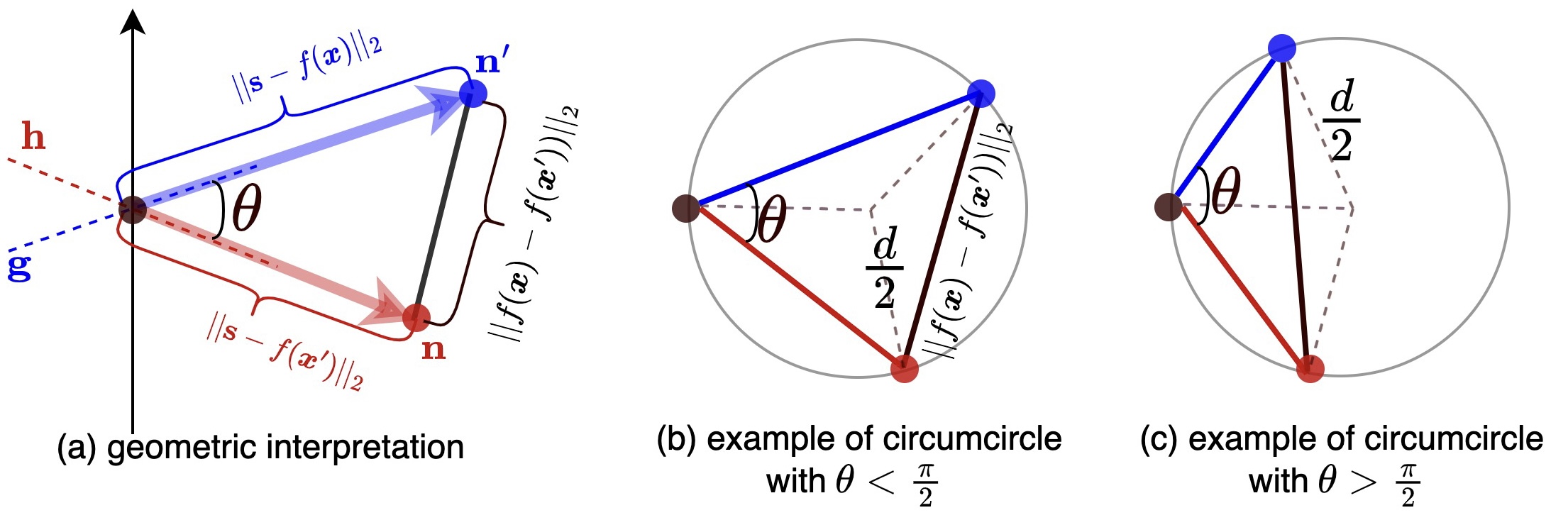
Figure 1: (a) Geometric interpretation of $|\rho_{1}|+|\rho_{2}|$. Circumcircles of the described triangle with (b) $\theta<\frac{\pi}{2}$ and (c) $\theta>\frac{\pi}{2}$.

It is well-known that the length of each edge of a triangle is upper bounded by the diameter of the circumscribed circle of the triangle. We show this fact in Figure 1(b) and Figure (c), where $\frac{d}{2}$ represents the radius of the circumcircle. According to the law of sine, we have $d=||f(\bm{x})-f(\bm{x}^{\prime})||_{2}\big{/}{sin(\theta)}$. Thus,

where the last inequality is because the query sensitivity on neighboring datasets is $\Delta_{2}f=\sup_{\bm{x}\sim\bm{x}^{\prime}}||f(\bm{x})-f(\bm{x}^{\prime})||_{2}$.

In (LABEL:eq:needs-to-show2), we have $(z_{1},z_{2},\mathbf{h},\mathbf{g})\in\mathcal{A}$, i.e., $\theta\in(\frac{\pi}{2}-\theta_{0},\frac{\pi}{2}+\theta_{0})$, $\theta_{0}\in[0,\frac{\pi}{2}]$. Thus, due to the symmetry of the sine function around $\frac{\pi}{2}$, we can obtain $\frac{2\Delta_{2}f}{sin(\theta)}\leq\frac{2\Delta_{2}f}{sin(\frac{\pi}{2}-\theta_{0})}=\frac{2\Delta_{2}f}{cos(\theta_{0})}$. As a result, we get $|\rho_{1}|+|\rho_{2}|\leq$ $||\mathbf{s}-f(\bm{x}^{\prime})||_{2}+||\mathbf{s}-f(\bm{x})||_{2}<\frac{2\Delta_{2}f}{cos(\theta_{0})}=2\Delta_{2}f\Big{/}\Big{(}\frac{\delta\Gamma(\frac{M-1}{2})}{\sqrt{\pi}\Gamma(\frac{M}{2})}\Big{)}^{\frac{1}{M-2}}$.

Finally, from (LABEL:eq:needs-to-show2), we can obtain the following sufficient condition for the R$1$SMG mechanism to achieve $(\epsilon,\delta)$-DP:

$$\mathrm{PLRV}^{(\mathbf{s})}_{(R1SMG(\bm{x})||R1SMG(\bm{x}^{\prime}))}$$

$$\leq \frac{1}{2\sigma_{*}}(|\rho_{1}|+|\rho_{2}|)^{2}\leq\frac{1}{2\sigma_{*}}\Big{(}2\Delta_{2}f\Big{/}\Big{(}\frac{\delta\Gamma(\frac{M-1}{2})}{\sqrt{\pi}\Gamma(\frac{M}{2})}\Big{)}^{\frac{1}{M-2}}\Big{)}^{2}\leq\epsilon,$$

which leads to $\sigma_{*}\geq\frac{2(\Delta_{2}f)^{2}}{\epsilon\psi}$. Moreover, due to the constraint of $P>2$ in Lemma 2, we require $M>2$ for the R1SMG mechanism. Thus, Theorem 5 follows. ∎

Implementation of R1SMG. According to the following theorem, we can obtain the desired random variable distributed on the Stiefel manifold by transforming samples drawn i.i.d. from standard Gaussian distribution.

Theorem 6.

[13, p. 29, Theorem 2.2.1] Let $\mathbf{x}\in\mathbb{R}^{M\times r}$, whose elements are i.i.d. Gaussian random variables from $\mathcal{N}(0,1)$. Then, $\mathbf{v}=\mathbf{x}(\mathbf{x}^{T}\mathbf{x})^{-1/2}$ is uniformly distributed on $\mathbb{V}_{r,M}$.

Thus, we can apply Theorem 6 with $r=1$ to draw the desired samples from $\mathbb{V}_{1,M}$. Then, applying (11), we can generate an instance of random noise for the R1SMG mechanism.

5.3 Expected Accuracy Loss Analysis

In this section, we investigate the expected accuracy loss of the R1SMG mechanism, i.e., $\mathbb{E}_{R1SMG}[\mathcal{L}]$. The results are summarized in Theorem 7.

Theorem 7.

For any fixed $\epsilon>0,0<\delta<1$, given a dataset $\bm{x}$ and a query result $f(\bm{x})\in\mathbb{R}^{M}$. We have $\mathbb{E}_{R1SMG}[\mathcal{L}]=||R1SMG(f(\bm{x}))-f(\bm{x})||_{2}^{2}=Tr[\bm{\Pi}]=\sigma_{*}\geq C_{R}(\Delta_{2}f)^{2}$, where $\sigma_{*}$ is the only nonzero eigenvalue of $\bm{\Pi}$, $C_{R}=\frac{2}{\epsilon\psi}$, and $\psi=\Big{(}\frac{\delta\Gamma(\frac{M-1}{2})}{\sqrt{\pi}\Gamma(\frac{M}{2})}\Big{)}^{\frac{2}{M-2}}$. $C_{R}$ has a decreasing trend as $M$ increases. When $M$ approaches infinity, $C_{R}$ converges to $\frac{2}{\epsilon}$ and $\mathbb{E}_{R1SMG}[\mathcal{L}]$ can be as low as $\frac{2(\Delta_{2}f)^{2}}{\epsilon}$.

Proof.

According to the noise generation process in R1SMG, i.e., (11), we have

$$\mathbb{E}_{R1SMG}[\mathcal{L}]=\mathbb{E}[||\mathbf{n}||_{2}^{2}]$$ (15)

$$= \mathbb{E}\Big{[}(\mathbf{v}\sigma_{*}^{1/2}z)^{T}\mathbf{v}\sigma_{*}^{1/2}z\Big{]}=\sigma_{*}\mathbb{E}[z^{2}]\stackrel{{\scriptstyle(a)}}{{=}}\sigma_{*}\stackrel{{\scriptstyle(b)}}{{\geq}}2(\Delta_{2}f)^{2}/(\epsilon\psi),$$

where (a) holds because $z^{2}\sim\chi^{2}(1)$, and (b) is due to Theorem 5. From (15), we also have $\mathbb{E}_{R1SMG}[\mathcal{L}]=\sigma_{*}=Tr[\bm{\Pi}]$.

To show the decreasing trend of $\mathbb{E}_{R1SMG}[\mathcal{L}]$ without dealing with the cumbersome notation of $\psi$, we use some intermediate results obtained in the proof of Theorem 5. To be more specific, we have $\psi=sin^{2}(\theta)$, where $\theta\in(\frac{\pi}{2}-\theta_{0},\frac{\pi}{2}+\theta_{0})$ is the angle between two instances of $M$-dimensional unit vectors, and $\theta_{0}=arccos\left(\left({\delta\Gamma(\frac{M-1}{2})}\big{/}{\sqrt{\pi}\Gamma(\frac{M}{2})}\right)^{1/(M-2)}\right)$. Cai et al. [7] has proved that when $M>2$, $\theta$ concentrates around $\frac{\pi}{2}$, and the concentration becomes stronger as the dimension $M$ grows. In particular, $\theta$ converges to $\frac{\pi}{2}$ at the rate of $\sqrt{M}$ when $M$ approaches infinity [7, p. 1840]. Thus, $\frac{1}{sin^{2}(\theta)}$ has a decreasing trend and converges to 1 due to the symmetry of sine function on $[0,\pi]$. Subsequently, we can have that $C_{R}=\frac{2}{\epsilon\psi}$ has a decreasing trend as well. In addition, when $M$ approaches infinity, we get that $C_{R}$ converges to $\frac{2}{\epsilon}$ and hence $\mathbb{E}_{R1SMG}[\mathcal{L}]$ can be as low as $\frac{2(\Delta_{2}f)^{2}}{\epsilon}$. ∎

Curse Lifted. (15) clearly shows that we have lifted the identified curse by considering noise attributed to a singular multivariate Gaussian distribution with rank-1 covariance matrix. In particular, the expected accuracy loss introduced by the R$1$SMG mechanism is $Tr[\bm{\Pi}]$, which equal to the only nonzero eigenvalue $\sigma_{*}$ but is not the summation of $M$ positive eigenvalues any more like in the existing Gaussian mechanisms.

From Theorem 4 and Theorem 7, we arrive at Corollary 1.

Corollary 1.

Compared with the classic Gaussian, analytic Gaussian, and MVG mechanisms, the R1SMG mechanism leads to expected accuracy loss on a much lower order with regard to the dimension of the query results $f(\bm{x})$. In particular, $C_{R}=\Theta(1)$ while $C_{C}=C_{A}=\Theta(M)$ for $f(\bm{x})\in\mathbb{R}^{M}$ and $C_{M}=\Theta(MN)$ for $f(\bm{x})\in\mathbb{R}^{M\times N}$.

Proof.

From Theorem 5, we have $\frac{1}{\psi}=\Big{(}\frac{\sqrt{\pi}\Gamma(\frac{M}{2})}{\delta\Gamma(\frac{M-1}{2})}\Big{)}^{\frac{2}{M-2}}=\exp\Big{(}\frac{2}{M-2}\ln\Big{(}\frac{\sqrt{\pi}\Gamma(\frac{M}{2})}{\delta\Gamma(\frac{M-1}{2})}\Big{)}\Big{)}.$ By connecting $\frac{\Gamma(\frac{M}{2})}{\Gamma(\frac{M-1}{2})}$ to the normalization constant of the Beta distribution $Beta(\alpha,\beta)$ with $\alpha=\frac{M-1}{2}$ and $\beta=\frac{1}{2}$, it gives $\Theta\Big{(}\frac{\Gamma(\frac{M}{2})}{\Gamma(\frac{M-1}{2})}\Big{)}=\Theta\left(\frac{\sqrt{M-2}}{\sqrt{2}}\right)$ [7]. As a result, we have $C_{R}=\frac{2}{\epsilon\psi}=\Theta(\frac{1}{\psi})=\Theta\left(\exp\left(\frac{2}{M-2}\ln\frac{\sqrt{M-2}}{\sqrt{2}}\right)\right)=\Theta(1)$. The results of $C_{C}$, $C_{A}$, and $C_{M}$ directly follow Theorem 4. Hence, we can easily observe that the expected accuracy loss of the R1SMG mechanism is on a much lower order than that of the classic Gaussian, of the analytic Gaussian, and of the MVG mechanisms. ∎

Moreover, in Appendix B, we plot the empirical $\mathbb{E}[\mathcal{L}]$ versus $M$ achieved by the R1SMG mechanism and by other mechanisms, respectively, and clearly show that $\mathbb{E}_{R1SMG}[\mathcal{L}]$ has a decreasing trend as $M$ increases and eventually converges, whereas all the other mechanisms result in expected accuracy loss increasing with $M$ (cf. Figure 8).

5.4 Discussion on Privacy Leakage of Utilizing Vector in the Null Space of $\mathbf{v}$

The R$1$SMG mechanism does not span the entire space of $\mathbb{R}^{M}$. Therefore, it may raise concerns about privacy leakage if one takes advantage of the vector in the null space of $\mathbf{v}$. In other words, let $\mathbf{s}$ be the output of R$1$SMG and $\mathbf{u}\in Null(\mathbf{v})=\{\mathbf{u}|<\mathbf{u},\mathbf{v}>=0\}$. Since $\mathbf{n}\in Span(\mathbf{v})$, one can have $<\mathbf{u},\mathbf{s}>=<\mathbf{u},f(\bm{x})+\mathbf{n}>=<\mathbf{u},f(\bm{x})>$, which implies potential privacy leakage of queries on $f(\bm{x})$.

However, we highlight that $\mathbf{v}$ is randomly sampled from $\mathcal{U}(\mathbb{V}_{1,M})$, which is an intermediate noise to produce the final noise of the R$1$SMG mechanism and will not be made public. Note that this is not against the core idea of DP, i.e., “privacy without obscurity", because the entire noise generation process, i.e, (11), including the choice of distribution parameters are transparent. Thus, the probability that a constructed $\mathbf{u}$ that is in the null space of a randomly sampled $\mathbf{v}$ is zero, i.e., $\Pr[\mathbf{u}\in Null(\mathbf{v})]=\frac{\mu(Null(\mathbf{v}))}{\mu(\mathbb{R}^{M})}=0$, where $\mu(\cdot)$ is the Lebesgue measure of a measurable set.

For better explanation, , we give toy examples in $\mathbb{R}^{2}$ and $\mathbb{R}^{3}$ (when $M=2$ and $M=3$). Note that in practice R1SMG requires $M>2$, here we use $\mathbb{R}^{2}$ just to visualize the idea (the probability that a constructed $\mathbf{u}$ that is in the null space of a randomly sampled $\mathbf{v}$ is zero) which is independent of the dimension. In $\mathbb{R}^{2}$, $\mathbb{V}_{1,2}$ is the unit circle shown in Figure 2 (left). Suppose that $\mathbf{v}_{1}=[-1/\sqrt{5},2/\sqrt{5}]^{T}$ is the randomly sampled variable in $\mathbb{V}_{1,2}$. Then $Null(\mathbf{v}_{1})$ is $\mathcal{I}$ (the dashed line orthogonal to $\mathbf{v}_{1}$). Clearly, the probability of sampling a point from $\mathbb{R}^{2}$ that resides on a specific line is 0. Likewise, in $\mathbb{R}^{3}$, $\mathbb{V}_{1,3}$ is the unit sphere shown in Figure 2 (right). Suppose that $\mathbf{v}_{2}=[1/\sqrt{3},-1/\sqrt{3},1/\sqrt{3}]^{T}$ is the randomly sampled variable in $\mathbb{V}_{1,3}$. Then $Null(\mathbf{v}_{2})$ is $\mathcal{F}$ (the plane orthogonal to $\mathbf{v}_{2}$). The probability of sampling a point from $\mathbb{R}^{3}$ that resides on a specific plane is also 0. Although, it is publicly known that $\mathbf{v}$ is sampled from $\mathcal{U}(\mathbb{V}_{1,M})$, the Lebesgue measure of $Null(\mathbf{v})$ (given $\mathbf{v}\subset\mathbb{V}_{1,M}$) is still 0. For example, the probability of sampling the blue points in Figure 2 (left) is 0, and the probability of sampling points residing on $\mathcal{C}\subset\mathcal{F}$ (the circle orthogonal to $\mathbf{v}_{2}$) in Figure 2 (right) is also 0. Hence, by generating $\mathbf{v}$ randomly, the R$1$SMG mechanism will cause privacy leakage of using the vectors in the null space of $\mathbf{v}$ to have probability zero.

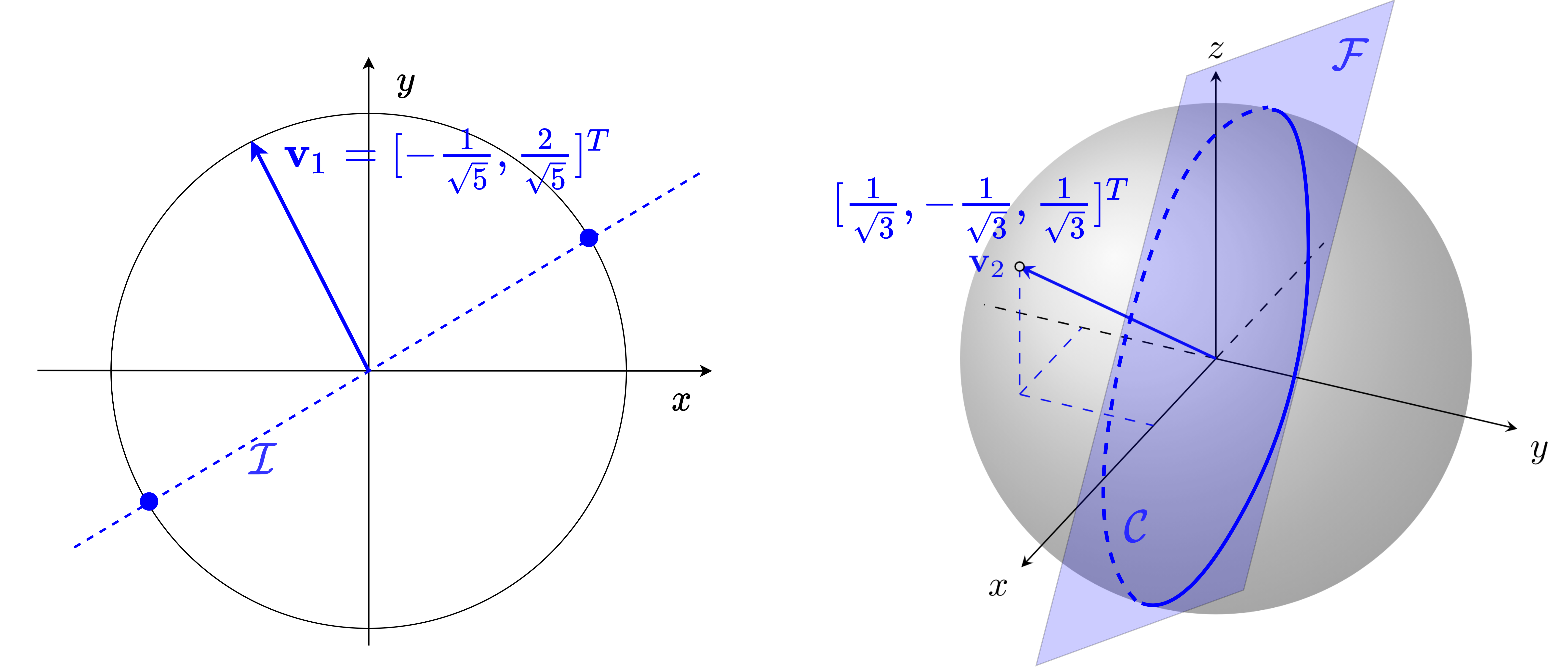
Figure 2: Visualization of the null space of the noise generated by the R$1$SMG mechanism. Left: $\mathbb{V}_{1,2}$. Right: $\mathbb{V}_{1,3}$.

6 Accuracy Stability

Now, we evaluate the accuracy stability achieved by various output perturbation DP mechanisms by studying the kurtosis and skewness of the distribution of $\mathcal{L}$ (the non-deterministic accuracy loss defined in Definition 1). In particular,

$\bullet$ Kurtosis, a descriptor of “tail extremity” of a probability distribution, is defined as the ratio between the $4$th moment and the square of the $2$nd moment of a random variable, i.e., $\frac{\mathbb{E}[\mathcal{L}^{4}]}{(\mathbb{E}[\mathcal{L}^{2}])^{2}}$. A larger kurtosis means that outliers or extreme large values are less likely to be generated in a given probability distribution [46].

$\bullet$ Skewness, a descriptor of the “bulk” of a probability distribution, is defined as the ratio between the $3$rd moment and the square root of the cube of the $2$nd moment of a random variable, i.e., $\frac{\mathbb{E}[\mathcal{L}^{3}]}{(\mathbb{E}[\mathcal{L}^{2}])^{3/2}}$. A larger skewness means that the bulk of the samples is at the left region of the PDF and the right tail is longer.

As a result, in order to have high accuracy stability on the perturbed query result, $\mathcal{L}$ with both larger kurtosis and skewness is preferred. We summarize the theoretical results for various mechanisms in Theorem 8 and Theorem 9.

Theorem 8.

The kurtosis of the distribution of $\mathcal{L}$ in the R1SMG mechanism is $\frac{35}{3}$ which is larger than that of the classic Gaussian mechanism, of the analytic Gaussian mechanism, and of the MVG mechanism, i.e., the PDF of $\mathcal{L}$ in the R1SMG mechanism is more leptokurtic than that in the classic Gaussian, in the analytic Gaussian, and in the MVG mechanism.

Proof.

First, for the proposed R1SMG, we have

$$\begin{aligned} &\leavevmode\resizebox{433.62pt}{}{${\rm{Kurt}_{R1SMG}}(\mathcal{L})=\frac{\mathbb{E}[\mathcal{L}^{4}]}{(\mathbb{E}[\mathcal{L}^{2}])^{2}}\stackrel{{\scriptstyle(a)}}{{=}}\frac{\mathbb{E}\left[\left((\mathbf{v}\sqrt{\sigma_{*}}z)^{T}\mathbf{v}\sqrt{\sigma_{*}}z\right)^{4}\right]}{\left(\mathbb{E}\left[\left((\mathbf{v}\sqrt{\sigma_{*}}z)^{T}\mathbf{v}\sqrt{\sigma_{*}}z\right)^{2}\right]\right)^{2}}=\frac{\mathbb{E}\left[(z\sigma_{*}z)^{4}\right]}{\left(\mathbb{E}\left[(z\sigma_{*}z)^{2}\right]\right)^{2}}$}\\ &\leavevmode\resizebox{346.89731pt}{}{$\stackrel{{\scriptstyle(b)}}{{=}}\frac{48\sigma_{*}^{4}+32\sigma_{*}^{3}\sigma_{*}+12(\sigma_{*}^{2})^{2}+12\sigma_{*}^{2}(\sigma_{*})^{2}+(\sigma_{*})^{4}}{\big{(}2\sigma_{*}^{2}+(\sigma_{*})^{2}\big{)}^{2}}=\frac{35}{3}$},\end{aligned}$$

where $(a)$ is due to the noise generation process of R1SMG in (11) and $(b)$ is obtained by applying Lemma 1 with $\mathbf{A}=1$ and $\bm{\Xi}=\sigma_{*}$ (i.e., the case of univariant Gaussian).

Then, we show that both classic Gaussian mechanism and the MVG mechanism will result in $\mathcal{L}$ with kurtosis less than $\frac{35}{3}$. In particular, the classic Gaussian mechanism (denoted as $\mathcal{G}$) adds i.i.d. noise to each entry of $f(\bm{x})$, $\mathbf{n}_{i}\sim\mathcal{N}(0,\sigma^{2}),i\in[1,M]$. Thus, we have $\mathbb{E}_{\mathcal{G}}[\mathcal{L}^{t}]=\mathbb{E}_{z_{i}\sim\mathcal{N}(0,1)}\left[\left(\sum_{i}\sigma^{2}z_{i}^{2}\right)^{t}\right]=\sigma^{2t}\mathbb{E}_{U\sim\chi^{2}(M)}[U^{t}]=\sigma^{2t}2^{t}\frac{\Gamma(t+\frac{M}{2})}{\Gamma(\frac{M}{2})}$, where the last equality follows from the $t$th moments of Chi-squared random variable. Set $t$ to be 4 and 2, one can verify that ${\rm{Kurt}_{\mathcal{G}}}(\mathcal{L})=\frac{\mathbb{E}_{\mathcal{G}}[\mathcal{L}^{4}]}{(\mathbb{E}_{\mathcal{G}}[\mathcal{L}^{2}])^{2}}={\sigma^{8}2^{4}\frac{\Gamma(4+\frac{M}{2})}{\Gamma(\frac{M}{2})}}\Big{/}{\Big{(}\sigma^{4}2^{2}\frac{\Gamma(2+\frac{M}{2})}{\Gamma(\frac{M}{2})}\Big{)}^{2}}<\frac{35}{3},\forall M>1.$

The same analysis holds for the analytic Gaussian mechanism, as it adds i.i.d. Gaussian noise with variance $\sigma_{A}^{2}$.

MVG introduces the matrix-valued noise attributed to a matrix-valued Gaussian distribution, i.e., $\mathcal{N}(\mathbf{0},\bm{\Sigma},\bm{\Psi})$, and the vectorization of the noise matrix is also attributed to a multivariate Gaussian distribution, i.e., $\mathcal{N}(\mathbf{0},\bm{\Sigma}\otimes\bm{\Psi})$ [21]. Denote $\bm{\Xi}=\bm{\Sigma}\otimes\bm{\Psi}$, and let $k>1$ be an integer, we first have

$$\begin{aligned} &(Tr[\bm{\Xi}])^{k}=(Tr[\bm{\Sigma}\otimes\bm{\Psi}])^{k}=\left[\left(\sum_{i=1}^{{\rm{rank}}(\bm{\Sigma})}\sigma_{i}(\bm{\Sigma})\right)\left(\sum_{j=1}^{{\rm{rank}}(\bm{\Psi})}\sigma_{j}(\bm{\Psi})\right)\right]^{k}\\ >&\sum_{i=1,j=1}^{{\rm{rank}}(\bm{\Sigma}),{\rm{rank}}(\bm{\Psi})}\big{(}\sigma_{i}(\bm{\Sigma})\sigma_{j}(\bm{\Psi})\big{)}^{k}=Tr\left[(\bm{\Sigma}\otimes\bm{\Psi})^{k}\right]=Tr\left[\bm{\Xi}^{k}\right].\end{aligned}$$

Similarly, for any positive integer $k_{1}>k_{2}\geq 1$ and symmetric $\bm{\Xi}\in\mathbb{PD}$, we have

$$Tr[\bm{\Xi}^{k_{1}}](Tr[\bm{\Xi}])^{k_{2}}>Tr[\bm{\Xi}^{k_{1}}]Tr[\bm{\Xi}^{k_{2}}]$$

$$= \left(\sum_{i=1}^{{\rm{rank}}(\bm{\Xi})}(\sigma_{i}(\bm{\Xi}))^{k_{1}}\right)\left(\sum_{i=1}^{{\rm{rank}}(\bm{\Xi})}(\sigma_{i}(\bm{\Xi}))^{k_{2}}\right)>\sum_{i=1}^{{\rm{rank}}(\bm{\Xi})}(\sigma_{i}(\bm{\Xi}))^{k_{1}+k_{2}}$$

$$= Tr[\bm{\Xi}^{k_{1}+k_{2}}].$$

Then, according to Lemma 1, we have

$$\begin{aligned} &{\rm{Kurt}_{MVG}}(\mathcal{L})=\frac{\mathbb{E}[\mathcal{L}^{4}]}{(\mathbb{E}[\mathcal{L}^{2}])^{2}}=\frac{\mathbb{E}[(\mathbf{n}^{T}\mathbf{n})^{4}]}{(\mathbb{E}[(\mathbf{n}^{T}\mathbf{n})^{2}])^{2}}=\frac{\mathbb{E}[Q(\mathbf{n})^{4}]}{(\mathbb{E}[Q(\mathbf{n})^{2}])^{2}}\\ =&\leavevmode\resizebox{411.93767pt}{}{$\frac{48Tr[\bm{\Xi}^{4}]+32Tr[\bm{\Xi}^{3}]Tr[\bm{\Xi}]+12(Tr[\bm{\Xi}^{2}])^{2}+12Tr[\bm{\Xi}^{2}](Tr[\bm{\Xi}])^{2}+(Tr[\bm{\Xi}])^{4}}{\big{(}2Tr[\bm{\Xi}^{2}]+(Tr[\bm{\Xi}])^{2}\big{)}^{2}}$}.\end{aligned}$$

Next, we can obtain

$48Tr[\bm{\Xi}^{4}]<\frac{104}{3}(Tr[\bm{\Xi}^{2}])^{2}+\frac{8}{3}Tr[\bm{\Xi}^{2}](Tr[\bm{\Xi}])^{2}+\frac{32}{3}(Tr[\bm{\Xi}])^{4}$

and $32Tr[\bm{\Xi}^{3}]Tr[\bm{\Xi}]<32Tr[\bm{\Xi}^{2}](Tr[\bm{\Xi}])^{2}$. Thus, we get ${\rm{Kurt}_{MVG}}(\mathcal{L})<\frac{\frac{35}{3}\left(4Tr[\bm{\Xi}^{2}]+4Tr[\bm{\Xi}^{2}](Tr[\bm{\Xi}])^{2}+(Tr[\bm{\Xi}])^{4}\right)}{4Tr[\bm{\Xi}^{2}]+4Tr[\bm{\Xi}^{2}](Tr[\bm{\Xi}])^{2}+(Tr[\bm{\Xi}])^{4}}=\frac{35}{3}$ , which concludes the proof. ∎

Theorem 9.

The skewness of the distribution of $\mathcal{L}$ in the R1SMG mechanism is $\frac{5\sqrt{3}}{3}$ which is larger than that of the classic Gaussian mechanism, of the analytic Gaussian mechanism, and of the MVG mechanism, i.e., the PDF of $\mathcal{L}$ in the R1SMG mechanism is more right-skewed than that in the classic Gaussian, in the analytic Gaussian, and in the MVG mechanism.

Proof.

The proof follows the same procedure as the proof of Theorem 8, thus we only show the key steps here.

For the proposed R1SMG, we have ${\rm{skew}_{\mathrm{R1SMG}}}(\mathcal{L})=\frac{\mathbb{E}[\mathcal{L}^{3}]}{(\mathbb{E}[\mathcal{L}^{2}])^{3/2}}=\frac{\mathbb{E}\left[(z\sigma_{*}z)^{3}\right]}{\left(\mathbb{E}\left[(z\sigma_{*}z)^{2}\right]\right)^{3/2}}=\frac{\sigma_{*}^{3}2^{3}\frac{\Gamma(3+\frac{1}{2})}{\Gamma(\frac{1}{2})}}{\left(\sigma_{*}^{2}2^{2}\frac{\Gamma(2+\frac{1}{2})}{\Gamma(\frac{1}{2})}\right)^{3/2}}=\frac{5\sqrt{3}}{3}.$

For the classic Gaussian mechanism, one can verify that
${\rm{skew}_{\mathcal{G}}}(\mathcal{L})=\frac{\sigma_{G}^{6}2^{3}\frac{\Gamma(3+\frac{M}{2})}{\Gamma(\frac{M}{2})}}{\left(\sigma_{G}^{4}2^{2}\frac{\Gamma(2+\frac{M}{2})}{\Gamma(\frac{M}{2})}\right)^{3/2}}=\frac{\frac{\Gamma(3+\frac{M}{2})}{\Gamma(\frac{M}{2})}}{\left(\frac{\Gamma(2+\frac{M}{2})}{\Gamma(\frac{M}{2})}\right)^{3/2}}<\frac{5\sqrt{3}}{3},\forall M>1$.

The same analysis holds for the analytic Gaussian mechanism, as it adds i.i.d. Gaussian noise with variance $\sigma_{A}^{2}$.

For the MVG mechanism, it is easy to check that
${\rm{skew}_{MVG}}(\mathcal{L})=\frac{\mathbb{E}[\mathcal{L}^{3}]}{(\mathbb{E}[\mathcal{L}^{2}])^{3/2}}=\frac{\mathbb{E}[(\mathbf{n}^{T}\mathbf{n})^{3}]}{(\mathbb{E}[(\mathbf{n}^{T}\mathbf{n})^{2}])^{3/2}}=\frac{\big{(}8Tr[\bm{\Xi}^{3}]+6Tr[\bm{\Xi}^{2}]Tr[\bm{\Xi}]+(Tr[\bm{\Xi}])^{3}\big{)}}{\big{(}2Tr[\bm{\Xi}^{2}]+(Tr[\bm{\Xi}])^{2}\big{)}^{3/2}}$, $\bm{\Xi}=\bm{\Sigma}\otimes\bm{\Psi}$. Besides, we have shown that for any positive integer $k$, $k_{1}$, and $k_{2}$, we have $(Tr[\bm{\Xi}])^{k}>Tr[\bm{\Xi}^{k}]$ and $Tr[\bm{\Xi}^{k_{1}}](Tr[\bm{\Xi}])^{k_{2}}>Tr[\bm{\Xi}^{k_{1}+k_{2}}]$. Thus, one can check that $({\rm{skew}_{MVG}}(\mathcal{L}))^{2}=\frac{\big{(}8Tr[\bm{\Xi}^{3}]+6Tr[\bm{\Xi}^{2}]Tr[\bm{\Xi}]+(Tr[\bm{\Xi}])^{3}\big{)}^{2}}{\big{(}2Tr[\bm{\Xi}^{2}]+(Tr[\bm{\Xi}])^{2}\big{)}^{3}}<\frac{\frac{25}{3}\big{(}2Tr[\bm{\Xi}^{2}]+(Tr[\bm{\Xi}])^{2}\big{)}^{3}}{\big{(}2Tr[\bm{\Xi}^{2}]+(Tr[\bm{\Xi}])^{2}\big{)}^{3}}$, i.e., ${\rm{skew}_{MVG}}(\mathcal{L})<\frac{5\sqrt{3}}{3}$. ∎

Remark 1.

We can consider the univariate Gaussian with unit covariance, i.e., $\mathcal{N}(\mu,1)$, as a reference distribution, whose kurtosis value and skewness value are $3$ and $0$, respectively. Then, it suggests that the distribution of $\mathcal{L}$ in the R1SMG mechanism are much more leptokurtic and right-skewed than $\mathcal{N}(\mu,1)$. Moreover, since the noise used in the classic Gaussian, analytic Gaussian, and MVG mechanisms are characterized by full-rank covariance matrices, their kurtosis values and skewness values asymptotically converge to $3+12/H$ and $\sqrt{8/H}$, respectively [26] ($H$ is the degree of freedom of the obtained $\mathcal{L}$, and $H=M$ for $f(\bm{x})\in\mathbb{R}^{M}$). It means that the distributions of $\mathcal{L}$ in the Gaussian mechanism and MVG are similar to $\mathcal{N}(\mu,1)$ when $M$ is large.

In Section 7.1, by using 2D count query as an example, we will empirically show that the distribution of $\mathcal{L}$ obtained in the R1SMG mechanism is more leptokurtic and right-skewed than those of the classic Gaussian, the analytic Gaussian, and the MVG mechanisms (cf. Figure 4). In other words, the R1SMG mechanism can provide differentially private query results with the highest accuracy stability.

Based on the above theoretical analysis, we can have the following corollary.

Corollary 2.

The R1SMG mechanism outperforms the classic Gaussian, the analytic Gaussian, and the MVG mechanism, because it boosts the utility of the query results by achieving lower expected accuracy loss and higher accuracy stability.

7 Experiments

In this section, we conduct three case studies to validate the utility boosting achieved by the R1SMG mechanism, i.e., 2D count query, principal component analysis (PCA), and deep learning, all in a differentially private manner. The query results of these case studies are either matrices or tensors, so the R1SMG, classic Gaussian, and analytic Gaussian mechanisms will first generate noise in vector form, and then reshape the noise into the forms required by different studies.

7.1 Case Study i@: Uber Pickup Count Query

In this case study, we utilize the New York City (NYC) Uber pickups dataset [2], on which we are interested in releasing the counts of Uber pickups in different areas of NYC from “4/1/2014 00:11:00” to “4/3/2014 23:57:00” in a differentially private manner. The size of the count query $f(\bm{x})$ is determined by the partition areas (defined later) of NYC. Location and trajectory privacy breaches have been reported and investigated in several research works [33, 47, 24, 36]. Thus, it is important to guarantee that the existence or absence of any pickup record is private when sharing the count query.

In particular, we partition the map of NYC into small areas by evenly dividing the latitude and longitude into 89 disjoint intervals. As a result, the considered query is $f(\bm{x})\in\mathbb{R}^{89\times 89}$, whose entries record the number of Uber pickups in different small areas. The sensitivity of this query is 2, because the absence or presence of a specific pickup can change at most 2 entries of $f(\bm{x})$ by 1. We also consider that the data consumer (i.e., the query result recipient) has the prior knowledge of the valid pickup areas in the resulted $89\times 89$ small areas. Thus, he can perform post-processing on the noisy count query to eliminate the values in invalid areas (e.g., it is impossible to have Uber pickups over the Hudson River). We visualize the non-private Uber pickup count query in Figure 3(a). We observe high volumes of pickups around Soho, Fifth avenue, and LaGuardia Airport.

(a) Non-private	(b) R1SMG
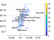
(c) classic Gauss.	(d) Analytic Gauss.
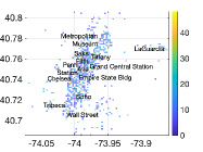
(e) MVG	(f) MGM
(g) DAWA	(h) $H_{b}$

Figure 3: Visualization of (a) non-private counts, (b)-(h) are differentially private 2D counts obtained by the R1SMG, classic Gaussian, analytic Gaussian, MVG, MGM, DAWA, and $H_{b}$ mechanisms, respectively.

Comparisons with Mechanisms. In additional to the $(\epsilon,\delta)$-DP output perturbation mechanisms, i.e., the classic Gaussian, analytic Gaussian, MVG, and MGM ([48] a variant of MVG) mechanisms, we also compare the R1SMG mechanism with the mechanisms that are specially developed for differentially private 2D count queries. In particular, they are (i) DAWA [32], which obtains differentially private count queries by adding noise that is adapted to both the input data and the given query set, and (ii) $H_{b}$ [39], which answers range queries using noisy hierarchies of equi-width histograms.

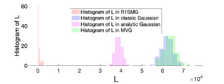
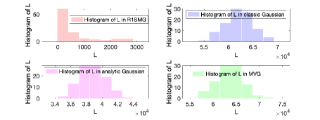
(a) Histogram of $\mathcal{L}$ for various mechanisms	(b) Histogram of $\mathcal{L}$ (zoomed in)
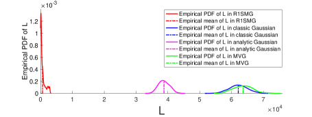
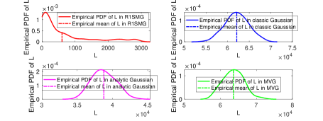
(c) Empirical PDF and mean of $\mathcal{L}$ for various mechanisms	(d) Empirical PDF and mean of $\mathcal{L}$ (zoomed in)

Figure 4: Accuracy loss introduced by different output perturbation mechanisms when $\epsilon=0.5$ and $\delta=10^{-7}$.

Results. We visualize the differential-privately released count queries obtained by the R1SMG and other comparing mechanisms in Figures 3(b)-(h). The privacy budgets for all considered mechanismsm are $\epsilon=0.5$ and $\delta=10^{-7}$. Clearly, the R1SMG mechanism outperforms all the comparing output perturbation mechanisms (i.e., Figure 3(c)-(f)), as it preserves the global and local patterns of the non-private count query in Figure 3(a) in the best way. In contrast, the classic Gaussian, MVG, and MGM mechanisms greatly compromise the utility of the count query results. For example, in Figures 3(c), (e), and (f) many areas on the Manhattan island have no pickup counts, and the maximum count is also increased significantly (i.e., higher than 60, 50, and 40, respectively, compared to the non-private maximum count which is only 25). Although the analytic Gaussian mechanism outperforms the classic Gaussian and MVG mechanisms by calibrating the noise variance exactly, it still introduces noise with higher magnitude than the R1SMG mechanism. Finally, we observe that the R1SMG mechanism has comparable performance with DAWA and $H_{b}$ that are developed specially for differentially private range queries. The error over ground truth ratios, i.e., $||\mathcal{M}(f(\bm{x}))-f(\bm{x})||_{F}/||f(\bm{x})||_{F}$ ($\mathcal{M}$ stands for a general mechanism), introduced by the R1SMG, DAWA, and $H_{b}$ mechanisms are $0.47\%$, $0.43\%$, and $0.72\%$, respectively. Note that DAWA has slightly better results because it is data-dependent (the noise is customized to the input data [32]), and that $H_{b}$ has even worse results although it adopts “constrained inference” (an accuracy boosting scheme) to control the mean square error of counting queries at various granularities. Moreover, not only does the R1SMG mechanism introduces comparable errors with those by the two task-specific mechanisms under the same privacy guarantee, but also it is very promising in other real-world tasks because it is not task-dependent.

Utility boosting and stability. Next, we empirically corroborate that the R1SMG mechanism boosts the utility of the NYC Uber pickup count query by achieving lower accuracy loss and higher accuracy stability. Specifically, by setting $\epsilon=0.5$ and $\delta=10^{-7}$, we repeat the noise generation process 100 times for the R1SMG, classic Gaussian, analytic Gaussian, and MVG mechanisms, respectively, and calculate the accuracy loss (i.e., $\mathcal{L}$, in Definition 1). In Figure 4, we plot the corresponding histograms, empirical average values of $\mathcal{L}$, and the empirical PDFs, obtained by different mechanisms. In particular, Figure 4(a) plots the histograms of $\mathcal{L}$ for various mechanisms on the same $x$-axis, and Figure 4(b) is the zoomed in histograms for each mechanism. Figure 4(c) demonstrates the empirical PDF and mean of $\mathcal{L}$ for each mechanism on the same $x$-axis, and Figure 4(d) shows the corresponding zoomed in plots.

Figure 4 shows that the empirical mean accuracy loss obtained by using the R1SMG mechanism is less than those obtained by the other mechanisms. This means that under the same privacy guarantee, the R1SMG mechanism introduces additive noise with the least amount of magnitude (squared Frobenius norm), which lead to lower empirical accuracy loss. In particular, $\mathcal{L}$ obtained by the R1SMG mechanism is on the order of $10^{3}$, whereas, $\mathcal{L}$ obtained by the other mechanisms is in the order of $10^{4}$. We can also find that the histogram and the empirical PDF of $\mathcal{L}$ obtained by the R1SMG mechanism are much more leptokurtic and right-skewed than those achieved by the others. In particular, compared with those obtained by the other mechanisms that have bell shapes, the empirical PDF of $\mathcal{L}$ achieved by the R1SMG mechanism has a longer and fatter tail, a higher and sharper central peak, and the density is more densely distributed on the left side. The results corroborate the analysis in Remark 1. Thus, for a given $(\epsilon,\delta)$-DP requirement, it is less likely for the R1SMG mechanism to generate additive noise with large magnitude.

7.2 Case Study ii@: PCA

In this case study, we explore differentially private principal component analysis (PCA) using the Swarm Behaviour dataset [1]. It contains 24016 records of flocking behaviour (i.e., the way that groups of birds, insects, fish or other animals, move close to each other). Each record has 2400 features characterizing a flocking observation, e.g., radius of separation of groups of insects, moving direction, moving velocity, etc. Each data record is assigned a binary label, and “1" represents “flocking behavior" and “0" represents “not flocking". The values of all features are normalized between $-1$ and $1$. Similar to [11], we consider the query $f(\bm{x})$ as the covariance matrix of this dataset, i.e., $f(\bm{x})={D^{T}D}/{24016}\in\mathbb{R}^{2400\times 2400}$, where $D\in\mathbb{R}^{24016\times 2400}$ denotes the considered Swarm Behaviour data. Then, the $l_{2}$ sensitivity of the query function is $s_{2}(f)=\sup_{D_{1},D_{2}}\frac{||{D_{1}}(i)^{T}{D_{1}}(i)-{D_{2}}(i)^{T}{D_{2}}(i)||_{F}}{24016}=\frac{\sqrt{2\times 2400^{2}}}{24016}=\frac{2400\sqrt{2}}{24016}$ (cf. Appendix B of [11]), where $D_{1}$ and $D_{2}$ are two neighboring Swarm Behavior datasets, the first equality is obtained by assuming that the only different sensor record is at the $i$th row of $D_{1}$ and $D_{2}$, i.e., ${D_{1}}(i)$ and ${D_{2}}(i)$, and the second equality is because a single observation can change all $2400^{2}$ entries of $D^{T}D$ by 2 at most.

We conduct singular value decomposition on the queried result (i.e., the noisy empirical covariance matrix) to extract the components of the dataset. The considered evaluation metric is the total deviation which is defined as $\Delta=\textstyle\sum_{i=1}^{2041}\Delta_{i}=\textstyle\sum_{i=1}^{2041}|\lambda_{i}-\widetilde{\mathbf{v}_{i}}^{T}\mathbf{C}\widetilde{\mathbf{v}_{i}}|$, where $\mathbf{C}$ is the ground-truth (non-private) empirical covariance matrix, $\lambda_{i}$ is the $i$th eigenvalue of $\mathbf{C}$, and $\widetilde{\mathbf{v}_{i}}$ is the $i$th differentially private component (eigenvector). Specifically, $\Delta_{i}$ quantifies the deviation of the variance from $\lambda_{i}$ in the direction of the $i$th component. The smaller $\Delta$ is, the higher utility the obtained components have, and we have $\Delta=0$ for the non-private baseline.

Since PCA usually serves as a precursor to classification task, we also evaluate the utility of the queried data by projecting the dataset onto the subspace spanned by the first 20 PCs obtained from various noisy covariance matrices, and then measure the classification accuracy using the projected data. The higher the classification accuracy, the higher the utility of the perturbed covariance matrix. In the experiments, we use $60\%$ and $40\%$ of the dataset for training and testing, respectively, and the classification algorithm is the linear SVM. Note that the accuracy of the non-private baseline (i.e., classification using the original dataset project onto the first 20 PCs of the original covariance matrix) is $96.89\%$.

Comparisons with other Mechanisms. In addition to the output perturbation mechanisms, we also consider the principal components obtained from 3 task-specific differentially private algorithms designed specially for PCA, i.e., (i) PPCA [12], which generates privacy-preserving components by sampling orthonormal matrices from the matrix Bingham distribution parametermized by the original non-private empirical covariance matrix scaled by the privacy budget, (ii) MOD-SULQ [12], which directly perturbs the covariance matrix using calibrated Gaussian noise, and (iii) the Wishart mechanism [25], which perturbs the empirical covariance matrices using noise attributed to the Wishart distribution.

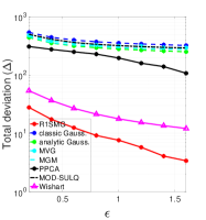
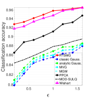
(a) Deviation versus $\epsilon$.	(b) Accuracy versus $\epsilon$.

Figure 5: Utility of the noisy covariance matrices obtained by various mechanisms. (a) The total deviation. (b) The classification accuracy measured on the projected testing dataset.

Results. In this experiment, we vary $\epsilon$ from $0.2$ to $1.6$ and set $\delta=10^{-7}$. Figure 5(a) and (b) plots the total derivation ($\Delta$) and classification accuracy on the projected testing data obtained from all mechanisms. Clearly, the R1SMG mechanism has the highest utility given various privacy budgets and is also the closest to the non-private baselines (i.e., $\Delta=0$ and $96.89\%$ accuracy). This is because the R1SMG mechanism introduces perturbation noise with much smaller magnitudes under the same privacy guarantee, compared with the other mechanisms. Taking the MVG mechanism for example, according to Theorem 3, when $\epsilon=1.6$ and $\delta=10^{-7}$, MVG requires $||\sigma(\bm{\Sigma}^{-1})||_{2}||\sigma(\bm{\Psi}^{-1})||_{2}\leq 0.011$ to achieve the desired privacy guarantee. This means that the covariance matrices will have very large singular values, which implies large expected accuracy loss (as discussed in Section 3) and causes the original data be overwhelmed by the additive noise. In fact, according to [11], for the MVG mechanism to have a decent performance on differentially private PCA, it requires $\epsilon\geq 5$. Moreover, in this case study, the R1SMG mechanism even outperforms the task-specific mechanisms including PPCA, MOD-SULQ, and Wishart. In other words, the R1SMG mechanism not only achieves the lowest $\Delta$, but also gives the highest classification accuracy for all the chosen $\epsilon$. This suggests that it is very promising in boosting the accuracy of high-dimensional differentially private query. Note that in this study, the R1SMG mechanism also achieves the most stable accuracy, i.e., the accuracy loss introduced by it has leptokurtic and right-skewed histogram and empirical PDF, but the others still have bell-shaped empirical PDFs (similar to Figure 4). We omit the plots due to space limit.

7.3 Case Study iii@: Deep Learning with DP

In this case study, we show the feasibility of replacing the classic Gaussian mechanism with the R1SMG in the DPSGD (differentially private stochastic gradient descent) optimization framework [3], and demonstrate that R1SMG can boost the utility (testing accuracy) of a differentially-private deep learning model and improve its training efficiency by reducing the number of epochs.

As a proof of concept, we consider the MNIST [31] and CIFAR-10 [29] dataset, and compare our R1SMG-based DPSGD with the seminal work of DPSGD in deep learning (Abadi et al. CCS’16 [3]). For a given deep neural network, Abadi et al. introduce calibrated i.i.d. Gaussian noise ($\mathcal{N}(\mathbf{0},\sigma^{2}C^{2}\mathbf{I})$) to the gradients computed on grouped batches of training data, where $C$ is a norm clipping parameter to control the sensitivity (Algorithm 1 in [3]). They also developed the privacy accountant scheme to tightly bound the cumulative privacy loss for the entire training process. In particular, the total privacy budget $(\epsilon,\delta)$ is determined by noise level $\sigma$, sampling ratio $q$, and the number of epochs $E$ (so number of gradient descent steps is $T=E/q$).

In the experiment, we give our R1SMG-based DPSGD the same total privacy budget $(\epsilon,\delta)$, $C$, $q$, and $E$ as those of DPSGA in [3]. Then, we amortize $(\epsilon,\delta)$ to all gradient descent steps in our R1SMG-based DPSGD, i.e., each step is assigned with $(\epsilon_{0},\delta_{0})$. To be more specific, $(\epsilon_{0},\delta_{0})$ is obtained by solving the following equations formulated using the strong composition theorem [19] considering $\frac{E}{q}$ repetitive executions of gradient descent.

$$\begin{cases}&\epsilon=\sqrt{2\frac{E}{q}\ln\left(\frac{1}{\delta^{\prime}}\right)}(q\epsilon_{0})+\frac{E}{q}(q\epsilon_{0})\left(e^{(q\epsilon_{0})}-1\right)\\ &\delta=\frac{E}{q}(q\delta_{0})+\delta^{\prime}\end{cases},$$ (16)

where $q\epsilon_{0}$ and $q\delta_{0}$ are due to privacy amplification via sampling [6, 27] (see discussion on page 3, right column of [3]). For example, based on the TensorFlow tutorial for DPSGD on MNIST [37], when $C=1$, $\sigma=1.1$, $q=\frac{256}{60000}$, and $E=30$, it leads to $\epsilon=1.795$. Then, setting $\delta=10^{-5}$, $\delta^{\prime}=10^{-10}$ and solving (16), we have $(\epsilon_{0},\delta_{0})=(0.71,3.33\times 10^{-7})$. When $C=1$, $\sigma=0.5$, $q=\frac{256}{60000}$, and $E=30$, it leads to $(16.983,10^{-5})$-DP for DPSGD, which makes $(\epsilon_{0},\delta_{0})=(5.42,3.33\times 10^{-7})$ for each gradient descent step in our R1SMG-based DPSGD.

Note that using strong composition theorem to assign amortized privacy budget to each step of our R1SMG-based DPSGD gives more favor to the classic Gaussian mechanism based DPSGD in the comparison. This is because strong composition is much looser than the privacy accountant scheme used in DPSGD (empirically validated by Figure 2 of [3]). Thus, the amortized $(\epsilon_{0},\delta_{0})$ can be limited. Developing a tight composition framework for the R1SMG mechanism in SGD-based learning will be a separate research topic.

Even though the original DPSGD is given more favor in the comparison, our R1SMG-based DPSGD still outperforms it by achieving higher training and testing accuracy. We first show the comparison results on MNIST using the above parameters setups in Figure 6. In particular, Figure 6(a) and (b) show the training and testing accuracy on MNIST for the first 30 epochs achieved by various approaches when the entire learning process is $(1.795,10^{-5})$-DP and $(16.983,10^{-5})$-DP (parameters discussed above), respectively. The blue lines and dashed lines in Figure 6 are the result of non-private SGD (the one uses original gradients calculated from the data).

(a) The entire process	(b) The entire process
is $(1.795,10^{-5})$-DP.	is $(16.983,10^{-5})$-DP.

Figure 6: Training and testing acc. on MNIST.

Compared with DPSGD, R1SMG-based DPSGD achieves higher training and testing accuracy in just a few epochs for the MNIST dataset. For example, when the total privacy budget is $(16.983,10^{-5})$, our method achieves 95% accuracy on the testing dataset using 5 epochs, whereas DPSGD requires 14 epochs. Our R1SMG-based DPSGD also leads to performance that is closer to the non-private baseline, because even though the amortized privacy budget for each R1SMG-based DPSGD step is limited, the magnitude of the perturbation noise introduced by the R1SMG mechanism is much less than that required by the classic Gaussian in DPSGD.

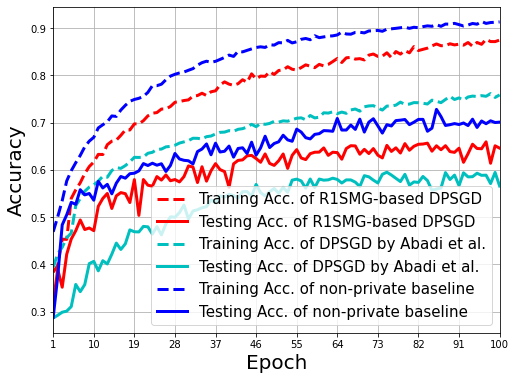
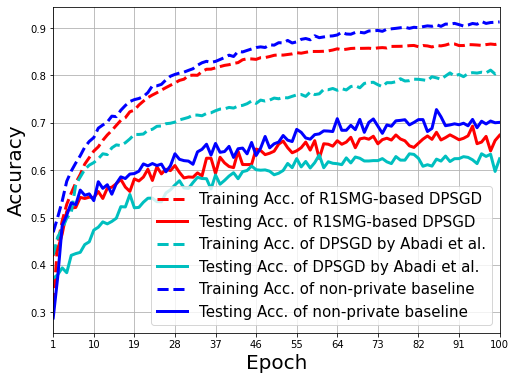
(a) The entire process	(b) The entire process
is $(2.673,10^{-5})$-DP.	is $(20.713,10^{-5})$-DP.

Figure 7: Training and testing acc. on CIFAR-10.

Then, we conduct the experiments on CIFAR-10 dataset with the same parameter setups while using 100 epochs, i.e., $E=100$. We also adopt the network architecture from the TensorFlow CNN tutorial [45]. The privacy budget for each step of R1SMG-based DPSGD, i.e., $(\epsilon_{0},\delta_{0})$ is also decided by solving (16) numerically. In particular, when $\sigma=1.1$ and $\sigma=0.5$, the entire process of DPSGD is $(2.673,10^{-5})$-DP and $(20.713,10^{-5})$-DP, respectively, which make $(\epsilon_{0},\delta_{0})$ become $(0.54,10^{-7})$ and $(3.52,10^{-7})$, respectively, for R1SMG-based DPSGD. The comparison results are shown in Figure 7. Clearly, our R1SMG-based DPSGD still outperforms DPSGD, i.e., both training and testing accuracy achieved by R1SMG-based DPSGD are closer to the non-private baselines compared with those achieved by DPSGD. In particular, R1SMG-based DPSGD improve the training efficiency by achieving a higher training accuracy (e.g., $>80\%$) in much fewer epochs compared with the original DPSGD.

8 Related Work

Many works have attempted to improve the classic Gaussian mechanism. Here, we review some representative ones.

The analytic Gaussian mechanism proposed by Balle et al. [5] (see Theorem 2) improves the classic Gaussian mechanism by calibrating the variance of the Gaussian noise directly using the Gaussian cumulative density function instead of the tail bound approximation, and develop an analytical solution to the variance given specific choices $\epsilon$ and $\delta$. Although this mechanism can reduce the magnitude of the noise when perturbing a scalar-valued quantity, it still suffers the curse of full-rank covariance matrices when applied to perturb high-dimensional query result (as discussed in Section 3).

Zhao et al. [49] investigate the classic Gaussian mechanism under high privacy budgets, i.e., $\epsilon>1$, and derive a closed-form upper bounds for the noise variance used in the analytic Gaussian mechanism. Their mechanism can achieve utility higher than the classic Gaussian mechanisms, but still lower than the analytic Gaussian mechanism.

Chanyaswad et al. [11] (see Definition 4 and Theorem 3) propose the MVG mechanism and develop the technique of directional noise to restrict the impact of the perturbation noise on the utility of a matrix-valued query function. However, to obtain the directional noise, one either needs a domain expert to determine the principal components of the queried data or has to calculate them via principal component analysis which consumes some privacy budget.

Some other variants of the classic Gaussian mechanism includes the Generalized Gaussian mechanism [34], which investigates noise calibration under the general $l_{p}$ sensitivity, and the discrete Gaussian mechanism [9], which uses noise attributed to discrete Gaussian distribution to protect the privacy of query results in a discrete domain.

Our proposed R1SMG mechanism differs with the above mechanisms, as we explicitly require the covariance matrix of the additive noise to be rank-1. Thus, the R1SMG mechanism lifts the identified curse and boosts the utility of query results leading to guaranteed DP at much lower cost of accuracy loss.

9 Conclusions

In this paper, we have developed a novel DP mechanism, i.e., R1SMG, to boost the utility and stability of differentially-private query results. In particular, we first identify the curse of full-rank covariance matrices in all existing Gaussian-based DP mechanisms. Then, we lift the curse by developing R1SMG which perturbs the query results using noise that follows a singular multivariate Gaussian distribution with a random rank-1 covariance matrix. We rigorously analyze the privacy guarantee of the R1SMG mechanism, and theoretically demonstrate that it can achieve much lower accuracy loss and much higher accuracy stability than the classic Gaussian, analytic Gaussian, and the MVG mechanisms.

Appendix A Proof of (e) in Equation (5)

Define $\sigma(\bm{\Sigma})\stackrel{{\scriptstyle\text{def}}}{{=}}[a_{1},a_{2},\ldots,a_{M}]$ and $\sigma(\bm{\Psi})\stackrel{{\scriptstyle\text{def}}}{{=}}[b_{1},b_{2},\ldots,b_{N}]$. Since $\bm{\Sigma},\bm{\Psi}\in\mathbb{PD}$ and they are both symmetric, we have $a_{m}>0,\forall m\in[1,M]$ and $b_{n}>0,\forall n\in[1,N]$. Then, to prove (e) in (5), we essentially need to show that

$$\sqrt{\sum_{m=1}^{M}a_{m}^{2}}\times\sqrt{\sum_{n=1}^{N}b_{n}^{2}}\geq\frac{M}{\sqrt{\sum_{m=1}^{M}\frac{1}{a_{m}^{2}}}}\times\frac{N}{\sqrt{\sum_{n=1}^{M}\frac{1}{b_{n}^{2}}}}.$$ (17)

Apply harmonic mean-geometric mean inequality to $a_{1}^{2},a_{2}^{2},\ldots,a_{M}^{2}$, we have

$$\frac{a_{1}^{2}+a_{2}^{2}+\ldots+a_{M}^{2}}{M}\geq\left(a_{1}^{2}\cdot a_{2}^{2}\cdot\ldots\cdot a_{M}^{2}\right)^{\frac{1}{M}}.$$ (18)

Similarly, for $\frac{1}{a_{1}^{2}},\frac{1}{a_{2}^{2}},\ldots,\frac{1}{a_{M}^{2}}$, we have

$$\frac{\frac{1}{a_{1}^{2}}+\frac{1}{a_{2}^{2}}+\ldots+\frac{1}{a_{M}^{2}}}{M}\geq\left(\frac{1}{a_{1}^{2}}\cdot\frac{1}{a_{2}^{2}}\cdot\ldots\cdot\frac{1}{a_{M}^{2}}\right)^{\frac{1}{M}}.$$ (19)

Multiplying (18) and (19) gives

$$\frac{a_{1}^{2}+a_{2}^{2}+\ldots+a_{M}^{2}}{M}\times\frac{\frac{1}{a_{1}^{2}}+\frac{1}{a_{2}^{2}}+\ldots+\frac{1}{a_{M}^{2}}}{M}$$

$$\geq \left(a_{1}^{2}\cdot a_{2}^{2}\cdot\ldots\cdot a_{M}^{2}\right)^{\frac{1}{M}}\left(\frac{1}{a_{1}^{2}}\cdot\frac{1}{a_{2}^{2}}\cdot\ldots\cdot\frac{1}{a_{M}^{2}}\right)^{\frac{1}{M}}=1.$$

Taking square root of the above, we have

$$\frac{\sqrt{\sum_{m=1}^{M}a_{m}^{2}}}{\sqrt{M}}\times\frac{\sqrt{\sum_{m=1}^{M}\frac{1}{a_{m}^{2}}}}{\sqrt{M}}\geq 1\Leftrightarrow\sqrt{\sum_{m=1}^{M}a_{m}^{2}}\geq\frac{M}{\sqrt{\sum_{m=1}^{M}\frac{1}{a_{m}^{2}}}}.$$

By applying the same procedure on $[b_{1},b_{2},\ldots,b_{N}]$, we have $\sqrt{\sum_{n=1}^{N}b_{n}^{2}}\geq\frac{N}{\sqrt{\sum_{n=1}^{N}\frac{1}{b_{n}^{2}}}}$. Thus, (17) is proved, and the step (e) in (5) follows.

Appendix B $\mathbb{E}[\mathcal{L}]$ versus $M$ for Various Mechanisms

Next, we empirically investigate the accuracy loss of the query results $f(\bm{x})\in\mathbb{R}^{M}$ when $M$ increases. In Figure 8, by assuming $\Delta_{2}f=1$, varying $M$ from $10^{2}$ to $10^{10}$, and fixing $\delta=10^{-7}$, we plot the expected accuracy loss introduced by the R1SMG, classic Gaussian, and analytic Gaussian mechanisms when $\epsilon\in\{0.01,0.1,1\}$. Note that we do not include MVG mechanism in the comparison, because (i) it requires the prior knowledge of $\gamma=\sup_{\bm{x}}||f(\bm{x})||_{F}$, which depends on specific datasets and applications (e.g., see Theorem 3), and (ii) it will introduce more noise than the analytic Gaussian mechanism.

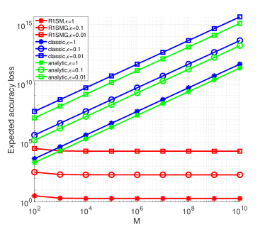
Figure 8: Expected accuracy loss of the R1SMG, classic Gaussian, and analytic Gaussian mechanisms under increasing query size (i.e., $M$) when $\epsilon\in\{0.01,0.1,1\}$ and $\delta=10^{-7}$.

From Figure 8, we observe that, for both classic and analytic Gaussian mechanisms, the expected accuracy loss (i.e., $Tr[\sigma^{2}\mathbf{I}_{M\times M}]$ and $Tr[\sigma_{A}^{2}\mathbf{I}_{M\times M}]$) scales linearly with $M$, which validates our theoretical findings in Section 3. In contrast, as $M$ increases, the expected accuracy loss incurred by the R1SMG mechanism (i.e., $Tr[\bm{\Pi}]=\sigma_{*}$) decreases and converges to $\frac{2(\Delta_{2}f)^{2}}{\epsilon}$. Thus, the R1SMG mechanism not only breaks the curse of full-rank covariance matrices, but also significantly improves the accuracy (utility) of the perturbed $f(\bm{x})$, as it is able to achieve $(\epsilon,\delta)$-DP by using much weaker noise even when the dimension of $f(\bm{x})$ increases.

Appendix C Potential Improvement of the MVG Mechanism

When studying the MVG mechanism, we observe one potential solution to improve its privacy guarantee. In particular, one intermediate step in the proof of the MVG mechanism requires deriving an upper bound for

$$\clubsuit= Tr\Big{[}\bm{\Psi}^{-1}\mathbf{Y}^{T}\bm{\Sigma}^{-1}\Delta+\bm{\Psi}^{-1}\Delta^{T}\bm{\Sigma}^{-1}\mathbf{Y}$$ (20)

$$+\bm{\Psi}^{-1}f(D_{2})^{T}\bm{\Sigma}^{-1}f(D_{2})-\bm{\Psi}^{-1}f(D_{1})^{T}\bm{\Sigma}^{-1}f(D_{1})\Big{]},$$

where $\mathbf{Y}$ stands for the output of the MVG mechanism and $\Delta=f(D_{1})-f(D_{2})$ (see [11] page 244, right column). Due to the negative sign in the fourth term, the authors simply bound its absolute value, i.e., $\big{|}Tr\big{[}\bm{\Psi}^{-1}f(D_{1})^{T}\bm{\Sigma}^{-1}f(D_{1})\big{]}\big{|}$, which results in a very loose upper bound related to the quadratic form in the Frobenius norm of the matrix query result (i.e, $\gamma^{2}$ in Theorem 3), and further compromises the utility.

In fact, the original proof of the MVG mechanism can be improved if we apply the transformation

$$Tr\big{[}\bm{\Psi}^{-1}f(D_{2})^{T}\bm{\Sigma}^{-1}f(D_{2})-\bm{\Psi}^{-1}f(D_{1})^{T}\bm{\Sigma}^{-1}f(D_{1})\big{]}$$

$$= Tr\Big{[}\bm{\Psi}^{-1}\Big{(}f(D_{2})^{T}\bm{\Sigma}^{-1}\big{(}f(D_{2})-f(D_{1})\big{)}+\big{(}f(D_{2})-f(D_{1})\big{)}^{T}\bm{\Sigma}^{-1}f(D_{1})\Big{)}\Big{]},$$

and rewrite $\clubsuit$ as

$$\clubsuit=Tr\Big{[}\bm{\Psi}^{-1}\big{(}\mathbf{Y}-f(D_{2})\big{)}^{T}\bm{\Sigma}^{-1}\Delta+\bm{\Psi}^{-1}\Delta^{T}\bm{\Sigma}^{-1}\big{(}\mathbf{Y}-f(D_{1})\big{)}\Big{]}.$$

Then, we can bound $\clubsuit$ using singular values, and hence the quadratic form in the Frobenius norm of the query result can be completely removed. We do not follow the above steps to further develop an improved version of the MVG mechanism, because the improved version is still a “victim” of the identified curse of full-rank covariance matrices.

References

- [1] Swarm behaviour dataset. https://archive.ics.uci.edu/ml/datasets/Swarm+Behaviour. (Accessed on 02/20/2021).
- [2] Uber pickups in new york city. https://www.kaggle.com/fivethirtyeight/uber-pickups-in-new-york-city. (Accessed on 02/20/2021).
- [3] Martin Abadi, Andy Chu, Ian Goodfellow, H Brendan McMahan, Ilya Mironov, Kunal Talwar, and Li Zhang. Deep learning with differential privacy. In Proceedings of the 2016 ACM SIGSAC conference on computer and communications security, pages 308–318, 2016.
- [4] Mir M Ali. Characterization of the normal distribution among the continuous symmetric spherical class. Journal of the Royal Statistical Society: Series B (Methodological), 42(2):162–164, 1980.
- [5] Borja Balle and Yu-Xiang Wang. Improving the gaussian mechanism for differential privacy: Analytical calibration and optimal denoising. In International Conference on Machine Learning, pages 394–403. PMLR, 2018.
- [6] Amos Beimel, Hai Brenner, Shiva Prasad Kasiviswanathan, and Kobbi Nissim. Bounds on the sample complexity for private learning and private data release. Machine learning, 94:401–437, 2014.
- [7] Tony Cai, Jianqing Fan, and Tiefeng Jiang. Distributions of angles in random packing on spheres. Journal of Machine Learning Research, 14(21):1837–1864, 2013.
- [8] Gabriel Camano-Garcia. Statistics on Stiefel manifolds. Iowa State University, 2006.
- [9] Clément L Canonne, Gautam Kamath, and Thomas Steinke. The discrete gaussian for differential privacy. In H. Larochelle, M. Ranzato, R. Hadsell, M. F. Balcan, and H. Lin, editors, Advances in Neural Information Processing Systems, volume 33, pages 15676–15688. Curran Associates, Inc., 2020.
- [10] George Casella and Roger L Berger. Statistical inference, volume 2. Duxbury Pacific Grove, CA, 2002.
- [11] Thee Chanyaswad, Alex Dytso, H. Vincent Poor, and Prateek Mittal. Mvg mechanism: Differential privacy under matrix-valued query. In Proceedings of the 2018 ACM SIGSAC Conference on Computer and Communications Security, CCS ’18, pages 230–246, New York, NY, USA, 2018. ACM.
- [12] Kamalika Chaudhuri, Anand Sarwate, and Kaushik Sinha. Near-optimal differentially private principal components. Advances in Neural Information Processing Systems, 25:989–997, 2012.
- [13] Yasuko Chikuse. Statistics on special manifolds, volume 174. Springer Science & Business Media, 2012.
- [14] Harald Cramér. Mathematical methods of statistics, volume 43. Princeton university press, 1999.
- [15] Cynthia Dwork, Krishnaram Kenthapadi, Frank McSherry, Ilya Mironov, and Moni Naor. Our data, ourselves: Privacy via distributed noise generation. In Serge Vaudenay, editor, Advances in Cryptology - EUROCRYPT 2006, pages 486–503, Berlin, Heidelberg, 2006. Springer Berlin Heidelberg.
- [16] Cynthia Dwork, Frank McSherry, Kobbi Nissim, and Adam Smith. Calibrating noise to sensitivity in private data analysis. In Theory of Cryptography: Third Theory of Cryptography Conference, TCC 2006, New York, NY, USA, March 4-7, 2006. Proceedings 3, pages 265–284. Springer, 2006.
- [17] Cynthia Dwork and Aaron Roth. The algorithmic foundations of differential privacy. Foundations and Trends® in Theoretical Computer Science, 9(3–4):211–407, 2014.
- [18] Cynthia Dwork and Guy N Rothblum. Concentrated differential privacy. arXiv preprint arXiv:1603.01887, 2016.
- [19] Cynthia Dwork, Guy N Rothblum, and Salil Vadhan. Boosting and differential privacy. In 2010 IEEE 51st Annual Symposium on Foundations of Computer Science, pages 51–60. IEEE, 2010.
- [20] David H Fremlin. Measure theory, volume 4. Torres Fremlin, 2000.
- [21] Arjun K Gupta and Daya K Nagar. Matrix variate distributions. Chapman and Hall/CRC, 2018.
- [22] Moritz Hardt and Kunal Talwar. On the geometry of differential privacy. In Proceedings of the forty-second ACM symposium on Theory of computing, pages 705–714, 2010.
- [23] Michael Hay, Ashwin Machanavajjhala, Gerome Miklau, Yan Chen, and Dan Zhang. Principled evaluation of differentially private algorithms using dpbench. In Proceedings of the 2016 International Conference on Management of Data, pages 139–154. ACM, 2016.
- [24] Kaifeng Jiang, Dongxu Shao, Stéphane Bressan, Thomas Kister, and Kian-Lee Tan. Publishing trajectories with differential privacy guarantees. In Proceedings of the 25th International Conference on Scientific and Statistical Database Management, pages 1–12, 2013.
- [25] Wuxuan Jiang, Cong Xie, and Zhihua Zhang. Wishart mechanism for differentially private principal components analysis. In Proceedings of the AAAI Conference on Artificial Intelligence, volume 30, 2016.
- [26] Norman L Johnson, Samuel Kotz, and Narayanaswamy Balakrishnan. Continuous univariate distributions, volume 2, volume 289. John wiley & sons, 1995.
- [27] Shiva Prasad Kasiviswanathan, Homin K Lee, Kobbi Nissim, Sofya Raskhodnikova, and Adam Smith. What can we learn privately? SIAM Journal on Computing, 40(3):793–826, 2011.
- [28] Chinubhai G Khatri. Some results for the singular normal multivariate regression models. Sankhyā: The Indian Journal of Statistics, Series A, pages 267–280, 1968.
- [29] Alex Krizhevsky, Vinod Nair, and Geoffrey Hinton. The cifar-10 dataset. online: http://www. cs. toronto. edu/kriz/cifar. html, 55(5), 2014.
- [30] Koon-Shing Kwong and Boris Iglewicz. On singular multivariate normal distribution and its applications. Computational statistics and data analysis, 22(3):271–285, 1996.
- [31] Yann LeCun, Léon Bottou, Yoshua Bengio, and Patrick Haffner. Gradient-based learning applied to document recognition. Proceedings of the IEEE, 86(11):2278–2324, 1998.
- [32] Chao Li, Michael Hay, Gerome Miklau, and Yue Wang. A data-and workload-aware algorithm for range queries under differential privacy. Proceedings of the VLDB Endowment, 7(5), 2014.
- [33] Changchang Liu, Supriyo Chakraborty, and Prateek Mittal. Dependence makes you vulnberable: Differential privacy under dependent tuples. In NDSS, volume 16, pages 21–24, 2016.
- [34] Fang Liu. Generalized gaussian mechanism for differential privacy. IEEE Transactions on Knowledge and Data Engineering, 31(4):747–756, 2018.
- [35] Aleksandar Nikolov, Kunal Talwar, and Li Zhang. The geometry of differential privacy: the sparse and approximate cases. In Proceedings of the forty-fifth annual ACM symposium on Theory of computing, pages 351–360, 2013.
- [36] Lu Ou, Zheng Qin, Shaolin Liao, Yuan Hong, and Xiaohua Jia. Releasing correlated trajectories: Towards high utility and optimal differential privacy. IEEE Transactions on Dependable and Secure Computing, 17(5):1109–1123, 2018.
- [37] TensorFlow Privacy. TensorFlow Privacy: MNIST DP-SGD Tutorial. https://github.com/tensorflow/privacy/blob/master/tutorials/mnist_dpsgd_tutorial.py, 2023. Accessed on: 02/24.
- [38] Serge B Provost and AM Mathai. Quadratic forms in random variables: theory and applications. M. Dekker, 1992.
- [39] Wahbeh Qardaji, Weining Yang, and Ninghui Li. Understanding hierarchical methods for differentially private histograms. Proceedings of the VLDB Endowment, 6(14):1954–1965, 2013.
- [40] Calyampudi Radhakrishna Rao and Mathematischer Statistiker. Linear statistical inference and its applications, volume 2. Wiley New York, 1973.
- [41] Horn Roger and R Johnson Charles. Topics in matrix analysis, 1994.
- [42] Kathrin Schacke. On the kronecker product. Master’s thesis, University of Waterloo, 2004.
- [43] Muni Shanker Srivastava and CG Khatri. An introduction to multivariate statistics. 2009.
- [44] Meng Sun and Wee Peng Tay. On the relationship between inference and data privacy in decentralized iot networks. IEEE Transactions on Information Forensics and Security, 15:852–866, 2019.
- [45] TensorFlow. Convolutional Neural Network (CNN). https://www.tensorflow.org/tutorials/images/cnn, 2023. Accessed on: 09/04.
- [46] Peter H Westfall. Kurtosis as peakedness, 1905–2014. rip. The American Statistician, 68(3):191–195, 2014.
- [47] Yonghui Xiao and Li Xiong. Protecting locations with differential privacy under temporal correlations. In Proceedings of the 22nd ACM SIGSAC Conference on Computer and Communications Security, pages 1298–1309, 2015.
- [48] Jungang Yang, Liyao Xiang, Jiahao Yu, Xinbing Wang, Bin Guo, Zhetao Li, and Baochun Li. Matrix gaussian mechanisms for differentially-private learning. IEEE Transactions on Mobile Computing, 2021.
- [49] Jun Zhao, Teng Wang, Tao Bai, Kwok-Yan Lam, Zhiying Xu, Shuyu Shi, Xuebin Ren, Xinyu Yang, Yang Liu, and Han Yu. Reviewing and improving the gaussian mechanism for differential privacy. arXiv preprint arXiv:1911.12060, 2019.