MoviePuzzle: Visual Narrative Reasoning
through Multimodal Order Learning

Abstract

We introduce MoviePuzzle, a novel challenge that targets visual narrative reasoning and holistic movie understanding. Despite the notable progress that has been witnessed in the realm of video understanding, most prior works fail to present tasks and models to address holistic video understanding and the innate visual narrative structures existing in long-form videos. To tackle this quandary, we put forth MoviePuzzle task that amplifies the temporal feature learning and structure learning of video models by reshuffling the shot, frame, and clip layers of movie segments in the presence of video-dialogue information. We start by establishing a carefully refined dataset based on MovieNet [huang2020movienet] by dissecting movies into hierarchical layers and randomly permuting the orders. Besides benchmarking the MoviePuzzle with prior arts on movie understanding, we devise a Hierarchical Contrastive Movie Clustering (HCMC) model that considers the underlying structure and visual semantic orders for movie reordering. Specifically, through a pairwise and contrastive learning approach, we train models to predict the correct order of each layer. This equips them with the knack for deciphering the visual narrative structure of movies and handling the disorder lurking in video data. Experiments show that our approach outperforms existing state-of-the-art methods on the MoviePuzzle benchmark, underscoring its efficacy.

1 Introduction

Humans, even young kids, are capable of quickly perceiving and comprehending different forms of visual media, such as comics, short videos, 3D movies, etc. Without paying attention to details, we connect key visual or auditory information and reason over them in real-time to form a summarized visual narrative [cohn2013visual]. Consider movie frames in Figure 1, one can quickly understand its story as: the male is scamming money over the phone , without counting the accurate number of people in panel E. As such, we can watch and understand long-form videos, movies, and tens of episodes of TV shows. Our approach is predominantly focused on preserving the narrative’s coherence rather than merely reordering shots for non-linear storytelling as seen in conventional montage techniques. It is our belief that any non-linear [frey2021non, park2018non] aspects of the editing should serve the overall narrative, particularly in maintaining the story’s continuity and logic. To further validate the efficacy of our method, we also incorporate extensive human studies to assess the rationality of the generated sequences.

Figure 1: Illustration of movie visual narrative structures. Left: the shuffled movie frames with corresponding dialogues. Right: Recovered visual narrative structure.

As for the computer vision community, video understanding has achieved significant improvements over the past few years, with various benchmarks proposed on fine-grained action predictions [yeung2016end, feichtenhofer2020x3d], Video Question Answering (VideoQA) [fu2021violet, lei2019tvqa, movieqa], and video-grounded dialogue generations [le2020video, le-etal-2022-vgnmn, wang2023vstar], etc. The de facto paradigm is to integrate all extracted dense features of vision and language into a fusion layer w.r.t. their temporal orders [xu2015show, anderson2018bottom]. Despite the inspiring progress of Video-Language models on these tasks, the benchmarks and models commonly neglect two key factors:

Holistic Video Understanding: Fundamentally, most modern literature deviates from the natural setting of comprehending videos in a holistic and abstract manner, i.e., the tasks are treated as multi-frame image understanding problems that target inner-frame and inter-frame modeling. The linearly growing computational cost largely limits the potential of consuming long-form videos like movies and TV shows, which are fulfilled with scene and shot transitions. It is worth noting that some recent works [huang2020movienet] have observed the significance of holistic understanding, while the tasks are still defined as visual recognition and classifications.

Visual Narrative Structures: Beyond the individual visual surface and subtitle lexicons, the ability to perceive and understand a sequence of multimodal images is closely related to the underlying narrative structure, a hierarchical understanding that guides the presentation of events and individual concepts [cohn2013visualbook]. Figure 1 depicts an exemplar illustration: each frame is a brick forming the movie narrative, where irrational swaps may suddenly break integrity.

To address the deficiencies of the prior work and step towards holistic long-form video understanding, we present a new challenge MoviePuzzle that aims at benchmarking the machine’s capabilities on visual narrative reasoning (VNR). In this task, the machine is asked to reorder the sequences of frames to form a plausible narrative; see Figure 1 for an example. We establish a carefully refined dataset based on MovieNet [huang2020movienet]: all frames and corresponding subtitles in a clip are well aligned to form a human-understandable narrative. We further limit the maximum number of the scene and shot transitions within a clip to lower the computational expense of visual perception. The underlying rationale that we choose frame reordering as the main task derives from the preliminary diagnostic studies on visual narrative structures [cohn2013visualbook]. Significantly, various studies have proposed visual reordering as a potential application area [zellers2021merlot, sharma2020deep, epstein2021learning]. However, these primarily concentrate on local temporal consistency and procedural understanding. Contrarily, our approach gives prominence to a comprehensive video understanding and the visual narrative structure. This holistic perspective allows for a more complete and structured interpretation of video content.

Solving MoviePuzzle is intrinsically non-trivial compared with single-frame understanding tasks. We highlight the external requirements on models brought out by VNR: (i) Commonsense Reasoning: the basic knowledge of visual commonsense (underlying rationale of visual activities [zellers2019vcr]) and social commonsense (emotional and social activity understanding [sap2019socialiqa]); (ii) Visual-dialogue Grounding: the ability to integrate information within weakly-aligned dialogues and visual frames; (iii) Visual-dialogue Summarization: the ability to connect individual frames to form a narrative. To probe the machine’s capability for narrative summarization, we add a downstream application as movie synopsis association, where the model is to extract the corresponding synopsis piece with pre-trained VNR models. Besides, we test the generalizability of neural models by splitting the test set into the in-domain test and out-domain test, where the latter are clips selected from unseen movies only with their pre-extracted visual features. We benchmark MoviePuzzle with prior successful models on Movie understanding. To address the structured information existing in the narrative, we further devise a contrastive-learning (CL)-based hierarchical representation for VNR.

To summarize, our contributions are three-fold: (i) We introduce MoviePuzzle, a novel task that aims to facilitate the learning of underlying temporal connections between different plot points in movies by reassembling multimodal video clips; (ii) We construct MoviePuzzle dataset that aligns video clip images and subtitles on a sentence-by-sentence basis. Moreover, we provide annotations for the structural hierarchy of frames, shots, and scenes, all of which are aligned at their boundaries; (iii) We devise a new Hierarchical Contrastive Movie Clustering (HCMC) model and establish a benchmark. Our model outperforms the current baseline models and achieves state-of-the-art results.

2 The MoviePuzzle Dataset

The MoviePuzzle contains a diverse range of data from various modalities and rich annotations on different aspects of movie structures, enabling a comprehensive understanding of movie content. Below we introduce detailed data curation and annotation processes.

2.1 Dataset Curation

Movie

In order to alleviate potential license issues, we use movie sources from an existing large-scale movie dataset pool, MovieNet [huang2020movienet]. Since our task of fine-grained reordering of a multimodal movie hierarchical structure requires frame-level annotations, we carefully filter movies from the original pool by ensuring the existence of frame image, corresponding subtitle file, frame-to-shot boundary, frame-to-scene boundary, and synopsis, resulting in 228 movies with rich tags and a complete semantic structure.

Image & Subtitle

We collect 135,837 movie frames from the metadata. All frames are extracted as RGB images from 240P movies using screenshots, and cropped to remove black borders. In terms of subtitles, we select English subtitle files that are aligned with the movie version. Movies with less than 500 dialogues are discarded. For all subtitles, we discard symbols that are not in Unicode, then remove diacritical marks from foreign vocabulary when transcribing them into English using the 26-letter alphabet, and filter out onomatopoeic subtitles and narrations that represent environmental sounds. Figure 4 shows the wordle of all training utterances. Most lexicons have few relationships with visual objects, challenging vision-dialogue alignment and understanding.

2.2 Refined Data Annotation

Image-utterance pairs

The original MovieNet dataset does not consistently provide corresponding images for each dialogue. Here, we pair each frame image with its corresponding utterance, achieving the finest granularity alignment of images and text on the time sequence. Each dialogue is only matched with the images falling exactly within its corresponding time period, rather than the nearest ones, ensuring the maximum matching of image and text content. In the case of multiple frames falling on a single dialogue, we choose to merge these frames and select the middle frame as the most representative matching image. For most of the original images that do not match with subtitles, we discard them unless they are exceptional examples within a clip for an extended period. Finally, our image-subtitle pairs account for 83.5% of the total frames.

Scene&Shot aligned boundary

Regarding the visual narrative structure of movies as in Figure 1, most clips have two innate hierarchical levels: shots and scenes. A shot is a fixed camera angle capture and typically a short sequence of temporally consecutive frames indicating a few actions. A scene is a sequence of shots that share the same environmental context, which typically depicts an event or a short story. Capturing the hierarchical structure of a movie is vital for movie understanding. Of note, scene segmentation remains an open problem to video understanding [chen2022movies2scenes, rasheed2003scene, rao2020local, chen2021shot]. We leverage annotations from MovieNet [huang2020movienet] to form our labels, including the manually annotated scene boundaries and automatically generated shot boundaries using [shao2018find]. In total, the MoviePuzzle has 15,414 scenes and over 81K semantically rich shots.

Clip aligned boundary

In order to obtain video clips suitable for training, we further segment the 228 movies and ultimately obtain 10,031 movie clips. We use the following two criteria to select appropriate clips as our data: First, each clip should consists of 10 to 20 frames, and the length of the clip is controlled to tell a short plot without the semantic information being too monotonous; Second, the image-text pairs in each clip must be greater than 80%, ensuring the semantics are not too sparse. As shown in Figures 2 and 3, most clips have 1 or 2 scenes (88%) and 5 to 10 separated shots (75.91%), which is in line with the structure of a short plot.

Figure 2: Scenes Distribution

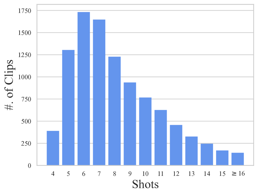
Figure 3: Shots distribution

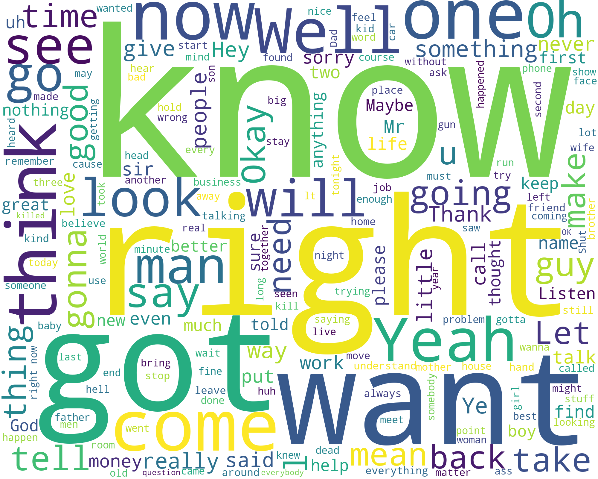
Figure 4: Wordcloud

	all	train	val	in-domain	out-domain
				test	test
#. of Clips	10,031	7,048	589	1,178	1,196

Table 1: Statistics of MoviePuzzle Splits.

2.3 Data Statistics

We divide the entire dataset into four parts: train, val, in-domain test, and out-domain test (Table 1), each accounting for 70%, 6%, 12%, and 12% of the total clips, respectively. The data in val and in-domain test all come from the same set of movies as the train split. We select val and in-domain test by taking equally spaced clips based on the clip numbers from the movie clips covered by the train split. The out-domain test split is entirely taken from different movies as in the train split. This division helps assess the model’s generalization ability.

3 Benchmarking the MoviePuzzle

3.1 Task Formulation

Formally, each clip $C$ within the MoviePuzzle dataset $\mathcal{D}$ can be denoted as a sequence of randomly shuffled but temporally aligned vision-utterance pairs, i.e., $C=\{(v_{1},u_{1}),(v_{2},u_{2}),\cdots,(v_{N_{fm}},u_{N_{fm}})\}\in\mathcal{D}$, with $v_{i}$ and $u_{i}$ index the $i$-th frame and utterance, $N_{fm}$ denotes the number of total frames within a clip. Besides, each frame is labeled with the corresponding shot id $st_{i}$ and scene id $sn_{i}$, identifying the unique shot and scene classes within the movie clip. The goal of the MoviePuzzle challenge is to predict each frame’s temporal index $\{l_{i}\}_{i=1}^{N_{fm}}$. Especially, for a temporally ordered sequence, $idx_{i}=i$ for all frames.

3.1.1 Hierarchical Movie Representations

In this work, we represent an ordered movie clip as a compositional visual narrative structure. From bottom to top, a clip can be represented within frame-level, shot-level, and scene-level; Figure 1 depicts the overall representation.

Frame-Level Representation

We employ $F=\{f_{1},f_{2},\cdots,f_{N_{fm}}\}$ to denote the frame-level representation of a clip $C$, where any $f_{k}\in F$ encompasses all information contained within the $k$-th frame. It includes the visual data $v_{k}$, textual information $u_{k}$, and the corresponding shot identity $st_{k}$ to which the frame belongs.

Shot-Level Representation

For the shot-level representation of a clip, we utilize $G=\{g_{1},g_{2},\cdots,g_{N_{st}}\}$ to represent, where any $g_{j}\in G$ incorporates all information present in the $j$-th shot, and $N_{st}$ signifies the quantity of shots employed in the referred movie clip. This comprises a set of frames $\{f\}_{k=1}^{N_{st}^{j}}$, with ${N_{st}^{j}}$ indicates the frames number in the $j$-th shot. Each represents a frame $f_{k}\in F$ within the shot $g_{j}$, and the associated scene identity $sn_{j}$ to which the shot pertains.

Scene-Level Representation

Similarly, the scene-level representation of a clip is characterized by $H=\{h_{1},h_{2},\cdots,h_{N_{sc}}\}$, with any $h_{i}\in H$ containing all information within the $i$-th scene. This involves a set of shots $\{g\}_{j=1}^{N_{sn}^{i}}$ denoting each shot $g_{j}\in G$ in the scene, where ${N_{sn}^{i}}$ represents the shot number in scene $g_{j}$.

3.1.2 Evaluation Metric

Ordering Score

As defined in Sec. 3.1, the video clip has $N_{fm}$ frames, the ground truth sequence is $\{l_{1},l_{2},\cdots,l_{N_{fm}}\}$, and model ordering prediction sequence is $\{\hat{l}_{1},\hat{l}_{2},\cdots,\hat{l}_{N_{fm}}\}$. We define a match as a $\beta$ length subset of elements that follow their natural order: $i_{1}<i_{2}<\cdots<i_{\beta}$ and $l_{i_{1}}\prec l_{i_{2}}\prec\cdots\prec l_{i_{\beta}}$ and $\hat{l}_{i_{1}}\prec\hat{l}_{i_{2}}\prec\cdots\prec\hat{l}_{i_{\beta}}$, where $\prec$ is a comparator indicating the precedent temporal order. The ordering score is computed as the ratio of the cardinality of the match set:

$$\text{OrderingScore}=\frac{\#\{(i_{k})_{k=1}^{n}|(i_{1}<\cdots<i_{\beta})\wedge(l_{i_{1}}\prec\cdots\prec l_{i_{\beta}})\wedge(\hat{l}_{i_{1}}\prec\cdots\prec\hat{l}_{i_{\beta}})\}}{{\tbinom{N_{fm}}{\beta}}},$$ (1)

where ${\tbinom{N_{fm}}{\beta}}=\frac{N_{fm}!}{\beta!(N_{fm}-\beta)!}$ is the total number of index combinations.

Utilizing this approach, we are capable of procuring evaluation metrics of arbitrary length accuracy, such as when $\beta=\{2,3\}$, which yield pairwise score and triplet score respectively. In this paper, we primarily use the pairwise score because of its significant representativeness.

3.2 Hierarchical Contrastive Movie Clustering

3.2.1 Modeling and Learning

An overview of the Hierarchical Contrastive Movie Clustering (HCMC) model is sketched in Figure 5. At the training stage, we jointly train our model in an efficient end-to-end way. Specifically, the input of our model is the three levels of video-dialogue pairs, including single frame, shot sets, and scene sets. The HCMC model is composed of separate language and image encoders, video-dialogue transformer encoders, pairwise classification heads, and cluster heads. We jointly optimize our model with three-level ordering tasks and two-level clustering tasks .

Multimodal Feature Extractor

Since most popular video-language works [zellers2021merlot, sharma2020deep, epstein2021learning] are not able to obtain the long dependency temporal information, we adopt an end-to-end manner to train our model, aiming to learn a better feature extractor. To mitigate the gap between vision and language, we initialize the vision encoder and language encoder with the parameters of Clip [alec2021clip] vision encoder and language encoder, respectively.

We firstly pass the movie clip $(v_{k},u_{k})$ through Clip vision-language encoder to compute the vision feature token ${\textsc{Clip}}(v_{k})\in\mathbb{R}^{c_{v}\times d}$ and utterance feature tokens ${\textsc{Clip}}(u_{k})\in\mathbb{R}^{c_{u}\times d}$, respectively. $c_{v}$ and $c_{u}$ are token lengths of vision and utterance features, and $d$ is the hidden state length. We aggregate image and text feature tokens by concatenating them across the token length dimension to compute the frame-level representation,

$$F=\{f_{k};f_{k}={{\textsc{Clip}}(v_{k})}\oplus{{\textsc{Clip}}(u_{k})}\}_{k=1}^{N_{fm}}.$$

Here $f_{k}$ indicate the frame $k$’s representation, label $\oplus$ represents the concatenation operator and obtains $f_{k}\in\mathbb{R}^{c\times d}$, where $c=c_{v}+c_{u}$. Regarding the multimodal attributes of shots and scenes, we employ hierarchical cinematic structure features, utilizing the previously acquired lower-level representations of films for depiction:

$$G=\{g^{j};g^{j}=f^{j}_{1}\oplus\cdots\oplus f^{j}_{N_{st}^{j}}\}_{j=1}^{N_{st}},\quad\quad H=\{h^{i};h^{i}=g^{i}_{1}\oplus\cdots\oplus g^{i}_{N_{sn}^{i}}\}_{i=1}^{N_{sn}}.$$

Video-Dialogue Transformer Encoder

After obtaining the embedding of frame and dialogue, we jointly optimize our model with a temporal ordering learning task and a contrastive learning task. For the ordering task, we first concatenate two randomly sampled image-dialogue pairs in the same level and then feed them to the frame-dialogue transformer encoder, after that we use a binary classification head to learn if the input is in the true temporal order.

Notably, to mitigate exposure error, we sample frame-level pairs not only from the same shot. For the clustering task, we sample image-dialogue pairs from different groups as negatives, then optimize the cluster head by attracting the positive and repelling the negative samples.

Learning Objective

We randomly sample an ordered pair of the same layer clips ($\mathcal{P}_{i},\mathcal{P}_{j},\widetilde{\mathcal{Q}}$ ) from the extracted embeddings, where $\mathcal{P}_{i}$ and $\mathcal{P}_{j}$ are two random embeddings belonging to the same level (depending on the layer in which the joint training occurs, the representation can be attributed to the frame, shot, or scene).  and $\widetilde{\mathcal{Q}}=\{\widetilde{\mathcal{Q}}_{1},\widetilde{\mathcal{Q}}_{2},\cdots,\widetilde{\mathcal{Q}}_{n}\}$, where $n$ is the number of negative samples, is the negative data sampled outside the current permutation group. The pair-wise layer representation $(\mathcal{P}_{i},\mathcal{P}_{j})$ is fed into a binary classifier $\phi$, with two classes indicating the forward order ($\mathcal{P}_{i}\succ\mathcal{P}_{j}$) and the backward order ($\mathcal{P}_{i}\prec\mathcal{P}_{j}$) of input pairs. The cross-entropy loss is calculated based on the classifier output. Formally, the objective can be denoted as:

$$\mathcal{L}_{cls}(\mathcal{P}_{i},\mathcal{P}_{j})=CrossEntropy(\phi(\mathcal{P}_{i},\mathcal{P}_{j}),O),$$ (2)

where $O\!\in\!\{0,1\}$ indicates the ground-truth ordering class.

To derive a shot and scene-aware representation, we leverage the Contrastive Learning trick by feeding the output representation to another multi-class classifier $\psi$, where positive and negative data are distinguished based on the contrastive objective:

$$\mathcal{L}_{CL}(\mathcal{P}_{i},\mathcal{P}_{j},\widetilde{\mathcal{Q}})= -\log\frac{\exp(\psi(\mathcal{P}_{i})\cdot\psi(\mathcal{P}_{j}))}{\exp(\psi(\mathcal{P}_{i})\cdot\psi(\mathcal{P}_{j}))+\sum_{k=0}^{n-1}\exp(\psi(\mathcal{P}_{i})\cdot\psi(\widetilde{\mathcal{Q}}_{k}))},$$ (3)

where $\phi(\mathcal{P})\in\mathbb{R}_{+}$ is the representation generated by binary classifier, $\psi(\mathcal{P})\in\mathbb{R}_{+}$ is the representation generated by multi-class classifier.

Taken together, our final objective function is:

$$\mathcal{L}=\mathcal{L}_{cls}+\lambda\mathcal{L}_{CL},$$ (4)

where $\lambda$ is a balancing factor for two objectives.

Figure 5: An overview of frame-level HCMC model.

3.3 Top-down and Bottom-up Inference

We adopt a top-down clustering and bottom-up reordering pipeline approach for the inference.

Reordering Algorithm

For the training data set $X=\{x_{1},\cdots,x_{n}\}$, there exists a confidence score between each pair of instances, represented by the weighted adjacency matrix ${\mathcal{S}}\in\mathbb{R}^{n\times n}$ where ${\mathcal{S}}[i,j]$ denotes the weight that $x_{i}$ is placed directly before $x_{j}$ in the predicted sequence. We use Eqn. 5 to compute the score adjacency matrix:

$${\mathcal{S}}[i,j]\!=\!\frac{\exp{\phi(x_{i},x_{j})[1]-\exp{\phi(x_{i},x_{j})[0]}}}{\exp{\phi(x_{i},x_{j})[1]+\exp{\phi(x_{i},x_{j})[0]}}}.$$ (5)

Our goal is to find a path passing through all $n$ points in the complete graph such that the weight of the path is maximized. We utilize beam search to track the top $bsize$ paths at each iteration to search for local optimal solutions. The algorithm is described in Suppementary.

Top-down and Bottom-up Inference

For each input test data, after going through the multimodel feature extractor, the input feature representation $X=\{x_{1},x_{2},..x_{N_{fm}}\}$ is obtained. We run a top-down and bottom-up inference to obtain the final ordered sequence. We firstly adopt the Top-down strategy for coarse-to-fine clustering scenes and then shots, and then we reorder the different levels of videos from bottom to up. Finally, we obtain the predicted temporal ordering sequence; refer to the Supplementary for the detailed algorithm.

4 Experiments

4.1 Implementation Details

We run all benchmark experiments using a single Nvidia 3090Ti. The model is optimized using AdamW [oord2018representation] with learning rate as $1e-4$ and the following hyperparameters: $\beta_{1}=0.9$, $\beta_{2}=0.999$, $\epsilon=1e-6$. All models are close to convergence with 5 epochs of training. Following [carreira2017quo, feichtenhofer2019slowfast, li2022mvitv2], our input frames are resized to $224\times 224$. Each image is divided into $32\times 32$ patches before going through the Clip encoder. To increase the model’s robustness, we employ a data augmentation strategy that involves using temporally reversed positive samples. We train the learnable embedding layer from scratch, which features two layers of the Bert transformer block with $hidden\_size=512$ and $num\_attention\_heads=8$.

Table 2: Results on movie reordering.  

	in-domain		out-domain
	$\beta=2$	$\beta=3$	$\beta=2$	$\beta=3$
Random	49.66	16.42	49.75	16.59
Bert	53.01	19.44	53.18	19.25
AlBert	54.06	20.30	53.70	19.76
ChatGPT-3.5	49.05	16.52	49.49	16.92
VideoMAE	50.67	18.55	50.83	18.67
Singularity	51.75	18.67	52.33	18.86
HCMC (frame+shot)	55.40	21.58	54.97	21.23
HCMC (frame+scene)	54.93	21.43	54.66	20.67
HCMC (frame+shot+scene)	53.10	19.34	52.84	19.13

Figure 6: Distribution of reordering results w.r.t. frame length.

4.2 Main Results on Movie Reordering

We take different types of prevalent pre-trained temporal models as baselines: language model (Bert [lu2019vilbert], AlBert [li2019visualbert], ChatGPT [openai2023gpt4]), video model (VideoMAE [tong2022videomae]), and video-language model (Singularity [lei2022revealing]). In practice, we follow Bert’s next sentence prediction (NSP) task and AlBert’s sentence-order prediction (SOP) task to predict the temporal relation of the input pair by comparing the probability of binary classification. We take the early fusion strategy to fuse the input dialogue and corresponding frames. The overall results are shown in Table 2 and Figure 6 presents the experimental results across various movie clip lengths. We summarize our key observations as follow:

• ChatGPT limited by lack of specialized training. ChatGPT, excelling within the 3-4 frame ordering, displays limitations under regular lengths. It lacks training for reordered tasks, implying a need for additional training for holistic video understanding.

• Temporal understanding predominantly rooted in dialogue continuity. The robust performance of pure language models like Bert and AlBert suggests that film sequence understanding largely depends on dialogue continuity, underscoring the importance of linguistic context.

• Multimodal models require a greater focus on visual narrative structures. Multimodal models like VideoMAE and Singularity, while showing promise, are yet to fully tackle the task. These models, preoccupied with image and text prediction, underscore the need for a renewed focus on visual narrative structures.

• Multimodal models lack temporal support in image processing methods. Multimodal models’ performance, falling short of pure language models, points to a critical deficiency in current image processing methodologies: the lack of adequate support for temporality.

• Leveraging visual narrative structures is more important in long-form videos. The HCMC model, surpassing other models in multi-frame scenarios with over 5 frames, demonstrates that the effective utilization of visual narrative structures can significantly enhance holistic video understanding. When compared, the HCMC (frame+shot) model performs better than the HCMC (frame+scene) model. This improvement points to the superior granularity provided by the shot structure, particularly when a clip does not contain multiple scenes.

• Three-layer HCMC mitigates cumulative errors better. The superior performance of the three-layer HCMC (frame+shot+scene) compared to its two-layer counterparts suggests that a more layered approach helps in better managing cumulative errors inherent in the pipeline inference method. We demonstrate more details in the ablation studies (Sec. 4.4).

Table 3: Movie Synopsis Association performance. 

	Movie Segment $\rightarrow$ Synopsis				Synopsis $\rightarrow$ Movie Segment
	R@1($\uparrow$)	R@5($\uparrow$)	R@10($\uparrow$)	MedR($\downarrow$)	R@1($\uparrow$)	R@5($\uparrow$)	R@10($\uparrow$)	MedR($\downarrow$)
Random	0.13	0.66	1.32	378.5	0.13	0.66	1.32	378.5
zero-shot	0.26	1.06	2.25	230.5	0.26	1.46	2.65	299.5
zero-shot+recordering	0.40	1.46	3.04	220.0	0.13	1.06	2.78	325.5
Singularity	10.19	30.16	39.95	18.5	6.88	22.35	32.94	24.0
Singularity +recordering	9.92	31.88	43.39	14.0	5.65	20.63	33.47	22.0

4.3 Application on Movie Synopsis Association

We test the holistic understanding capability of movie reordering models on Movie Synopses Associations [xiong2019graph] task with the synopsis metadata from MoviePuzzle. Matching the multimodal semantic segments requires the model to have strong long-form video understanding ability. We boost the best-performance video-language pre-trained model Singularity [lei2022revealing] with temporal ordering objective and hierarchical semantic information. Specifically, we continually train the Singularity with multiple tasks, which add the re-ordering task to the original vision-text contrastive task and matching task. Additionally, we fuse the feature of the scene which is extracted from the pre-trained temporal ordering model to the input for the auxiliary. It is worth noting that different from the original temporal ordering model we drop the subtitle for fairness. We evaluate the performance with standard retrieval metrics: recall at rank N (R@N) and median rank (MedR), which measures the median rank of correct items in the retrieved ranking list. As shown in Table 3, we observe that our method boosts the performance of the video-to-text retrieval task more significantly than the text-to-video retrieval task. The reason is that our method is helpful in building a long-form video representation while doing no good to the vision-language fusion mechanism. Furthermore, we apply the zero-shot embedding matching method. In practice, we take the clip feature as a baseline and augment it with scene features extracted by our temporal ordering model. Line 2-3 shows zero-shot results similar to Singularity.

4.4 Ablation Studies

	in-domain		out-domain
	$\beta=2$	$\beta=3$	$\beta=2$	$\beta=3$
HCMC (frame+shot)	55.40	21.58	54.97	21.23
w/o shot	54.21	20.41	54.29	20.19
w/o CL	52.63	18.79	52.74	18.05
w/o text	50.05	17.53	49.86	17.40
w/o vision	51.69	18.36	51.87	18.67

Table 4: Ablated HCMC models. 

Table 4 shows the ablation experiments of different components in the HCMC model. The accuracy of the experiments decreases when any layer shown in the table is removed. Among them, removing the textual information in the clip has the most significant impact on the model, followed by the image information. It can be seen that the MoviePuzzle task relies heavily on multimodal information, which is consistent with our intuition. When contrastive learning or the shot layer is removed from the model, the accuracy of the model also decreases.

		in-domain			out-domain
		IoU	$\beta=2$	$\beta=3$	IoU	$\beta=2$	$\beta=3$
Euclidean	shot	37.56	54.93	21.41	35.74	54.98	21.33
	frame	-	55.40	21.58	-	54.97	21.23
Cosine	shot	36.9	54.42	20.49	36.70	55.17	21.31
	frame	-	54.77	21.15	-	55.10	21.28
Soft_DTW	shot	16.94	52.71	18.04	16.85	53.49	19.83
	frame	-	53.24	19.94	-	54.70	20.94

Table 5: Accumulation error analysis.

Accumulative Error

As mentioned before, our three-tier fine-grained model with both shot and scene clustering modeling obtains poor performance. We believe the accumulative error from the clustering layer and re-order layer causes this. Thus we quantitatively analyze the intermedia result of different stages. Table 5 shows the inter-media score of the shot clustering and frame ordering among different distance functions. We calculate the Intersection-over-Union (IoU) score of the shot clustering for reference. Specifically, we match the cluster centers with the mean of the ground truth cluster through cosine similarity. The results demonstrate the shot clustering score is positively correlated with the shot ordering score. However, the drop ordering score is more mitigated than the clustering score, i.e., soft_DTW [Cuturi2017SoftDTWAD]. This is because the soft_DTW method results in more empty clusters than others.

4.5 Human Study

As discussed in Sec. 3.1.2, the numerical comparison between the predicted order and ground truth may not always be the best metric. To verify our model’s inherent understanding of movie logic, we recruited 10 well-educated human testers with proficient English comprehension skills to compare the logical coherence of generated clip sequences. Specifically, we select 20 sets of test data from both in-domain and out-domain sources and fed them into the best-performing baseline model AlBert, our HCMC model and ground truth for prediction. Figure 7 showcases a random example. It is notable that even in sections where the AlBert model completely misplaces frames, our model can still ensure accuracy within the same shot. We then present the predicted sequences to testers, who are asked to choose the more reasonable sequence without knowing which model generated it. The orders of the two predicted sequences are randomly shuffled for each comparison test. The comparison results in Table 6 demonstrate that the sequences generated by our approach are more in line with human preferences with AlBert.

	all	in-domain	out-domain
HCMC (Ours) v.s. AlBert	0.55	0.54	0.56
HCMC (Ours) v.s. Ground Truth	0.26	0.23	0.30

Table 6: Human preferences.

In comparison to the ground truth, there is approximately a 26.5% likelihood for testers to select the images generated by our model. This is because there are often multiple plausible scenarios for rational frame reordering in films, as exemplified in the provided image Figure 8.

Figure 7: Qualitative comparisons on reordering performance between AlBert and HCMC (Ours). The red rectangles highlight misplaced frames, while the yellow ones denote misplaced shots (with correct inner frame orders). Our models excel in grouping together frames that share similar shot information, thereby forming a more plausible visual narrative. 

Figure 8: Qualitative comparisons between Ground Truth and HCMC (Ours). In this context, the temporal sequence of Elizabeth stepping forward to receive the gift and the male host delivering a speech can be considered interchangeable. The HCMC model demonstrates a rational interpretation of the narrative.

5 Conclusion

This work presents the novel task MoviePuzzle, aiming to facilitate learning latent associations between movie plot points via recombining multimodal clips. We curate a new dataset aligning video clip images and text frame-by-frame, sentence-by-sentence, supplemented with annotations for the structural hierarchy of frames, shots, and scenes. Moreover, we devise a Hierarchical Contrastive Movie Clustering (HCMC) model, establishing a task benchmark.

Despite the improved performance presented in sufficient experiments, there still remains a huge challenge toward better ordering performance, especially when it comes to long sequences of shuffled frames. One major limitation of the current framework is the lack of global temporal consistency modeling due to the pressure of computational cost. Another limitation lies in the assumption that frames sharing the same shot or scene information shall be grouped together, whereas in a realistic setting, shots may switch back and forth according to the video editing arts. Nonetheless, by presenting MoviePuzzle and preliminary experiments, we aspire to illuminate future avenues for video comprehension research.

We provide supplementary materials as follows:

• Appendix A is the related work.

• In Appendix B, we described the steps we took to collect and preprocess our dataset.

• Appendix C presented the experimental hyperparameters and implementation details of our main experiment.

• In section Appendix D, we investigated the impact of clip length on experimental results.

• Appendix E provided a detailed description of our inference algorithm.

• Appendix F introduced alternative model designs and presented experimental findings.

• In Appendix G we discussed potential ethical risks associated with our paper.

• Appendix H displayed some qualitative result images.

Appendix A Related Work

Joint representation of images and text

Joint image-text representations [bengio2013representation] benefit many language-and-vision tasks by fusion of the modalities. A family of “VisualBERT” models [tan2019lxmert, chenuniter, alberti2019fusion, li2019visualbert, lu2019vilbert, yu2021ernie, gan2020large] have been proposed a common method which uses a supervised object detector image encoder backbone and pre-train on image-caption pairs. Cross-modal representations are learned through masked language modeling objective [kenton2019bert] Another family of vision-language models is based on contrastive learning [alayrac2020self, bain2021frozen, li2021align, alec2021clip, yao2021filip], which have a solid ability to extract features on static image-caption pairs. Some other models like Flamingo [alayrac2022flamingo] and Blip-v2 [li2023blip] use a lightweight transformer to bridge the modality gap between a frozen image encoder and a frozen large language model (LLM). Our method differs from these approaches as these approaches use an explanate image-text representation which keeps unchanged when learning different semantic structures.

Video-language understanding

As an application of artificial intelligence in the multi-media field, video-language understanding has drawn great attention in the research community, such as video story telling [huang2016visual], video moment retrieval [chen2020fine], image caption [hou2020joint, yang2019auto], visual question answering [li2019relation], and action recognition [wang2018non]. Prior arts before the large-scale pre-training era [lei2018tvqa, lei2019tvqa, le2020hierarchical] leverage offline extracted video features [kay2017kinetics], after that, video-language pre-trained models [li2020hero, zhu2020actbert] have shown promising results. Aligned with the success of transformer-based [vaswani2017attention] language pre-training models [liu2019roberta, yang2019xlnet], image-text pre-training [li2019visualbert, he2022masked] and video-text pre-training [kim2021self, fu2023empirical-mvm] usually use masked visual modeling and have shown promising results on short videos clips. These models underutilized temporal information in long videos [zellers2021merlot, huang2020movienet].

Movie Benchmarks

A couple of research works have addressed the importance of understanding long-form videos, especially movies [lsmdc, ava, laptev2008movie-act, Bha2014cls]. For example, MovieQA [movieqa] is extracted from 408 movies with 15K questions. This dataset is designed by using QA to evaluate story understanding. MovieGraph [moviegraphs] is a small dataset with graph-based annotation of social relationships depicted in clips edited from 51 movies. With the relation graph of character, interaction, and attributions, MovieGraph can offer a hierarchical structure of movie understanding. MovieNet [huang2020movienet] is a comprehensive movie dataset with diverse annotations, supporting in-depth movie understanding. Covering 1,100 movies, not all are adequately annotated or aligned. We meticulously filter and organize this dataset to derive well-labeled, aligned subsets within a movie hierarchy.

Appendix B Data Collection Information

B.1 Selecting Movie

We employ the following top-level criteria for choosing the movie source and its associated transcripts from MovieNet [huang2020movienet] for MoviePuzzle:

1. The movies should have color images, and the quality of the picture should not be too dark or blurry.

2. The movies should have English subtitles, as some movies in the original MovieNet dataset either have missing subtitles or have subtitles in languages other than English.

3. The movies should have synopsis summaries to assist in downstream Movie Synopsis Association tasks. However, it should be noted that only a subset of movies in the original MovieNet dataset have synopsis labels.

4. The movies should have a list of actors. We plan to add character labels to the dialogue in future work.

5. The movies should have defined boundaries for shots and scenes.

B.2 Aligning Subtitle

We match each frame image with its corresponding subtitle using the following steps:

1. Firstly, we remove most voiceovers and background sounds from the subtitles and replace foreign words with English letters with tones.

2. Secondly, each dialogue is only paired with images that fall exactly within its corresponding time period, rather than the closest ones.

3. Finally, in the case of multiple frames falling on a single dialogue, we merge these frames and select the middle frame as the most representative matching image.

B.3 Cutting into Clips

We segment the movie into clips based on the following criteria, where the textual subtitles are aligned frame by frame:

1. The length of each clip is restricted to 10-20 frames.

2. The frames containing subtitles in each clip must account for more than 80% of all.

3. A greedy algorithm is utilized to match the movie for as long as possible.

After obtaining a total of 10,031 movie clips, we split the data into training, validation, in-domain test, and out-of-domain test sets in the proportions of 70%, 6%, 12%, and 12%, respectively. The dataset will be publicly released at a later date.

Appendix C Additional Implementation Details

The hyper-parameters we use are shown in Table 7 below. Our Clip [alec2021clip] (clip-vit-base-32) and Bert [kenton2019bert] (bert-base-uncased) parts code uses from HuggingFace.

Hyperparam	HCMC
Number of Transformer Layers	2
Hidden Size	512
Attention Heads	8
Attention Heads Size	64
Learning Rate	1e-4
Batch Size	8
Max Cluster Steps	1000
Cluster Distance	Euclidean
Epoch	5
AdamW $\epsilon$	1e-6
AdamW $\beta_{1}$	0.9
AdamW $\beta_{2}$	0.999
Weight Decay	0.01
Patch Size	32

Table 7: Hyperparameters for HCMC.

Appendix D More Numerical Results

We conducted an experiment to compare the impact of different sequence lengths on the performance of our model, as illustrated in the Figure 9 below. As the sequence length increases, the overall accuracy of the model demonstrates a declining trend, particularly within the range of 13 to 17 where the decline is more pronounced. These results suggest that the model’s ability to process sequences diminishes as the length of the sequence increases.

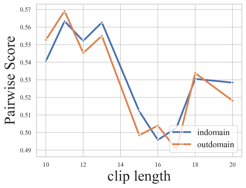
(a) Pairwise Score.

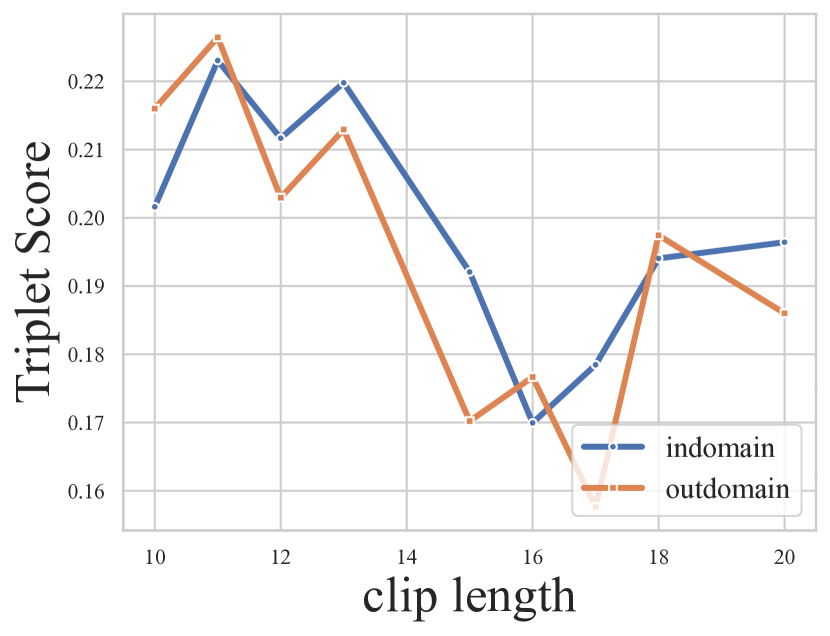
(b) Triplet Score.

Figure 9: Ablated results on clip length.

We also investigate the impact of the number of hierarchical structures on experimental results through ablation experiments. Figure 10(b) shows the results of running the frame+shot HCMC model with the lengths of frames within shots controlled at 1, 2, and 3 in the entire video clip. For the in-domain test dataset, the accuracy slightly decreases when the length increases from 1 to 2, but then rapidly increases to its maximum value when the length increases to 3. For the out-domain test set, the model’s performance gradually improves with the increasing complexity of the data. The results presented in Figure 10(a) depict the outcome of utilizing the frame+scene HCMC model to manipulate the lengths of frames within shots at 1, 2, and 3 in the entire video clip. For both the in-domain and out-domain test datasets, the accuracy increases with the increasing length of frames in scenes. From the ablation experiments, it can be concluded that, in general, data with hierarchical structures can be helpful for the model to understand video clips.

(a) Shot Length.

(b) Scene Length.

Figure 10: Ablated results on video sampling lengths.

Appendix E Inference Algorithm

We adopt a top-down clustering and bottom-up pipeline approach for the reordering inference. Specifically, we adopt the Top-down strategy for coarse-to-fine clustering scenes and then shots, and then we reorder the different levels of videos from bottom to up. Suppose $X=\{x_{1},x_{2},\cdots,x_{N_{fm}}\}$ is a list of shuffled video frames clip, with ground truth index set $\{l_{1},l_{2},\cdots,l_{n}\}$. We complete the inference in five steps as follows and Algorithm 1:

Frame cluster to scene

We use the output of the scene-level cluster head of HCMC as the feature for k-means clustering. We can obtain the current scene layer clustering groups as

$$\hat{X}^{1}=\{g_{k};g_{k}=\{x^{k}_{1},\cdots,x^{k}_{N^{k}_{sn}}\}\}_{k=1}^{N_{sn}},$$

where each group $h_{k}$ represents the index of the elements in the same scene.

Frame cluster to shot

After clustering the scene groups as $H$, we use the output of the shot-level cluster head of HCMC as the feature for k-means clustering on shot. At this point, we obtain the grouping of the shot-level clustering as

$$\hat{X}^{2}=\{g_{k};g_{k}=\{f^{k}_{i},f^{k}_{i}=\{x^{k,i}_{j}\}_{j=1}^{N_{st}^{k,i}}\}_{i=1}^{N^{k}_{sn}}\}_{k=1}^{N_{sn}}.$$

Frame-level reordering

After grouping by shot, we can use the frame-level classification head of HCMC to sort the frames in each shot. We can obtain the output vector $p$ between any two frames using a binary classifier, and use the difference in softmax to represent the confidence of the order representation. In this way, we can obtain a weight value between any two frames, and we can obtain an adjacency list. We use beam search to search for the maximum weight arrangement, representing that we have sorted the order of all scenes on a clip using binary classification. At this point, the order becomes

$$\hat{X}^{3}=\{g_{k};g_{k}=\{f^{k}_{i},f^{k}_{i}=\{\hat{x}^{k,i}_{j}\}_{j=1}^{N_{st}^{k,i}}\}_{i=1}^{N^{k}_{sn}}\}_{k=1}^{N_{sn}}.$$

Shot-level reordering

After reordering frames for each shot, we sort the shots in each scene. Firstly, we use the concatenated features of each frame in the shot to represent the current shot feature. Then we use the shot-level classification head of HCMC to obtain an adjacency list representing the order confidence. We then use the same beam search method to find the ordering with the maximum total confidence. At this point, the order becomes

$$\hat{X}^{4}=\{g_{k};g_{k}=\{\hat{f}^{k}_{i},\hat{f}^{k}_{i}=\{\hat{x}^{k,i}_{j}\}_{j=1}^{N_{st}^{k,i}}\}_{i=1}^{N^{k}_{sn}}\}_{k=1}^{N_{sn}}.$$

Scene-level reordering

Finally, we sort the scenes by pairing the features of these scenes, using the scene-level classification head of HCMC model to obtain an adjacency list representing the order confidence, and then using the same beam search method to find the ordering with the maximum total confidence. At this point, the scene layer has been ordered as

$$\hat{X}^{5}=\{\hat{g}_{k};\hat{g}_{k}=\{\hat{x}^{k}_{1},\cdots,\hat{x}^{k}_{N^{k}_{sn}}\}\}_{k=1}^{N_{sn}},$$

Expanding it into a one-dimensional list $\hat{X}=\{\hat{x}_{1},\cdots,\hat{x}_{N_{fm}}\}$ and gaining its index list represents the order of the prediction as $\{\hat{l}_{1},\hat{l}_{2},\cdots,\hat{l}_{n}\}$.

1

Input: temporally shuffled sequence $X$, classifier embedding layer $\phi$, clusterer embedding layer $\psi$, scene count $N_{sn}$, shot count ${N_{st}}$, beam search width $bsize$

Output: temporally ordered sequence $Y$

/* 1. scene clustering */

2 $X\leftarrow KmeansClustering(\psi(X),N_{sn})$

/* 2. shot clustering */

3 $tmp\leftarrow$ empty set

4 for $scene$ in $X$ do

5       $tmp$.add($KmeansClustering(\psi(scene),{N_{st}^{scene}}$)

6      

7$X\leftarrow tmp$

/* 3. frame reordering */

8 for $scene$ in $X$ do

9       for $shot$ in $scene$ do

10             ${\mathcal{S}}\leftarrow$ substitute $shot$ into weighted adjacency matrix

11             $path\leftarrow BeamSearch({\mathcal{S}},bsize)$

12             Sort the $shot$ in $X$ based on the sequence $path$

13            

14      

/* 4. shot reordering */

15 for $scene$ in $X$ do

16       ${\mathcal{S}}\leftarrow$ substitute $scene$ into weighted adjacency matrix

17       $path\leftarrow BeamSearch({\mathcal{S}},bsize)$

18       Sort the $scene$ in $X$ based on the sequence $path$.

19      

/* 5. scene reordering */

20 ${\mathcal{S}}\leftarrow$ substitute $X$ into weighted adjacency matrix

21 $path\leftarrow BeamSearch({\mathcal{S}},bsize)$

22 Sort the $X$ based on the sequence $path$.

23 return $X$

Algorithm 1 Top-down and Bottom-up Inference

E.1 Kmeans Clustering Algorithm

Suppose we have a training set $X=\{x_{1},\cdots,x_{n}\}$, and want to group the data into a few cohesive clusters. Here, we are given feature vectors for each data point $x_{i}$ with no labels as an unsupervised learning problem. Our goal is to predict $m$ centroids and a label $z_{i}$ for each data point. Then cluster sequence $x$ into $m$ groups based on its corresponding $z_{i}$ to obtain a new sequence $Y=\{y_{1},\cdots,y_{m}\}$, where $Y$ is a partition of $X$. The kmeans clustering algorithm is as Algorithm 2:

Input: training set ${X}$, number of clusters $m$, max number of steps $K$

Output: The clustered sequence $Y$

1 Initialize cluster centroids $\mu_{1},\cdots,\mu_{m}\!\in\!\mathbb{R}^{m}$ randomly

2 foreach $i$ do

3       $z_{i}\leftarrow{\rm arg}\mathop{{\rm min}}\limits_{j}\lVert x_{i}-\mu_{j}\lVert^{2}$

4foreach $j$ do

5       $\displaystyle\mu_{j}\leftarrow\frac{\sum_{i=1}^{n}1\{z_{i}=j\}x_{i}}{\sum_{i=1}^{n}1\{z_{i}=j\}}$

6Repeat step 2-7 until convergence or reaching max cluster steps

7 $Y\!\leftarrow X^{\prime}s$ partition that for all $x_{i}\in y_{j}$ have same $z_{i}$

8 return $Y$

Algorithm 2 KmeansClustering

E.2 Beam Search Algorithm

For the training data set $X=\{x_{1},\cdots,x_{n}\}$, there exists a confidence score between each pair of instances, represented by the adjacency matrix ${\mathcal{S}}$ where ${\mathcal{S}}$ size is $n\times n$ and ${\mathcal{S}}[i,j]$ denotes the weight that $x_{i}$ is placed directly before $x_{j}$ in predict sequence. Our goal is to find a path passing through all $n$ points in the complete graph such that the weight of the path is maximized. We utilize beam search to keep track of the top $bsize$ paths at each iteration to search for local optimal solutions. The algorithm is described in Algorithm 3.

Input: ${\mathcal{S}}$(weighted adjacency matrix), $bsize$

Output: $path$

1 ${bestlist}\leftarrow empty$

2 $n\leftarrow$ length of ${\mathcal{S}}$

3 for $begin$ in $n$ do

4       ${beamlist}\leftarrow\{begin\}$

5       $len\leftarrow 1$

6       while $len<n$ do

7             ${newlist}\leftarrow empty$

8             for $beamPath$ in ${beamlist}$ do

9                   ${newlist}$.add({$beamPath+i$, for all node $i$ not in $beamPath$})

10                   ${newlist}\leftarrow$ top $bsize$ score path in ${newlist}$

11                  

12            ${beamlist}\leftarrow{newlist}$

13             $len\leftarrow len+1$

14            

15      ${bestlist}$.add(max score path in ${beamlist}$)

16      

17$path\leftarrow$ max score path in ${bestlist}$

18 return $path$

Algorithm 3 BeamSearch

Appendix F Alternative Design

We have experimented with model structures trained separately at the frame, shot, and scene levels, in addition to the joint end-to-end training structure introduced in the main body of the paper. We also want to try layered experiments in addition to see how the combined training model can help.

In essence, we trained three parallel independent models, each having a similar structure. For the Video-Dialogue Encoder layer, we have tried using both a simple MLP structure and a simple transformer block. The result shows that these single-layer training models achieved satisfactory results in their respective layers (as shown in rows 1-3 of  Tables 8 and 9). However, when employing the trained single-layer models for multi-layer inference (as shown in row 4-6 of  Tables 8 and 9), the lack of inter-layer connections led to a rapid decrease in model performance.

In addition to the aforementioned experiments, we conducted an ablation study on the hyperparameter $\lambda$, as denoted in the loss function of the main manuscript. By performing a grid search in the range between 0 and 1, as shown in Table 10, we observed the optimal performance when lambda is set to 0.75. It is noteworthy that in the penultimate row of the table, even when introducing the contrastive learning (CL) loss term with a relatively small weight of 0.25, we still achieved a significant improvement. This evidence highlights the effectiveness of the CL approach in the training process of the HCMC model.

	in-domain		out-domain
	pair.	triplet.	pair.	triplet.
frame	59.75	22.67	59.98	23.06
shot	58.40	21.58	58.97	21.23
scene	58.93	20.43	58.66	20.67
frame+shot	51.21	17.95	51.54	18.01
frame+scene	50.94	18.14	51.49	17.79
frame+shot+scene	50.10	16.54	50.54	16.68

Table 8: Results on MLP training separately.

	in-domain		out-domain
	pair.	triplet.	pair.	triplet.
frame	61.12	23.01	63.73	23.93
shot	59.43	22.44	59.54	22.25
scene	59.52	21.30	60.12	22.06
frame+shot	51.99	18.12	52.28	18.67
frame+scene	51.54	17.55	51.83	18.32
frame+shot+scene	50.65	17.06	51.52	17.11

Table 9: Results on Transformer training separately.

$\lambda$	in-domain		out-domain
	pair.	triplet.	pair.	triplet.
1.00	55.40	21.58	54.97	21.23
0.75	55.93	22.20	55.21	21.80
0.50	54.28	21.33	54.68	21.02
0.25	53.98	19.82	53.31	20.47
0.00	52.63	18.79	52.74	18.06

Table 10: Ablation study on CL loss weight $\lambda$.

Appendix G Ethics Concern

Were any ethical review processes conducted (e.g., by an institutional review board)? No official processes were done, as our research is not on human subjects, but we had significant internal deliberation when choosing the movies.

Does the dataset contain data that might be considered confidential? No, our data comes from existing public movie data sets.

Does the dataset contain data that, if viewed directly, might be offensive, insulting, threatening, or might otherwise cause anxiety? If so, please describe why. Yet – few of these videos exist; There may be horror films and things like profanity, but all the films have been censored for public screening.

Does the dataset identify subpopulations (e.g., by age or gender)? Not explicitly.

Is it possible to identify individuals (i.e., one or more natural persons) directly or indirectly (i.e., in combination with other data) from the dataset? Yes, our data include celebrities or other film actors. All of the videos we use are publicly available datasets.

Appendix H Qualitative Image

Refer to Figures 11, 12, 13, 14, 15 and 16 for qualitative comparisons. Figures 11, 12 and 13 come from in domain test data set and Figures 14, 15 and 16 come from out domain test dataset. From these examples, it can be observed that our method is able to arrange the same shots closer together within a movie clip compared to the baseline, resulting in an overall better reordering performance.

(a) Ground Truth

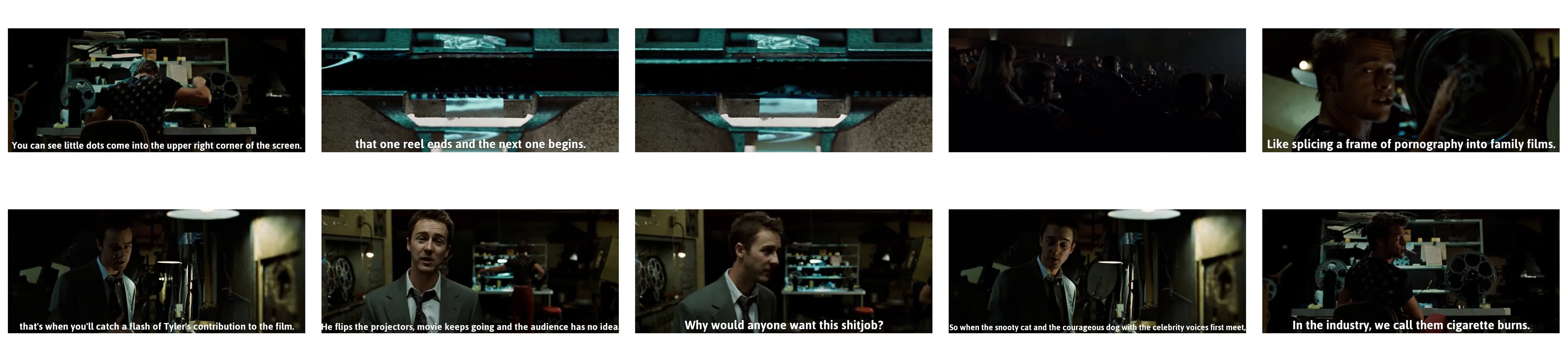
(b) HCMC

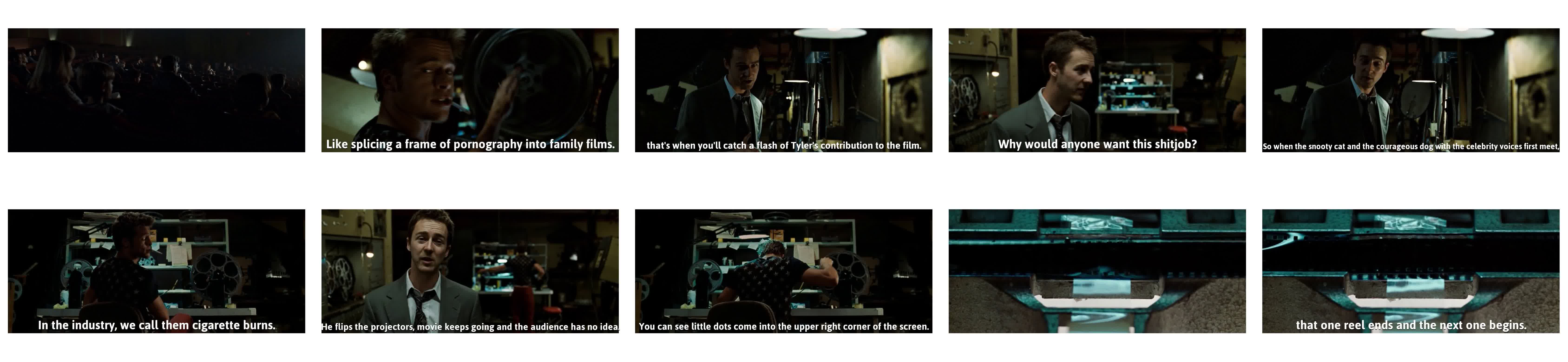
(c) Baseline

Figure 11: Movie: Fight Club. Synopsis: After one meeting, he confronts her. She argues that she’s doing exactly what he does and quips that the groups are ’cheaper than a movie and there’s free coffee. Instead of ratting each other out, they agree to split up the week and exchange numbers. Despite his efforts, the narrator’s insomnia continues. On a flight back from one of his business trips, the narrator meets Tyler Durden. Tyler offers a unique perspective on emergency procedure manuals in the plane and they strike up a casual conversation. Tyler is a soap salesman, if he’s not working nights as a projectionist and slipping bits of porn between reels. The narrator arrives at the baggage claim to discover that his suitcase has been confiscated, most likely due to a mysterious vibration, before he taxis home. However, home, a fifteenth story condominium, has been blasted into the night by what was theorized to be a faulty gas line ignited by a spark on the refrigerator. Having nowhere to go, the narrator finds a business card for Tyler and calls him up. They meet in a parking lot behind a bar where Tyler invites the narrator to ask to come live with him…on one condition: that the narrator hit Tyler as hard as he can. The narrator, though puzzled, complies and they engage in a fist fight before sharing a couple of drinks. The experience is surprisingly euphoric.

(a) Ground Truth

(b) HCMC

(c) Baseline

Figure 12: Movie: Bruce Almighty. Synopsis: Racing back to the station, Bruce gets caught in traffic and vents his frustration about the fact that his life is in a go-nowhere rut. Arriving late to an important meeting, fellow staffers–including nemesis Evan Baxter (Steve Carrell)–needle Bruce mercilessly about his clownish coverage at the bakery, further exacerbating his bitterness about being stalled on his career path. In the exchange with Evan, we see that Bruce has a lively, but dark, sense of humor and won’t take anything lying down. After the meeting, Bruce begs his boss, Jack Baylor (Philip Baker Hall), to consider him for the open anchor position.

(a) Ground Truth

(b) HCMC

(c) Baseline

Figure 13: Movie: Wanted. Synopsis: One night at a pharmacy, Gibson meets a mysterious woman who tells him his father was an elite assassin who had been killed the day before. Gibson replies that his father abandoned him a week after his birth. At that moment, Cross appears, gun in hand. The woman opens fire on Cross. Gibson and the woman escape from the resulting shoot-out and have a wild car chase in the streets of Chicago. The woman brings Gibson to the headquarters of The Fraternity, a thousand-year-old secret society of assassins. The group’s leader, Sloan (Morgan Freeman), formally introduces Gibson to Fox (Angelina Jolie), the woman from the night before, and invites him to follow in his father’s footsteps as an assassin. Sloan tests Gibson by making him shoot the wings off a fly. When Gibson refuses, a gun is put to his head, triggering a panic attack. Gibson somehow manages to shoot the wings off several flies. Sloan says that he was able to do that because his heart beats 400 times a second when he’s stressed. When Sloan asks him whether he want to know how to control it, he runs away in fear. Gibson wakes up the next day hoping everything was a dream, but discovers his father’s gun (which he stashes in the toilet tank), and that he has $3.6 million in his bank account. At work, Gibson tells off his boss, bashes his duplicitous friend with a computer keyboard, and storms out. Gibson then sees pictures of himself and Fox on the front page of several newspapers as wanted fugitives for the pharmacy shooting. Then he notices Fox, who has been waiting outside, and she gives him a ride back to the Fraternity headquarters - an unassuming textile mill.

(a) Ground Truth

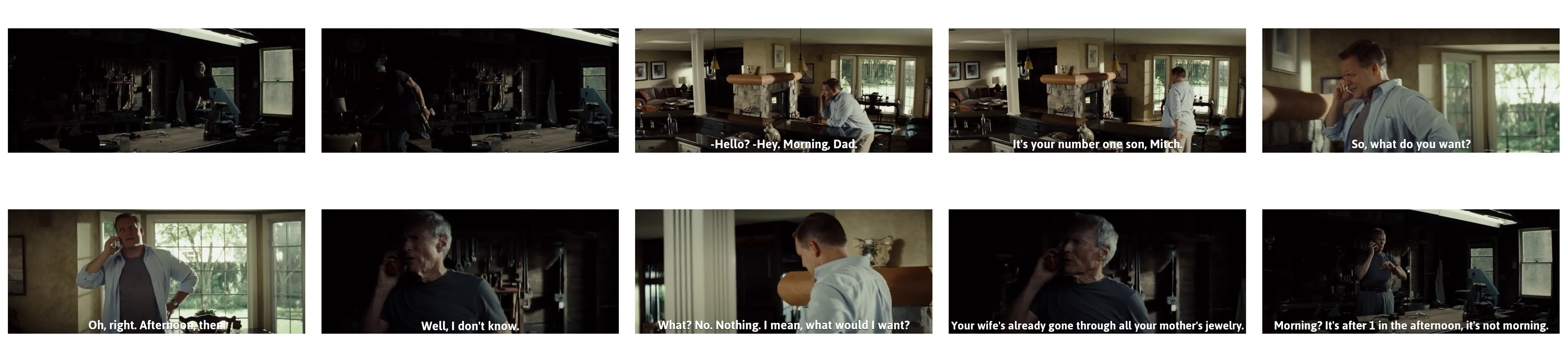
(b) HCMC

(c) Baseline

Figure 14: Movie: Gran Torino. Synopsis: Mitch and his wife, Karen (Geraldine Hughes) go to visit Walt on his birthday, bringing him a cake and a few gifts meant to make certain menial tasks easier. Presentation, and explanation, of these gifts quickly turn into a shamelessly brazen pitch to get Walt to move into a senior’s retirement home. Knowing that Mitch and Karen just want to get their hands on his house, Walt growls in anger and throws them out; gifts, cake and all. Mitch and Karen cannot understand Walt’s reaction.

(a) Ground Truth

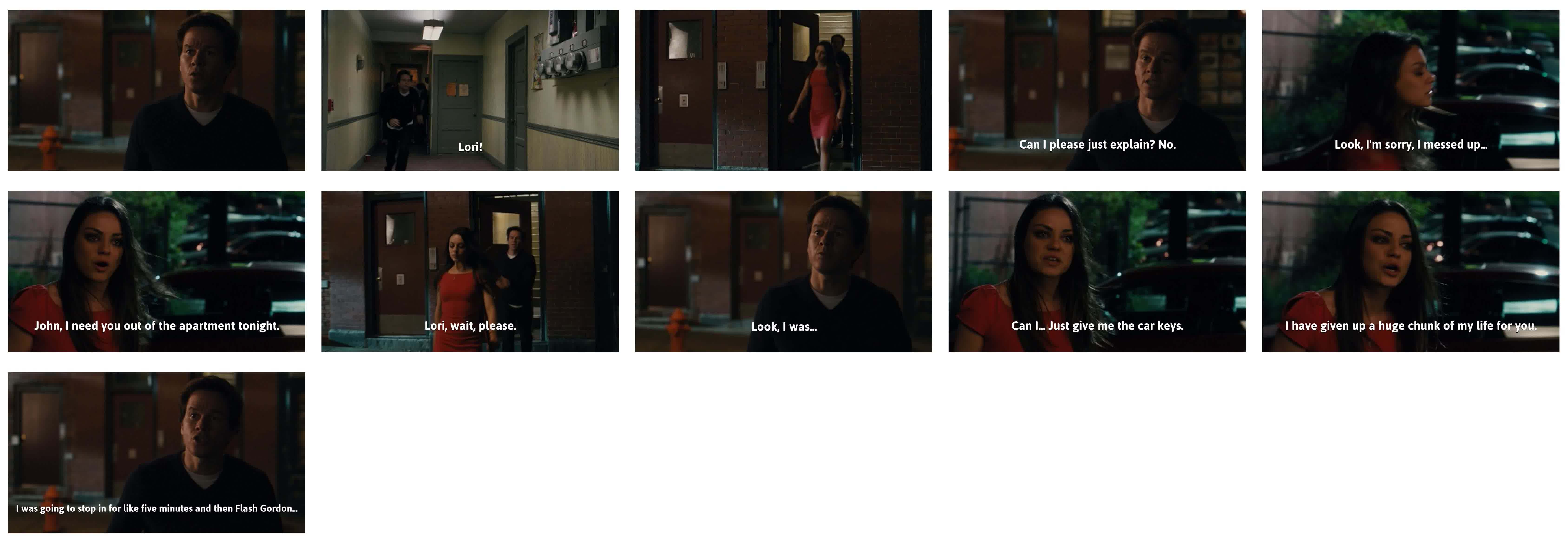
(b) HCMC

(c) Baseline

Figure 15: Movie: Ted. Synopsis: John finds Ted his own apartment and a job at a grocery store, where his grossly irresponsible behavior on the job manages to both get him promoted and acquainted with the superficial co-worker Tami-Lynn (Jessica Barth), who gets easily irritated by Lori who is shocked at her anger. Regardless, Ted and John still spend most of their time together, which frustrates Lori when she discovers John has been skipping work to do so while using her for his excuses. Meanwhile, a crazed loner named Donny (Giovanni Ribisi), who idolized Ted as a child, shows interest in possessing him for his brutishly destructive son, Robert (Aedin Mincks). Things start to come to a head when Lori and John are invited to a party put on by Lori’s lecherous manager, Rex (Joel McHale), and Ted lures John away to a wild party at his apartment with the offer to meet Sam J. Jones (playing himself), the star of their favorite movie, Flash Gordon. Although John arrives with the intention of spending only a few minutes, he gets caught up in the occasion which gets completely out of control, with Sam J. Jones persuading John and Ted to snort cocaine and Ted singing karaoke and eventually getting beaten-up by a duck. Eventually, Lori discovers John there and breaks up with him in a rage. At that, John blames Ted for ruining his life and tells him to stay away.

(a) Ground Truth

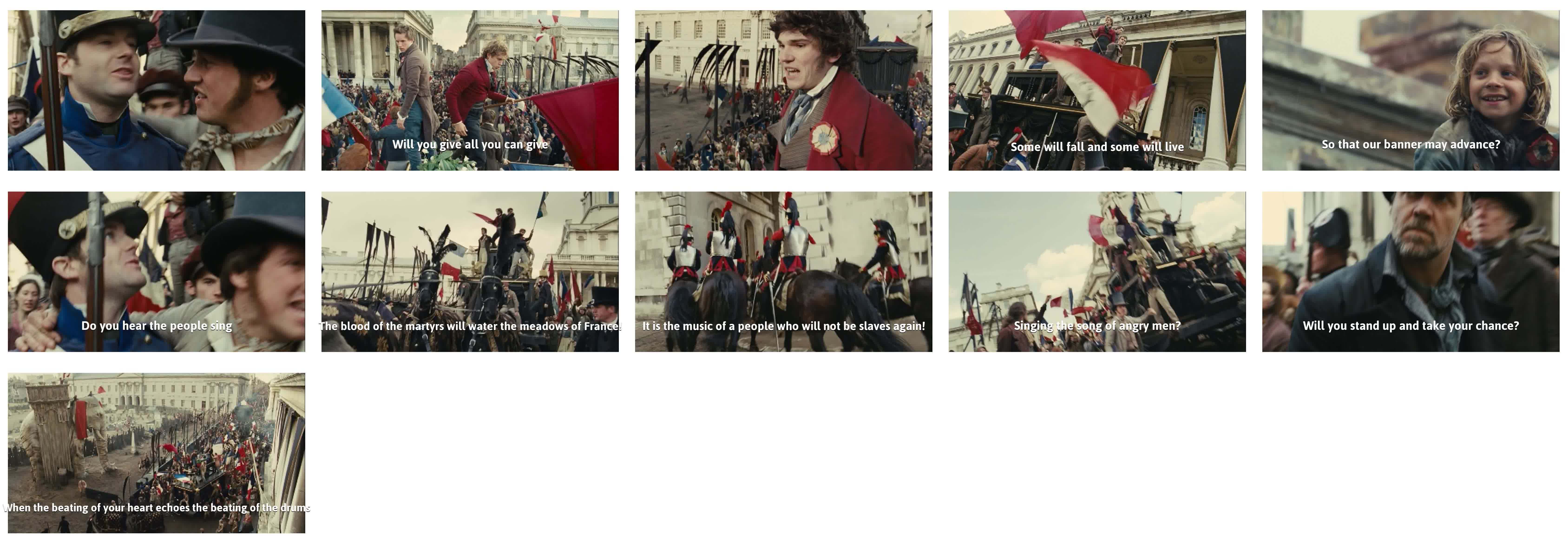
(b) HCMC

(c) Baseline

Figure 16: Movie: Les Misérable. Synopsis: The next day, the students interrupt Lamarque’s funeral procession and begin their assault. Javert poses as a rebel in order to spy on them, but is quickly exposed by Gavroche and captured. During the ensuing gunfight, Eponine saves Marius at the cost of her own life, professing her love to him before she dies, which leaves Marius devastated at the loss of his best friend. Valjean, intercepting a letter from Marius to Cosette, goes to the barricade to protect Marius. After saving Enjolras from snipers, he is allowed to execute Javert. However, when the two are alone, Valjean chooses to free Javert instead and fires his gun to fake the execution. Initially disbelieving, Javert wonders at Valjean’s generosity.

References

- Huang et al. [2020] Qingqiu Huang, Yu Xiong, Anyi Rao, Jiaze Wang, and Dahua Lin. Movienet: A holistic dataset for movie understanding. In European Conference on Computer Vision (ECCV), pages 709–727. Springer, 2020.
- Cohn [2013a] Neil Cohn. Visual narrative structure. Cognitive science, 37(3):413–452, 2013a.
- Frey et al. [2021] Nathan Frey, Peggy Chi, Weilong Yang, and Irfan Essa. Automatic style transfer for non-linear video editing. In Conference on Computer Vision and Pattern Recognition (CVPR), 2021.
- Park et al. [2018] Jungkook Park, Yeong Hoon Park, and Alice Oh. Non-linear editing of text-based screencasts. In ACM Symposium on User Interface Software and Technology (UIST), pages 403–410, 2018.
- Yeung et al. [2016] Serena Yeung, Olga Russakovsky, Greg Mori, and Li Fei-Fei. End-to-end learning of action detection from frame glimpses in videos. In Conference on Computer Vision and Pattern Recognition (CVPR), pages 2678–2687, 2016.
- Feichtenhofer [2020] Christoph Feichtenhofer. X3d: Expanding architectures for efficient video recognition. In Conference on Computer Vision and Pattern Recognition (CVPR), pages 203–213, 2020.
- Fu et al. [2021] Tsu-Jui Fu, Linjie Li, Zhe Gan, Kevin Lin, William Yang Wang, Lijuan Wang, and Zicheng Liu. VIOLET: End-to-end video-language transformers with masked visual-token modeling. In arXiv:2111.1268, 2021.
- Lei et al. [2020] Jie Lei, Licheng Yu, Tamara L Berg, and Mohit Bansal. Tvqa+: Spatio-temporal grounding for video question answering. In Annual Meeting of the Association for Computational Linguistics (ACL), 2020.
- Tapaswi et al. [2016] Makarand Tapaswi, Yukun Zhu, Rainer Stiefelhagen, Antonio Torralba, Raquel Urtasun, and Sanja Fidler. Movieqa: Understanding stories in movies through question-answering. In Conference on Computer Vision and Pattern Recognition (CVPR), June 2016.
- Le and Hoi [2020] Hung Le and Steven CH Hoi. Video-grounded dialogues with pretrained generation language models. arXiv preprint arXiv:2006.15319, 2020.
- Le et al. [2022] Hung Le, Nancy Chen, and Steven Hoi. VGNMN: Video-grounded neural module networks for video-grounded dialogue systems. In North American Chapter of the Association for Computational Linguistics: Human Language Technologies (NAACL-HLT), pages 3377–3393, 2022.
- Wang et al. [2023] Yuxuan Wang, Zilong Zheng, Xueliang Zhao, Jinpeng Li, Yueqian Wang, and Dongyan Zhao. Vstar: A video-grounded dialogue dataset for situated semantic understanding with scene and topic transitions. In Annual Meeting of the Association for Computational Linguistics (ACL), 2023.
- Xu et al. [2015] Kelvin Xu, Jimmy Ba, Ryan Kiros, Kyunghyun Cho, Aaron Courville, Ruslan Salakhudinov, Rich Zemel, and Yoshua Bengio. Show, attend and tell: Neural image caption generation with visual attention. In International Conference on Machine Learning (ICML), pages 2048–2057. PMLR, 2015.
- Anderson et al. [2018] Peter Anderson, Xiaodong He, Chris Buehler, Damien Teney, Mark Johnson, Stephen Gould, and Lei Zhang. Bottom-up and top-down attention for image captioning and visual question answering. In Conference on Computer Vision and Pattern Recognition (CVPR), pages 6077–6086, 2018.
- Cohn [2013b] Neil Cohn. The Visual Language of Comics: Introduction to the Structure and Cognition of Sequential Images. A&C Black, 2013b.
- Zellers et al. [2021] Rowan Zellers, Ximing Lu, Jack Hessel, Youngjae Yu, Jae Sung Park, Jize Cao, Ali Farhadi, and Yejin Choi. Merlot: Multimodal neural script knowledge models. Advances in Neural Information Processing Systems (NeurIPS), 34:23634–23651, 2021.
- Sharma et al. [2020] Vivek Sharma, Makarand Tapaswi, and Rainer Stiefelhagen. Deep multimodal feature encoding for video ordering. arXiv preprint arXiv:2004.02205, 2020.
- Epstein et al. [2021] Dave Epstein, Jiajun Wu, Cordelia Schmid, and Chen Sun. Learning temporal dynamics from cycles in narrated video. In International Conference on Computer Vision (ICCV), pages 1480–1489, 2021.
- Zellers et al. [2019] Rowan Zellers, Yonatan Bisk, Ali Farhadi, and Yejin Choi. From recognition to cognition: Visual commonsense reasoning. In Conference on Computer Vision and Pattern Recognition (CVPR), June 2019.
- Sap et al. [2019] Maarten Sap, Hannah Rashkin, Derek Chen, Ronan LeBras, and Yejin Choi. Socialiqa: Commonsense reasoning about social interactions. arXiv preprint arXiv:1904.09728, 2019.
- Chen et al. [2022] Shixing Chen, Xiang Hao, Xiaohan Nie, and Raffay Hamid. Movies2Scenes: Learning scene representations using movie similarities. arXiv preprint arXiv:2202.10650, 2022.
- Rasheed and Shah [2003] Zeeshan Rasheed and Mubarak Shah. Scene detection in hollywood movies and tv shows. In Conference on Computer Vision and Pattern Recognition (CVPR), volume 2, pages II–343. IEEE, 2003.
- Rao et al. [2020] Anyi Rao, Linning Xu, Yu Xiong, Guodong Xu, Qingqiu Huang, Bolei Zhou, and Dahua Lin. A local-to-global approach to multi-modal movie scene segmentation. In Conference on Computer Vision and Pattern Recognition (CVPR), pages 10146–10155, 2020.
- Chen et al. [2021] Shixing Chen, Xiaohan Nie, David Fan, Dongqing Zhang, Vimal Bhat, and Raffay Hamid. Shot contrastive self-supervised learning for scene boundary detection. In Conference on Computer Vision and Pattern Recognition (CVPR), pages 9796–9805, 2021.
- Shao et al. [2018] Dian Shao, Yu Xiong, Yue Zhao, Qingqiu Huang, Yu Qiao, and Dahua Lin. Find and focus: Retrieve and localize video events with natural language queries. In European Conference on Computer Vision (ECCV), pages 200–216, 2018.
- Radford et al. [2021] Alec Radford, Jong Wook Kim, Chris Hallacy, Aditya Ramesh, Gabriel Goh, Sandhini Agarwal, Girish Sastry, Amanda Askell, Pamela Mishkin, Jack Clark, Gretchen Krueger, and Ilya Sutskever. Learning transferable visual models from natural language supervision. CoRR, abs/2103.00020, 2021.
- Oord et al. [2018] Aaron van den Oord, Yazhe Li, and Oriol Vinyals. Representation learning with contrastive predictive coding. arXiv preprint arXiv:1807.03748, 2018.
- Carreira and Zisserman [2017] Joao Carreira and Andrew Zisserman. Quo vadis, action recognition? a new model and the kinetics dataset. In Conference on Computer Vision and Pattern Recognition (CVPR), pages 6299–6308, 2017.
- Feichtenhofer et al. [2019] Christoph Feichtenhofer, Haoqi Fan, Jitendra Malik, and Kaiming He. Slowfast networks for video recognition. In International Conference on Computer Vision (ICCV), pages 6202–6211, 2019.
- Li et al. [2022] Yanghao Li, Chao-Yuan Wu, Haoqi Fan, Karttikeya Mangalam, Bo Xiong, Jitendra Malik, and Christoph Feichtenhofer. Mvitv2: Improved multiscale vision transformers for classification and detection. In Conference on Computer Vision and Pattern Recognition (CVPR), pages 4804–4814, 2022.
- Lu et al. [2019] Jiasen Lu, Dhruv Batra, Devi Parikh, and Stefan Lee. Vilbert: Pretraining task-agnostic visiolinguistic representations for vision-and-language tasks. Advances in Neural Information Processing Systems (NeurIPS), 32, 2019.
- Li et al. [2019a] Liunian Harold Li, Mark Yatskar, Da Yin, Cho-Jui Hsieh, and Kai-Wei Chang. Visualbert: A simple and performant baseline for vision and language. arXiv preprint arXiv:1908.03557, 2019a.
- OpenAI [2023] OpenAI. Gpt-4 technical report, 2023.
- Tong et al. [2022] Zhan Tong, Yibing Song, Jue Wang, and Limin Wang. Videomae: Masked autoencoders are data-efficient learners for self-supervised video pre-training. arXiv preprint arXiv:2203.12602, 2022.
- Lei et al. [2022] Jie Lei, Tamara L Berg, and Mohit Bansal. Revealing single frame bias for video-and-language learning. arXiv preprint arXiv:2206.03428, 2022.
- Xiong et al. [2019] Yu Xiong, Qingqiu Huang, Lingfeng Guo, Hang Zhou, Bolei Zhou, and Dahua Lin. A graph-based framework to bridge movies and synopses. In International Conference on Computer Vision (ICCV), pages 4592–4601, 2019.
- Cuturi and Blondel [2017] Marco Cuturi and Mathieu Blondel. Soft-DTW: a differentiable loss function for time-series. In International Conference on Machine Learning (ICML), 2017.
- Bengio et al. [2013] Y Bengio, A Courville, and P Vincent. Representation learning: a review and new perspectives. Transactions on Pattern Analysis and Machine Intelligence (TPAMI), 35(8):1798–1828, 2013.
- Tan and Bansal [2019] Hao Tan and Mohit Bansal. LXMERT: Learning cross-modality encoder representations from transformers. In Proceedings of the 2019 Conference on Empirical Methods in Natural Language Processing and the 9th International Joint Conference on Natural Language Processing (EMNLP-IJCNLP), pages 5100–5111, 2019.
- Chen et al. [2019] Yen-Chun Chen, Linjie Li, Licheng Yu, Ahmed El Kholy, Faisal Ahmed, Zhe Gan, Yu Cheng, and Jingjing Liu. UNITER: Learning universal image-text representations. CoRR, 2019.
- Alberti et al. [2019] Chris Alberti, Jeffrey Ling, Michael Collins, and David Reitter. Fusion of detected objects in text for visual question answering. In Proceedings of the 2019 Conference on Empirical Methods in Natural Language Processing and the 9th International Joint Conference on Natural Language Processing (EMNLP-IJCNLP), pages 2131–2140, 2019.
- Yu et al. [2021] Fei Yu, Jiji Tang, Weichong Yin, Yu Sun, Hao Tian, Hua Wu, and Haifeng Wang. Ernie-vil: Knowledge enhanced vision-language representations through scene graphs. In AAAI Conference on Artificial Intelligence (AAAI), volume 35, pages 3208–3216, 2021.
- Gan et al. [2020] Zhe Gan, Yen-Chun Chen, Linjie Li, Chen Zhu, Yu Cheng, and Jingjing Liu. Large-scale adversarial training for vision-and-language representation learning. Advances in Neural Information Processing Systems (NeurIPS), 33:6616–6628, 2020.
- Kenton and Toutanova [2019] Jacob Devlin Ming-Wei Chang Kenton and Lee Kristina Toutanova. Bert: Pre-training of deep bidirectional transformers for language understanding. In North American Chapter of the Association for Computational Linguistics: Human Language Technologies (NAACL-HLT), pages 4171–4186, 2019.
- Alayrac et al. [2020] Jean-Baptiste Alayrac, Adria Recasens, Rosalia Schneider, Relja Arandjelović, Jason Ramapuram, Jeffrey De Fauw, Lucas Smaira, Sander Dieleman, and Andrew Zisserman. Self-supervised multimodal versatile networks. Advances in Neural Information Processing Systems (NeurIPS), 33:25–37, 2020.
- Bain et al. [2021] Max Bain, Arsha Nagrani, Gül Varol, and Andrew Zisserman. Frozen in time: A joint video and image encoder for end-to-end retrieval. In International Conference on Computer Vision (ICCV), pages 1728–1738, 2021.
- Li et al. [2021] Junnan Li, Ramprasaath Selvaraju, Akhilesh Gotmare, Shafiq Joty, Caiming Xiong, and Steven Chu Hong Hoi. Align before fuse: Vision and language representation learning with momentum distillation. Advances in Neural Information Processing Systems (NeurIPS), 34:9694–9705, 2021.
- Yao et al. [2021] Lewei Yao, Runhui Huang, Lu Hou, Guansong Lu, Minzhe Niu, Hang Xu, Xiaodan Liang, Zhenguo Li, Xin Jiang, and Chunjing Xu. Filip: fine-grained interactive language-image pre-training. arXiv preprint arXiv:2111.07783, 2021.
- Alayrac et al. [2022] Jean-Baptiste Alayrac, Jeff Donahue, Pauline Luc, Antoine Miech, Iain Barr, Yana Hasson, Karel Lenc, Arthur Mensch, Katie Millican, Malcolm Reynolds, et al. Flamingo: a visual language model for few-shot learning. arXiv preprint arXiv:2204.14198, 2022.
- Li et al. [2023] Junnan Li, Dongxu Li, Silvio Savarese, and Steven Hoi. Blip-2: Bootstrapping language-image pre-training with frozen image encoders and large language models. arXiv preprint arXiv:2301.12597, 2023.
- Huang et al. [2016] Ting-Hao Huang, Francis Ferraro, Nasrin Mostafazadeh, Ishan Misra, Aishwarya Agrawal, Jacob Devlin, Ross Girshick, Xiaodong He, Pushmeet Kohli, Dhruv Batra, et al. Visual storytelling. In North American Chapter of the Association for Computational Linguistics: Human Language Technologies (NAACL-HLT), pages 1233–1239, 2016.
- Chen et al. [2020] Shizhe Chen, Yida Zhao, Qin Jin, and Qi Wu. Fine-grained video-text retrieval with hierarchical graph reasoning. In Conference on Computer Vision and Pattern Recognition (CVPR), pages 10638–10647, 2020.
- Hou et al. [2020] Jingyi Hou, Xinxiao Wu, Xiaoxun Zhang, Yayun Qi, Yunde Jia, and Jiebo Luo. Joint commonsense and relation reasoning for image and video captioning. In AAAI Conference on Artificial Intelligence (AAAI), volume 34, pages 10973–10980, 2020.
- Yang et al. [2019a] Xu Yang, Kaihua Tang, Hanwang Zhang, and Jianfei Cai. Auto-encoding scene graphs for image captioning. In Conference on Computer Vision and Pattern Recognition (CVPR), pages 10685–10694, 2019a.
- Li et al. [2019b] Linjie Li, Zhe Gan, Yu Cheng, and Jingjing Liu. Relation-aware graph attention network for visual question answering. In International Conference on Computer Vision (ICCV), pages 10313–10322, 2019b.
- Wang et al. [2018] Xiaolong Wang, Ross Girshick, Abhinav Gupta, and Kaiming He. Non-local neural networks. In Conference on Computer Vision and Pattern Recognition (CVPR), pages 7794–7803, 2018.
- Lei et al. [2018] Jie Lei, Licheng Yu, Mohit Bansal, and Tamara L Berg. Tvqa: Localized, compositional video question answering. In EMNLP, 2018.
- Le et al. [2020] Thao Minh Le, Vuong Le, Svetha Venkatesh, and Truyen Tran. Hierarchical conditional relation networks for video question answering. In Conference on Computer Vision and Pattern Recognition (CVPR), pages 9972–9981, 2020.
- Kay et al. [2017] Will Kay, Joao Carreira, Karen Simonyan, Brian Zhang, Chloe Hillier, Sudheendra Vijayanarasimhan, Fabio Viola, Tim Green, Trevor Back, Paul Natsev, et al. The kinetics human action video dataset. arXiv preprint arXiv:1705.06950, 2017.
- Li et al. [2020] Linjie Li, Yen-Chun Chen, Yu Cheng, Zhe Gan, Licheng Yu, and Jingjing Liu. Hero: Hierarchical encoder for video+ language omni-representation pre-training. In Annual Conference on Empirical Methods in Natural Language Processing (EMNLP), pages 2046–2065, 2020.
- Zhu and Yang [2020] Linchao Zhu and Yi Yang. Actbert: Learning global-local video-text representations. In Conference on Computer Vision and Pattern Recognition (CVPR), pages 8746–8755, 2020.
- Vaswani et al. [2017] Ashish Vaswani, Noam Shazeer, Niki Parmar, Jakob Uszkoreit, Llion Jones, Aidan N Gomez, Łukasz Kaiser, and Illia Polosukhin. Attention is all you need. Advances in Neural Information Processing Systems (NeurIPS), 30, 2017.
- Liu et al. [2019] Yinhan Liu, Myle Ott, Naman Goyal, Jingfei Du, Mandar Joshi, Danqi Chen, Omer Levy, Mike Lewis, Luke Zettlemoyer, and Veselin Stoyanov. Roberta: A robustly optimized bert pretraining approach. arXiv preprint arXiv:1907.11692, 2019.
- Yang et al. [2019b] Zhilin Yang, Zihang Dai, Yiming Yang, Jaime Carbonell, Russ R Salakhutdinov, and Quoc V Le. Xlnet: Generalized autoregressive pretraining for language understanding. Advances in Neural Information Processing Systems (NeurIPS), 32, 2019b.
- He et al. [2022] Kaiming He, Xinlei Chen, Saining Xie, Yanghao Li, Piotr Dollár, and Ross Girshick. Masked autoencoders are scalable vision learners. In Conference on Computer Vision and Pattern Recognition (CVPR), pages 16000–16009, 2022.
- Kim et al. [2021] Seonhoon Kim, Seohyeong Jeong, Eunbyul Kim, Inho Kang, and Nojun Kwak. Self-supervised pre-training and contrastive representation learning for multiple-choice video qa. In AAAI Conference on Artificial Intelligence (AAAI), volume 35, pages 13171–13179, 2021.
- Fu* et al. [2023] Tsu-Jui Fu*, Linjie Li*, Zhe Gan, Kevin Lin, William Yang Wang, Lijuan Wang, and Zicheng Liu. An empirical study of end-to-end video-language transformers with masked visual modeling. In Conference on Computer Vision and Pattern Recognition (CVPR), 2023.
- Rohrbach et al. [2015] Anna Rohrbach, Marcus Rohrbach, Niket Tandon, and Bernt Schiele. A dataset for movie description. In Conference on Computer Vision and Pattern Recognition (CVPR), June 2015.
- Gu et al. [2018] Chunhui Gu, Chen Sun, David A. Ross, Carl Vondrick, Caroline Pantofaru, Yeqing Li, Sudheendra Vijayanarasimhan, George Toderici, Susanna Ricco, Rahul Sukthankar, Cordelia Schmid, and Jitendra Malik. AVA: A video dataset of spatio-temporally localized atomic visual actions. In Conference on Computer Vision and Pattern Recognition (CVPR), June 2018.
- Laptev et al. [2008] Ivan Laptev, Marcin Marszalek, Cordelia Schmid, and Benjamin Rozenfeld. Learning realistic human actions from movies. In Conference on Computer Vision and Pattern Recognition (CVPR), pages 1–8, 2008. doi: 10.1109/CVPR.2008.4587756.
- Bhattacharya et al. [2014] Subhabrata Bhattacharya, Ramin Mehran, Rahul Sukthankar, and Mubarak Shah. Classification of cinematographic shots using lie algebra and its application to complex event recognition. IEEE Transactions on Multimedia, 16(3):686–696, 2014. doi: 10.1109/TMM.2014.2300833.
- Vicol et al. [2018] Paul Vicol, Makarand Tapaswi, Lluis Castrejon, and Sanja Fidler. MovieGraphs: Towards understanding human-centric situations from videos. In Conference on Computer Vision and Pattern Recognition (CVPR), 2018.
Supplementary Materials