Sen2Pro: A Probabilistic Perspective to Sentence Embedding
from Pre-trained Language Model

Abstract

Sentence embedding is one of the most fundamental tasks in Natural Language Processing and plays an important role in various tasks. The recent breakthrough in sentence embedding is achieved by pre-trained language models (PLMs). Despite its success, an embedded vector (Sen2Vec) representing a point estimate does not naturally express uncertainty in a task-agnostic way. This paper thereby proposes an efficient framework on probabilistic sentence embedding (Sen2Pro) from PLMs, and it represents a sentence as a probability density distribution in an embedding space to reflect both model uncertainty and data uncertainty (i.e., many-to-one nature) in the sentence representation. The proposed framework performs in a plug-and-play way without retraining PLMs anymore, and it is easy to implement and generally applied on top of any PLM. The superiority of Sen2Pro over Sen2Vec has been theoretically verified and practically illustrated on different NLP tasks.

1 Introduction

Sentence embedding, which maps an input sentence to a point (i.e., a vector) in an embedded space, is one of the most fundamental tasks in Natural Language Processing (NLP), and it plays an important role in various downstream tasks such as sentiment analysis, text classification, and natural language inference Howard and Ruder (2018); Reimers and Gurevych (2019); Gao et al. (2021). There is a surge of interest in learning sentence embedding. The early work resorts to word embedding Bengio et al. (2003); Mikolov et al. (2013); Pennington et al. (2014) and represents an input sentence by a pooling vector (mean or weighted mean) over all embeddings of its words Kiros et al. (2015); Wieting et al. (2015a). More recently, sentence embedding obtained from pre-trained language models (PLMs) made a breakthrough thanks to PLM’s powerful ability in modeling global context Peters et al. (2018); Devlin et al. (2019); Liu et al. (2019), and it quickly became the standard practice for sentence embedding.

Despite the success of sentence embedding from PLMs, an embedded vector (Sen2Vec) representing a point estimate does not naturally express uncertainty about the target concepts associated with the input sentence Vilnis and McCallum (2015). In essence, this uncertainty originates from many-to-one nature in language representation: (1) model uncertainty: model uncertainty refers to the notion of randomness caused by inherently random effects within the model. (i.e. one sentence may have many representations according to different representations within the same model (e.g., dropout)) Considering that these representation are from the same sentence, they should remain close to each other; (2) data uncertainty: many sentences with different linguistic structure (e.g., paraphrase) may have the same meaning in semantics. Considering the identical semantics, their corresponding representation should get close with each other.

When quantifying uncertainty, we assume that close-semantic sentences’ representation follows the same probability distribution. Given a sentence, since the model only observes one sample, it is natural to ask how much a language model can capture such a rich distribution.

A natural solution to this issue is to merge such a probabilistic perspective into sentence embedding, which represents a sentence as a distribution $P(\mu,\Sigma)$, where $\mu$ is the mean and covariance $\Sigma$ intuitively portrays the uncertainty of the distribution $P$. Unfortunately, there is a critical challenge to putting this idea into practice: previous works Bamler and Mandt (2017); Camacho-Collados and Pilehvar (2018); Zhou et al. (2019) are only plausible on word embedding and require retraining word embedding with probabilistic embedding on large-scale data to advance SOTA. It is costly even for training a PLM without probabilistic embedding Devlin et al. (2019); Radford et al. (2019); He et al. (2020); Clark et al. (2019); Raffel et al. (2020), which typically consumes considerable GPU computations for weeks.

In this paper, we propose an efficient framework for probabilistic sentence embedding (Sen2Pro) from PLMs that represents a sentence as a probability density in an embedding space to reflect the uncertainty in the sentence representation.

Concerning model uncertainty and data uncertainty, we propose two simple methods to quantify both on top of a PLM. Specifically, to measure model uncertainty, we assume a sentence vector is drawn from a distribution $P(\mu^{m},\Sigma^{m})$, which can be estimated by many representations of the targeted sentence using a set of stochastic PLMs obtained from Monte Carlo dropout Gal and Ghahramani (2016).

Similarly, we apply the data augmentation technique to generate many semantically equivalent sentences to the targeted sentence for measuring data uncertainty. Then we assume a sentence vector is drawn from a distribution $P(\mu^{d},\Sigma^{d})$, which the representations of the augmented sentences from the PLM can estimate. In addition, we also introduce some ways to utilize both $\mu^{m}$ ($\mu^{d}$) and $\Sigma^{m}$ ($\Sigma^{d}$) as the final sentence representation for different downstream tasks.

Moreover, drawing from previous works Chen et al. (2016); Li and Chen (2019); Gao et al. (2019); Tschannen et al. (2019); Grohs et al. (2021) that explored the relationships between deep learning representation and relative entropy, we present theoretical explanations of why our probabilistic sentence embedding (Sen2Pro) is superior to point vector-based sentence embedding (Sen2Vec). Meanwhile, extensive experiments demonstrate the practical effectiveness of Sen2Pro on text classification, semantic similarity match, dialogue generation evaluation, and machine translation evaluation. Besides, Sen2Pro demonstrates its superiority in capturing sentence-level linguistic analogy over Sen2Vec.

2 Related Work

2.1 Sentence Embedding

Methods for sentence embedding learning have been extensively explored, and all these methods represent a sentence as a point embedding. Early works use the weighted sum of word embedding to represent a sentence. Then some methods based on the distributional hypothesis have been done. Hill Hill et al. (2016) learned sentence representations with the internal structure of each sentence, and Kiros Kiros et al. (2015) followed the idea of Word2Vec Mikolov et al. (2013) to represent a sentence by predicting its surrounding sentences. In recent years, the pre-trained language model Devlin et al. (2019) has become the standard sentence paradigm because of its strong ability to capture syntactic and semantic features of sentences by learning from the large-scale corpus. Furthermore, several researchers used contrastive learning to augment sentence representation Zhang et al. (2020); Yan et al. (2021); Meng et al. (2021); Gao et al. (2021); Wang et al. (2021), based on the assumption that a high-quality representation method should bring similar sentences closer while pushing away dissimilar ones. They belong to Sen2Vec and thus fail to model uncertainty. This paper goes beyond point sentence embedding and explores probabilistic sentence embedding.

2.2 Probabilistic Word Embedding

In NLP, probabilistic embedding originated from word embedding Bengio et al. (2003); Mikolov et al. (2013), and existing probabilistic embedding methods work only on words, where a word from the vocabulary is represented as a density distribution in an embedding space. Although variants of probabilistic word embedding have been developed Vilnis and McCallum (2015); Bamler and Mandt (2017); Camacho-Collados and Pilehvar (2018); Zhou et al. (2019), they used a similar paradigm, which adapts the Skip-gram model Mikolov et al. (2013) with a non-parametric approach. Specifically, a Skip-gram model is retrained as the density distribution with a specific word sampling (e.g., synonym) method and a specific loss function (e.g., a margin loss). Therefore, existing probabilistic embedding needs an extremely time-consuming retraining stage and can not be applied to PLMs (e.g., BERT). Different from them, this paper contributes to the literature by developing probabilistic embedding for sentences that serves as a plug-and-play method on pre-trained language models Devlin et al. (2019) without any time-consuming retraining stage.

3 Methodology: Sen2Pro

Because of the many-to-one nature of sentence embedding, we model the uncertainty from two perspectives, i.e., model uncertainty and data uncertainty. Accordingly, we assume that the representation of one sentence follows a distribution $P(\mu,\Sigma)$, which measures either model uncertainty or data uncertainty. The goal of our Sen2Pro framework is to estimate the two distributions $P(\mu,\Sigma)$ for a sentence embedding based on a pre-trained language model $f_{\theta}$ (e.g., BERT), where $\theta$ denotes its parameters. In general, there are two steps in Sen2Pro: the sampling stage and the estimation stage. The sampling stage generates embedding instances to capture two kinds of uncertainties: model uncertainty and data uncertainty (§3.1). The estimation stage aims to estimate the parameters in the density distributions (i.e., mean vector and covariance matrix) based on the embedding instances (§3.2). After both distributions are estimated, the general idea to apply them to specific tasks is presented (§3.3).

3.1 Sampling Stage

Model Uncertainty

Model uncertainty originates from the fact that one sentence may have different representations due to inherent randomness within models. In this paper, we use a pre-trained language model $f_{\theta}$ and try to quantify model uncertainty. Considering that the key ingredient of model uncertainty is to vary the model while keeping the sentence $s$ unchanged, we utilize MC dropout to create embedding instances for quantifying model uncertainty. Specifically, for each sentence ${s}$, we utilize MC Dropout Gal and Ghahramani (2016); Lakshminarayanan et al. (2017) over the parameters $\theta$ as sampling, and repeat sampling $N$ times to obtain different subsets of the parameters $\theta$: $\{\widehat{\theta}_{i}\mid i=1,\ldots,N\}$. In this way, we generate a set of embeddings as follows:

$$\mathcal{S}^{m}=\big{\{}x_{i}=f_{\widehat{\theta}_{i}}\left(s\right)\mid i=1,\ldots,N\big{\}}$$ (1)

As shown in Eq. 1, each subset of model’s parameters represent a sub-structure of the model, which naturally matches with the definition of model uncertainty.

Data Uncertainty

Data uncertainty corresponds to the many-to-one nature of sentence embedding. In other words, sentences that are semantically similar but slightly different should have close representations. Data uncertainty exists in universal real-world scenarios: since the model requires lots of training data to perform well, it is common to augment high-quality labeled sentences with lower-quality web-crawled data to save time and effort. To naturally imitate such uncertainty, in this paper, a simple data augmentation method, word-level operation, is applied to the input sentence, which adds proper noise to an input sentence. After repeating data augmentation $N$ times (i.e., randomly dropping a word in ${s}$, swapping two words, replacing or inserting a word in ${s}$ with any word from vocabulary) for the input sentence $s$, a set of new sentences, $s_{1},s_{2},\ldots,s_{N}$ are obtained. Then, the sentences are fed to the pre-trained model $f_{\theta}$ to get $N$ embeddings. In this way, we can obtain a set of embeddings as follows:

$$\mathcal{S}^{d}=\big{\{}x_{i}=f_{\theta}\left(s_{i}\right)\mid i=1,\ldots,N\big{\}}$$ (2)

3.2 Estimation Stage

After obtaining the required embedding instances for model and data uncertainty, we can estimate the probability distributions on them, respectively. Similar to cases of Kendall and Gal (2017); Maddox et al. (2019); Ovadia et al. (2019); Abdar et al. (2021); Hüllermeier and Waegeman (2021), we do estimation towards two uncertainty individually rather than unifying, which is also empirically verified in Appendix D. Suppose $\mathcal{S}$ denotes either $\mathcal{S}^{m}$ or $\mathcal{S}^{d}$, it is natural to estimate its mean and covariance as follows:

$$\mu=\frac{1}{|\mathcal{S}|}\sum_{x\in\mathcal{S}}x$$ (3)

$$\Sigma=\frac{1}{|\mathcal{S}|}\sum_{x\in\mathcal{S}}(x-\mu)(x-\mu)^{\top}$$ (4)

where $|\mathcal{S}|$ means the size of the set $\mathcal{S}$ and $(.)^{\top}$ is an transpose operation. We use $\mu^{m}$ and $\Sigma^{m}$ respectively to denote the statistics estimated from model uncertainty (i.e., $\mathcal{S}=\mathcal{S}_{m}$), and $\mu^{d}$ and $\Sigma^{d}$ denote those estimated through data uncertainty (i.e., $\mathcal{S}=\mathcal{S}_{d}$).

However, such a simple covariance matrix estimator (SCE) owns severe problems on both theoretical Xiao and Wu (2012) and practical sides: it is known to degrade rapidly as an estimator as the number of variables increases, thus performing badly in a high-dimensional case (e.g., 768 dimensions in BERT). To address this issue, inspired by Bien et al. (2016), we instead employ the banding estimator, which uses an off-diagonal entry removal operation on the covariance matrix.

Specifically, for a covariance matrix $\Sigma=\left(\Sigma_{ij}\right)_{k\times k}$ where $k$ is the dimension of $\Sigma$, we use $B(\Sigma)$ as the estimation of $\Sigma$ as follows:

$$\hat{\Sigma}=B(\Sigma)=\operatorname{Diag}(\Sigma)$$ (5)

Besides, Theorem 1 provides an estimation error bound for our banding estimator, whose proof is presented in Appendix A.

Theorem 1.

Suppose $\Sigma$ is the covariance matrix of the ground truth distribution $P(\mu,\Sigma)$, and $\hat{\Sigma}$ denote $B(\Sigma)$, then we have

$$\left\|\hat{\Sigma}-{\Sigma}\right\|_{2}=O_{p}\left(\left(\frac{\log k}{n}\right)^{M}\right)$$ (6)

where $k$ is the dimension of $\Sigma$, and $M$ is a positive constant satisfying $M<\frac{1}{2}$. $O_{p}$ and $n$ means $\frac{\log k}{n})^{M}$ is stochastically bounded as $n\to\infty$.

Besides, SCE also in practicability problems compared to the banding estimator. SCE owns a significantly worse performance-efficiency trade-off than our banding estimator, which will be empirically verified in Sec 5. Moreover, theoretical analyses for comparison between Sen2Vec and Sen2Pro are deferred to Appendix B.

3.3 Usage of Sen2Pro

Unlike previous works on probabilistic embedding that drop $\hat{\Sigma}$ in tasks, in Sen2Pro, both mean vector $\mu$ (i.e., $\mu^{m}$ and $\mu^{d}$) and covariance vector $\hat{\Sigma}$ (i.e., $\hat{\Sigma}^{m}$ and $\hat{\Sigma}^{d}$) are used for sentence embedding. In the next section, we illustrate our strategies to use $\mu$ and $\hat{\Sigma}$, more details are presented in Sec 4.1.

Dataset	Model	10	200	Full	Dataset	Model	10	200	Full
AGNews	BERT-base	69.5	87.5	95.2	DBPedia	BERT-base	95.2	98.5	99.3
	BERT-base-G	74.4(1.1)	90.2(0.3)	95.6(0.1)		BERT-base-G	96.5(0.2)	99.1(0.1)	99.3(*)
Yahoo	BERT-base	56.2	69.3	77.6	IMDB	BERT-base	67.5	86.9	95.6
	BERT-base-G	60.5(1.8)	72.9(0.6)	78.2(0.2)		BERT-base-G	70.4(0.6)	88.5(0.3)	95.7(*)

Table 1: Test accuracy(%) comparison between Sen2Pro and Sen2Vec for text classification. The results on each dataset are the mean of three runs; the standard derivation (i.e., the values in brackets) is given for PLM-G, where * means the derivation is smaller than 0.1%.

4 Experiment

Baseline	STS-12	STS-13	STS-14	STS-15	STS-16	Avg
BERT	57.86$\rightarrow$59.55	61.97$\rightarrow$66.20	62.49$\rightarrow$65.19	70.96$\rightarrow$73.50	69.76$\rightarrow$72.10	63.69$\rightarrow$66.70(+3.01)
BERTl	57.74$\rightarrow$59.90	61.16$\rightarrow$66.20	61.18$\rightarrow$65.62	68.06$\rightarrow$73.01	70.30$\rightarrow$74.72	62.62$\rightarrow$67.47(+4.85)
W-BERT	63.62$\rightarrow$64.50	73.02$\rightarrow$73.69	69.23$\rightarrow$69.69	74.52$\rightarrow$74.69	72.15$\rightarrow$76.11	69.21$\rightarrow$70.39 (+1.18)
W-BERT	64.02$\rightarrow$64.90	73.27$\rightarrow$73.94	69.58$\rightarrow$70.04	74.77$\rightarrow$74.94	72.50$\rightarrow$76.44	69.58$\rightarrow$70.69 (+1.26)
C-BERT	64.09$\rightarrow$65.01	78.21$\rightarrow$78.54	68.68$\rightarrow$69.04	79.56$\rightarrow$79.90	75.41$\rightarrow$75.74	72.27$\rightarrow$72.69 (+0.42)
C-BERTl	70.23$\rightarrow$70.70	82.13$\rightarrow$82.54	73.60$\rightarrow$74.12	81.72$\rightarrow$82.01	77.01$\rightarrow$77.58	76.03$\rightarrow$76.48 (+0.45)
Sim-BERT	68.93$\rightarrow$69.33	78.68$\rightarrow$78.93	73.57$\rightarrow$73.95	79.68$\rightarrow$80.01	79.11$\rightarrow$79.29	75.11$\rightarrow$75.44 (+0.33)
Sim-BERTl	69.25$\rightarrow$69.60	78.96$\rightarrow$79.30	73.64$\rightarrow$73.92	80.06$\rightarrow$80.31	79.08$\rightarrow$79.42	75.31$\rightarrow$75.61 (+0.30)

Table 2: The experimental results of adding our Sen2Pro on widely used sentence embedding methods. Specifically, BERT_l means BERT_large.

Sentence Embedding	MRR	Hits@1	Hits@3
BERT	68.01	51.70	81.91
BERT+Ours	68.69	52.24	82.63
BERT-whitening	66.58	46.54	84.22
BERT-whitening+Ours	67.49	48.23	84.56
Sentence-BERT	64.12	47.07	79.05
Sentence-BERT+Ours	66.10	48.55	80.34
SimCSE	69.50	52.34	84.43
SimCSE+Ours	70.01	52.68	84.69

Table 3: Performances on EvalRank Wang et al. (2022) using Sen2Vec and Sen2Pro. ‘+Ours’ means Sen2Pro, and the results are the mean of five runs to show the statistical significance with $p$ value <0.05.

This section comprehensively evaluates the effectiveness of our Sen2Pro framework on the following various tasks. The results consistently show that Sen2Pro outperforms Sen2Vec. Specifically, we choose two sets of tasks for evaluation: Fine-tune-need Task and Fine-tune-free Task.

4.1 Basic Setting

Recall that $\mu^{m}$ and $\hat{\Sigma}^{m}$ ($\mu^{d}$ and $\hat{\Sigma}^{d}$) denote the estimated mean and covariance from model (data) uncertainty. Then we present how to use them for different tasks.

Fine-tune-need Task: Text Classification

After estimation stage in data and model uncertainty, each sentence is represented as the concatenation of $\frac{\mu^{m}+\mu^{d}}{2}$ and (diagonal entries of) $\frac{\hat{\Sigma}^{m}+\hat{\Sigma}^{d}}{2}$. Specifically, we use reparameterization to handle the non-differentiable issue of the sampling process.

Fine-tune-free Task: Sentence Similarity, Dialogue Evaluation, Neural Machine Translation Evaluation

For such NLP tasks, the distance between two representations is needed. Although KL divergence is natural to measure the distance between two distributions, it has practical drawbacks. For example, in BERT-base case where $\mu\in\mathcal{R}^{768\times 1}$, $\hat{\Sigma}\in\mathcal{R}^{768\times 768}$, KL divergence not only is time-consuming but also results in numerical errors, considering that KL divergence includes operations $det(\hat{\Sigma})$ and $\hat{\Sigma}^{-1}$. In practice, most entries of $\hat{\Sigma}$ are between 0 and 0.5, so the determinant becomes extremely small, which leads to numerical errors. Moreover, the computation of $\hat{\Sigma}^{-1}$ will be unstable when the dimension is high.

Therefore, a simple function is taken to measure the distance between two probabilistic sentence embeddings $(\mu_{a},\Sigma_{a})$ and $(\mu_{b},\Sigma_{b})$ as follows:

$$d(\mathcal{N}(\mu_{a},\Sigma_{a}),\mathcal{N}(\mu_{b},\Sigma_{b}))$$ (7)

$$=(1-\alpha)l_{1}(\mu_{a}-\mu_{b})+\alpha l_{1}(\Sigma_{a}-\Sigma_{b})$$

where $l_{1}$ represents the $l_{1}$-norm and $\alpha$ is to balance the two terms. For $\alpha$, we consider it as a balance factor for different magnitudes of $\mu$ and $\Sigma$, defined as follows:

$$\alpha=\frac{l_{1}(\mu_{a}-\mu_{b})}{l_{1}(\Sigma_{a}-\Sigma_{b})}$$ (8)

In most cases, $\alpha$ ranges from 0.01 to 0.05. Besides, we will try to apply Sen2Pro on other evaluation tasks Shen et al. (2022a, b) like paraphrase, data-to-text, and summarization.

4.2 Text Classification

Benchmarks and Setting

We choose four widely-used text classification benchmarks: AG News Zhang et al. (2015), DBpedia Maas et al. (2011), Yahoo! Answers Chang et al. (2008) and IMDB Maas et al. (2011). The evaluation metric is the test accuracy, and the best performance is selected based on validation set accuracy. The baseline is Sen2Vec, with 15 data augmentation samples per sentence. In Sen2Pro, we choose the BERT-base model as the PLM and use the ‘first-last-avg’(a pooling way that average first and last layer representation). The sampling number is 15 for the model uncertainty and data uncertainty. Moreover, we use two settings for model evaluation: few-shot and full-dataset. In the few-shot setting, models are trained with randomly selected 10 and 200 labeled sentences per class. In the full-dataset setting, models are trained with the whole training set.

Performances

The results are listed in Table 1. Our Sen2Pro consistently performs better than Sen2Vec under few-shot settings because Sen2Pro contains more semantic information about a sentence due to its probabilistic characteristic. Moreover, Sen2Pro achieves comparable or better performances in the full training setting than Sen2Vec.

4.3 Sentence Similarity

Benchmarks and Setting

We use seven commonly-used STS datasets Agirre et al. (2012, 2013, 2014, 2015, 2016) for evaluation. Besides, considering the limitation of traditional intrinsic evaluation Wang et al. (2022), we choose EvalRank Wang et al. (2022) for linguistic analogy evaluation, which overcomes the previous limitation. In Sen2Pro, we use several state-of-the-art pre-trained language models, including BERT-base Devlin et al. (2019), BERT-whitening Su et al. (2021); Huang et al. (2021), Sentence-BERT Reimers and Gurevych (2019), and SimCSE Gao et al. (2021). Specifically, EvalRank uses the mean reciprocal rank (MRR) and Hits@k scores for evaluation, and a higher score indicates a better embedding model. The sampling number for each uncertainty is set as 15.

Performances

The results of Sen2Pro are reported in Table 2 and  3, which illustrate that Sen2Pro outperforms Sen2Vec with a substantial gap under all settings. Moreover, Sen2Pro using the‘base’ PLMs can achieve better or comparable performance than Sen2Vec using ‘large’ PLMs.

Metric	Daily(H)		Convai2		Empathetic
	Spr	Pr	Spr	Pr	Spr	Pr
BLEU	44.5	44.4	80.0	80.1	13.6	33.1
METEOR	1.8	5.0	80.0	76.7	38.2	13.3
ROUGE-L	54.5	41.7	20.0	6.1	39.1	47.2
Greedy	85.5	76.4	60.0	79.4	73.6	86.4
Average	20.9	20.9	60.0	87.9	66.4	72.5
Extrema	74.5	76.1	80.0	76.6	61.8	72.2
B-SCORE	85.5	85.7	80.0	93.9	60.0	69.7
Sen2Vec	69.9	76.1	60.0	63.9	55.2	60.3
Sen2Pro	87.3	81.4	100	85.9	80.9	81.6

Table 4: Correlations of the evaluation metrics on the dialogue corpora. ‘Spr.’ and ‘Pr.’ refer to Spearman and Pearson correlation coefficients, respectively; B-SCORE represents BERTScore.

Metric	cs-en	de-en	fi-en	lv-en	ru-en	tr-en	zh-en	Avg
BLEU	97.1	92.3	90.3	97.9	91.2	97.6	86.4	93.3
CDER	98.9	93.0	92.7	98.5	92.2	97.3	90.4	94.7
BLEND	96.8	97.6	95.8	97.9	96.4	98.4	89.4	96.0
BERTScore	99.6	98.2	94.7	97.9	956	98.6	98.4	97.6
Sen2Vec	97.3	92.5	93.1	98.6	90.1	98.0	92.1	94.5
Sen2Pro	99.8	96.2	99.0	99.5	96.5	99.0	97.9	97.8

Table 5: Pearson correlations with system-level machine translation evaluation on WMT17.

4.4 Dialogue Evaluation

Benchmark and Setting

We choose three widely-used dialogue benchmarks: Daily(H) Lowe et al. (2017), Convai2 Dinan et al. (2020), and Empathetic Rashkin et al. (2019). Each benchmark consists of dialogue queries, the corresponding responses, and human-annotated responses. For baseline metrics, we choose BLEU Papineni et al. (2002), ROUGE Lin (2004), METEOR Denkowski and Lavie (2014), Greedy Matching Rus and Lintean (2012), Embedding Average Wieting et al. (2015b), Vector Extrema Forgues et al. (2014) and BERTScore Zhang et al. (2019). For Sen2Pro, we use the BERT-base model and the ‘first-last-avg’ representation and set the sampling number of uncertainty to 15.

Performances

The performances of various evaluation metrics are reported in Table 4. Sen2Pro performs best in most cases, demonstrating its good generalization ability and robustness for the dialogue evaluation task.

Model	STS-12	STS-13	STS-14	STS-15	STS-16	STS-B	SICK-R	Average
BERT-base	57.84	61.95	62.48	70.95	69.81	59.04	63.75	63.69
BERT-base-$G_{m+d}$	59.40	63.03	64.18	71.97	70.73	62.59	64.69	65.23 (+1.54)
BERT-base-$G_{m}$	58.86	62.66	63.77	71.48	70.56	61.89	64.28	64.79 (+1.10)
BERT-base-$G_{d}$	58.14	62.20	62.83	71.00	70.36	59.30	64.10	63.99 (+0.30)

Table 6: Ablation studies on the two uncertainties in STS. BERT-base-$G_{m}$ and BERT-base-$G_{d}$ represent Sen2Pro with only model uncertainty or data uncertainty, respectively.

4.5 NMT Evaluation

Benchmark and Setting

We work on the WMT-17 machine translation benchmark Bojar et al. (2017). Moreover, BLEU Papineni et al. (2002), CDER Leusch et al. (2006), BLEND Ma et al. (2017), Sen2Vec, and BERTScore Zhang et al. (2019) are chosen as baseline metrics. The setting of Sen2Pro is the same as the one of dialogue evaluation.

Performances

The results are shown in Table 5. Our Sen2Pro achieves comparable performance towards a top metric (i.e., BERTScore) and significantly outperforms Sen2Vec, which demonstrates the effectiveness of Sen2Pro in the NMT evaluation task. Segment-level results are shown in Appendix H. The results indicate that our Sen2Pro can yield competitive performance to SOTA as an automatic metric to evaluate dialogue generation.

5 Analysis and Discussion

This section presents analyses of Sen2Pro, and the BERT model is used as the PLM in the analyses. Specifically, the representation uncertainty analysis is made on the STS task, and detailed results are deferred to Appendix E and F. Moreover, we choose the BERT model as our pre-trained sentence encoder in the analysis.

Feature with higher model uncertainty is more important

We investigate the relation between the model uncertainty and the feature importance on the STS task. In Sen2Pro, a sentence is represented as $\mu^{m}\in\mathcal{R}^{768\times 1}$ and diagonal entries of $\hat{\Sigma}^{m}\in\mathcal{R}^{768\times 768}$. From another perspective, a sentence is represented by 768 features in $\mu^{m}$, and $\hat{\Sigma}^{m}$ reflects the corresponding model uncertainties of such features. Let $T$ be the feature set, and $t\in T$ is a feature subset. We define the feature importance as follows:

$$score(t)=|\rho(T)-\rho(T/t)|$$ (9)

where $\rho$ represents Spearman’s correlation in STS evaluation, and $score(t)$ describes the performance change after removing the feature subset $t$ from $T$. Then we separate the 768 features into five groups according to their uncertainty $\hat{\Sigma}^{m}$, and name them as ‘I’ to ‘V’, as shown in Figure 1. When a group of features is removed from $T$, these features are set to 0 in $\mu^{m}$ and $\hat{\Sigma}^{m}$, respectively. Figure 1 lists the results on STS-12. In Figure 1, as the feature’s uncertainty decreases, the importance score drops, indicating that features with higher uncertainty are more important in the STS task.

Figure 1: The importance score of five groups of features. ‘I’ represents the features with top 20% highest uncertainty; ‘V’ indicates the features with bottom 20% lowest uncertainty; ‘Min’ and ‘Max’ mean the lowest and highest importance score under three runs.

Dataset	Model	10	200	Full	Dataset	Model	10	200	Full
AGNews	BERT-base	69.5	87.5	95.2	DBPedia	BERT-base	95.2	98.5	99.3
	BERT-base-G	73.4(0.5)	89.2(0.3)	95.4(0.1)		BERT-base-G	96.3(0.2)	99.1(0.1)	99.3(*)
	BERT-base-$G_{m}$	71.6(1.0)	88.3(0.4)	95.2(0.2)		BERT-base-$G_{m}$	95.8(0.2)	98.8(*)	99.3(*)
	BERT-base-$G_{d}$	73.0(0.4)	89.0(0.3)	95.4(0.1)		BERT-base-$G_{d}$	96.3(0.3)	99.1(0.1)	99.3(*)
Yahoo	BERT-base	56.2	69.3	77.6	IMDB	BERT-base	67.5	86.9	95.6
	BERT-base-G	60.1(0.8)	72.4(0.6)	78.0(0.1)		BERT-base-G	70.3(0.6)	88.2(0.3)	95.7(*)
	BERT-base-$G_{m}$	58.1(1.0)	70.3(0.5)	77.9(*)		BERT-base-$G_{m}$	69.2(0.6)	87.5(0.2)	95.6(*)
	BERT-base-$G_{d}$	59.9(0.7)	71.7(0.3)	78.0(0.1)		BERT-base-$G_{d}$	69.8(0.4)	88.2(0.1)	95.7(*)

Table 7: Ablation studies on the two uncertainties in text classification.

Sen2Pro brings more benefits when model uncertainty are higher

We also investigate the relation between the model uncertainty and the performance improvement of Sen2Pro over Sen2Vec on the STS task. Firstly, we define a metric called Fluctuation Rate $Q$ as follows:

$$Q(f,D)=\frac{\Sigma_{i=1}^{|D|}(\Sigma_{j=1}^{k}\sigma_{ij})}{k\times|D|}$$ (10)

where $f$ and $D$ represent the PLM and benchmark, and $\sigma_{ij}$ is $j$-th element of the covariance matrix for $i$-th sentence in $D$, and $k$ denotes the dimension of model $f$. Such a metric can generally reflect the uncertainty of a specific model towards a specific benchmark. Based on $Q(f,D)$, we define the improvement score $I$ reflecting the improvement of Sen2Pro over Sen2Vec as follows:

$$I=P_{Sen2Pro}(f,D)-P_{Sen2Vec}(f,D)$$ (11)

where $P_{Sen2Pro}(f,D)$ and $P_{Sen2Vec}(f,D)$ represent the performance of model $f$ on $D$ under Sen2Pro and Sen2Vec, respectively. Besides, we add the result of [CLS] representation into experiments since the [CLS] representation owns a significantly higher fluctuation rate than the ‘first-last-avg’ representation. The results on STS-12 are illustrated in Figure 2. As the fluctuation rate increases, the improvement score becomes more significant. Such empirical results demonstrate that the effectiveness of Sen2Pro is highly correlated to the model uncertainty and show Sen2Pro’s superiority over Sen2Vec owns a positive correlation to model uncertainty.

Figure 2: The relation between fluctuation rate ($Q$) and improvement score ($I$). ‘-b’ and ‘-l’ indicate ‘base’ and ‘large’, and ‘Avg’ and ‘CLS’ represent the ‘first-last-avg’ and ‘[CLS]’ representation.

Effectiveness of Two Uncertainties

We verify the effect of model and data uncertainty on Sen2Pro’s performances. Specifically, Sen2Pro is evaluated on one intrinsic evaluation (STS) and one downstream task (text classification), and the results are demonstrated in Table 6 and Table 7, respectively. As shown in Table 6, the performance decreases when the data uncertainty is applied alone for the STS task since sentences’ semantics may be changed due to the data augmentation. In contrast, the model uncertainty consistently brings benefits to the sentence representation. For text classification, both uncertainties improve the representation’s generalization. Specifically, the contribution of the data uncertainty is higher than the model uncertainty. These empirical results also illustrate the usage of Sen2Pro (§3.3).

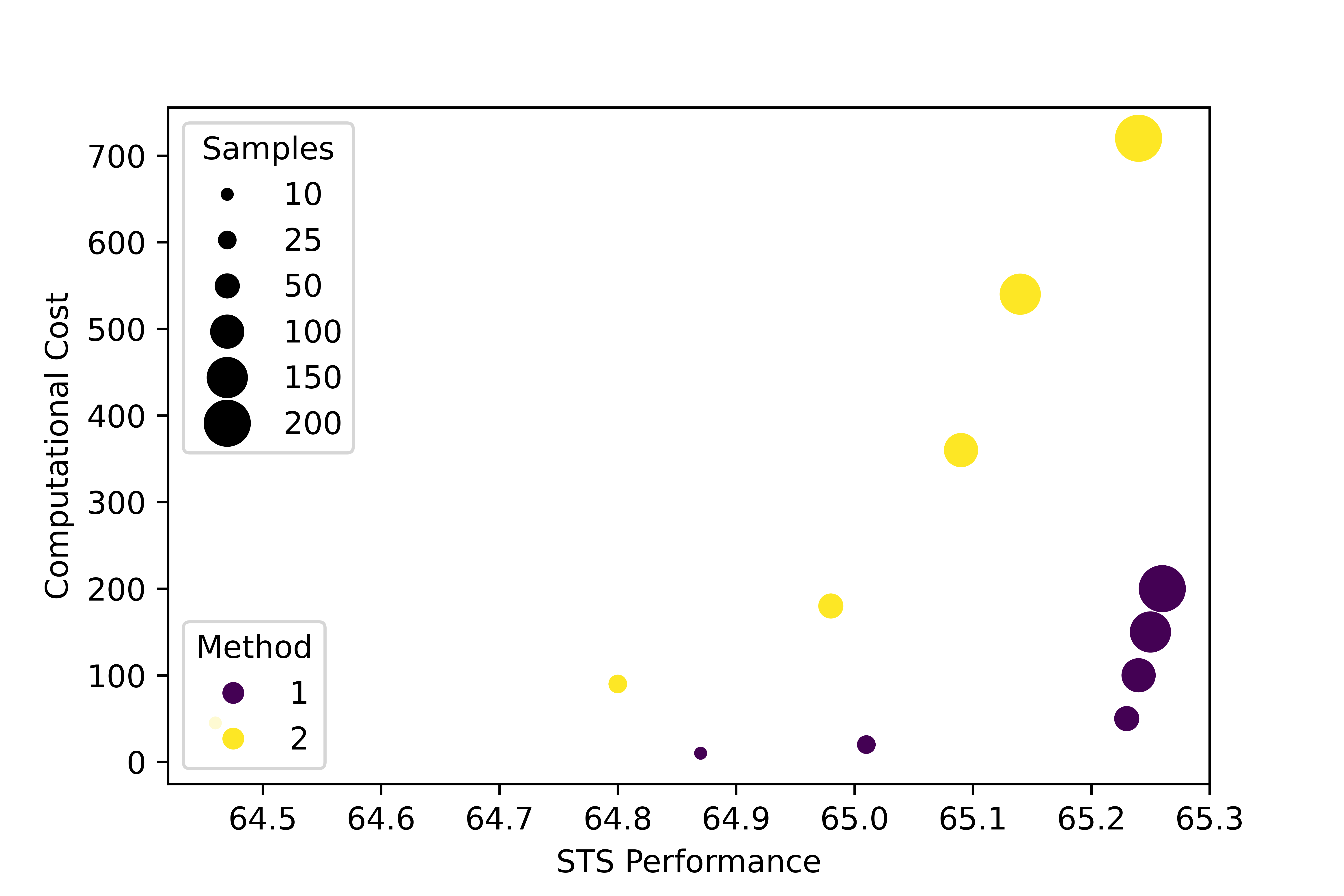
Figure 3: The performance-efficiency trade-off between SCE and our banding estimator, where ‘1’ represents our estimation and ‘2’ represents ‘SCE’.

Method	STS	TC	Dialog	NMT
SCE	64.98	75.11	87.5	97.0
Ours	65.23	75.45	89.4	97.8

Table 8: Comparisons between SCE and banding estimator. The number is the average performance.

Effect of the Banding Estimator

As mentioned in Sec 3.2, we use the banding estimator for covariance estimation. This part compares SCE (the usual estimator) and the banding estimator in two aspects: performance and efficiency. We choose BERT-base as the PLM, and the results are presented in Table 8, and the efficiency is shown in Figure 3. As shown in Figure 3, our estimator achieves a significantly better performance-efficiency trade-off than SCE, demonstrating the banding estimator’s effectiveness.

6 Linguistic Case Study

We conduct case studies following the famous analogy from Word2Vec Mikolov et al. (2013). The widely used analogy takes the following form: Knowing that $A$ is to $B$ as $C$ is to $D$, given $l_{2}$ normalized embeddings $\vec{v}_{A},\vec{v}_{B},\vec{v}_{C},\vec{v}_{D}$ for sentences $A,B,C,D$ for an analogy of the above form, the task compare the embedding distance $dis(A,B)$ and $dis(C,D)$, which is defined as follows:

$$x=|\vec{v}_{A}-\vec{v}_{B}|_{2}-|\vec{v}_{C}-\vec{v}_{D}|_{2}$$ (12)

Then we use the sentence analogy set created from Zhu and de Melo (2020), which is specifically for this test. Here is a quadruple example:

A: A man is not singing.

B: A man is singing.

C: A girl is not playing the piano.

D: A girl is playing the piano.

We can see that the relation between A(C) and B(D) is negation; ideally, $x$ in this quadruple should be small. We list the performance of the sentence embedding method w/ and w/o Sen2Pro in Table 9.

Embedding	x	Embedding	x
BERT	21.3	SBERT	15.6
BERT+Ours	14.7	SBERT+Ours	11.0
whitening	18.8	SimCSE	12.0
whitening+Ours	12.9	SimCSE+Ours	10.1

Table 9: Results on the analogy task. Smaller $x$ means better. We can observe that our methods bring improvements to baselines.

7 Conclusion and Future Work

This paper investigates the probabilistic representation for sentences and proposes Sen2Pro, which portrays the representation uncertainty from model and data uncertainty. The effectiveness of Sen2Pro is theoretically explained and empirically verified through extensive experiments, which show the great potential of probabilistic sentence embedding. In the future, we will investigate several aspects of Sen2Pro, like how to pre-train language models from an uncertainty perspective since existing pre-training models are based on Sen2Vec. Also, we expect to design more natural schemes that utilize Sen2Pro instead of concatenating the mean and variance vectors. Such directions can further enhance Sen2Pro’s performance and efficiency.

Limitation

This major limitation of Sen2Pro lies in the computational cost due to the generation of several samples. Thus, improving the efficiency of Sen2Pro is a future direction. Besides, since we choose to concat the representation of different samples, there may be more natural ways to merge information from samples.

Appendix A Proof of Theorem 1

To accomplish further derivation on theorem 1. we first present a lemma from Bickel and Levina (2008); Bien et al. (2016).

Lemma 1.

Let $X_{i}$ be i.i.d. $N\left(0,\Sigma\right)$ and $\lambda_{\max}\left(\Sigma\right)\leq\epsilon$, where $\epsilon$ is a positive constant. Also, let $\sigma$ denote $\Sigma$, then we have

$$P\left(\left|\sum_{i=1}^{n}\left(X_{ij}X_{ik}-\sigma_{jk}\right)\right|\geq nh\right)\leq C_{1}e^{-C_{2}nv^{2}}$$

for $|h|\leq\delta$, where $C_{1},C_{2}$ and threshold $\delta$ depend on $\epsilon$ only, and $n$ is the sample number for $X_{i}$.

Proof 1.

We firstly denote the maximum element of a matrix $A$ as $|A|_{max}$, we have

$$\left\|B\left(\hat{\Sigma}\right)-B\left(\Sigma\right)\right\|_{2}$$

$$=O_{p}\left(\left\|B\left(\hat{\Sigma}\right)-B\left(\Sigma\right)\right\|_{\infty}\right)$$

$$=O_{p}\left(\left|B\left(\hat{\Sigma}\right)-B\left(\Sigma\right)\right|_{max}\right)$$

Naturally, based on Lemma 2, we can know that

$$P\left(\left|B\left(\hat{\Sigma}\right)-B\left(\Sigma\right)\right|_{max}\geq t\right)\leq 3ke^{-nt^{2}\gamma(\epsilon,\lambda)}$$

for $|t|\leq\lambda(\epsilon).$ By choosing $t=M(\log(k)/n)^{1/2}$, we conclude that

$$\left|B\left(\hat{\Sigma}\right)-\Sigma\right|_{max}=O_{p}\left(\left(n^{-1}\log k\right)^{1/2}\right)$$

Putting them together, we have the result that completes the proof for Theorem 1.

Appendix B Theoretical Analysis

This section presents theoretical explanations why Sen2Pro is better than Sen2Vec. Our framework is built on comparisons through distribution distances, which is inspired from representation learning based on KL divergence (relative entropy) Chen et al. (2016); Li and Chen (2019); Gao et al. (2019); Tschannen et al. (2019).

B.1 Problem Formulation

We present the formulation of sentence representation: for a representation $X$ (with dimension $k$) of a sentence $s$, we assume that $X\sim P(\mu,\Sigma)$, where $P(\mu,\Sigma)$ is the ground-truth but unknown probability distribution.

Recall that both Sen2Pro and Sen2Vec methods adopt the following representations:

• Sen2Pro: sentence ${s}$ is represented as $(\hat{\mu},\hat{\Sigma})$, where $\hat{\mu}\in\mathcal{R}^{k\times 1}$ and $\hat{\Sigma}\in\mathcal{R}^{k\times 1}$ are estimated through i.i.d. samples $X_{1},X_{2},\cdots,X_{N}$. Therefore, Sen2Pro corresponds to a random variable $\hat{X}\sim P(\hat{\mu},\hat{\Sigma})$.

• Sen2Vec: sentence ${s}$ is represented as $v\in\mathcal{R}^{k\times 1}$, where $v$ may be a sample $X_{i}$ from Sen2Pro.

Probabilistic Viewpoint

Accordingly, from the viewpoint of probability, both Sen2Pro and Sen2Vec can be considered as the following random variables whose density functions are unknown but mean and covariance are known:

• Sen2Pro: $X_{\text{P}}\sim P(\hat{\mu},\hat{\Sigma})$.

• Sen2Vec: $X_{\text{V}}\sim P(v,\epsilon I)$.

where $\epsilon$ is a constant as a smoothing operator which makes a deterministic quantity $v$ like a random variable $X_{\text{v}}$. Note that since $\epsilon I$ is constant for any sentence ${s}$, $(v,\epsilon I)$ as sentence embedding is equivalent to $v$ as sentence embedding for downstream tasks.

Then our goal is to show whether the $P(\hat{\mu},\hat{\Sigma})$ is closer to $P(\mu,\Sigma)$ than $P(v,\epsilon I)$, which is defined as follows:

$$D(X_{\text{P}},X)\textless D(X_{\text{V}},X)$$ (13)

Specifically, we use the KL divergence $D$ as the distance measurement.

B.2 Superiority of Sen2Pro

In this part, we conduct derivations based on distribution distance to answer the above question. Unfortunately, since the density distributions of all three random variables $X$, $X_{\text{P}}$, $X_{\text{V}}$ are unknown, it is intractable to derive the equations on KL divergence. To this end, we make the following assumption about their density functions.

Gaussian Distribution Assumption

Intuitively, an exponential family is suitable for the density function of Sen2Pro, such as Gaussian, Poisson, and Bernoulli. In this paper, we assume all three random variables $X$, $X_{\text{P}}$, $X_{\text{V}}$ are from Gaussian distribution, because non-Gaussian random variables possess smaller entropy (i.e., less uncertainty) than Gaussian random variables Cover (1999). In this way, the ground-truth random variable $X$ contains the maximal uncertainty.

Based on the above assumption, we have: $X\sim\mathcal{N}(\mu,\Sigma)$, $X_{\text{P}}\sim\mathcal{N}(\hat{\mu},\hat{\Sigma})$, and $X_{\text{V}}\sim\mathcal{N}(\hat{v},\epsilon I)$. Then, we provide the following theoretical guarantee to show the superiority of Sen2Pro, which indicates that $\mathcal{N}(\hat{\mu},\hat{\Sigma})$ is closer to $\mathcal{N}(\mu,\Sigma)$ than $\mathcal{N}(v,\epsilon I)$:

Theorem 2.

If $\epsilon\textless\frac{\sqrt[k]{|\hat{\Sigma}|}}{e}$ with $e$ as the natural number, then the following inequality holds:

$$D(X_{\text{P}},X)\textless D(X_{\text{V}},X)$$ (14)

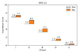
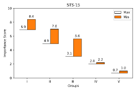
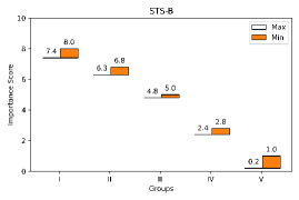
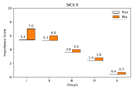
Figure 4: The importance score of five groups of features on STS benchmarks.

Appendix C Proof of Theorem 2

Before we start to prove the theorem, we provide some definitions that will be useful for further derivation:

Definition 1.

For a random variable $X$ with mean $\mu$, the moment generating function is

$$M_{X-\mu}(\lambda)=\mathbb{E}\exp(\lambda(X-\mathbb{E}X))$$ (15)

the cumulant-generating function is

$$\Gamma_{X-\mu}(\lambda)=\log M_{X-\mu}(\lambda)$$ (16)

We denote $D(X_{\text{P}},X)$ and $D(X_{\text{V}},X)$ as $D_{a}$ and $D_{b}$, and rewrite $D(X_{\text{P}},X)$ and $D(X_{\text{V}},X)$ as follows:

$$D(\mathcal{N}(\mu,\Sigma)\|\mathcal{N}(\hat{\mu},\hat{\Sigma}))\\ =\frac{1}{2}[\log(\frac{|\Sigma|}{|\epsilon I|})+\operatorname{tr}\left(\epsilon I\Sigma^{-1}\right)-k]$$ (17)

$$D(\mathcal{N}(\mu,\Sigma)\|\mathcal{N}(\hat{v},\epsilon I))\\ =\frac{1}{2}[\log(\frac{|\Sigma|}{|\hat{\Sigma}|})+\operatorname{tr}\left(\Sigma\hat{\Sigma}^{-1}\right)-k\\ +(\mu-\hat{\mu})^{\top}\hat{\Sigma}^{-1}(\mu-\hat{\mu})]$$ (18)

Proof 2.

As defined in the main paper, we have $D_{a}=D(\mathcal{N}(\mu,\Sigma)\|\mathcal{N}(\hat{\mu},\hat{\Sigma}))=\frac{1}{2}[\log(\frac{|\Sigma|}{|\epsilon I|})+\operatorname{tr}\left(\epsilon I\Sigma^{-1}\right)-p]$ and $D_{b}=D(\mathcal{N}(\mu,\Sigma)\|\mathcal{N}(\hat{v},\epsilon I))=\frac{1}{2}[\log(\frac{|\Sigma|}{|\hat{\Sigma}|})+\operatorname{tr}\left(\Sigma\hat{\Sigma}^{-1}\right)-p+(\mu-\hat{\mu})^{\top}\hat{\Sigma}^{-1}(\mu-\hat{\mu})]$. As illustrated in the methodology of Sen2Pro, we have the following derivation:

$$|\Sigma^{-1}|=\prod_{i=1}^{n}\frac{1}{\Sigma_{ii}}$$ (19)

$$|\Sigma|=\prod_{i=1}^{n}\Sigma_{ii}$$ (20)

Then we focus on the term:

$$D_{a} =D(\mathcal{N}(\mu,\Sigma)\|\mathcal{N}(\hat{\mu},\hat{\Sigma}))$$ (21)

$$=\frac{1}{2}[\log(\frac{|\Sigma|}{|\epsilon I|})+\operatorname{tr}\left(\epsilon I\Sigma^{-1}\right)-p]$$

$$\approx\frac{1}{2}[\log(\frac{|\Sigma|}{|\epsilon I|})-p]$$

since $\epsilon$ is an extremely small number. Besides, we also make derivation on $D_{b}$:

$$D_{a} =D(\mathcal{N}(\mu,\Sigma)\|\mathcal{N}(\hat{\mu},\hat{\Sigma}))$$ (22)

$$=\frac{1}{2}[\log(\frac{|\Sigma|}{|\hat{\Sigma}|})+\operatorname{tr}\left(\Sigma\hat{\Sigma}^{-1}\right)-p$$

$$+(\mu-\hat{\mu})^{\top}\hat{\Sigma}^{-1}(\mu-\hat{\mu})]$$

$$=\frac{1}{2}[\log(\frac{|\Sigma|}{|\hat{\Sigma}|})+(\mu-\hat{\mu})^{\top}\hat{\Sigma}^{-1}(\mu-\hat{\mu})]$$

To better analyze the $(\mu-\hat{\mu})^{\top}\hat{\Sigma}^{-1}(\mu-\hat{\mu})$ term of $D_{a}$, we present the following lemma:

Lemma 2.

For $X\sim N\left(\mu,\sigma^{2}\right)$, where $X$ is a single Gaussian variable,

$$\Gamma_{X-\mu}(\lambda)=\frac{\lambda^{2}\sigma^{2}}{2},\quad\quad\Gamma_{X-\mu}^{*}(\epsilon)=\frac{\epsilon^{2}}{2\sigma^{2}}.$$

For $X_{1},\ldots,X_{n}\sim N\left(\mu,\sigma^{2}\right)$, it’s easy to check that the bound is tight:

$$\lim_{n\rightarrow\infty}\frac{1}{n}\ln P\left(\bar{X}_{n}-\mu\geq\epsilon\right)=-\frac{\epsilon^{2}}{2\sigma^{2}}.$$

Therefore, we can represent $|\mu-\hat{\mu}|_{2}$ as $O(\epsilon)$ and we have the following:

$$(\mu-\hat{\mu})^{\top}\hat{\Sigma}^{-1}(\mu-\hat{\mu})$$ (23)

$$=D(\mathcal{N}(\mu,\Sigma)\|\mathcal{N}(\hat{\mu},\hat{\Sigma}))$$

$$=O(\epsilon^{2})$$

Naturally, we drop all $O(\epsilon^{2})$ term and formulate $D_{a}$ as follows:

$$D_{a}=\frac{1}{2}[\log(\frac{|\Sigma|}{|\hat{\Sigma}|})+\operatorname{tr}\left(\Sigma\hat{\Sigma}^{-1}\right)-p]$$ (24)

$$=\frac{1}{2}[\log(\frac{|\Sigma|}{|\hat{\Sigma}|})]$$ (25)

Then we insert the condition to the equality $D_{a}<D_{b}$, and we can complete the proof.

Appendix D Comparisons between individual estimation and unified estimation

This section conducts comparisons between individual estimation and unified estimation.

• Concretely, individual estimation refers to estimate $\mu^{m},\hat{\Sigma}^{m}$ and $\mu^{d},\hat{\Sigma}^{d}$ based on $\mathcal{S}^{m}$ and $\mathcal{S}^{d}$, respectively. Then we use $\frac{\mu^{m}+\mu^{d}}{2}$ and $\frac{\hat{\Sigma}^{m}+\hat{\Sigma}^{d}}{2}$ for sentence representation.

• Correspondingly, unified estimation refers to estimate $\mu^{u},\hat{\Sigma}^{u}$ based on $\mathcal{S}^{m}\cap\mathcal{S}^{d}$. Then use $\mu^{u},\hat{\Sigma}^{u}$ for sentence representation.

The experimental settings follow the Sec 4, and the results are shown in Table 10. We can observe that unified estimation under-performs individual estimation. Thus, we choose to estimate uncertainty in an individual way.

Model	STS-12	STS-13	STS-14	STS-15	STS-16	STS-B	SICK-R	Average
BERT-base	57.84	61.95	62.48	70.95	69.81	59.04	63.75	63.69
BERT-base-$G_{m+d}$	59.40	63.03	64.18	71.97	70.73	62.59	64.69	65.23 (+1.54)
BERT-base-$G_{u}$	58.86	62.66	63.77	71.48	70.56	61.89	64.28	64.79 (+1.02)

Table 10: BERT-base-$G_{m+d}$ and BERT-base-$G_{u}$ represent Sen2Pro with individual and unified estimation, respectively.

Appendix E Relation between model uncertainty and feature importance

This section serves as a complementary material for demonstrating the relation between the model uncertainty and feature importance, and the results on the STS task are illustrated in the Figure LABEL:a LABEL:b 4.

Appendix F Relation between model uncertainty and performance improvements

Figure 5: The relation between fluctuation rate ($Q$) and improvement score ($I$) on STS benchmarks.

This section serves as a complementary material for demonstrating the relation between the model uncertainty and performance improvements, and the results on the STS task are illustrated in the Figures 5.

Appendix G Influence of the Sampling Number

This section examines the effect of the sampling number $n_{1}$ in the model uncertainty and the sampling number $n_{2}$. To examine the effect of $n_{1}$, an experiment is run, where $n_{1}$ varies and $n_{2}$ is set $30$. The results of the STS and text classification task are illustrated in Figure 6. From Figure 6, we select $n_{1}=50$ and $n_{1}=15$ for the STS and text classification task, respectively, since smaller $n_{1}$ result in imprecise sentence representation and larger $n_{1}$ brings significant computational burden with little improvements. To examine the effect of the sampling number $n_{2}$, we change $n_{2}$ and keep the optimal $n_{1}$, and show the results in Figure 7. Overall, when $n_{2}$ is greater than 30, Sen2Pro achieves a stable performance.

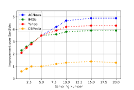
Figure 6: Results as the sampling number $n_{1}$ changes with ‘BERT-base-G’. The text classification task uses the ‘10-shot’ setting.

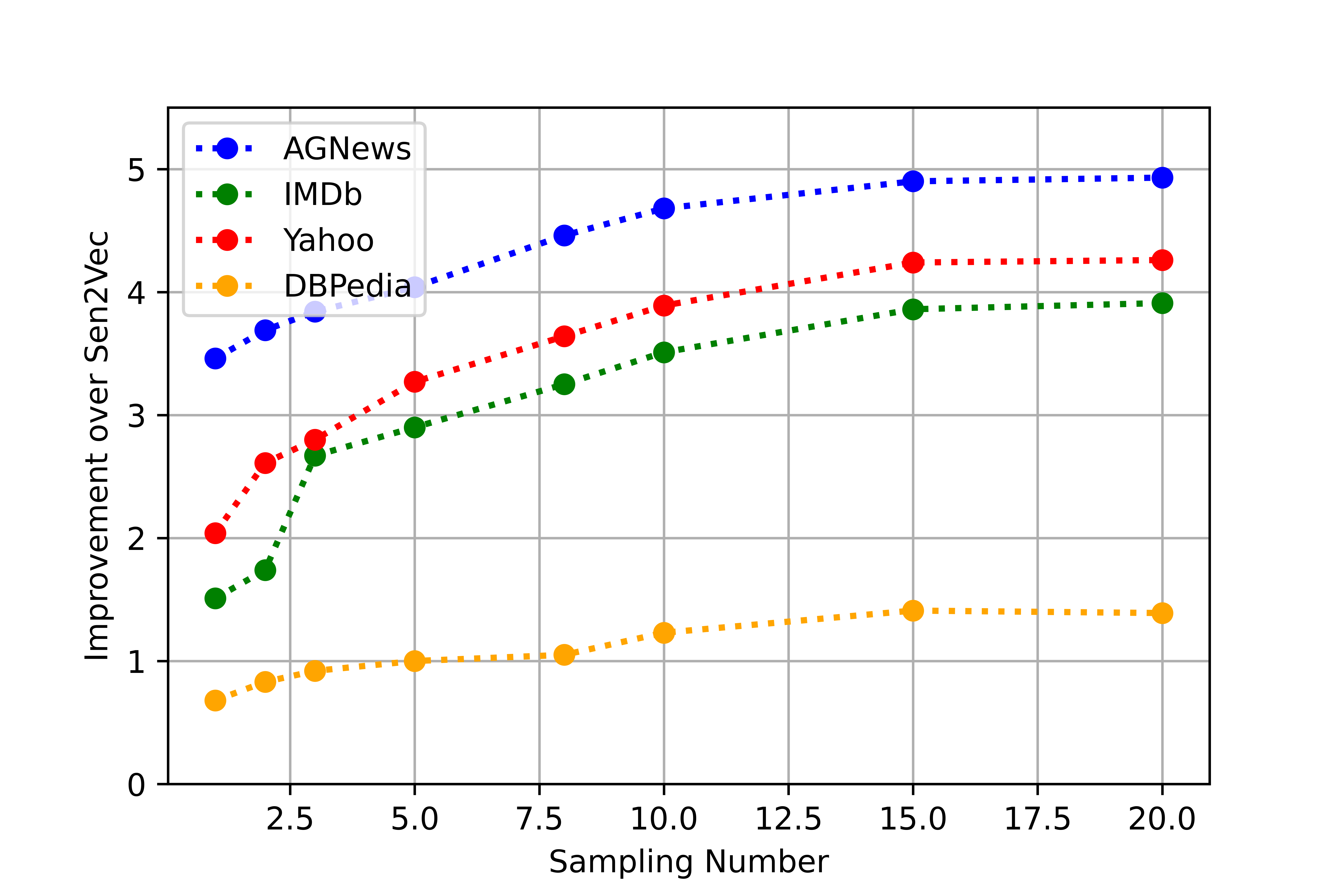
Figure 7: Results as sampling number $n_{2}$ changes with ‘BERT-base-G’. The text classification task uses the ‘10-shot’ setting.

Appendix H Results of Segment-level Evaluation of Neural Machine Translation

In the main paper, we make the evaluations on the system-level NMT. Here, we present the results of segment-level Evaluation of Neural Machine Translation. The experimental settings are kept the same as the ones in our main paper. The results are listed in Table 11. As the results demonstrate, Sen2Pro outperforms Sen2Vec and achieves comparable performances to BERTScore.

Metric	cs-en	de-en	fi-en	lv-en	ru-en	tr-en	zh-en	Avg
BLEU	23.3	41.5	28.5	15.4	22.8	14.5	17.8	21.2
ITER	19.8	39.6	23.5	12.8	13.9	2.9	14.4	18.1
RUSE	34.7	49.8	36.8	27.3	31.1	25.9	21.8	32.5
Sen2Vec	33.8	48.6	35.9	26.0	29.0	22.4	21.0	31.0
BERTScore	36.5	51.4	37.2	26.8	31.7	27.2	22.9	33.4
Sen2Pro	38.7	54.1	38.9	28.3	34.5	28.0	24.8	35.3

Table 11: Pearson correlations with segment-level machine translation evaluation on WMT17.

References

- Abdar et al. (2021) Moloud Abdar, Farhad Pourpanah, Sadiq Hussain, Dana Rezazadegan, Li Liu, Mohammad Ghavamzadeh, Paul Fieguth, Xiaochun Cao, Abbas Khosravi, U Rajendra Acharya, et al. 2021. A review of uncertainty quantification in deep learning: Techniques, applications and challenges. Information Fusion, 76:243–297.
- Agirre et al. (2015) Eneko Agirre, Carmen Banea, Claire Cardie, Daniel Cer, Mona Diab, Aitor Gonzalez-Agirre, Weiwei Guo, Inigo Lopez-Gazpio, Montse Maritxalar, Rada Mihalcea, et al. 2015. Semeval-2015 task 2: Semantic textual similarity, english, spanish and pilot on interpretability. In Proceedings of the 9th international workshop on semantic evaluation (SemEval 2015), pages 252–263.
- Agirre et al. (2014) Eneko Agirre, Carmen Banea, Claire Cardie, Daniel Cer, Mona Diab, Aitor Gonzalez-Agirre, Weiwei Guo, Rada Mihalcea, German Rigau, and Janyce Wiebe. 2014. Semeval-2014 task 10: Multilingual semantic textual similarity. In Proceedings of the 8th international workshop on semantic evaluation (SemEval 2014), pages 81–91.
- Agirre et al. (2016) Eneko Agirre, Carmen Banea, Daniel Cer, Mona Diab, Aitor Gonzalez Agirre, Rada Mihalcea, German Rigau Claramunt, and Janyce Wiebe. 2016. Semeval-2016 task 1: Semantic textual similarity, monolingual and cross-lingual evaluation. In SemEval-2016. 10th International Workshop on Semantic Evaluation; 2016 Jun 16-17; San Diego, CA. Stroudsburg (PA): ACL; 2016. p. 497-511. ACL (Association for Computational Linguistics).
- Agirre et al. (2012) Eneko Agirre, Daniel Cer, Mona Diab, and Aitor Gonzalez-Agirre. 2012. Semeval-2012 task 6: A pilot on semantic textual similarity. In * SEM 2012: The First Joint Conference on Lexical and Computational Semantics–Volume 1: Proceedings of the main conference and the shared task, and Volume 2: Proceedings of the Sixth International Workshop on Semantic Evaluation (SemEval 2012), pages 385–393.
- Agirre et al. (2013) Eneko Agirre, Daniel Cer, Mona Diab, Aitor Gonzalez-Agirre, and Weiwei Guo. 2013. * sem 2013 shared task: Semantic textual similarity. In Second joint conference on lexical and computational semantics (* SEM), volume 1: proceedings of the Main conference and the shared task: semantic textual similarity, pages 32–43.
- Bamler and Mandt (2017) Robert Bamler and Stephan Mandt. 2017. Dynamic word embeddings. In International conference on Machine learning, pages 380–389. PMLR.
- Bengio et al. (2003) Yoshua Bengio, Réjean Ducharme, Pascal Vincent, and Christian Janvin. 2003. A neural probabilistic language model. The journal of machine learning research, 3:1137–1155.
- Bickel and Levina (2008) Peter J Bickel and Elizaveta Levina. 2008. Regularized estimation of large covariance matrices. The Annals of Statistics, 36(1):199–227.
- Bien et al. (2016) Jacob Bien, Florentina Bunea, and Luo Xiao. 2016. Convex banding of the covariance matrix. Journal of the American Statistical Association, 111(514):834–845.
- Bojar et al. (2017) Ondřej Bojar, Jindřich Helcl, Tom Kocmi, Jindřich Libovickỳ, and Tomáš Musil. 2017. Results of the wmt17 neural mt training task. In Proceedings of the second conference on machine translation, pages 525–533.
- Camacho-Collados and Pilehvar (2018) Jose Camacho-Collados and Mohammad Taher Pilehvar. 2018. From word to sense embeddings: A survey on vector representations of meaning. Journal of Artificial Intelligence Research, 63:743–788.
- Chang et al. (2008) Ming-Wei Chang, Lev-Arie Ratinov, Dan Roth, and Vivek Srikumar. 2008. Importance of semantic representation: Dataless classification. In Aaai, volume 2, pages 830–835.
- Chen et al. (2016) Xi Chen, Yan Duan, Rein Houthooft, John Schulman, Ilya Sutskever, and Pieter Abbeel. 2016. Infogan: Interpretable representation learning by information maximizing generative adversarial nets. In Proceedings of the 30th International Conference on Neural Information Processing Systems, pages 2180–2188.
- Clark et al. (2019) Kevin Clark, Minh-Thang Luong, Quoc V Le, and Christopher D Manning. 2019. Electra: Pre-training text encoders as discriminators rather than generators. In International Conference on Learning Representations.
- Cover (1999) Thomas M Cover. 1999. Elements of information theory. John Wiley & Sons.
- Denkowski and Lavie (2014) Michael Denkowski and Alon Lavie. 2014. Meteor universal: Language specific translation evaluation for any target language. In Proceedings of the ninth workshop on statistical machine translation, pages 376–380.
- Devlin et al. (2019) Jacob Devlin, Ming-Wei Chang, Kenton Lee, and Kristina Toutanova. 2019. Bert: Pre-training of deep bidirectional transformers for language understanding. In Proceedings of the 2019 Conference of the North American Chapter of the Association for Computational Linguistics: Human Language Technologies, Volume 1 (Long and Short Papers), pages 4171–4186.
- Dinan et al. (2020) Emily Dinan, Varvara Logacheva, Valentin Malykh, Alexander Miller, Kurt Shuster, Jack Urbanek, Douwe Kiela, Arthur Szlam, Iulian Serban, Ryan Lowe, et al. 2020. The second conversational intelligence challenge (convai2). In The NeurIPS’18 Competition, pages 187–208. Springer.
- Forgues et al. (2014) Gabriel Forgues, Joelle Pineau, Jean-Marie Larchevêque, and Réal Tremblay. 2014. Bootstrapping dialog systems with word embeddings. In Nips, modern machine learning and natural language processing workshop, volume 2.
- Gal and Ghahramani (2016) Yarin Gal and Zoubin Ghahramani. 2016. Dropout as a bayesian approximation: Representing model uncertainty in deep learning. In international conference on machine learning, pages 1050–1059. PMLR.
- Gao et al. (2021) Tianyu Gao, Xingcheng Yao, and Danqi Chen. 2021. Simcse: Simple contrastive learning of sentence embeddings. arXiv preprint arXiv:2104.08821.
- Gao et al. (2019) Weihao Gao, Yu-Han Liu, Chong Wang, and Sewoong Oh. 2019. Rate distortion for model compression: From theory to practice. In International Conference on Machine Learning, pages 2102–2111. PMLR.
- Grohs et al. (2021) Philipp Grohs, Andreas Klotz, and Felix Voigtlaender. 2021. Phase transitions in rate distortion theory and deep learning. Foundations of Computational Mathematics, pages 1–64.
- He et al. (2020) Pengcheng He, Xiaodong Liu, Jianfeng Gao, and Weizhu Chen. 2020. Deberta: Decoding-enhanced bert with disentangled attention. In International Conference on Learning Representations.
- Hill et al. (2016) Felix Hill, Kyunghyun Cho, and Anna Korhonen. 2016. Learning distributed representations of sentences from unlabelled data. In Proceedings of the 2016 Conference of the North American Chapter of the Association for Computational Linguistics: Human Language Technologies, pages 1367–1377.
- Howard and Ruder (2018) Jeremy Howard and Sebastian Ruder. 2018. Universal language model fine-tuning for text classification. In Proceedings of the 56th Annual Meeting of the Association for Computational Linguistics (Volume 1: Long Papers), pages 328–339.
- Huang et al. (2021) Junjie Huang, Duyu Tang, Wanjun Zhong, Shuai Lu, Linjun Shou, Ming Gong, Daxin Jiang, and Nan Duan. 2021. Whiteningbert: An easy unsupervised sentence embedding approach. arXiv preprint arXiv:2104.01767.
- Hüllermeier and Waegeman (2021) Eyke Hüllermeier and Willem Waegeman. 2021. Aleatoric and epistemic uncertainty in machine learning: An introduction to concepts and methods. Machine Learning, 110(3):457–506.
- Kendall and Gal (2017) Alex Kendall and Yarin Gal. 2017. What uncertainties do we need in bayesian deep learning for computer vision? Advances in neural information processing systems, 30.
- Kiros et al. (2015) Ryan Kiros, Yukun Zhu, Russ R Salakhutdinov, Richard Zemel, Raquel Urtasun, Antonio Torralba, and Sanja Fidler. 2015. Skip-thought vectors. In Advances in neural information processing systems, pages 3294–3302.
- Lakshminarayanan et al. (2017) Balaji Lakshminarayanan, Alexander Pritzel, and Charles Blundell. 2017. Simple and scalable predictive uncertainty estimation using deep ensembles. Advances in neural information processing systems, 30.
- Leusch et al. (2006) Gregor Leusch, Nicola Ueffing, and Hermann Ney. 2006. Cder: Efficient mt evaluation using block movements. In 11th Conference of the European Chapter of the Association for Computational Linguistics.
- Li and Chen (2019) Qing Li and Yang Chen. 2019. Rate distortion via deep learning. IEEE Transactions on Communications, 68(1):456–465.
- Lin (2004) Chin-Yew Lin. 2004. Rouge: A package for automatic evaluation of summaries. In Text summarization branches out, pages 74–81.
- Liu et al. (2019) Yinhan Liu, Myle Ott, Naman Goyal, Jingfei Du, Mandar Joshi, Danqi Chen, Omer Levy, Mike Lewis, Luke Zettlemoyer, and Veselin Stoyanov. 2019. Roberta: A robustly optimized bert pretraining approach.
- Lowe et al. (2017) Ryan Lowe, Michael Noseworthy, Iulian Vlad Serban, Nicolas Angelard-Gontier, Yoshua Bengio, and Joelle Pineau. 2017. Towards an automatic turing test: Learning to evaluate dialogue responses. In Proceedings of the 55th Annual Meeting of the Association for Computational Linguistics (Volume 1: Long Papers), pages 1116–1126.
- Ma et al. (2017) Qingsong Ma, Yvette Graham, Shugen Wang, and Qun Liu. 2017. Blend: a novel combined mt metric based on direct assessment—casict-dcu submission to wmt17 metrics task. In Proceedings of the second conference on machine translation, pages 598–603.
- Maas et al. (2011) Andrew Maas, Raymond E Daly, Peter T Pham, Dan Huang, Andrew Y Ng, and Christopher Potts. 2011. Learning word vectors for sentiment analysis. In Proceedings of the 49th annual meeting of the association for computational linguistics: Human language technologies, pages 142–150.
- Maddox et al. (2019) Wesley J Maddox, Pavel Izmailov, Timur Garipov, Dmitry P Vetrov, and Andrew Gordon Wilson. 2019. A simple baseline for bayesian uncertainty in deep learning. Advances in Neural Information Processing Systems, 32.
- Meng et al. (2021) Yu Meng, Chenyan Xiong, Payal Bajaj, Saurabh Tiwary, Paul Bennett, Jiawei Han, and Xia Song. 2021. Coco-lm: Correcting and contrasting text sequences for language model pretraining.
- Mikolov et al. (2013) Tomas Mikolov, Ilya Sutskever, Kai Chen, Greg S Corrado, and Jeff Dean. 2013. Distributed representations of words and phrases and their compositionality. In Advances in neural information processing systems, pages 3111–3119.
- Ovadia et al. (2019) Yaniv Ovadia, Emily Fertig, Jie Ren, Zachary Nado, David Sculley, Sebastian Nowozin, Joshua Dillon, Balaji Lakshminarayanan, and Jasper Snoek. 2019. Can you trust your model’s uncertainty? evaluating predictive uncertainty under dataset shift. Advances in neural information processing systems, 32.
- Papineni et al. (2002) Kishore Papineni, Salim Roukos, Todd Ward, and Wei-Jing Zhu. 2002. Bleu: a method for automatic evaluation of machine translation. In Proceedings of the 40th annual meeting of the Association for Computational Linguistics, pages 311–318.
- Pennington et al. (2014) Jeffrey Pennington, Richard Socher, and Christopher D Manning. 2014. Glove: Global vectors for word representation. In Proceedings of the 2014 conference on empirical methods in natural language processing (EMNLP), pages 1532–1543.
- Peters et al. (2018) Matthew E. Peters, Mark Neumann, Mohit Iyyer, Matt Gardner, Christopher Clark, Kenton Lee, and Luke Zettlemoyer. 2018. Deep contextualized word representations. In Proceedings of the 2018 Conference of the North American Chapter of the Association for Computational Linguistics: Human Language Technologies, Volume 1 (Long Papers), pages 2227–2237, New Orleans, Louisiana. Association for Computational Linguistics.
- Radford et al. (2019) Alec Radford, Jeffrey Wu, Rewon Child, David Luan, Dario Amodei, Ilya Sutskever, et al. 2019. Language models are unsupervised multitask learners. OpenAI blog, 1(8):9.
- Raffel et al. (2020) Colin Raffel, Noam Shazeer, Adam Roberts, Katherine Lee, Sharan Narang, Michael Matena, Yanqi Zhou, Wei Li, and Peter J Liu. 2020. Exploring the limits of transfer learning with a unified text-to-text transformer. Journal of Machine Learning Research, 21(140):1–67.
- Rashkin et al. (2019) Hannah Rashkin, Eric Michael Smith, Margaret Li, and Y-Lan Boureau. 2019. Towards empathetic open-domain conversation models: A new benchmark and dataset. In Proceedings of the 57th Annual Meeting of the Association for Computational Linguistics, pages 5370–5381.
- Reimers and Gurevych (2019) Nils Reimers and Iryna Gurevych. 2019. Sentence-bert: Sentence embeddings using siamese bert-networks. In Proceedings of the 2019 Conference on Empirical Methods in Natural Language Processing and the 9th International Joint Conference on Natural Language Processing (EMNLP-IJCNLP), pages 3982–3992.
- Rus and Lintean (2012) Vasile Rus and Mihai Lintean. 2012. An optimal assessment of natural language student input using word-to-word similarity metrics. In International Conference on Intelligent Tutoring Systems, pages 675–676. Springer.
- Shen et al. (2022a) Lingfeng Shen, Haiyun Jiang, Lemao Liu, and Shuming Shi. 2022a. Revisiting the evaluation metrics of paraphrase generation. arXiv preprint arXiv:2202.08479.
- Shen et al. (2022b) Lingfeng Shen, Lemao Liu, Haiyun Jiang, and Shuming Shi. 2022b. On the evaluation metrics for paraphrase generation. In Proceedings of the 2022 Conference on Empirical Methods in Natural Language Processing, pages 3178–3190.
- Su et al. (2021) Jianlin Su, Jiarun Cao, Weijie Liu, and Yangyiwen Ou. 2021. Whitening sentence representations for better semantics and faster retrieval. arXiv preprint arXiv:2103.15316.
- Tschannen et al. (2019) Michael Tschannen, Josip Djolonga, Paul K Rubenstein, Sylvain Gelly, and Mario Lucic. 2019. On mutual information maximization for representation learning. In International Conference on Learning Representations.
- Vilnis and McCallum (2015) Luke Vilnis and Andrew McCallum. 2015. Word representations via gaussian embedding. In ICLR.
- Wang et al. (2022) Bin Wang, C-c Kuo, and Haizhou Li. 2022. Just rank: Rethinking evaluation with word and sentence similarities. In Proceedings of the 60th Annual Meeting of the Association for Computational Linguistics (Volume 1: Long Papers), pages 6060–6077.
- Wang et al. (2021) Dong Wang, Ning Ding, Piji Li, and Haitao Zheng. 2021. Cline: Contrastive learning with semantic negative examples for natural language understanding. In Proceedings of the 59th Annual Meeting of the Association for Computational Linguistics and the 11th International Joint Conference on Natural Language Processing (Volume 1: Long Papers), pages 2332–2342.
- Wieting et al. (2015a) John Wieting, Mohit Bansal, Kevin Gimpel, and Karen Livescu. 2015a. From paraphrase database to compositional paraphrase model and back. Transactions of the Association for Computational Linguistics, 3:345–358.
- Wieting et al. (2015b) John Wieting, Mohit Bansal, Kevin Gimpel, and Karen Livescu. 2015b. Towards universal paraphrastic sentence embeddings. arXiv preprint arXiv:1511.08198.
- Xiao and Wu (2012) Han Xiao and Wei Biao Wu. 2012. Covariance matrix estimation for stationary time series. The Annals of Statistics, 40(1):466–493.
- Yan et al. (2021) Yuanmeng Yan, Rumei Li, Sirui Wang, Fuzheng Zhang, Wei Wu, and Weiran Xu. 2021. Consert: A contrastive framework for self-supervised sentence representation transfer. arXiv preprint arXiv:2105.11741.
- Zhang et al. (2019) Tianyi Zhang, Varsha Kishore, Felix Wu, Kilian Q Weinberger, and Yoav Artzi. 2019. Bertscore: Evaluating text generation with bert. In International Conference on Learning Representations.
- Zhang et al. (2015) Xiang Zhang, Junbo Zhao, and Yann LeCun. 2015. Character-level convolutional networks for text classification. Advances in neural information processing systems, 28:649–657.
- Zhang et al. (2020) Yan Zhang, Ruidan He, Zuozhu Liu, Kwan Hui Lim, and Lidong Bing. 2020. An unsupervised sentence embedding method by mutual information maximization. In Proceedings of the 2020 Conference on Empirical Methods in Natural Language Processing (EMNLP), pages 1601–1610.
- Zhou et al. (2019) Chunting Zhou, Xuezhe Ma, Di Wang, and Graham Neubig. 2019. Density matching for bilingual word embedding. In Proceedings of the 2019 Conference of the North American Chapter of the Association for Computational Linguistics: Human Language Technologies, Volume 1 (Long and Short Papers), pages 1588–1598.
- Zhu and de Melo (2020) Xunjie Zhu and Gerard de Melo. 2020. Sentence analogies: Linguistic regularities in sentence embeddings. In Proceedings of the 28th International Conference on Computational Linguistics, pages 3389–3400.