On the Generalized Mean Densest Subgraph Problem: Complexity and Algorithms

Abstract

Dense subgraph discovery is an important problem in graph mining and network analysis with several applications. Two canonical problems here are to find a maxcore (subgraph of maximum min degree) and to find a densest subgraph (subgraph of maximum average degree). Both of these problems can be solved in polynomial time. Veldt, Benson, and Kleinberg [VBK21] introduced the generalized $p$-mean densest subgraph problem which captures the maxcore problem when $p=-\infty$ and the densest subgraph problem when $p=1$. They observed that the objective leads to a supermodular function when $p\geq 1$ and hence can be solved in polynomial time; for this case, they also developed a simple greedy peeling algorithm with a bounded approximation ratio. In this paper, we make several contributions. First, we prove that for any $p\in(-\frac{1}{8},0)\cup(0,\frac{1}{4})$ the problem is NP-Hard and for any $p\in(-3,0)\cup(0,1)$ the weighted version of the problem is NP-Hard, partly resolving a question left open in [VBK21]. Second, we describe two simple $1/2$-approximation algorithms for all $p<1$, and show that our analysis of these algorithms is tight. For $p>1$ we develop a fast near-linear time implementation of the greedy peeling algorithm from [VBK21]. This allows us to plug it into the iterative peeling algorithm that was shown to converge to an optimum solution [CQT22]. We demonstrate the efficacy of our algorithms by running extensive experiments on large graphs. Together, our results provide a comprehensive understanding of the complexity of the $p$-mean densest subgraph problem and lead to fast and provably good algorithms for the full range of $p$.

1 Introduction

Dense subgraph discovery is an essential tool in graph mining and network analysis. One can view the approach as finding clusters or communities in a graph where the edges between the nodes in the cluster are denser compared to those in the entire graph. There are a number applications of dense subgraph discovery in biological settings [HYH⁺05, FNBB06, LBG20], protein-protein interaction networks [BH03, SM03], web mining [GKT05, DGP07], social network analysis [KNT06], real-time story identification [AKS⁺14], and finance and fraud detection [DJD⁺09, ZZY⁺17, JZT⁺22].

Different density definitions are used and studied in the literature, motivated by the needs of applications and theoretical considerations (see [FRM19, GT15, LRJA10, TC21] for some surveys). Each density definition leads to a corresponding combinatorial optimization problem: given a graph $G$, find a subgraph of maximum density. Two of the most popular density measures in the literature are (i) the minimum degree of the subgraph and (ii) the average degree of the subgraph. These measures lead to the maxcore problem and densest subgraph problem (DSG); the goal is to find the subgraph with the maximum minimum degree and maximum average degree, respectively. They are both polynomial-time solvable and have been extensively studied. We briefly describe them before discussing a common generalization that is the focus of this paper.

A $k$-core of a graph is a maximal connected subgraph with all vertices of degree at least $k$. The largest value of $k$ for which $G$ contains a $k$-core is known as the degeneracy. We refer to the $k$-core obtaining this maximum as the maxcore. $k$-cores are a popular notion of density, commonly finding use in what is known as the $k$-core decomposition, a nested sequence of subgraphs that captures all $k$-cores. One nice feature of a $k$-core decomposition is that there is a simple linear-time peeling algorithm $\mathsf{Greedy}$ to compute it. We refer the reader to [MGPV20] for a survey on $k$-core decomposition and applications.

The densest subgraph problem (DSG), where the goal is to find a subgraph of maximum average degree, is a classical problem in combinatorial optimzation that is polynomial time solvable [Cha00, GGT89] via network flow techniques among others. It is widely studied in graph mining. Even though DSG can be solved exactly, the algorithms are slow and this has spurred a study of approximation algorithms for DSG [Cha00, BGM14, DCS17, BSW19, BGP⁺20, CQT22, HQC22]. Amongst these approximation algorithms is the algorithm $\mathsf{Greedy}$ introduced by Asahiro et al. [AITT00] to solve DSG and shown to be a $\frac{1}{2}$-approximation by Charikar [Cha00]. Note that the peeling order is the same as the one for computing the optimum $k$-core decomposition; it is only in the second step where one checks all suffixes that the specific density measure for DSG is used. Charikar’s analysis has spurred the development and analysis of a variety of peeling algorithms for several variants of DSG in both graphs and hypergraphs [AC09, Tso14, Tso15, HWC17, KM18, VBK21].

Veldt, Benson and Kleinberg [VBK21] introduced the generalized mean densest subgraph problem. It is a common generalization of the two problems we described in the preceding paragraphs and is the focus of this paper. Given a real parameter $p\in\mathbb{R}\cup\{-\infty,\infty\}$ and an undirected graph $G=(V,E)$, the density of a subgraph $G[S]$ induced by a set $S\subseteq V$ is defined as:

$$M_{p}(S):=\left(\frac{1}{\left|S\right|}\sum_{v\in S}d_{S}(v)^{p}\right)^{1/p}$$

where $d_{S}(v)$ is the degree of the vertex $v$ in $G[S]$. To make the dependence on $p$ more explicit, we refer to this problem also as the $p$-mean densest subgraph problem ($p$-mean DSG). Note that $M_{-\infty}(S)=\min_{v\in S}d_{S}(v)$ is the minimum degree in $G[S]$, $M_{\infty}(S)=\max_{v\in S}d_{S}(v)$ is the maximum degree, $M_{1}(S)=2|E(S)|/|S|$ is twice the average degree of $G[S]$, and $M_{0}(S)=(\prod_{v\in S}d_{S}(v))^{1/\left|S\right|}$, which can be transformed to $\frac{1}{\left|S\right|}\sum_{v\in S}\log d_{S}(v)$ by taking the logarithm of the objective. Thus, $p$-mean DSG for different values of $p$ captures two of the most well-studied problems in dense subgraph discovery. As $p$ varies from $-\infty$ to $\infty$, $M_{p}(S)$ prioritizes the smallest degree in $S$ to the largest degree in $S$ and provides a smooth way to generate subgraphs with different density properties.

Veldt et al. made several contributions to $p$-mean DSG. They observed that $1$-mean DSG is equivalent to DSG and that $-\infty$-mean DSG is equivalent to finding the maxcore. For $p\geq 1$, they observe the set function $f_{p}:2^{V}\rightarrow\mathbb{R}_{+}$ where $f_{p}(S):=\sum_{v\in S}d_{S}(v)^{p}$ is a supermodular function. This implies that one can solve $p$-mean DSG in polynomial time for all $p>1$ via a standard reduction to submodular set function minimization, a classical result in combinatorial optimization [Sch03]. Note that the function $f_{p}(S)$ is not supermodular when $p<1$, which partially stems from the fact that $x^{p}$ is not convex in $x$ when $p<1$. Motivated by the fact that exact algorithms are very slow in practice, they describe a greedy peeling algorithm $\mathsf{Greedy\text{-}}p$ that runs in $O(mn)$ time and is a $\left(\frac{1}{p+1}\right)^{1/p}$-approximation (here $m$ and $n$ are the number of edges and nodes of the graph). Note that the peeling order of $\mathsf{Greedy\text{-}}p$ is not the same as that of $\mathsf{Greedy}$ and depends on $p$. They supplement this work with experiments, showing that $\mathsf{Greedy\text{-}}p$ returns solutions with desirable characteristics for values of $p$ in the range $[1,2]$.

Motivation for this work.

In this paper we are interested in algorithms for $p$-mean DSG that are theoretically and empirically sound, and its complexity status for $p<1$ which was left open in [VBK21]. It is intriguing that $p=-\infty$ and $p\geq 1$ are both polynomial-time solvable while the status of $p\in(-\infty,1)$ is non-trivial to understand. We focus on the case of $p\in(-\infty,0)\cup(0,1)$ as the objective for $p=0$ is significantly different. Second, we are interested in developing fast approximation algorithms for $p$-mean DSG when $p>1$ and when $p<1$. The $O(mn)$-time algorithm in [VBK21] is slow for large graphs. Moreover, for $p>1$, it is of substantial interest to find algorithms that provably converge to an optimum solution rather than provide a constant factor approximation (since the problem is efficiently solvable). Such algorithms have been of much interest for the classical DSG problem [BGM14, DCS17, BSW19, BGP⁺20, CQT22, HQC22].

This paper is also motivated by a few recent works. One of them is a paper of Chekuri, Quanrud, and Torres [CQT22] that introduced a framework under which one can understand some of the results of [VBK21]. In [CQT22], they observe that many notions of density in the literature are of the form $\frac{f(S)}{\left|S\right|}$ where $f:2^{V}\to\mathbb{R}$ is a supermodular function. They refer to this general problem as the densest supermodular subset problem (DSS). DSS captures $p$-mean DSG for $p\geq 1$. One can see this by noting that for $p\geq 1$, finding $\operatorname*{arg\,max}_{S}M_{p}(S)$ is equivalent to finding $\operatorname*{arg\,max}_{S}M_{p}(S)^{p}$. Thus, for $p\geq 1$, $p$-mean DSG is equivalent to $\max_{S}\frac{f_{p}(S)}{\left|S\right|}$. [CQT22] describes a simple peeling algorithm for DSS whose approximation guarantee depends on the supermodular function $f$; they refer to this as $\mathsf{SuperGreedy}$. In particular, $\mathsf{Greedy\text{-}}p$ is the same as $\mathsf{SuperGreedy}$ when specialized to $f_{p}$, and the analysis in [CQT22] recovers the one in [VBK21] for $p$-mean DSG. It is also shown in [CQT22] that an iterated peeling algorithm, called $\mathsf{SuperGreedy}\nolinebreak[4]\raisebox{1.72218pt}{{{++}}}$, converges to an optimum solution for DSS (thus, for any supermodular function). $\mathsf{SuperGreedy}\nolinebreak[4]\raisebox{1.72218pt}{{{++}}}$ is motivated by and generalizes the iterated greedy algorithm $\mathsf{Greedy}\nolinebreak[4]\raisebox{1.72218pt}{{{++}}}$ that was suggested by Boob et al. [BGP⁺20] for DSG. When one specializes $\mathsf{SuperGreedy}\nolinebreak[4]\raisebox{1.72218pt}{{{++}}}$ to $p$-mean DSG, the algorithm converges to a $(1-\epsilon)$-approximation in $O(\frac{\Delta_{p}\log n}{\lambda^{*}\epsilon^{2}})$ iterations where $\Delta_{p}=\max_{v\in V}f_{p}(V)-f_{p}(V-v)$ and $\lambda^{*}$ is the optimal density. A naive implementation yields a per-iteration running time of $O(mn)$. Another iterative algorithm that converges to an optimum solution for DSS is described in the work of Harb et al. [HQC22] and is based on the well-known Frank-Wolfe method applied to DSS; this is inspired by the algorithm of Danisch et al. [DCS17] for DSG. When one specializes this algorithm to $p$-mean DSG, a naive implementation yields a per-iteration running time of $O(m+n\log n)$. Since $p$-mean DSG for $p\geq 1$ is a special case of DSS, these two iterative algorithms will also converge to an optimum solution for $p$-mean DSG.

1.1 Our Results

As remarked earlier, our goal is to understand the complexity of $p$-mean DSG and develop improved algorithms for all values of $p$. We make four contributions in this paper towards this goal and we outline them below with some discussion of each.

NP-Hardness of $p$-mean DSG for $p<1$.

We prove that $p$-mean DSG is NP-Hard for any fixed $p\in(-\frac{1}{8},0)\cup(0,\frac{1}{4})$ and $p$-mean DSG for weighted graphs is NP-Hard for any fixed $p\in(-3,0)\cup(0,1)$. The hardness reduction is technically involved, especially due to the non-linear objective function. Our proof involves numerical computation and we restrict our attention to the range $(-\frac{1}{8},0)\cup(0,\frac{1}{4})$ for the unweighted case and $(-3,0)\cup(0,1)$ for the weighted case to make the calculations and the proof transparent. We believe that our proof methodology extends to all $p\in(-\infty,0)\cup(0,1)$ and describe an outline to do so.

$\frac{1}{2}$-approximation algorithms for $p\in(-\infty,1)$.

Our NP-Hardness result for $p$-mean DSG motivates the search for approximation algorithms and heuristics when $p<1$. In [VBK21] the authors do some empirical evaluation using $\mathsf{Greedy\text{-}}p$ for $p\in(0,1)$ even though the corresponding function $f_{p}$ is not supermodular; no approximation guarantee is known for this algorithm. $\mathsf{Greedy\text{-}}p$ is only well-defined for $p>0$. We describe two different and simple $\frac{1}{2}$-approximation algorithms for $p$-mean DSG when $p\in(-\infty,1)$, one based on simple greedy peeling and the other based on an exact solution to DSG. These are the first algorithms with approximation guarantees for this regime of $p$. We also show that $\frac{1}{2}$ is tight for these algorithms. We describe another algorithm, based on iterative peeling, that interpolates between the preceding two algorithms. It is also guaranteed to be a $\frac{1}{2}$-approximation but allows us to generate several candidate solutions along the way in a natural fashion.

Fast and improved algorithms for $p>1$.

Greedy-$p$ from [VBK21] runs in $O(mn)$ time, which is slow for large high-degree graphs. We describe a near-linear time algorithm for $p$-mean DSG when $p>1$. This algorithm, $\mathsf{Lazy\text{-}Greedy\text{-}}p$, is effectively a faster implementation of $\mathsf{Greedy\text{-}}p$ that utilizes lazy updates to improve the running time to $\tilde{O}(\frac{pm}{\epsilon})$ while only losing a factor of $(1-\epsilon)$ in the approximation ratio compared to $\mathsf{Greedy\text{-}}p$. Another important motivation and utility for $\mathsf{Lazy\text{-}Greedy\text{-}}p$ is the following. Recall the preceding discussion that iterating the greedy peeling algorithm yields an algorithm that converges to the optimum solution [CQT22]. However, iterating the vanilla implementation of $\mathsf{Greedy\text{-}}p$ is too slow for large graphs. In contrast, the faster $\mathsf{Lazy\text{-}Greedy\text{-}}p$ allows us to run many iterations on large graphs and gives good results in a reasonable amount of time.

Experiments.

We empirically evaluate the efficacy of our algorithms and some variations on a collection of ten publicly available large real-world graphs. For $p>1$, we show that $\mathsf{Lazy\text{-}Greedy\text{-}}p$ returns solutions with densities close to that of $\mathsf{Greedy\text{-}}p$ while running typically at least $2$ to $4$ times as fast. We evaluate the performance of the two iterative algorithms that provably converge to an optimum solution and compare their performance. We find that our algorithm converges faster on all graphs and values of $p$ tested. For $p<1$, we empirically evaluate our two new approximation algorithms, and we compare against $\mathsf{Greedy\text{-}}p$ which was tested in [VBK21] as a heuristic. We compare the three algorithms both for their running time and solution quality and report our findings for different values of $p\in(0,1)$. One of our approximation algorithms significantly outperforms all algorithms tested in terms of running time while returning a subgraph with comparable solution quality.

Organization.

In an effort to highlight the algorithmic aspects of our work, we start by describing and analyzing $\mathsf{Lazy\text{-}Greedy\text{-}}p$ in Section 4 and presenting our two new approximation algorithms for $p<1$ in Section 5. We also discuss our heuristics for $p>1$ and $p<1$ based on iterative algorithms for $p$-mean DSG in Section 5. We then present our hardness result in Section 6. We conclude with experiments in Section 7. All proofs that are omitted from the main body of the paper are contained in the appendix.

2 Related work

DSG has been the impetus for a wide-ranging and extensive subfield of research. The problem is solvable in polynomial time via different methods, such as a reduction to maximum flow [Gol84, Law76, PQ82, GGT89], a reduction to submodular minimization, and via an exact LP relaxation [Cha00]. Running times of these algorithms are relatively slow and thus approximation algorithms have been considered. The theoretically fastest known approximations run in near-linear time, obtaining $(1-\epsilon)$-approximations in $\tilde{O}(m\cdot\operatorname{poly}(\frac{1}{\epsilon}))$ time [BGM14, BSW19, CQT22]. The fastest known running time is $\tilde{O}(\frac{m}{\epsilon})$ [CQT22]. These algorithms are relatively complex to implement and practitioners often prefer simpler approximation algorithms but with worse approximation ratios, such as $\mathsf{Greedy}$ [AITT00, Cha00] and $\mathsf{Greedy}\nolinebreak[4]\raisebox{1.72218pt}{{{++}}}$ [BGP⁺20, CQT22]. However, there has been recent work that showed that one can obtain near-optimal solutions using continuous optimization methods that are both simple and efficient on large real-world graphs [DCS17, HQC22].

We discuss some of the density definitions considered in the literature. Given a graph $G=(V,E)$ and a finite collection of pattern graphs $\mathcal{F}$, many densities take the form $\frac{f(S)}{\left|S\right|}$ where $f:2^{V}\to\mathbb{R}$ counts the number of occurrences of the patterns in $\mathcal{F}$ in the induced subgraph $G[S]$. This exact problem was considered in [Far08]. [Tso14] considered the special case where $\mathcal{F}$ is a single triangle graph and [Tso15] considered the special case where $\mathcal{F}$ is a single clique on $k$ vertices. One can also consider a version of DSG for hypergraphs, where the density is defined as $\frac{\left|E(S)\right|}{\left|S\right|}$ where $E(S)$ is the set of hyperedges with all vertices in $S$ [HWC17]. We can reduce the pattern graph problem to the hypergraph problem by introducing a hyperedge for each occurrence of the pattern in the input graph. Other density definitions look at modifying DSG by considering the density $\frac{\left|E(S)\right|}{g(\left|S\right|)}$ where $g$ is an arbitrary function of $\left|S\right|$ [KM18]. Given a parameter $\alpha$, another density considers $\frac{\left|E(S)\right|-\alpha\left|\delta(S)\right|}{\left|S\right|}$ [MK18], which has connections to modularity density maximization [LZW⁺08, SMT22]. The $p$-mean DSG objective $M_{p}$ is a class of densities that captures a wide-range of different objectives, including DSG when $p=1$ and the maxcore problem when $p=-\infty$ [VBK21]. Aside from the variation modifying the denominator of DSG from [KM18], all of the different densities mentioned above fall into the framework of DSS where we want to maximize $\frac{f(S)}{\left|S\right|}$ for a supermodular function $f$ [CQT22].

This field of research is vast and we cannot hope to do it justice here, so we point the reader to five separate tutorials/surveys on the topic and the references therein [FRM19, GT15, LRJA10, TC21, LMFB23].

3 Preliminaries

Fix a graph $G=(V,E)$. Let $d_{S}(v)$ denote the degree of $v$ in the induced subgraph $G[S]$. Let $N(v)$ denote the neighborhood of $v$ in $G$. For any $p\in\mathbb{R}\cup\{-\infty,\infty\}$, and any $S\subseteq V$, we define $f_{p}(S):=\sum_{v\in S}d_{S}(v)^{p}$, $\rho_{p}(S):=\frac{f_{p}(S)}{\left|S\right|}$ and $M_{p}(S):=\rho_{p}(S)^{1/p}$. We let $S_{p}^{*}(G)$ denote $\operatorname*{arg\,max}_{S\subseteq V}M_{p}(S)$ and let $M_{p}^{*}(G):=M_{p}(S_{p}^{*})$. Note we use $S_{p}^{*}$ and $M_{p}^{*}$ in place of $S_{p}^{*}(G)$ and $M_{p}^{*}(G)$ when the graph $G$ is clear from context. For $S\subseteq V$ where $v\in V\setminus S$ and $u\in S$, we denote $S\cup\{v\}$ as $S+v$ and $S\setminus\{u\}$ as $S-u$. For $v\in V$ and $S\subseteq V$, let $f_{p}(v\mid S):=f_{p}(v+S)-f_{p}(S)$. As we often consider $p\in\{-\infty,\infty\}$, we use $[-\infty,\infty]$ to denote the extended real line $\mathbb{R}\cup\{-\infty,\infty\}$.

Peeling algorithms.

Recall that the greedy peeling algorithm $\mathsf{Greedy\text{-}}p$ of Veldt et al. for $p$-mean DSG is a $\left(\frac{1}{p+1}\right)^{1/p}$-approximation and runs in $O(mn)$ time [VBK21]. We give the pseudocode in Figure 1.

$\mathsf{Greedy\text{-}}p(G=(V,E))$

1:  $S_{1}\leftarrow V$

2:  for $i=1$ to $n-1$ do

3:     $v_{i}\leftarrow\operatorname*{arg\,min}_{v\in S_{i}}f_{p}(v\mid S_{i}-v)$

4:     $S_{i+1}\leftarrow S_{i}-v_{i}$

5:  return  $\operatorname*{arg\,max}_{S_{i}}M_{p}(S_{i})$

Figure 1: Greedy peeling algorithm for $p$-mean DSG of Veldt et al. [VBK21].

We now introduce the iterative peeling algorithm $\mathsf{SuperGreedy}\nolinebreak[4]\raisebox{1.72218pt}{{{++}}}$ of Chekuri et al. for DSS applied specifically to the function $f_{p}$ [CQT22], which is a generalization of the $\mathsf{Greedy}\nolinebreak[4]\raisebox{1.72218pt}{{{++}}}$ algorithm of Boob et al. [BGP⁺20]. We refer to the specialization of $\mathsf{SuperGreedy}\nolinebreak[4]\raisebox{1.72218pt}{{{++}}}$ to $p$-mean DSG as $\mathsf{Greedy}\nolinebreak[4]\raisebox{1.72218pt}{{{++}}}\text{-}p$. $\mathsf{Greedy}\nolinebreak[4]\raisebox{1.72218pt}{{{++}}}\text{-}p$ maintains weights for each of the vertices and instead of peeling the vertex $v$ minimizing $f_{p}(v\mid S_{i})$ like $\mathsf{Greedy\text{-}}p$, it peels the vertex $v$ minimizing $f_{p}(v\mid S_{i})$ plus the weight of $v$. Since $\mathsf{Greedy}\nolinebreak[4]\raisebox{1.72218pt}{{{++}}}\text{-}p$ initializes the weights to $0$, the first iteration is exactly $\mathsf{Greedy\text{-}}p$. However, subsequent iterations have positive values for the weights and therefore different orderings of the vertices are considered. [CQT22] shows a connection between this algorithm and the multiplicative weights updates method and proves convergence via this connection. We give the pseudocode for $\mathsf{Greedy}\nolinebreak[4]\raisebox{1.72218pt}{{{++}}}\text{-}p$ in Figure 2.

$\mathsf{Greedy}\nolinebreak[4]\raisebox{1.72218pt}{{{++}}}\text{-}p(G=(V,E),T)$

1:  for all $v\in V$, set $\ell_{v}^{(0)}=0$

2:  for $i=1$ to $T$ do

3:     $S_{i,1}\leftarrow V$

4:     for $j=1$ to $n-1$ do

5:         $v_{i,j}\leftarrow\operatorname*{arg\,min}_{v\in S_{i}}\ell_{v}^{(i-1)}+f_{p}(v\mid S_{i,j}-v)$

6:         $\ell_{v_{i,j}}^{(i)}\leftarrow\ell_{v_{i,j}}^{(i-1)}+f_{p}(v_{i,j}\mid S_{i,j}-v_{i,j})$

7:         $S_{i,j+1}\leftarrow S_{i,j}-v_{i,j}$

8:  return  $\operatorname*{arg\,max}_{S_{i,j}}M_{p}(S_{i,j})$

Figure 2: Specialization of $\mathsf{SuperGreedy}\nolinebreak[4]\raisebox{1.54996pt}{{{++}}}$ from [CQT22] to $p$-mean DSG.

Properties of $M_{p}$.

We give a known fact about the monotonicity of the $M_{p}$ objective in the graph setting we consider. We provide a short proof in the appendix (see Appendix A).

Proposition 3.1.

Let $S\subseteq V$. For $p\leq q$, we have $M_{p}(S)\leq M_{q}(S)$.

Degeneracy.

The degeneracy of a graph is a notion often used to measure sparseness of the graph. There are a few different commonly-used definitions of degeneracy. We use the following definition for convenience.

Definition 3.2 (degeneracy and maxcore).

The degeneracy $d(G)$ of a graph $G$ is the maximum min-degree over all subgraphs i.e. $\max_{S}\min_{v\in S}d_{S}(v)$. The subset of vertices attaining the maximum min-degree is the maxcore i.e. $\operatorname*{arg\,max}_{S}\min_{v\in S}d_{S}(v)$.

The degeneracy, which is exactly $M_{-\infty}^{*}$, is easy to compute via the standard greedy peeling algorithm. We state this well-known fact in the following proposition (e.g., see [MB83]). Note that the algorithm constructs the same ordering of the vertices as the algorithm $\mathsf{Greedy\text{-}}1$.

Proposition 3.3.

Let $v_{1},\ldots,v_{n}$ be the order of the vertices produced by the standard greedy peeling algorithm for computing the degeneracy. For $i\in[n]$, let $S_{i}=\{v_{i},v_{i+1},\ldots,v_{n}\}$. The subset $S_{i}$ maximizing the minimum degree is the maxcore and therefore the minimum degree of $S_{i}$, $d_{S_{i}}(v_{i})$, is the degeneracy of $G$.

We have the following statement connecting different values of $M_{p}^{*}$. The first two inequalities follow directly from Proposition 3.1 and the last follows via a simple known argument connecting the degeneracy to a subgraph with maximum average degree $S_{1}^{*}$ (e.g., see [FCT14]).

Proposition 3.4.

For any graph and any $p\in[-\infty,1]$, we have $M_{-\infty}^{*}\leq M_{p}^{*}\leq M_{1}^{*}\leq 2M_{-\infty}^{*}$.

4 Fast implementation of $\mathsf{Greedy\text{-}}p$

In this section, we present a fast algorithm $\mathsf{Lazy\text{-}Greedy\text{-}}p$ that runs in near-linear time for constant $p>1$ that is effectively a faster implementation of $\mathsf{Greedy\text{-}}p$.

The naive implementation of $\mathsf{Greedy\text{-}}p$ dynamically maintains a data structure of the values $f_{p}(v\mid V-v)$ for all $v$ subject to vertex deletions in overall time $O(mn)$. The idea behind our near-linear time implementation of $\mathsf{Greedy\text{-}}p$ is simple: we can dynamically maintain a $(1+\epsilon)$-approximation to the values $f_{p}(v\mid V-v)$ in $\tilde{O}(\frac{pm}{\epsilon})$ time while only losing a factor of $1-\epsilon$ in the approximation ratio. To dynamically maintain such a data structure, we use approximate values of vertex degrees to compute a proxy for $f_{p}(v\mid V-v)$ and will only update $f_{p}(v\mid V-v)$ when an approximate vertex degree changes.

We show that if we keep $(1+\frac{\epsilon}{p})$-approximations of degrees, then this leads to a $(1+\epsilon)$-approximation of $f_{p}(v\mid V-v)$ values. In particular, note that for $p\in\mathbb{R}\setminus\{0\}$, for any vertex $v\in V$ and $S\subseteq V$ with $v\in S$, we have

$$f_{p}(v\mid S-v) =\sum_{u\in S}d_{S}(u)^{p}-\sum_{u\in S-v}d_{S-v}(u)^{p}$$ (1)

$$=d_{S}(v)^{p}+\sum_{u\in N(v)\cap S}d_{S}(u)^{p}-(d_{S}(u)-1)^{p},$$ (2)

where (2) follows from (1) as vertices not incident to $v$ have the same degree in $G[S]$ and $G[S-v]$. Our algorithm will always exactly update the first term in (2) but will only update the sum when approximate degrees change.

We give pseudocode for this algorithm in Figure 3. It is important to note that for $p>0$, maximizing $M_{p}(S)$ is equivalent to maximizing $\frac{f_{p}(S)}{\left|S\right|}$. This implies that Line 5 of $\mathsf{Greedy\text{-}}p$ and Line 17 of $\mathsf{Lazy\text{-}Greedy\text{-}}p$ are equivalent for $p>0$.

$\mathsf{Lazy\text{-}Greedy\text{-}}p(G=(V,E),\epsilon\geq 0)$

1:  $S_{1}\leftarrow V$

2:  $D[v]\leftarrow d_{G}(v)$ for all $v\in V$

3:  $D^{\prime}[v]\leftarrow D[v]$ for all $v\in V$

4:  $A[v]\leftarrow D[v]^{p}+\sum_{u\in N(v)}D[u]^{p}-(D[u]-1)^{p}$, $\forall v\in V$  // $A$ stored as a min-heap

5:  for $i=1$ to $n-1$ do

6:     $v_{i}\leftarrow\operatorname*{arg\,min}_{v\in S_{i}}A[v]$

7:     $S_{i+1}\leftarrow S_{i}-v_{i}$; remove $v_{i}$ from $A$

8:     for $u\in N(v_{i})\cap S_{i+1}$ do

9:         $A[u]\leftarrow A[u]-(D[u]^{p}-(D[u]-1)^{p})$

10:         $A[u]\leftarrow A[u]-(D^{\prime}[v_{i}]^{p}-(D^{\prime}[v_{i}]-1)^{p})$

11:         $D[u]\leftarrow D[u]-1$

12:         if $D^{\prime}[u]>(1+\frac{\epsilon}{p})D[u]$ then

13:            for $w\in N(u)\cap S_{i+1}$ do

14:               $A[w]\leftarrow A[w]-(D^{\prime}[u]^{p}-(D^{\prime}[u]-1)^{p})$

15:               $A[w]\leftarrow A[w]+(D[u]^{p}-(D[u]-1)^{p})$

16:            $D^{\prime}[u]\leftarrow D[u]$

17:  return  $\operatorname*{arg\,max}_{S_{i}}\frac{f_{p}(S_{i})}{\left|S_{i}\right|}$

Figure 3: $(\frac{1-\epsilon}{p+1})^{1/p}$-approximation for $p$-mean DSG for $p\geq 1$ that runs in $\tilde{O}(\frac{pm}{\epsilon})$ time.

Theorem 4.1.

Let $p\geq 1$, $G=(V,E)$ be an undirected graph, and let $\epsilon\in(0,\frac{1}{2}]$. Then $\mathsf{Lazy\text{-}Greedy\text{-}}p(G,\epsilon)$ is a $(\frac{1-\epsilon}{p+1})^{1/p}$-approximation to $p$-mean DSG with an $O\left(\frac{pm\log^{2}n}{\epsilon}\right)$ running time.

Note that when $\epsilon=0$, the approximation guarantee of Theorem 4.1 matches that of $\mathsf{Greedy\text{-}}p$ [VBK21]. $\mathsf{Lazy\text{-}Greedy\text{-}}p$ is exactly $\mathsf{Greedy\text{-}}p$ when $\epsilon=0$ and thus the running time is $O(mn)$ in this case.

To prove Theorem 4.1, we first observe that at each iteration of $\mathsf{Greedy\text{-}}p$, if $S$ is the current vertex set and we return a vertex $v$ satisfying

$$f_{p}(v\mid S-v)\leq(1+\epsilon)\min_{u\in S}f_{p}(u\mid S-u),$$ (3)

we only lose a $(1-\epsilon)$-multiplicative factor in the approximation ratio. We show this in the following lemma. Note that the proof only requires a slight modification to the proof of Theorem 3.1 in [CQT22] and is therefore included in the appendix for the sake of completeness (see Appendix B).

Lemma 4.2.

Assume $p\geq 1$ and $\epsilon\in[0,1]$. Suppose we greedily peel vertices with the update rule in (3) (i.e. modify update rule, Line (3), of $\mathsf{Greedy\text{-}}p$ with the update rule in (3)). Then the output is a $(\frac{1-\epsilon}{p+1})^{1/p}$-approximation for $p$-mean DSG.

The algorithm $\mathsf{Lazy\text{-}Greedy\text{-}}p$ dynamically maintains an approximate value of $f_{p}(v\mid V-v)$ subject to vertex deletions for each vertex $v$. $\mathsf{Lazy\text{-}Greedy\text{-}}p$ specifically uses approximate vertex degrees to estimate the sum in (2). We use the following lemma to show that approximate degrees suffice in maintaining a close approximation to $\sum_{u\in N(v)\cap S}d_{S}(v)^{p}-(d_{S}(v)-1)^{p}$.

Lemma 4.3.

Let $\epsilon\in[0,\frac{1}{2}]$, $d$ be an integer and $p\geq 1$. Let $\alpha\in[0,1+\frac{\epsilon}{p}]$. Then $(\alpha d)^{p}-(\alpha d-1)^{p}\leq(1+\epsilon)(d^{p}-(d-1)^{p}).$

The proof of the preceding lemma follows easily by essentially arguing that $\frac{(\alpha d)^{p}-(\alpha d-1)^{p}}{1+\epsilon}$ is decreasing in $\epsilon$.

The following lemma handles the issue of running time. Note that the statement also holds for $p\in(0,1)$.

Lemma 4.4.

Fix $\epsilon\in(0,1]$. Suppose $p>0$. $\mathsf{Lazy\text{-}Greedy\text{-}}p(G,\epsilon)$ runs in $O\left(m\log n+\frac{m\log^{2}n}{\log(1+\frac{\epsilon}{p})}\right)$ time. If $p\geq\epsilon$, this simplifies to $O\left(\frac{pm\log^{2}n}{\epsilon}\right)$ time.

The running time of $\mathsf{Lazy\text{-}Greedy\text{-}}p$ is dominated by the inner for loop on Line (13). The proof of Lemma 4.4 proceeds by recognizing that this for loop is only ever called when the approximate degree of a vertex $u$ exceeds $(1+\frac{\epsilon}{p})D[u]$, where $D[u]$ is the exact current degree. Thus, the maximum number of times we update any vertex is $O(\log_{1+\frac{\epsilon}{p}}(n))=O(\frac{p\log n}{\epsilon})$. Since the for loop only requires $O(d_{G}(u)\log n)$ time to run, the total time spent on a single vertex $u$ in this for loop is $O(d_{G}(u)\cdot\frac{p\log^{2}n}{\epsilon})$. Summing over all vertices, this leads to the desired running time.

The analysis above for $\epsilon>0$ implies a better analysis for the case of $\epsilon=0$. If $\epsilon=0$, the condition on Line (12) is always satisfied. As noted above, the inner for loop always requires $O(d_{G}(u)\log n)$ time to run. Further, as $u$ can only be the neighbor of a peeled vertex at most $d_{G}(u)$ times, the total amount of time spent on Line (13) for vertex $u$ is $O(d_{G}(u)^{2}\cdot\log n)$. This leads to an overall running time of $O(\sum_{v\in V}d_{G}(v)^{2}\log n)$, which is $\tilde{O}(mn)$.

We leave the proof of Theorem 4.1 to the appendix (see Appendix B).

5 Approximation algorithms

We give two new approximation algorithms for $p$-mean DSG when $p\in(-\infty,1)$. The algorithms rely on the fact that $S_{1}^{*}$ and $S_{-\infty}^{*}$ can be found in polynomial time. We show each of these subgraphs are a $\frac{1}{2}$-approximation for this regime of $p$. We complement this result with a family of graphs where $\frac{1}{2}$ is the best one can do for each algorithm. We also briefly discuss our iterative heuristics for both $p>1$ and $p<1$ in Section 5.4.

5.1 $1/2$-approximation via the maxcore

Our algorithm $\mathsf{Simple\text{-}Greedy\text{-}}p$ that leverages the standard greedy peeling algorithm for the maxcore is given in Figure 4. The algorithm is exactly Charikar’s greedy peeling algorithm when $p=1$.

$\mathsf{Simple\text{-}Greedy\text{-}}p(G=(V,E))$

1:  $S_{1}\leftarrow V$

2:  for $i=1$ to $n-1$ do

3:     $v_{i}\leftarrow\operatorname*{arg\,min}_{v\in S_{i}}d_{S_{i}}(v)$

4:     $S_{i+1}\leftarrow S_{i}-v_{i}$

5:  return  $\operatorname*{arg\,max}_{S_{i}}M_{p}(S_{i})$

Figure 4: $\frac{1}{2}$-approximation via greedy peeling for $p$-mean DSG where $p<1$.

Theorem 5.1.

Let $p\in[-\infty,1]$. Let $S_{out}=\mathsf{Simple\text{-}Greedy\text{-}}p(G,p)$. Then $M_{p}(S_{out})\geq\frac{1}{2}M_{p}^{*}$.

Proof.

By Proposition 3.3, there exists $i\in[n]$ with $M_{-\infty}(S_{i})=M_{-\infty}^{*}$. By Proposition 3.1, $M_{-\infty}(S_{i})\leq M_{p}(S_{i})$ and by choice of $S_{out}$, we have $M_{p}(S_{i})\leq M_{p}(S_{out})$. Therefore, $M_{-\infty}^{*}\leq M_{p}(S_{out})$. Finally, by Proposition 3.4, we have $\frac{1}{2}M_{p}^{*}\leq M_{-\infty}^{*}$. Combining these two statements, $\frac{1}{2}M_{p}^{*}\leq M_{p}(S_{out})$. This concludes the proof. ∎

Remark 5.2.

In [VBK21], when $p>1$, they show that $\mathsf{Simple\text{-}Greedy\text{-}}p$ can perform arbitrarily poorly by constructing the following graph: the disjoint union of the complete bipartite graph $K_{d,D}$ with $d$ vertices on one side and $D$ vertices on the other and $r$ cliques of size $d+2$ where $d\ll D$. $\mathsf{Simple\text{-}Greedy\text{-}}p$ first peels all of the vertices in $K_{d,D}$ then peels all of the cliques. It is not hard to show that $K_{d,D}$ is the optimal solution with density proportional to $(dD^{p-1})^{1/p}$ and the highest density suffix $\mathsf{Simple\text{-}Greedy\text{-}}p$ finds is the entire graph with density proportional to $D^{(p-1)/p}$. Then $d^{-1/p}$ is the best approximation $\mathsf{Simple\text{-}Greedy\text{-}}p$ can achieve. This is a bad example is because the high degree vertices in $K_{d,D}$ are not prioritized and these vertices contribute significantly to the density of solutions in this graph for $p>1$.

5.2 $1/2$-approximation via the $1$-mean densest subgraph

We analyze the algorithm that simply returns the $1$-mean densest subgraph.

Theorem 5.3.

Let $p\in[-\infty,1]$. Recall $S_{1}^{*}=\operatorname*{arg\,max}_{S\subseteq V}M_{1}(S)$. We have $M_{p}(S_{1}^{*})\geq\frac{1}{2}M_{p}^{*}$.

Proof.

We first argue that

$$M_{-\infty}(S_{1}^{*})\geq\frac{1}{2}M_{1}^{*}.$$ (4)

It suffices to show that $d_{S_{1}^{*}}(v)\geq\frac{\left|E(S_{1}^{*})\right|}{\left|S_{1}^{*}\right|}$ for every $v\in S_{1}^{*}$. Suppose towards a contradiction that there exists $v\in S_{1}^{*}$ such that $d_{S_{1}^{*}}(v)<\frac{\left|E(S_{1}^{*})\right|}{\left|S_{1}^{*}\right|}$. Using this and observing $\left|E(S_{1}^{*})\right|-\left|E(S_{1}^{*}-v)\right|=d_{S_{1}^{*}}(v)$, after rearranging, we have $\frac{\left|E(S_{1}^{*}-v)\right|}{\left|S_{1}^{*}-v\right|}>\frac{\left|E(S_{1}^{*})\right|}{\left|S_{1}^{*}\right|}$. Multiplying through by $2$, we obtain $M_{1}(S_{1}^{*}-v)>M_{1}(S_{1}^{*})$, contradicting the optimality of $S_{1}^{*}$.

We then have

$$M_{p}(S_{1}^{*})\geq M_{-\infty}(S_{1}^{*})\geq\frac{1}{2}M_{1}^{*}\geq\frac{1}{2}M_{p}^{*}$$

where the first and last inequality are via Proposition 3.1 and the second inequality is via (4). This concludes the proof. ∎

5.3 Tight examples: showing $M_{p}^{*}\approx 2M_{-\infty}^{*}$

The goal of this section is to show that $\frac{1}{2}$ is tight for the two approximation algorithms from the previous sections.

Theorem 5.4.

There exists a family of graphs showing the algorithms from Section 5.1 and Section 5.2 are at best a $\frac{1}{2}$-approximation.

We want to point out that it is a nontrivial task to devise such a family of graphs, and the construction we give is not immediately obvious. In the following lemma, we show that it suffices in our construction in Theorem 5.4 to find a graph $H$ where the degeneracy $M_{-\infty}^{*}(H)$ is roughly half of $M_{p}^{*}(H)$. From Proposition 3.4, we know that $M_{p}^{*}(H)\leq M_{1}^{*}(H)\leq 2M_{-\infty}^{*}(H)$, so we are essentially trying to find a family of graphs where these inequalities are tight. There is a simple family of graphs, namely complete bipartite graphs where one partition is much larger than the other, where $M_{1}^{*}\approx 2M_{-\infty}^{*}$. It is not immediately clear, however, if such a family exists where $M_{p}^{*}\approx 2M_{-\infty}^{*}$. One might quickly realize that the path satisfies this condition, which would give a relatively simple construction to prove Theorem 5.4. However, this construction would be brittle in the sense that it leaves open the possibility that the problem gets easier as the degeneracy of the graph increases. To resolve this concern, in Theorem 5.6, we show how one can construct a graph with an arbitrary degeneracy such that $M_{p}^{*}\approx 2M_{-\infty}^{*}$. This result is potentially of independent interest as it has some nice graph theoretic connections.

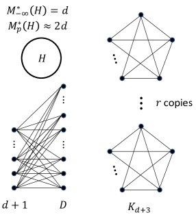
Figure 5: Tight instance for both approximation algorithms from Section 5.

Lemma 5.5.

Let $p\in(-\infty,1)$. Fix $\alpha\in[1,2]$ and an integer $d\geq 1$. Assume there exists a graph $H$ where $d=M_{-\infty}^{*}(H)$ and $M_{p}^{*}(H)\geq\alpha d$. Let $G$ be the disjoint union of (i) $H$, (ii) $r$ copies of a clique on $d+3$ vertices $K_{d+3}$, and (iii) the complete bipartite graph $K_{d+1,D}$ (see Figure 5). Let $n_{H}$ be the number of vertices in $H$. Assume $n_{H}^{2}=o(r)$, $d^{2}=O(D)$ and $dD=o(r)$.

Then (1) $M_{p}^{*}(G)\geq\alpha d$, (2) letting $S_{1}=\mathsf{Simple\text{-}Greedy\text{-}}p(G)$, we have $\displaystyle\lim_{r\to\infty}M_{p}(S_{1})=d+2$ and (3) $\displaystyle\lim_{D\to\infty}M_{p}(M_{1}^{*}(G))=d+1$.

In the graph $G$ in Lemma 5.5, the optimal solution is $H$. When we run $\mathsf{Simple\text{-}Greedy\text{-}}p$ on $G$, $H$ is peeled first and the remainder of the graph has density roughly $d+2$ when there are sufficiently many cliques. For the approximation algorithm from Section 5.2, the densest $1$-mean subgraph of $G$ is $K_{d+1,D}$, which satisfies $M_{p}^{*}(K_{d+1,D})\approx d+1$ for sufficiently large $D$. With more effort, one can argue that, for a fixed $p$ and $\epsilon$, it suffices to take a graph $G$ whose size is polynomial in $D$ and $r$.

With Lemma 5.5, all that remains to prove Theorem 5.4 is to construct a graph $H$ where $d=M_{-\infty}^{*}(H)$ and $M_{p}^{*}(H)\geq(2-\epsilon)d$ for a given $d$ and $\epsilon$.

Theorem 5.6.

Let $\epsilon\in(0,1)$ and $d\geq 1$ be an integer. Assume $p\in(-1,1)$. For all integers $n\geq\frac{2d}{\epsilon}$, there exists a graph $G$ on $n$ vertices with degeneracy $d$ such that $M_{p}^{*}(G)\geq(1-\epsilon)2M_{-\infty}^{*}(G)$.

For $p\in(-\infty,-1]$, we can obtain the same guarantee if $n\geq\frac{\binom{d+1}{2}((1-\frac{1}{2d})^{p}-1)+d(2^{-p}-1)}{\epsilon\cdot\left|p\right|}$.

The proof of the proceeding theorem is constructive, using a result of Bickle [Bic12] to aid in constructing a $d$-degenerate graph where most of the vertices have degree $2d$. Because this graph $G$ has most vertices equal to $2d$, then we expect that $M_{p}^{*}(G)\approx 2d$ as the $M_{p}^{*}$ value of any regular graph is simply the degree of the graph.

Proof of Theorem 5.4.

Theorem 5.6 implies that for sufficiently large $n$, there exists a graph $H$ on $n$ vertices such that $d=M_{-\infty}^{*}(H)$ and $M_{p}^{*}(H)\geq(1-\epsilon)2d$. Therefore, Lemma 5.5 holds with $\alpha=(1-\epsilon)2d$. Thus, there exists an infinite class of graphs where both algorithms from Section 5.1 and 5.2 are at best a $\frac{1}{2}$-approximation. ∎

5.4 Iterative heuristics for $p>1$ and $p<1$

We introduce iterative heuristics for $p>1$ and $p<1$ with the goal of producing better solutions than the algorithms that only consider a single ordering of the vertices.

For $p>1$, recall that the algorithm $\mathsf{Greedy}\nolinebreak[4]\raisebox{1.72218pt}{{{++}}}\text{-}p$ converges to a near-optimal solution for $p$-mean DSG. $\mathsf{Greedy}\nolinebreak[4]\raisebox{1.72218pt}{{{++}}}\text{-}p$ runs $\mathsf{Greedy\text{-}}p$ at each iteration, however, this is computationally prohibitive on large graphs. We therefore introduce $\mathsf{Lazy\text{-}Greedy\nolinebreak[4]\raisebox{1.72218pt}{{{++}}}\text{-}}p$, which runs $\mathsf{Lazy\text{-}Greedy\text{-}}p$ at each iteration. We show the benefit of iteration on real-world graphs in Section 7.2.

For $p<1$, we consider a heuristic $\mathsf{Simple\text{-}Greedy\nolinebreak[4]\raisebox{1.72218pt}{{{++}}}\text{-}}p$ that essentially takes the best of both of our approximation algorithms from this section. For the approximation algorithm from Section 5.2 that returns the $1$-mean densest subgraph, we use the algorithm $\mathsf{Greedy}\nolinebreak[4]\raisebox{1.72218pt}{{{++}}}$ to compute a near-optimal solution $S_{1}$ to $1$-mean DSG. Our heuristic $\mathsf{Simple\text{-}Greedy\nolinebreak[4]\raisebox{1.72218pt}{{{++}}}\text{-}}p$ runs $\mathsf{Greedy}\nolinebreak[4]\raisebox{1.72218pt}{{{++}}}$ and finds the largest $M_{p}$-density suffix of all orderings produced by $\mathsf{Greedy}\nolinebreak[4]\raisebox{1.72218pt}{{{++}}}$. This implies that the first iteration of $\mathsf{Simple\text{-}Greedy\nolinebreak[4]\raisebox{1.72218pt}{{{++}}}\text{-}}p$ is exactly $\mathsf{Simple\text{-}Greedy\text{-}}p$. As we use $\mathsf{Greedy}\nolinebreak[4]\raisebox{1.72218pt}{{{++}}}$ for computing $S_{1}$, we have that $\mathsf{Simple\text{-}Greedy\nolinebreak[4]\raisebox{1.72218pt}{{{++}}}\text{-}}p$ produces a subgraph that has density at least as good as both of our approximation algorithms. It could even potentially produce a larger density as it considers many more orderings than just the ones that correspond to $S_{-\infty}^{*}$ and $S_{1}$. We run experiments testing the benefit of iteration on real-world graphs in Section 7.2.

6 Hardness of $p$-mean DSG

The goal of this section is to prove the following theorem.

Theorem 6.1.

$p$-mean DSG is NP-hard for $p\in(-\frac{1}{8},0)\cup(0,\frac{1}{4})$ and weighted $p$-mean DSG is NP-hard for $p\in(-3,0)\cup(0,1)$.

In this section, we present our hardness results for $p>0$. In the appendix, we discuss how one can formally extend the arguments to $p<0$ (see Appendix D.2) and we informally discuss how to extend the argument for more values of $p$ in $(-\infty,0)\cup(0,1)$ (see Appendix D.3).

Let $p\in(0,1)$. Recall $f_{p}(S)=\sum_{v\in S}d_{S}(v)^{p}$ and $\rho_{p}(S)=\frac{f_{p}(S)}{\left|S\right|}$. As $p>0$, $\max_{S}M_{p}(S)$ is equivalent to the problem of $\max_{S}\rho_{p}(S)$. We therefore focus on the problem of $\max_{S}\rho_{p}(S)$. We give a reduction from the standard NP-Complete problem Exact $3$-Cover.

Problem 6.2 (Exact $3$-Cover).

In the Exact $3$-Cover problem, the input is a family of subsets $\mathcal{S}=\{S_{1},S_{2},\ldots,S_{m}\}$ each of cardinality $3$ over a ground set $\mathcal{U}=\{e_{1},e_{2},\ldots,e_{3n}\}$ and the goal is to determine if there exists a collection of sets $S_{i_{1}},S_{i_{2}},\ldots,S_{i_{n}}$ that form a partition of $\mathcal{U}$. If such sets exist, we say that $\{S_{i_{1}},\ldots,S_{i_{n}}\}$ is an exact $3$-cover.

We give a formal definition of weighted $p$-mean DSG.

Problem 6.3 (weighted $p$-mean DSG).

The input is an edge-weighted graph $G=(V,E,c:E\to\mathbb{R}_{+})$. The weighted $p$-mean DSG problem is the same as the $p$-mean DSG problem if one defines $d_{S}(v)$ as the weighted degree $\sum_{e\in\delta(v)\cap E(S)}c_{e}$ where $\delta(v)$ is the set of edges leaving $v$.

The reduction from Exact $3$-Cover.

We first give the reduction for the weighted case. Let $\mathcal{S}=\{S_{1},S_{2},\ldots,S_{m}\}$ and $\mathcal{U}=\{e_{1},\ldots,e_{3n}\}$ be an instance of Exact $3$-Cover. We first construct a graph $G=(L\cup A,E)$ as follows. $L$ has a vertex $v_{i}$ for each set $S_{i}$ and $A$ has a vertex $u_{j}$ for each element $e_{j}$. We add a weight $1$ edge from every “set vertex" in $L$ to the corresponding “element vertices" in $A$ that the set contains. Formally, for all $i\in[m]$, we add the edge set $\{(v_{i}u_{j},1)\mid e_{j}\in S_{i}\}$ to $E$ where $(v_{i}u_{j},1)$ is the undirected edge from $v_{i}$ to $u_{j}$ of weight $1$. Further, we add an edge to $E$ between all pairs of vertices in $A$ with weight $\frac{d}{\left|A\right|-1}$ where $d:=1.23p+4.77$. Let $\rho^{*}:=\frac{3^{p}+3(d+1)^{p}}{4}$ and let $\mathsf{OPT}_{G}=\operatorname*{arg\,max}_{S}\rho_{p}(S)$. The reduction constructs this graph and returns TRUE iff $\mathsf{OPT}_{G}\geq\rho^{*}$. We provide an illustration of the reduction in Figure 6. The weights of the edges in our reduction are rational numbers and could be made integral by scaling the edge weights by an appropriate integer. One could then argue that an unweighted version of the problem defined with multigraphs is NP-Hard.

For the reduction for the unweighted case, we again construct the graph $G=(L\cup A,E)$. All weight-$1$ edges from $L$ to $A$ remain but now they are unweighted. Instead of $G[A]$ being a clique with equal weight edges, we let $G[A]$ be a connected $d$-regular graph where $d=5$. (We can assume $n$ is even so that such a $d$-regular graph must exist.) Again, the reduction constructs this graph $G$ and returns TRUE iff $\mathsf{OPT}_{G}\geq\rho^{*}$.

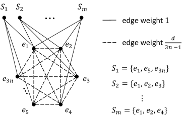
Figure 6: Graph constructed in our reduction from Exact $3$-Cover. The Exact $3$-Cover instance is the family of sets $\{S_{1},\ldots,S_{m}\}$ defined over the ground set $\{e_{1},\ldots,e_{3n}\}$.

Proof outline.

The degree of the vertices in $A$ in the subgraph $G[A]$ is $d=1.23p+4.77$ for the weighted case and $d=5$ for the unweighted case, which are both larger than the degree-$3$ vertices in $L$. $d$ is chosen to be large enough in both cases so that any optimal solution will necessarily take all of $A$, but small enough so that optimal solutions still need to take vertices in $L$. Considering only subsets $S\subseteq L$ of a fixed size, the objective function $\rho_{p}(S\cup A)$ favors solutions $S\cup A$ with more uniform degrees. We take advantage of this to show that an exact 3-cover, which will add exactly one to the degree of each vertex in $A$, attains the largest possible density $\rho^{*}$.

Now suppose $\mathcal{S}$ contains an exact $3$-cover $S_{i_{1}},\ldots,S_{i_{n}}$. Let $S=\{v_{i_{1}},\ldots,v_{i_{n}}\}$ be the subset of $L$ corresponding to the exact $3$-cover. Then as $\left|S\right|=n=\frac{\left|A\right|}{3}$,

$$\mathsf{OPT}_{G}\geq\frac{f_{p}(S\cup A)}{\left|S\cup A\right|}=\frac{3^{p}\cdot\left|S\right|+(d+1)^{p}\left|A\right|}{\left|S\right|+\left|A\right|}\\ =\frac{3^{p}\cdot\frac{\left|A\right|}{3}+(d+1)^{p}\left|A\right|}{\frac{\left|A\right|}{3}+\left|A\right|}=\rho^{*}.$$ (5)

Now assume $\mathcal{S}$ does not contain an exact $3$-cover. Letting $S\subseteq L$ and $A^{\prime}\subseteq A$, we want to show that $\rho_{p}(S\cup A^{\prime})<\rho^{*}$. We focus on the case where $A^{\prime}=A$. Suppose $3\cdot\left|S\right|=\alpha\left|A\right|$ for some $\alpha\in\mathbb{R}_{\geq 0}$. We then have

$$\rho_{p}(S\cup A) =\frac{3^{p}\cdot\left|S\right|+\sum_{v\in A}d_{S\cup A}(v)^{p}}{\left|S\right|+\left|A\right|}$$ (6)

$$=\frac{3^{p}\cdot\left|S\right|+\sum_{v\in A}(d+d_{S+v}(v))^{p}}{\left|S\right|+\left|A\right|}$$ (7)

$$\leq\frac{3^{p}\cdot\left|S\right|+\left|A\right|\cdot(d+\frac{3\left|S\right|}{\left|A\right|})^{p}}{\left|S\right|+\left|A\right|}$$ (8)

$$=\frac{3^{p}\cdot\alpha+3\cdot(d+\alpha)^{p}}{\alpha+3},$$ (9)

where the first equality holds as $G[A]$ is $d$-regular, the inequality uses the fact that $\sum_{i=1}^{n}(d+x_{i})^{p}$ is a concave function in $x$ and, subject to the constraint that $\sum_{i}x_{i}=s$, is maximized when each $x_{i}=\frac{s}{n}$, and the final equality holds as $3\cdot\left|S\right|=\alpha\left|A\right|$. Define

$$g(\alpha):=\frac{3^{p}\cdot\alpha+3\cdot(d+\alpha)^{p}}{\alpha+3}.$$

Note that $g(1)=\rho^{*}$.

We claim it suffices to choose $d$ such that $g(\alpha)$ is uniquely maximized at $\alpha=1$. So if $\alpha\neq 1$, then $\rho_{p}(S\cup A)<g(1)$ by the choice of $d$. Now consider the case when $\alpha=1$. As $\mathcal{S}$ does not contain an exact $3$-cover, it must be the case that there exists $u,v\in A$ such that $d_{S\cup A}(u)\neq d_{S\cup A}(v)$. This implies that Inequality (8) is strict, which again implies $\rho_{p}(S\cup A)<g(1)$.

A natural direction for the proof would then be to choose $d$ so that $g(\alpha)$ is uniquely maximized at $\alpha=1$. The main issue with this approach is that it leads to solutions where $d$ is irrational even when $p$ is rational. One might think we should then consider reducing from Exact $l$-Cover where $\ell>3$ is an integer. However, it is a challenging problem to choose such an $\ell$ and $d$.

To remedy these issues, in Lemma 6.4, we consider a tighter bound than the one in Inequality (8), which utilizes the fact that we are optimizing the function of interest over the integers. We provide a proof of the lemma in Appendix D.

Lemma 6.4.

Let $c\in\mathbb{R}_{\geq 0}$ and $p>0$. Let $f:\mathbb{R}_{\geq 0}^{n}\to\mathbb{R}$ be defined as $f(x)=\sum_{i=1}^{n}(c+x_{i})^{p}$ where $x\in\mathbb{R}^{n}$ and $x_{i}$ is the $i$-th coordinate of $x$. Consider the program parameterized by $s\in\mathbb{N}$:

$$\text{maximize }f(x)\text{ over }x\in\mathbb{Z}^{n},x\geq 0\text{ s.t. }\sum_{i=1}^{n}x_{i}=s.$$

The program is uniquely maximized at the vector of integers with sum equal to $s$ and each entry is in $\{\left\lceil s/n\right\rceil,\left\lceil s/n\right\rceil-1\}$.

If $p<0$ and the optimization problem is a minimization problem, the program is uniquely minimized at the vector of integers with sum equal to $s$ and each entry is in $\{\left\lceil s/n\right\rceil,\left\lceil s/n\right\rceil-1\}$.

Now consider again the case when the input $\mathcal{S}$ does not contain an exact 3-cover. From the proof outline above, we want to argue that the quantity in (7) is strictly less than $g(1)$, which is equal to $\rho^{*}$. Reevaluating (7) with Lemma 6.4 in hand, we have a tighter bound on $\sum_{v\in A}(d+d_{S+v}(v))^{p}$ compared to the bound in (8) as $d_{S+v}(v)$ is integral for all $v\in A$. After carefully choosing the value of $d$, this improved bound allows us to prove that the quantity in (7) is strictly less than $g(1)$.

We use the proof outline above to prove the following theorem, which is exactly Theorem 6.1 when assuming $p>0$.

Theorem 6.5.

$p$-mean DSG is NP-hard for $p\in(0,\frac{1}{4})$ and weighted $p$-mean DSG is NP-hard for $p\in(0,1)$.

We note again that we prove NP-hardness for values of $p<0$ in the appendix (see Appendix D.2).

7 Experiments

We evaluate the algorithms described in previous sections on ten real-world graphs. The graphs are publicly accessible from SNAP [LK14] and SuiteSparse Matrix Collection [DH11]. The size of each graph is given in Table 1. The graphs we consider are a subset of the graphs from [VBK21]. We focused on the graphs in [VBK21] for which they reported raw statistics, which was done purposefully to facilitate direct comparisons. Some graphs vary slightly from the graphs in [VBK21] due to differences in preprocessing as we remove all isolated vertices.

All algorithms are implemented in C++. We use the implementation of $\mathsf{Greedy}\nolinebreak[4]\raisebox{1.72218pt}{{{++}}}$ from [BGP⁺20], which serves as our implementation for $\mathsf{Simple\text{-}Greedy\text{-}}p$ and $\mathsf{Simple\text{-}Greedy\nolinebreak[4]\raisebox{1.72218pt}{{{++}}}\text{-}}p$. We did not use the implementation for $\mathsf{Greedy\text{-}}p$ of [VBK21] as it was written in Julia. The reported running times of $\mathsf{Greedy\text{-}}p$ in [VBK21] are roughly twice as fast as our implementation. This difference largely does not impact our results and we mention why this is the case in each section. We do not measure the time it takes to read the graph in order to reduce variability (the time it takes to read the largest graph is 6 seconds). The experiments were done on a Slurm-based cluster, where we ran each experiment on 1 node with 16 cores. Each node/core had Xeon PHI 5100 CPUs and 16 GB of RAM.

In each section, we present partial results for a few graphs but include all results in the appendix (see Appendix E). We give a few highlights here and discuss details in the following sections.

• For $p>1$, $\mathsf{Lazy\text{-}Greedy\text{-}}p$ is much faster than $\mathsf{Greedy\text{-}}p$ while returning subgraphs with comparable density.

• For $\mathsf{Lazy\text{-}Greedy\nolinebreak[4]\raisebox{1.72218pt}{{{++}}}\text{-}}p$ with $p>1$, multiple iterations improve upon the density of $\mathsf{Lazy\text{-}Greedy\text{-}}p$ for some graphs.

• For $p<1$, $\mathsf{Simple\text{-}Greedy\text{-}}p$ returns solutions with similar density to the algorithms we compare it against but runs significantly faster.

	Astro	CM05	BrKite	Enron	roadCA
$n$	18,771	39,577	58,228	36,692	1,965,206
$m$	198,050	175,693	214,078	183,831	2,766,607

	roadTX	webG	webBS	Amaz	YTube
$n$	1,379,917	875,713	685,230	334,863	1,134,890
$m$	1,921,660	4,322,051	6,649,470	925,872	2,987,624

Table 1: Sizes of the real-world graphs used in experiments.

7.1 $\mathsf{Lazy\text{-}Greedy\text{-}}p$ outperforms $\mathsf{Greedy\text{-}}p$

metric	algorithm	Astro	roadCA	webBS	YTube
time (s)	$\mathsf{Lazy\text{-}G\text{-}}p$ ($\epsilon$$=$$0.1$)	0.144	3.148	13.32	7.685
	$\mathsf{Lazy\text{-}G\text{-}}p$ ($\epsilon$$=$$1.0$)	0.105	3.196	9.952	4.623
	$\mathsf{Greedy\text{-}}p$	0.312	3.146	687.2	75.98
density ($M_{p}$)	$\mathsf{Lazy\text{-}G\text{-}}p$ ($\epsilon$$=$$0.1$)	61.6	3.756	207.4	95.5
	$\mathsf{Lazy\text{-}G\text{-}}p$ ($\epsilon$$=$$1.0$)	61.76	3.756	207.4	95.5
	$\mathsf{Greedy\text{-}}p$	61.6	3.683	207.4	95.5

(a) Results for $p=1.25$

metric	algorithm	Astro	roadCA	webBS	YTube
time (s)	$\mathsf{Lazy\text{-}G\text{-}}p$ ($\epsilon$$=$$0.1$)	0.157	3.135	14.16	6.931
	$\mathsf{Lazy\text{-}G\text{-}}p$ ($\epsilon$$=$$1.0$)	0.108	3.104	9.931	4.044
	$\mathsf{Greedy\text{-}}p$	0.31	3.219	742.4	68.5
density ($M_{p}$)	$\mathsf{Lazy\text{-}G\text{-}}p$ ($\epsilon$$=$$0.1$)	67.12	3.816	387.1	112.2
	$\mathsf{Lazy\text{-}G\text{-}}p$ ($\epsilon$$=$$1.0$)	67.88	3.769	387.1	112.2
	$\mathsf{Greedy\text{-}}p$	67.12	3.816	387.1	112.2

(b) Results for $p=1.75$

Table 2: Wall clock times and densities of returned solutions of $\mathsf{Lazy\text{-}Greedy\text{-}}p$ and $\mathsf{Greedy\text{-}}p$ on four of the ten graphs and for $p\in\{1.25,1.75\}$. We write $\mathsf{Lazy\text{-}Greedy\text{-}}p$ as $\mathsf{Lazy\text{-}G\text{-}}p$ for spacing issues. Results for all ten graphs and more values of $p$ are in Appendix E.

We find that $\mathsf{Lazy\text{-}Greedy\text{-}}p$ outperforms $\mathsf{Greedy\text{-}}p$ in terms of running time and typically returns a solution with similar density. We run experiments for $p\in\{1.05,1.25,1.5,1.75,2\}$. Note that we stop at $p=2$ as the objective starts rewarding subgraphs with large degrees and therefore the returned subgraphs are often a large fraction of the graph. We evaluate $\mathsf{Lazy\text{-}Greedy\text{-}}p$ with values of $\epsilon\in\{0.01,0.1,1\}$, all of which result in similar running times and densities. In Table 2, we present the running times and densities of returned solutions for $\mathsf{Lazy\text{-}Greedy\text{-}}p$ and $\mathsf{Greedy\text{-}}p$ on four of the ten real-world graphs and for two values of $p$. The full table of the results is given in Appendix E.

Ignoring the road networks roadCA and roadTX, $\mathsf{Lazy\text{-}Greedy\text{-}}p$ is roughly at least twice as fast as $\mathsf{Greedy\text{-}}p$. The road networks have a maximum degree of 12, so the savings from $\mathsf{Lazy\text{-}Greedy\text{-}}p$ are marginal. On graphs webG and webBS, $\mathsf{Lazy\text{-}Greedy\text{-}}p$ is roughly at least $4$ times faster. Since webG and webBS have many vertices of large degree, this was expected as we know from the analysis of $\mathsf{Lazy\text{-}Greedy\text{-}}p$, the running time of $\mathsf{Greedy\text{-}}p$ depends on the sum of the squared degrees. We therefore suggest the use of $\mathsf{Lazy\text{-}Greedy\text{-}}p$ over $\mathsf{Greedy\text{-}}p$, especially for graphs with large degrees, which we expect in many real-world graphs. We also point out that the reported running time difference with [VBK21] does not impact these results as this is a relative comparison; we use the same code for $\mathsf{Greedy\text{-}}p$ and $\mathsf{Lazy\text{-}Greedy\text{-}}p$ where the only difference is when the $f_{p}(v\mid S-v)$ values in the min-heap are updated.

7.2 Finding near-optimal solutions for $p>1$

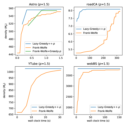
Figure 7: Results for convergence of iterative algorithms for finding near-optimal solutions where $p=1.5$ on four of the ten real-world graphs. Results for all ten graphs and more values of $p$ are in Appendix E.

We compare $\mathsf{Lazy\text{-}Greedy\nolinebreak[4]\raisebox{1.72218pt}{{{++}}}\text{-}}p$, $\mathsf{Greedy}\nolinebreak[4]\raisebox{1.72218pt}{{{++}}}\text{-}p$, and the Frank-Wolfe method in terms of running time and solution quality. In [HQC22], Harb et al. show how one can use Frank-Wolfe to solve an appropriate convex programming relaxation of $p$-mean DSG. We provide details of the algorithm in the appendix (see Appendix E).

We run $\mathsf{Lazy\text{-}Greedy\nolinebreak[4]\raisebox{1.72218pt}{{{++}}}\text{-}}p$ and $\mathsf{Greedy}\nolinebreak[4]\raisebox{1.72218pt}{{{++}}}\text{-}p$ for $100$ iterations and Frank-Wolfe for $500$ iterations. We only run $\mathsf{Greedy}\nolinebreak[4]\raisebox{1.72218pt}{{{++}}}\text{-}p$ on the five smallest graphs for even if we used the faster implementation of $\mathsf{Greedy\text{-}}p$ in [VBK21], the running time on large graphs could reach roughly around ten hours. Thus, for large graphs, this points to $\mathsf{Lazy\text{-}Greedy\nolinebreak[4]\raisebox{1.72218pt}{{{++}}}\text{-}}p$ and Frank-Wolfe being better options than $\mathsf{Greedy}\nolinebreak[4]\raisebox{1.72218pt}{{{++}}}\text{-}p$. For $\mathsf{Lazy\text{-}Greedy\nolinebreak[4]\raisebox{1.72218pt}{{{++}}}\text{-}}p$, we set $\epsilon=1$. We run experiments for $p\in\{1.05,1.25,1.5,1.75,2\}$. In Figure 7, we present plots showing the rate of convergence for four of the ten real-world graphs with $p=1.5$. For each plot, we truncated the data to the first point at which all algorithms reached at least $99\%$ of the optimal density achieved in order to more easily see trends in the data. The full collection of results is given in Appendix E.

We find there is a benefit to iteration; $\mathsf{Lazy\text{-}Greedy\nolinebreak[4]\raisebox{1.72218pt}{{{++}}}\text{-}}p$ produces solutions with increasing density for multiple iterations for around half of the graphs (e.g., see roadCA and Astro plots in Figure 7). We also note that the rate of convergence of $\mathsf{Lazy\text{-}Greedy\nolinebreak[4]\raisebox{1.72218pt}{{{++}}}\text{-}}p$ is faster than Frank-Wolfe on almost every single graph.

7.3 Approximation algorithms for $p<1$

metric	algorithm	Astro	roadCA	webBS	YTube
time (s)	$\mathsf{Simple\text{-}G\text{-}}p$	0.022	1.146	0.836	1.151
	1-mean DSG	2.179	164.9	76.95	117.9
	$\mathsf{Simple\text{-}G\nolinebreak[4]\raisebox{1.72218pt}{{{++}}}\text{-}}p$	2.179	164.9	76.95	117.9
density ($M_{p}$)	$\mathsf{Simple\text{-}G\text{-}}p$	56.91	3.27	204.0	75.56
	1-mean DSG	55.52	3.583	204.0	72.8
	$\mathsf{Simple\text{-}G\nolinebreak[4]\raisebox{1.72218pt}{{{++}}}\text{-}}p$	58.92	3.75	204.0	75.56

(a) Results for $p=-1$

metric	algorithm	Astro	roadCA	webBS	YTube
time (s)	$\mathsf{Greedy\text{-}}p$	1.553	4.364	4483.8	292.3
	$\mathsf{Simple\text{-}G\text{-}}p$	0.036	0.857	1.31	0.887
	1-mean DSG	3.772	99.07	124.0	90.44
	$\mathsf{Simple\text{-}G\nolinebreak[4]\raisebox{1.72218pt}{{{++}}}\text{-}}p$	3.772	99.07	124.0	90.44
density ($M_{p}$)	$\mathsf{Greedy\text{-}}p$	56.86	3.296	205.9	85.28
	$\mathsf{Simple\text{-}G\text{-}}p$	57.48	3.333	205.9	85.23
	1-mean DSG	61.59	3.848	205.9	84.74
	$\mathsf{Simple\text{-}G\nolinebreak[4]\raisebox{1.72218pt}{{{++}}}\text{-}}p$	61.87	3.867	205.9	85.24

(b) Results for $p=0.5$

Table 3: Wall clock times and densities of returned solutions for the algorithms we tested for $p\in\{-1,0.5\}$. We write $\mathsf{Simple\text{-}Greedy\text{-}}p$ as $\mathsf{Simple\text{-}G\text{-}}p$ and $\mathsf{Simple\text{-}Greedy\nolinebreak[4]\raisebox{1.54996pt}{{{++}}}\text{-}}p$ as $\mathsf{Simple\text{-}G\nolinebreak[4]\raisebox{1.54996pt}{{{++}}}\text{-}}p$ for spacing issues. Results for all ten graphs and more values of $p$ are in Appendix E.

For $p<1$, we evaluate our two approximation algorithms from Section 5, $\mathsf{Greedy\text{-}}p$, and the heuristic $\mathsf{Simple\text{-}Greedy\nolinebreak[4]\raisebox{1.72218pt}{{{++}}}\text{-}}p$ described in Section 5.4. We run all four algorithms on all ten real-world graphs and for $p\in\{0.25,0.5,0.75\}$. We only run our approximation algorithms and $\mathsf{Simple\text{-}Greedy\nolinebreak[4]\raisebox{1.72218pt}{{{++}}}\text{-}}p$ for $p\in\{-1,-0.5\}$ as $\mathsf{Greedy\text{-}}p$ is not well-defined for $p<0$. We run $\mathsf{Simple\text{-}Greedy\nolinebreak[4]\raisebox{1.72218pt}{{{++}}}\text{-}}p$ for 100 iterations. For our approximation algorithm returning the $1$-mean DSG, as noted in Section 5.4, we use $\mathsf{Greedy}\nolinebreak[4]\raisebox{1.72218pt}{{{++}}}$ to compute a near-optimal solution. In Table 3, we present the results for four of the ten graphs and for two values of $p$. The full table of results is given in Appendix E.

We first want to highlight the fact that the orderings produced by $\mathsf{Simple\text{-}Greedy\text{-}}p$ and $\mathsf{Simple\text{-}Greedy\nolinebreak[4]\raisebox{1.72218pt}{{{++}}}\text{-}}p$ are not dependent on $p$. One can therefore run these algorithms once to compute approximations to $p$-mean DSG for many different values of $p<1$.

For values of $p\in(0,1)$, all four algorithms return graphs with roughly the same density, however, $\mathsf{Simple\text{-}Greedy\text{-}}p$ is much faster than the other three algorithms. As $\mathsf{Simple\text{-}Greedy\text{-}}p$ is only $1$ iteration of $\mathsf{Simple\text{-}Greedy\nolinebreak[4]\raisebox{1.72218pt}{{{++}}}\text{-}}p$ and we run $\mathsf{Simple\text{-}Greedy\nolinebreak[4]\raisebox{1.72218pt}{{{++}}}\text{-}}p$ for $100$ iterations, we find that $\mathsf{Simple\text{-}Greedy\text{-}}p$ is roughly around $100$ times faster than $\mathsf{Simple\text{-}Greedy\nolinebreak[4]\raisebox{1.72218pt}{{{++}}}\text{-}}p$ and the algorithm finding the 1-mean densest subgraph. Furthermore, $\mathsf{Simple\text{-}Greedy\text{-}}p$ is anywhere from $2$ to $20$ times as fast as $\mathsf{Greedy\text{-}}p$. For values of $p<0$, $\mathsf{Simple\text{-}Greedy\text{-}}p$ again performs the best as it returns subgraphs of comparable density and is also the fastest algorithm. We also want to point out that although $\mathsf{Simple\text{-}Greedy\nolinebreak[4]\raisebox{1.72218pt}{{{++}}}\text{-}}p$ sometimes produces subgraphs with larger density than all algorithms tested, the benefit of iteration with $\mathsf{Simple\text{-}Greedy\nolinebreak[4]\raisebox{1.72218pt}{{{++}}}\text{-}}p$ is marginal.

8 Conclusion

In this paper, we provide a deeper understanding of $p$-mean DSG for the entire range of $p$. For $p\in(-\frac{1}{8},0)\cup(0,\frac{1}{4})$, we show $p$-mean DSG is NP-Hard via a nontrivial reduction and we show how to extend this NP-hardness proof to $p\in(-3,0)\cup(0,1)$ for the weighted version of the problem. This mostly resolves the open question regarding the complexity of $p$-mean DSG for $p<1$. We presented two approximation algorithms for $p<1$, which are the first algorithms with any provable approximation ratio for this regime of $p$. We provided a faster implementation of $\mathsf{Greedy\text{-}}p$ for $p>1$ called $\mathsf{Lazy\text{-}Greedy\text{-}}p$. We developed a heuristic based on iterative algorithms for finding near-optimal solutions to $p$-mean DSG that utilized $\mathsf{Lazy\text{-}Greedy\text{-}}p$. This algorithm is ideal when $\mathsf{Lazy\text{-}Greedy\text{-}}p$ does not find a near-optimal solution after a single iteration. Experiments show that our approximation algorithms for both $p>1$ and $p<1$ are highly effective and scalable.

We outline a few future directions. We established NP-Hardness for $p$-mean DSG where $p\in(-\frac{1}{8},0)\cup(0,\frac{1}{4})$ and for weighted $p$-mean DSG where $p\in(-3,0)\cup(0,1)$ and also provided simple $1/2$-approximation algorithms. We believe that our NP-Hardness proof can be strengthened to show that it is APX-Hard to approximate the optimum, that is, there is some fixed $\delta>0$ such that it is NP-Hard to obtain a $(1-\delta)$-approximation. The resulting $\delta$ is likely to be quite small. It is important to obtain tight approximation bounds for $p$-mean DSG that closes that gap between $1/2$ and $(1-\delta)$. This effort is likely to lead to the development of more sophisticated approximation algorithms and heuristics for the problem.

Acknowledgements.

The authors would like to thank Farouk Harb for helpful discussions and for providing code for the Frank-Wolfe algorithm.

Appendix A Omitted Proofs from Section 3

Proposition 3.1 is folklore and we only include the following proof for the sake of completeness.

Proof of Proposition 3.1.

It suffices to show that $M_{p}(S)$ is an increasing function in $p$ for a fixed $S$. Fix $S\subseteq V$ and assume $p\not\in\{-\infty,0,\infty\}$. We have

$$\frac{d}{dp}\,M_{p}(S) =M_{p}(S)\cdot\frac{d}{dp}\,\ln M_{p}(S)$$

$$\geq\frac{d}{dp}\,\ln M_{p}(S)$$

$$=-\frac{1}{p^{2}}\ln\rho_{p}(S)+\frac{1}{p\cdot f_{p}(S)}\cdot\frac{d}{dp}\,f_{p}(S)$$

$$=-\frac{1}{p^{2}}\ln\rho_{p}(S)+\frac{1}{p}\cdot\frac{\sum_{v\in S}d_{S}(v)^{p}\ln d_{S}(v)}{\sum_{v\in S}d_{S}(v)^{p}}$$ (10)

where (10) is at least $0$ if and only if

$$\ln\rho_{p}(S)\leq\frac{\sum_{v\in S}d_{S}(v)^{p}\ln d_{S}(v)^{p}}{\sum_{v\in S}d_{S}(v)^{p}}.$$ (11)

Rearranging, (11) is equivalent to

$$\ln(1/\left|S\right|)\leq\sum_{v\in S}x_{v}\ln x_{v}$$

where $x_{v}:=\frac{d_{S}(v)^{p}}{\sum_{v\in S}d_{S}(v)^{p}}$. As $x$ is a probability distribution over $S$, the final inequality holds by recognizing that the uniform distribution maximizes the entropy function. Thus, $M_{p}(S)$ is an increasing function in $p$ over $(-\infty,0)$ and $(0,\infty)$. One can extend the proof for $p\in\{-\infty,0,\infty\}$ by recognizing that the definition for $M_{p}(S)$ in these cases is derived by taking the limit (e.g., $\lim_{p\to\infty}M_{p}(S)=M_{\infty}(S)$). This concludes the proof. ∎

Appendix B Omitted Proofs from Section 4

Proof of Lemma 4.2.

We have that $f_{p}$ is supermodular for $p\geq 1$ [VBK21]. Let $S^{*}$ be an optimal subset and $\rho^{*}=\rho_{p}(S^{*})$. In the proof of Theorem 3.1 of [CQT22], it is shown that for all $v\in S^{*}$, $f_{p}(v\mid S^{*}-v)\geq\rho^{*}$.

Let $v_{i}$ be the first element of $S^{*}$ that is peeled. Let $S_{i}$ be the set of vertices including $v_{i}$ and all subsequent vertices in the peeling order. By the update rule in (3), we have $f_{p}(v_{i}\mid S_{i}-v_{i})\leq(1+\epsilon)\min_{u\in S_{i}}f_{p}(u\mid S_{i}-u)$. In Proposition 3.2 of [CQT22], it is shown that for all $S\subseteq V$, we have $\sum_{v\in S}f_{p}(v\mid S-v)\leq(p+1)f(S)$. Repeating the argument in Theorem 3.1 in [CQT22] only with a small change, we have

$$\frac{f_{p}(S_{i})}{\left|S_{i}\right|} =\frac{f_{p}(S_{i})}{\sum_{u\in S_{i}}f(u\mid S_{i}-u)}\cdot\frac{\sum_{u\in S_{i}}f(u\mid S_{i}-u)}{\left|S_{i}\right|}$$

$$\geq\frac{1}{p+1}\cdot\frac{\left|S_{i}\right|\cdot f(v_{i}\mid S_{i}-v_{i})}{(1+\epsilon)\left|S_{i}\right|}$$

$$\geq\frac{\rho^{*}}{(1+\epsilon)(p+1)}$$

$$\geq\frac{(1-\epsilon)\rho^{*}}{p+1}.$$

Raising both sides of the inequality to the $\frac{1}{p}$-th power, we have $M_{p}(S_{i})\geq(\frac{1-\epsilon}{p+1})^{1/p}\cdot M_{p}^{*}$. This concludes the proof. ∎

Proof of Lemma 4.3.

Note that it suffices to consider $\alpha=1+\frac{\epsilon}{p}$ as the left-hand side is increasing in $\alpha$. Consider the function

$$\frac{(\alpha d)^{p}-(\alpha d-1)^{p}}{e^{\epsilon}}.$$ (12)

Suppose we can show this function is decreasing in $\epsilon$. This would imply $\frac{(\alpha d)^{p}-(\alpha d-1)^{p}}{e^{\epsilon}}\leq d^{p}-(d-1)^{p}$, which would prove the statement as $e^{\epsilon}\leq 1+2\epsilon$. We prove that the function is decreasing in $\epsilon$ by arguing that the derivative of (12) with respect to $\epsilon$ is non-positive.

Note that $\frac{d}{d\epsilon}\alpha d=\frac{d}{p}$. We have

$$\frac{d}{d\epsilon}\frac{(\alpha d)^{p}-(\alpha d-1)^{p}}{e^{\epsilon}}=\frac{d[(\alpha d)^{p-1}-(\alpha d-1)^{p-1}]e^{\epsilon}-[(\alpha d)^{p}-(\alpha d-1)^{p}]e^{\epsilon}}{\epsilon^{2\epsilon}}.$$

Since we need this quantity to be non-positive, it suffices to show

$$d\leq\frac{(\alpha d)^{p}-(\alpha d-1)^{p}}{(\alpha d)^{p-1}-(\alpha d-1)^{p-1}}$$

We have

$$\frac{(\alpha d)^{p}-(\alpha d-1)^{p}}{(\alpha d)^{p-1}-(\alpha d-1)^{p-1}}=\alpha d\cdot\frac{1-(1-\frac{1}{\alpha d})^{p}}{1-(1-\frac{1}{\alpha d})^{p-1}}\geq\alpha d\geq d,$$

where the first inequality holds as $(1-\frac{1}{\alpha d})^{p}\leq(1-\frac{1}{\alpha d})^{p-1}$. This concludes the proof. ∎

Proof of Lemma 4.4.

The initialization of $D$ and $D^{\prime}$ takes $O(m)$ time and the initialization of $A$ takes $O(m+n\log n)$ time. At each iteration, as $A$ is a min-heap, finding the minimum and removing it only takes $O(1)$ time and $O(\log n)$ time, respectively. Suppose $v_{i}$ is the vertex chosen at the $i$-th iteration. We consider the first three lines of the inner for loop. The number of iterations of the inner for loop is $O(d_{G}(v_{i}))$ and the first three lines take $O(\log n)$ time. Thus, the total time for these three lines throughout the entire run of the algorithm is $O(m\log n)$ time.

The only part of the algorithm unaccounted for is the conditional statement in the inner for loop. In this if-statement, for a vertex $u$, we update $A[w]$ for all $w\in N(u)\cap S_{i+1}$ only when the approximate degree, $D^{\prime}[u]$, exceeds $(1+\frac{\epsilon}{p})D[u]$, where $D[u]$ is the exact current degree. $u$ is therefore updated only when the actual degree drops by at least a $1+\frac{\epsilon}{p}$ factor. Since $D[u]\leq n$, the maximum number of times we update any vertex is $O(\log_{1+\frac{\epsilon}{p}}(n))$. If $p\geq\epsilon$, this is at most $O(\frac{p\log n}{\epsilon})$. The time it takes to update $A$ is $O(d_{G}(u)\log n)$. Thus, the total time spent on a single vertex $u$ throughout the entire run of the algorithm is $O\left(d_{G}(u)\cdot\frac{\log^{2}n}{\log(1+\frac{\epsilon}{p})}\right)$. This concludes the proof. ∎

Proof of Theorem 4.1..

Running time is analyzed in Lemma 4.4, so we focus on the approximation guarantee. Consider an arbitrary iteration $i$ of the algorithm. By Lemma 4.2, it suffices to show that $f_{p}(v_{i}\mid S_{i}-v_{i})\leq(1+\epsilon)\min_{v\in S_{i}}f_{p}(v\mid S_{i}-v)$. We show something stronger. Let $A_{i}$ be the state of the min-heap $A$ at the start of iteration $i$. We show that for all $v\in S_{i}$, we have $A_{i}[v]\leq(1+\epsilon)f_{p}(v\mid S_{i}-v)$. To prove this, we first note that this holds on the first iteration as we compute the values $f_{p}(v\mid V-v)$ exactly. Let $D_{i}^{\prime}$ be the state of $D^{\prime}$ at the beginning of iteration $i$. As $D$ maintains exact degrees, we use $d_{S_{i}}(v)$ in place of $D[v]$. Note that the algorithm maintains $A$ to ensure $A_{i}[v]=d_{S_{i}}(v)^{p}+\sum_{u\in N(v)\cap S_{i}}D_{i}^{\prime}[u]^{p}-(D_{i}^{\prime}[u]-1)^{p}$. We see that $D^{\prime}[u]\leq(1+\frac{\epsilon}{p})d_{S_{i}}(u)$ is guaranteed for all $u\in S_{i}$ by the condition in the inner for loop of iteration $i-1$ (if $i=1$, then this statement holds as $D_{1}^{\prime}[v]=d_{G}(v)$). Therefore,

$$A_{i}[v]\leq d_{S_{i}}(v)+(1+\epsilon)\sum_{u\in N(v)\cap S_{i}}d_{S_{i}}(u)^{p}-(d_{S_{i}}(u)-1)^{p}$$

by Lemma 4.3. Using the rewriting of $f_{p}(v\mid S_{i}-v)$ given in Equation (2), it follows that $A_{i}[v]\leq(1+\epsilon)f_{p}(v\mid S_{i}-v)$. This concludes the proof. ∎

Appendix C Omitted Proofs from Section 5

Proof of Lemma 5.5.

We start with (1), which follows from the fact that $M_{p}^{*}(H)\geq\alpha d$.

We next prove (2). The algorithm $\mathsf{Simple\text{-}Greedy\text{-}}p$ (from Section 5.1) first peels $H$ as $M_{-\infty}^{*}(H)=d$, then it peels $K_{d+1,D}$, and it finally peels all of the cliques. We have to analyze the density of all suffixes of this ordering and show that all have density at most $d+2$ as $r\to\infty$.

We start by analyzing the suffixes while peeling $H$. Let $H_{i}$ be the remaining vertices from $H$ after peeling $i$ vertices for $i=0,1,\ldots,n_{H}$. Let $T$ be the vertices of $G$ without $H$, so $\left|T\right|=(d+1+D)+r(d+3)$. Thus, on the suffixes while peeling $H$, the algorithm obtains value

$$\max_{i=0,1,\ldots,n_{H}}\left(\frac{\sum_{v\in H_{i}}d_{H_{i}}(v)^{p}+f_{p}(T)}{\left|H_{i}\right|+(d+1+D)+r(d+3)}\right)^{1/p}.$$

We have

$$f_{p}(T)=(d+1)D^{p}+D(d+1)^{p}+r(d+3)(d+2)^{p},$$

so $f_{p}(T)\leq 2(d+1)D+r(d+3)(d+2)^{p}$ and note that $dD=o(r)$. As $\sum_{v\in H_{i}}d_{H_{i}}(v)^{p}\leq n_{H}^{1+p}$ and $n_{H}^{1+p}=o(r)$,

$$\lim_{r\to\infty}\frac{\sum_{v\in H_{i}}d_{H_{i}}(v)^{p}+f_{p}(T)}{\left|H_{i}\right|+(d+1+D)+r(d+3)}=(d+2)^{p}.$$

Thus, as $r\to\infty$, the maximum density attained while peeling $H$ is at most $d+2$.

We next analyze the suffixes while peeling $K_{d+1,D}$. We note that the density achieved while peeling $K_{d+1,D}$ is at most

$$\max_{\begin{subarray}{c}\ell\in[1,d+1]\\ q\in[1,D]\end{subarray}}\left(\frac{\ell q^{p}+q\ell^{p}+r(d+3)(d+2)^{p}}{\ell+q+r(d+3)}\right)^{1/p}.$$

As $\ell q^{p}+q\ell^{p}\leq 2(d+1)D$ and $dD=o(r)$, we have

$$\lim_{r\to\infty}\frac{\ell q^{p}+q\ell^{p}+r(d+3)(d+2)^{p}}{\ell+q+r(d+3)}=(d+2)^{p}.$$

Therefore, $\lim_{r\to\infty}M_{p}(S_{1})=d+1$.

We now prove (3). We start by showing that $M_{1}^{*}(G)$ is $K_{d+1,D}$. We have

$$M_{1}(K_{d+1,D})=\frac{2(d+1)D}{d+1+D}>2d$$

for $D\geq 2d^{2}$. Furthermore, as $M_{-\infty}^{*}(H)=d$, Proposition 3.4 implies that $M_{1}^{*}(H)\leq 2d$. We also have that $M_{1}^{*}(K_{d+3})=d+2$ and $M_{1}(K_{d+1,D})>d+2$ for $D\geq d+6$. Therefore, $M_{1}^{*}(G)=K_{d+1,D}$.

All that remains is to upper bound $M_{p}(K_{d+1,D})$. We have

$$M_{p}(K_{d+1,D}) =\left(\frac{(d+1)D^{p}+D(d+1)^{p}}{d+1+D}\right)^{1/p}.$$

As $p<1$, we have $D^{p}=o(D)$, which implies

$$\lim_{D\to\infty}\frac{(d+1)D^{p}+D(d+1)^{p}}{d+1+D}=(d+1)^{p}.$$

Therefore, $\lim_{D\to\infty}M_{p}(K_{d+1,D})=d+1$. ∎

To prove Theorem 5.6, we construct a graph whose degeneracy is roughly half of the density of an optimal solution to $p$-mean DSGp. Note that Proposition 3.4 shows $M_{p}^{*}\leq 2M_{-\infty}^{*}$. We therefore attempt to construct a $d$-degenerate graph where as many vertices as possible have degree $2d$. Towards this end, we say that a $d$-degenerate graph is edge maximal if adding any edge to the graph makes the graph $(d+1)$-degenerate. The following theorem gives a characterization of edge-maximal $d$-degenerate graphs via degree sequences.

Theorem C.1 ([Bic12]).

Let $d$ be a positive integer. A sequence of positive integers $d_{1}\geq d_{2}\geq\cdots\geq d_{n}$ is the degree sequence of an edge-maximal $d$-degenerate graph if and only if

1. $d\leq d_{i}\leq\min\{n-1,n+d-i\}$ for all $i\in[n]$, and

2. $\sum_{i=1}^{n}d_{i}=2\left(dn-\binom{d+1}{2}\right)$.

We use this theorem of Bickle in the following proof.

Proof of Theorem 5.6.

Consider the following sequence:

$$d,d+1,d+2,\ldots,2d-1,\underbrace{2d-1,2d-1,\ldots,2d-1}_{\text{$\binom{d+1}{2}$ copies}},\underbrace{2d,2d,\ldots,2d}_{\text{$n-d-\binom{d+1}{2}$ copies}}$$

It is easy to check that both conditions (1) and (2) of Theorem C.1 hold. Thus, given such integers $n$ and $d$, we can construct a $d$-degenerate graph on $n$ vertices $G$ with the given degree sequence.

We now argue that $M_{p}(G)\geq(1-\epsilon)2d$, which would prove the theorem. For any $p\in(-\infty,1)\setminus\{0\}$, we have that $M_{p}(G)$ is

$$\left(\frac{(n-d-\binom{d+1}{2})(2d)^{p}+\binom{d+1}{2}(2d-1)^{p}+\sum_{i=0}^{d-1}(d+i)^{p}}{n}\right)^{1/p}$$ (13)

$$\geq\left(\frac{n+\binom{d+1}{2}((1-\frac{1}{2d})^{p}-1)+d(2^{-p}-1)}{n}\right)^{1/p}\cdot 2d,$$ (14)

where we use the fact that $(\frac{a+bx^{p}}{c})^{1/p}$ is an increasing function in $x$ when $x$, $a$, $b$, and $c$ are all positive.

For $p\in(0,1)$, using the rewriting of $M_{p}(G)$ above in (14), we have

$$\frac{M_{p}(G)}{2d}\geq\left(1-\frac{\frac{p(d+1)}{2}+dp}{n}\right)^{1/p}\geq\left(1-\frac{\epsilon(\frac{p(d+1)}{2}+dp)}{2d}\right)^{1/p}\geq 1-\epsilon\cdot\frac{\frac{d+1}{2}+d}{2d}\geq 1-\epsilon,$$

where the first inequality holds as $1-(1-\frac{1}{2d})^{p}\leq\frac{p}{d}$ and $1-2^{-p}\leq p$, the second inequality uses the fact that $n\geq\frac{2d}{\epsilon}$, and the third inequality holds as $(1+x)^{1/p}\geq 1+\frac{x}{p}$ for $x\geq 0$.

Now for $p<0$, again using the rewriting of $M_{p}(G)$ in (14), we have

$$\frac{M_{p}(G)}{2d}\geq\left(1+\frac{\binom{d+1}{2}((1-\frac{1}{2d})^{p}-1)+d(2^{-p}-1)}{n}\right)^{1/p}\geq\left(1+\left|p\right|\cdot\epsilon\right)^{1/p}\geq 1-\epsilon,$$ (15)

where the first inequality holds as $n\geq\frac{\binom{d+1}{2}((1-\frac{1}{2d})^{p}-1)+d(2^{-p}-1)}{\epsilon\cdot\left|p\right|}$, and the last inequality holds as $1-p\cdot\epsilon\leq(1-\epsilon)^{p}$.

If we were to assume $p\in(-1,0)$, from (15) above, we have

$$\frac{\binom{d+1}{2}((1-\frac{1}{2d})^{p}-1)+d(2^{-p}-1)}{\epsilon\cdot\left|p\right|}\leq\frac{\binom{d+1}{2}\frac{\left|p\right|}{d}+2d\left|p\right|}{\epsilon\cdot\left|p\right|}\\ =\frac{\frac{d+1}{2}+d}{\epsilon}\leq\frac{2d}{\epsilon},$$

where the first inequality holds as $(1-\frac{1}{2d})^{p}-1\leq\frac{\left|p\right|}{d}$ and $2^{-p}-1\leq\left|p\right|$. Thus, for the case of $p\in(-1,0)$, it suffices to take $n\geq\frac{2d}{\epsilon}$. This concludes the proof. ∎

Appendix D Omitted Proofs from Section 6

D.1 Hardness for $p\in(0,1)$

We start by providing the proof of Lemma 6.4.

Proof of Lemma 6.4.

Fix $s\in\mathbb{N}$. Let $x^{*}$ be a vector such that $x_{i}^{*}\in\{\left\lceil s/n\right\rceil,\left\lceil s/n\right\rceil-1\}$ for all $i\in[n]$ and $\sum_{i}x_{i}^{*}=s$. Let $x\in\mathbb{Z}^{n}$ and $x\geq 0$ such that $\sum_{i}x_{i}=s$ and at least one entry of $x$ is not in $\{\left\lceil s/n\right\rceil,\left\lceil s/n\right\rceil-1\}$. Let $2r=\sum_{i=1}^{n}\left|x_{i}-x_{i}^{*}\right|$. We prove that $f(x^{*})>f(x)$ by induction on $r$.

For the base case $r=1$, there are three cases to consider. We can handle the first two cases together. In the first case, we have $(x_{1}^{*},x_{2}^{*})=(\left\lceil s/n\right\rceil,\left\lceil s/n\right\rceil)$ and $(x_{1},x_{2})=(\left\lceil s/n\right\rceil+1,\left\lceil s/n\right\rceil-1)$ and $x_{i}=x_{i}^{*}$ for all $i=3,4,\cdots,n$. In the second case, we have $(x_{1}^{*},x_{2}^{*})=(\left\lceil s/n\right\rceil-1,\left\lceil s/n\right\rceil-1)$ and $(x_{1},x_{2})=(\left\lceil s/n\right\rceil,\left\lceil s/n\right\rceil-2)$ and $x_{i}=x_{i}^{*}$ for all $i=3,4,\cdots,n$. For both cases, all we have to show is that $(c+x_{1})^{p}+(c+x_{2})^{p}<(c+x_{1}^{*})^{p}+(c+x_{2}^{*})^{p}$. As $x_{1}^{*}=x_{2}^{*}$, this follows immediately from the fact that the function $\sum_{i=1}^{n}(c+y_{i})^{p}$ is concave in $y$ and, subject to the constraint that $\sum_{i}y_{i}=s$, is maximized when all terms are the same (i.e. $y_{i}=\frac{s}{n}$).

For the third case, $x_{1}=\left\lceil s/n\right\rceil+1$ and $x_{1}^{*}=\left\lceil s/n\right\rceil$, $x_{2}=\left\lceil s/n\right\rceil-2$ and $x_{2}^{*}=\left\lceil s/n\right\rceil-1$, and $x_{i}=x_{i}^{*}$ for all $i=3,4,\ldots,n$. Again, we have to show $(c+x_{1})^{p}+(c+x_{2})^{p}<(c+x_{1}^{*})^{p}+(c+x_{2}^{*})^{p}$. We have $x_{1}>x_{1}^{*}>x_{2}^{*}>x_{2}$. As $(c+x)^{p}$ is concave in $x$ and $x_{1}-x_{1}^{*}=x_{2}^{*}-x_{2}$, we have $(c+x_{1})^{p}-(c+x_{1}^{*})^{p}<(c+x_{2}^{*})^{p}-(c+x_{2})^{p}$. This gives us the inequality we want up to rearranging.

For the inductive step, we assume that the statement holds for $r\geq 1$ and prove that it holds for $r+1$. Suppose that $x\in\mathbb{Z}^{n}$ and $x\geq 0$ such that $\sum_{i}x_{i}=s$, at least one entry of $x$ is not in $\{\left\lceil s/n\right\rceil,\left\lceil s/n\right\rceil-1\}$, and $2(r+1)=\sum_{i=1}^{n}\left|x_{i}-x_{i}^{*}\right|$. Using a similar argument as for the base case, we can reduce $\sum_{i=1}^{n}\left|x_{i}-x_{i}^{*}\right|$ by $2$. This concludes the proof for $p>0$.

For the case of $p<0$, it is easy to see that everything still holds as $\sum_{i=1}^{n}(c+y_{i})^{p}$ is convex in $y$. ∎

In order to prove Theorem 6.5, we first need a few helpful technical lemmas.

Lemma D.1.

Let $d\geq 1$ be an integer and $p\in\mathbb{R}$. Define $h:[0,1]\to\mathbb{R}$ as

$$h(\beta):=\frac{3^{p}\beta+3\beta(d+1)^{p}+3(1-\beta)d^{p}}{\beta+3}.$$

Let $h^{\prime}$ denote the derivative of $h$ with respect to $\beta$. Fix $\beta\in[0,1]$. Then $h^{\prime}(\beta)>0$ if and only if $3^{p}+3(d+1)^{p}>4d^{p}$.

Proof.

We have that $\frac{d}{d\beta}h(\beta)$ is equal to

$$\frac{(3^{p}+3(d+1)^{p}-3d^{p})(\beta+3)-(3^{p}\beta+3\beta(d+1)^{p}+3(1-\beta)d^{p})}{(\beta+3)^{2}}.$$

Simplifying the numerator, $h^{\prime}(\beta)>0$ if and only if

$$3^{1+p}+3^{2}(d+1)^{p}-3^{2}d^{p}-3d^{p}>0.$$

The lemma follows after dividing through by $3$ and rearranging. ∎

Lemma D.2.

Let $d,t\geq 1$ be integers, $p\in\mathbb{R}$, and $\beta\in[0,1]$. Define $g:[0,1]\to\mathbb{R}$ as

$$g(\beta):=\frac{3^{p}(t+\beta)+3\beta(d+t+1)^{p}+3(1-\beta)(d+t)^{p}}{t+\beta+3}.$$

1. Assume $p\in(0,1)$. If $4(d+2)^{p}+3^{p}<5(d+1)^{p}$, then $g$ is strictly decreasing.

2. Assume $p<0$. If $4(d+2)^{p}+3^{p}>5(d+1)^{p}$, then $g$ is strictly increasing.

Proof.

We have $\frac{d}{d\beta}g(\beta)$ is

$$\frac{(3^{p}+3(d+t+1)^{p}-3(d+t)^{p})(t+\beta+3)}{(t+\beta+3)^{2}}\\ -\frac{(3^{p}(t+\beta)+3\beta(d+t+1)^{p}+3(1-\beta)(d+t)^{p})}{(t+\beta+3)^{2}}.$$

Simplifying the numerator of both terms, $\frac{d}{d\beta}g(\beta)<0$ if and only if

$$3t(d+t+1)^{p}-3t(d+t)^{p}+3^{1+p}+3^{2}(d+t+1)^{p}-3^{2}(d+t)^{p}-3(d+t)^{p}<0.$$

Dividing through by $3$ and rearranging, this is equivalent to

$$(4+t)(d+t)^{p}-(3+t)(d+t+1)^{p}-3^{p}>0.$$ (16)

To prove (1), it suffices to show the left-hand side of (16) is increasing in $t$ for $p\in(0,1)$. To prove (2), it suffices to show the left-hand side of (16) is decreasing in $t$ for $p<0$.

Assume $p>0$. The derivative of the left-hand side of (16) with respect to $t$ is

$$(d+t)^{p}+p(4+t)(d+t)^{p-1}-(d+t+1)^{p}-p(3+t)(d+t+1)^{p-1}$$

$$\geq-p(d+t)^{p-1}+p(4+t)(d+t)^{p-1}-p(3+t)(d+t+1)^{p-1}$$

$$=p(3+t)[(d+t)^{p-1}-(d+t+1)^{p-1}]$$

$$\geq 0,$$

where the first inequality follows from the fact that $(x+1)^{p}-x^{p}\leq px^{p-1}$ for all $x>0$ as $x^{p}$ is concave and the second inequality follows from the fact that $x^{p-1}$ is a decreasing function in $x$ as $p<1$. This proves (1).

Now assume $p<0$. As $x^{p}$ is convex in $x$, we have $(x+1)^{p}-x^{p}\geq px^{p-1}$ for all $x>0$. Thus, one can use the same argument as for $p>0$ to show that the derivative of (16) is non-positive. This proves (2). ∎

The following lemma considers the functions

$$3^{p}+3(d+1)^{p}-4d^{p}$$ (17)

and

$$3^{p}+4(d+2)^{p}-5(d+1)^{p},$$ (18)

where $d=1.23p+4.77$ for the weighted case and $d=5$ for the unweighted case. The lemma states that for both the weighted and unweighted cases, (17) is strictly positive and (18) is strictly negative. This is easy to compute explicitly for specific values of $p$; for example, when $p=1/2$ and $d=1.23p+4.77$, the first function has value $\approx 0.0303$ and the second function has value $\approx-0.032$.

One approach to proving the lemma for the weighted case would be to show that the derivative of (17) only has one zero on the interval $[0,1]$ and one can show this critical point is a maximum. Since (17) is $0$ when $p\in\{0,1\}$, this would prove (17) is strictly positive when $p\in(0,1)$. A similar approach can be taken for (18). For the unweighted case, the same proof idea could be used for verifying (18). For (17), one would only have to show the function is strictly increasing over $(0,\frac{1}{4})$. Formal verification of these facts would be quite lengthy and not necessarily illuminating, so we therefore verified these inequalities analytically via MATLAB. To give an idea of what these functions look like, we plot both in Figure 8.

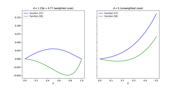
Figure 8: Plot of functions (17) and (18) for different values of $d$.

Lemma D.3.

Let $f_{1}:(0,1)\to\mathbb{R}$ be defined $f_{1}(p)=1.23p+4.77$ and let $f_{2}:(0,\frac{1}{4})\to\mathbb{R}$ be defined $f_{2}(p)=5$. For $i\in\{1,2\}$ and all $p$ in the domain of $f_{i}$, we have

$$3^{p}+3(f_{i}(p)+1)^{p}>4f_{i}(p)^{p}\quad\text{and}\quad 4(f_{i}(p)+2)^{p}+3^{p}<5(f_{i}(p)+1)^{p}.$$

We need one more lemma regarding the general form of the density when solutions in the reduction do not take all of $A$.

Lemma D.4.

Let $G=(L\cup A,E)$ be the graph of the reduction for either the weighted or unweighted case. For the weighted case, assume $p\in(0,1)$ and $d=1.23p+4.77$. For the unweighted case, assume $p\in(0,\frac{1}{4})$ and $d=5$.

Fix $S\subseteq L$ and $A^{\prime}\subseteq A$. Then

$$\rho_{p}(S\cup A^{\prime})=\frac{f_{p}(S\cup A^{\prime})}{\left|S\cup A^{\prime}\right|}\leq\frac{3^{p}\cdot\left|S\right|+\sum_{v\in A^{\prime}}(d+d_{S+v}(v))^{p}}{\left|S\right|+\left|A^{\prime}\right|}$$

If $\left|A^{\prime}\right|<\left|A\right|$, the inequality above is strict.

Proof.

As the degree of each vertex in $S$ is exactly $3$ in both the weighted and unweighted cases,

$$\rho_{p}(S\cup A^{\prime})=\frac{f_{p}(S\cup A^{\prime})}{\left|S\cup A^{\prime}\right|}=\frac{3^{p}\cdot\left|S\right|+\sum_{v\in A^{\prime}}d_{S\cup A^{\prime}}(v)^{p}}{\left|S\right|+\left|A^{\prime}\right|}.$$

In the weighted case, for all $v\in A^{\prime}$, $d_{S\cup A^{\prime}}(v)^{p}=\left(d\cdot\frac{\left|A^{\prime}\right|-1}{\left|A\right|-1}+d_{S+v}(v)\right)^{p}$. As $x^{p}$ is a strictly increasing function in $x$, we have $d_{S\cup A^{\prime}}(v)^{p}\leq(d+d_{S+v}(v))^{p}$. If $\left|A^{\prime}\right|<\left|A\right|$, then the inequality is strict. In the unweighted case, as $G[A]$ is $d$-regular, then $d_{S\cup A^{\prime}}(v)^{p}\leq(d+d_{S+v}(v))^{p}$ for all $v\in A^{\prime}$. If $\left|A^{\prime}\right|<\left|A\right|$, as $G[A]$ is connected, there must exist a vertex $u\in A^{\prime}$ such that $d_{A^{\prime}}(u)\leq 4<d$. Thus, $d_{S\cup A^{\prime}}(u)^{p}<(d+d_{S+u}(u))^{p}$. Therefore, in both the weighted and unweighted cases, we have $\sum_{v\in A^{\prime}}d_{S\cup A^{\prime}}(v)^{p}\leq\sum_{v\in A^{\prime}}(d+d_{S+v}(v))^{p}$, where the inequality is strict if $\left|A^{\prime}\right|<\left|A\right|$. This concludes the proof. ∎

We are now ready to prove Theorem 6.5.

Proof of Theorem 6.5.

Consider an instance of the Exact $3$-Cover problem: let $\mathcal{S}=\{S_{1},\ldots,S_{m}\}$ be a family of subsets of the ground set $\mathcal{U}=\{e_{1},e_{2},\ldots,e_{3n}\}$. We use the reductions given in Section 6 for the weighted and unweighted cases. Recall that both reductions construct the graph $G=(L\cup A,E)$ and return TRUE iff $\mathsf{OPT}_{G}\geq\rho^{*}$ where $\rho^{*}=\frac{3^{p}+3(d+1)^{p}}{4}$. Note $d=1.23p+4.77$ for the weighted case and $d=5$ for the unweighted case.

If $\mathcal{S}$ contains an exact $3$-cover, we showed in Equation (5) this implies $\mathsf{OPT}_{G}\geq\rho^{*}$ for both the weighted and unweighted cases.

Assume $\mathcal{S}$ does not contain an exact $3$-cover. Let $S\subseteq L$ and $A^{\prime}\subseteq A$. We proceed via cases based on the value of the ratio $\frac{\left|S\right|}{\left|A^{\prime}\right|}$.

Case 1: $3\left|S\right|=\left|A^{\prime}\right|$. We have

$$\frac{f_{p}(S\cup A^{\prime})}{\left|S\cup A^{\prime}\right|} \leq\frac{3^{p}\cdot\left|S\right|+\sum_{v\in A^{\prime}}(d+d_{S+v}(v))^{p}}{\left|S\right|+\left|A^{\prime}\right|}$$ (19)

$$\leq\frac{3^{p}\cdot\left|S\right|+\left|A^{\prime}\right|\cdot\left(d+\frac{3\cdot\left|S\right|}{\left|A^{\prime}\right|}\right)^{p}}{\left|S\right|+\left|A^{\prime}\right|}$$ (20)

$$=\rho^{*}.$$ (21)

where (19) holds by Lemma D.4, (20) holds as $\sum_{i=1}^{n}(c+x_{i})^{p}$ is concave in $x$ and therefore is maximized when all terms are the same, and (21) follows from $\left|S\right|=\frac{1}{3}\cdot\left|A^{\prime}\right|$.

As $S$ does not correspond to an exact cover, either $\left|A^{\prime}\right|<\left|A\right|$ or there exists $u,v\in A$ such that $d_{S\cup A}(u)\neq d_{S\cup A}(v)$. In the former case, Inequality (19) is strict by Lemma D.4. In the latter case, Inequality (20) is strict. So in either case, we have that the density of $S\cup A^{\prime}$ is strictly smaller than $\rho^{*}$.

Case 2: $3\cdot\left|S\right|=\beta\left|A^{\prime}\right|$ for $\beta\in[0,1)$. By Lemma D.4, $\rho_{p}(S\cup A^{\prime})\leq\frac{3^{p}\cdot\left|S\right|+\sum_{v\in A^{\prime}}(d+d_{S+v}(v))^{p}}{\left|S\right|+\left|A^{\prime}\right|}$. Thus, by Lemma 6.4, the density $\rho_{p}(S\cup A^{\prime})$ is maximized when the vertices in $A^{\prime}$ have degree either $d$ or $d+1$. We have

$$\rho_{p}(S\cup A^{\prime}) \leq\frac{3^{p}\cdot\left|S\right|+\beta\cdot\left|A^{\prime}\right|(d+1)^{p}+(1-\beta)\left|A^{\prime}\right|d^{p}}{\left|S\right|+\left|A^{\prime}\right|}$$ (22)

$$=\frac{3^{p}\beta+3\beta(d+1)^{p}+3(1-\beta)d^{p}}{\beta+3},$$ (23)

where the equality uses the fact that $\left|S\right|=\frac{\beta\left|A^{\prime}\right|}{3}$. By differentiating (23) with respect to $\beta$, it is easy to show that this function is strictly increasing in $\beta$ if and only if $3^{p}+3(d+1)^{p}>4d^{p}$. (We give a proof in Lemma D.1.) By the choice of $d=1.23p+4.77$ for the weighted case and $d=5$ for the unweighted case, Lemma D.3 shows the inequality is satisfied. Thus, the density $\rho_{p}(S\cup A^{\prime})$ is strictly less than the value of the function in (23) when $\beta=1$, which is exactly $\rho^{*}$.

Case 3: $3\cdot\left|S\right|=\alpha\left|A^{\prime}\right|$ for $\alpha>1$. We reparameterize such that $\alpha=t+\beta$ where $t\geq 1$ is an integer and $\beta\in[0,1]$. Note that we can assume that $(t,\beta)\neq(1,0)$ as this was already handled in Case 1. By Lemma D.4, $\rho_{p}(S\cup A^{\prime})\leq\frac{3^{p}\cdot\left|S\right|+\sum_{v\in A^{\prime}}(d+d_{S+v}(v))^{p}}{\left|S\right|+\left|A^{\prime}\right|}$. By Lemma 6.4, the density $\rho_{p}(S\cup A^{\prime})$ is maximized when the vertices in $A^{\prime}$ are either $d+t$ or $d+t+1$. We have

$$\rho_{p}(S\cup A^{\prime}) \leq\frac{3^{p}\cdot\left|S\right|+\beta\cdot\left|A^{\prime}\right|(d+t+1)^{p}+(1-\beta)\left|A^{\prime}\right|(d+t)^{p}}{\left|S\right|+\left|A^{\prime}\right|}$$ (24)

$$=\frac{3^{p}(t+\beta)+3\beta(d+t+1)^{p}+3(1-\beta)(d+t)^{p}}{t+\beta+3},$$ (25)

where the equality uses the fact that $\left|S\right|=\frac{(t+\beta)\left|A^{\prime}\right|}{3}$. By differentiating (25) with respect to $\beta$, it is easy to show that this function is strictly decreasing in $\beta$ if $4(d+2)^{p}+3^{p}<5(d+1)^{p}$. (We give a proof in Lemma D.2.) By the choice of $d=1.23p+4.77$, Lemma D.3 shows the inequality is satisfied. Therefore, (25) is uniquely maximized at $(t,\beta)=(1,0)$, which has value $\rho^{*}$. This implies $\rho_{p}(S\cup A^{\prime})<\rho^{*}$. ∎

D.2 Hardness for $p\in(-3,0)$

As $p<0$, we have $\max_{S}M_{p}(S)$ is equivalent to the problem of $\min_{S}\rho_{p}(S)$ since $x^{p}$ is a decreasing function in $x$. We therefore focus on the problem of $\min_{S}\rho_{p}(S)$.

The reductions for $p<0$ are nearly identical to that of the case of $p>0$. For the reduction for the weighted case, we change the value of $d$ from $1.23p+4.77$ to $p/2+5$. The value of $d$ stays the same for the unweighted case. For both the weighted and unweighted case, we change the reduction by returning TRUE iff $\mathsf{OPT}_{G}\leq\rho^{*}$. These changes only minimally alter the analyses. The same reasoning in (5) holds, so when the given instance contains an exact $3$-cover, we have $\mathsf{OPT}_{G}\leq\rho^{*}$. Now suppose the given instance does not contain an exact $3$-cover. As $p<0$, we have $(c+x)^{p}$ is a convex function in $x$. The same general outline for the proof given in (6)-(9) therefore holds for $p<0$. In particular, for $S\subseteq L$ and assuming $3\cdot\left|S\right|=\alpha\cdot\left|A\right|$,

$$\rho_{p}(S\cup A) =\frac{3^{p}\cdot\left|S\right|+\sum_{v\in A}d_{S\cup A}(v)^{p}}{\left|S\right|+\left|A\right|}$$

$$\geq\frac{3^{p}\cdot\left|S\right|+\left|A\right|\cdot(d+\frac{3\left|S\right|}{\left|A\right|})^{p}}{\left|S\right|+\left|A\right|}$$

$$=\frac{3^{p}\cdot\alpha+3\cdot(d+\alpha)^{p}}{\alpha+3},$$

where the inequality now uses convexity instead of concavity. Our goal is now to choose $d$ such that this function is minimized when $\alpha=1$. As is the case with $p\in(0,1)$, we use a stronger bound on $\sum_{v\in A}d_{S\cup A}(v)^{p}$. In particular, we note Lemma 6.4 applies also when $p<0$. With this lemma in hand and using this general outline, we can prove the following theorem.

Theorem D.5.

$p$-mean DSG is NP-hard for $p\in(-\frac{1}{8},0)$ and weighted $p$-mean DSG is NP-hard for $p\in(-3,0)$.

The proof of Theorem D.5 is nearly identical to that of Theorem 6.5 except for a few small differences, which is why we do not rewrite all of the details. We point out these small differences here. We first note that we need an analogous lemma to Lemma D.3 for the case of $p<0$.

Lemma D.6.

Let $f_{1}:(-3,0)\to\mathbb{R}$ be defined $f_{1}(p)=\frac{p}{2}+5$ and let $f_{2}:(-\frac{1}{8},0)\to\mathbb{R}$ be defined $f_{2}(p)=5$. For $i\in\{1,2\}$ and all $p$ in the domain of $f_{i}$, we have

$$3^{p}+3(f_{i}(p)+1)^{p}<4f_{i}(p)^{p}\quad\text{and}\quad 4(f_{i}(p)+2)^{p}+3^{p}>5(f_{i}(p)+1)^{p}.$$

We consider the following functions:

$$3^{p}+3(d+1)^{p}-4d^{p}$$ (26)

and

$$4(d+2)^{p}+3^{p}-5(d+1)^{p},$$ (27)

where $d=\frac{p}{2}+5$ for the weighted case and $d=5$ for the unweighted case. To prove Lemma D.6, we need to show that (26) is negative and (27) is positive for both cases. For the weighted case, in one approach to prove (27) is positive, we could first show the derivative only has one zero on the interval $[-3,0]$ and that this critical point is a maximum. Since (27) is non-negative at $p=-3$ and $p=0$, this would prove (27) is positive. A more straightforward analysis for showing (26) is negative is to argue that the derivative of (26) is positive over the interval $[-3,0]$, and therefore (26) is strictly increasing over the interval. Since (26) is $0$ at $p=0$, this would prove (26) is negative over the interval. For the unweighted case, we could show (27) is negative by showing that the single critical point on the interval $(-\frac{1}{8},0)$ is a minimum and the function at the endpoints of the interval is non-positive. To show (26) is positive, one could simply show the function is strictly decreasing on the interval $(-\frac{1}{8},0)$ and the function is non-negative at $0$.

As was the case for Lemma D.3, the formal verification of these facts would be lengthy and not necessarily useful, so we again verified these inequalities analytically via MATLAB. We plot these functions over the respective domains in Figure 9.

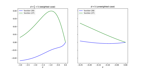
Figure 9: Plot of functions (26) and (27).

We also need an analogous lemma to Lemma D.4 for the case of $p<0$. It is easy to argue that since $x^{p}$ is now a strictly decreasing function in $x$, $\rho_{p}(S\cup A^{\prime})\geq\frac{3^{p}\cdot\left|S\right|+\sum_{v\in A^{\prime}}(d+d_{S+v}(v))^{p}}{\left|S\right|+\left|A^{\prime}\right|}$. The inequality is strict when $\left|A^{\prime}\right|<\left|A\right|$.

Proof sketch for Theorem D.5.

We are now ready to discuss the few differences in the proof of Theorem D.5 compared to the proof of Theorem 6.5. At the beginning of this section, we discussed the changes to the reduction for the case of $p<0$. We also noted that a similar argument to that in Equation 5 would hold for $p<0$, showing that $\mathsf{OPT}_{G}\leq\rho^{*}$ when the given instance $(\mathcal{S},\mathcal{U})$ contains an exact $3$-cover.

Now suppose the Exact $3$-Cover instance does not contain an exact $3$-cover. We discuss how the three cases in the proof of Theorem 6.5 would change for $p<0$. Recall that we take arbitrary sets $S\subseteq L$ and $A^{\prime}\subseteq A$ and the goal is to show that $\rho_{p}(S\cup A^{\prime})>\rho^{*}$. For case 1 (corresponding to $3\left|S\right|=\left|A^{\prime}\right|$), the only difference is that the function $\sum_{i=1}^{n}(c+x_{i})^{p}$ is convex instead of concave. The reasoning for this case still remains the same. Now we consider case 2 (corresponding to $3\left|S\right|=\beta\left|A^{\prime}\right|$ for some $\beta\in[0,1)$). There are two differences here. We first see that Lemma 6.4 holds for $p<0$, implying that $\rho_{p}(S\cup A^{\prime})$ is at least the quantity in (22). The second difference is in guaranteeing that the function in (23) is strictly decreasing in $\beta$ if and only if $3^{p}+3(d+1)^{p}<4d^{p}$. This inequality holds because of Lemma D.6 (instead of Lemma D.3).

Now we consider case 3 (corresponding to $3\left|S\right|=\alpha\left|A^{\prime}\right|$ for $\alpha>1$). There are again two differences. Lemma 6.4 holds for $p<0$, so we have that $\rho_{p}(S\cup A^{\prime})$ is at least the quantity in (24). Then we have that the function in (25) is strictly increasing in $\beta$ if $4(d+2)^{p}+3^{p}>5(d+1)^{p}$. This holds because of Lemma D.6.

D.3 Discussion on extending hardness results to all $p\in(-\infty,0)\cup(0,1)$

Weighted graphs.

Suppose one wants to prove that the weighted $p$-mean DSG is NP-hard for some $p\leq-3$. All one would have to do is define $d$ in terms of $p$ such that the inequalities in Lemma D.6 hold. For example, take $p=-10$. It would suffice to set $d=0.2p+5$ in order to prove the inequalities in Lemma D.6 hold for $p\in[-10-\delta,-10+\delta]$ for some small $\delta$. (It is important to note that this choice of $d$ would not work for $p\in[-3,-0.5]$, for example.) Once we have a definition of $d$ that allows us to prove a version of Lemma D.6 for our new choice of $p$, the proof of Theorem D.5 will still work with this new version of Lemma D.6.

Unweighted graphs.

In the unweighted case, we have less flexibility than we do for the weighted case. In this case, one potential approach to proving NP-hardness for values of $p$ in $(-\infty,-\frac{1}{8})\cup(\frac{1}{4},1)$ is to reduce from Exact $\ell$-Cover for some $\ell>3$ instead of Exact $3$-Cover and carefully choose the value of $d$, the degree of the regular graph $G[A]$. For example, the analysis goes through as above for $p=\frac{1}{2}$ if one reduces from Exact $6$-Cover and sets $d=11$. The difficulty in this approach is being able to choose a value for $d$ and $\ell$ for every given $p$.

Appendix E Experiments

E.1 Background on Frank-Wolfe

The Frank-Wolfe method is used to solve constrained convex optimization problems. Suppose we want to minimize a differentiable, convex function $f$ over a convex set $S$. The Frank-Wolfe method critically relies on the ability to efficiently optimize linear functions over $S$. The algorithm proceeds as follows. We start with an arbitrary point $x_{0}\in S$. We start iteration $k$ by first solving $y_{k}:=\operatorname*{arg\,min}_{z\in S}z^{T}\nabla f(x_{k})$. Then we let $x_{k+1}=(1-\alpha_{k})x_{k}+\alpha_{k}y_{k}$ where $\alpha_{k}$ is the step size. The standard Frank-Wolfe method sets $\alpha_{k}=\frac{2}{k+2}$.

We now discuss how we use the Frank-Wolfe method to solve $p$-mean DSG. We use the idea from [HQC22] where they take the same approach for solving $1$-mean DSG. Harb et al. introduce the following convex program for a supermodular function $f$:

$$\text{minimize }\sum_{v\in V}b_{v}^{2}\text{ subject to }b\in B_{f}$$ (28)

where

$$B_{f}=\{x\in\mathbb{R}^{V}\mid x\geq 0;x(S)\geq f(S),\forall S\subseteq V;x(V)=f(V)\}.$$

Note that $B_{f}$ is the base contrapolymatroid associated with $f$ (see, e.g., [Sch03]). [HQC22] shows that if one could obtain an optimal solution $b$ to (28), then the vertices with the largest value in $b$ will form an optimal solution to DSS (i.e. $\max_{S}\frac{f(S)}{\left|S\right|}$). We can then use the Frank-Wolfe method to obtain near-optimal solutions to (28). For rounding a near-optimal solution $b$ to (28), we use the same heuristic approach that [HQC22] and [DCS17] used for $1$-mean DSG, which is to sort the vertices in increasing order of $b$ and output the suffix with the largest density.

We address a couple of implementation aspects of using the Frank-Wolfe method to find solutions to (28). We use Frank-Wolfe to optimize over the base contrapolymatroid associated with $f_{p}$, $B_{f_{p}}$. The Frank-Wolfe method requires an initial point in the given convex set $B_{f_{p}}$. In our experiments, we start with a simple point in $B_{f_{p}}$: for all $v\in V$, we set $x_{v}=d_{G}(v)^{p}$. We experimented with other starting points, such as those based on the ordering produced by $\mathsf{Greedy\text{-}}p$, but this simple solution worked best and was much faster.

Furthermore, we note that when applying Frank-Wolfe to solve the convex program (28), the optimization problem at each iteration is essentially $\min_{z\in B_{f}}z^{T}x_{k}$ where $x_{k}$ is our current solution. We can easily solve this optimization problem as algorithms for optimizing linear functions over the base contrapolymatroid are well-understood [Lov83].

E.2 Full reporting of results

We include the full table of results in Table 4 for the experiments comparing $\mathsf{Greedy\text{-}}p$ and $\mathsf{Lazy\text{-}Greedy\text{-}}p$ on all ten real-world graphs and all values of $p\in\{1.05,1.25,1.5,1.75,2\}$. For $\mathsf{Lazy\text{-}Greedy\text{-}}p$, we report results for values of $\epsilon\in\{0.01,0.1,1\}$.

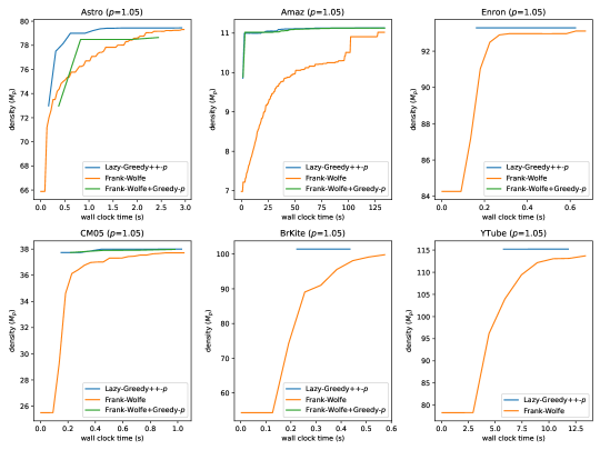
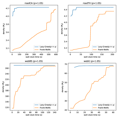
Figure 10: Experiments comparing convergence rates of the algorithms we consider in Section 7.2. Results for $p=1.05$.

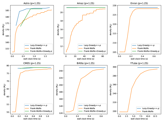
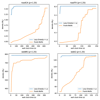
Figure 11: Experiments comparing convergence rates of the algorithms we consider in Section 7.2. Results for $p=1.25$.

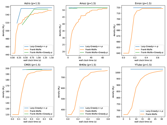
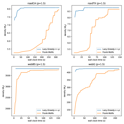
Figure 12: Experiments comparing convergence rates of the algorithms we consider in Section 7.2. Results for $p=1.5$.

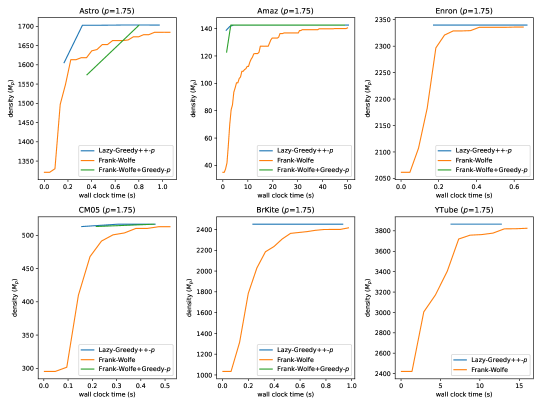
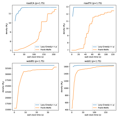
Figure 13: Experiments comparing convergence rates of the algorithms we consider in Section 7.2. Results for $p=1.75$.

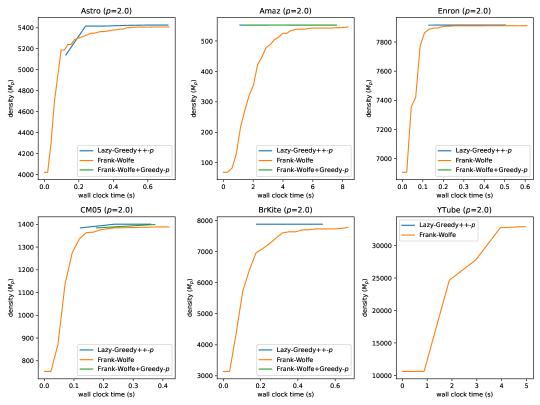
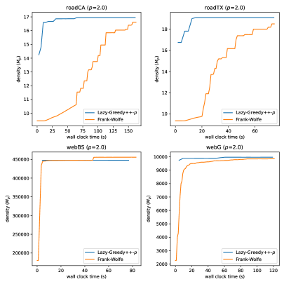
Figure 14: Experiments comparing convergence rates of the algorithms we consider in Section 7.2. Results for $p=2$.

We include results for the experiments comparing $\mathsf{Greedy}\nolinebreak[4]\raisebox{1.72218pt}{{{++}}}\text{-}p$, $\mathsf{Lazy\text{-}Greedy\nolinebreak[4]\raisebox{1.72218pt}{{{++}}}\text{-}}p$, and Frank-Wolfe on all ten real-world graphs and all values of $p\in\{1.05,1.25,1.5,1.75,2\}$. We include separate figures for each value of $p$ in Figures 10, 11, 12, 13, 14.

We include the full table of results in Table 5 for the experiments for $p$-mean DSG for $p<1$. We consider $p\in\{-1,-0.5,0.25,0.5,0.75\}$.

	metric	algorithm	Astro	CM05	BrKite	Enron	roadCA	roadTX	webG	webBS	Amaz	YTube
$p=1.05$	time (s)	$\mathsf{Lazy\text{-}G\text{-}}p$ ($\epsilon$$=$$0.01$)	0.272	0.173	0.339	0.325	3.142	2.222	23.25	32.68	1.36	15.19
		$\mathsf{Lazy\text{-}G\text{-}}p$ ($\epsilon$$=$$0.1$)	0.138	0.134	0.199	0.147	3.145	2.224	12.58	13.13	1.234	5.917
		$\mathsf{Lazy\text{-}G\text{-}}p$ ($\epsilon$$=$$1.0$)	0.103	0.107	0.148	0.109	3.191	2.227	9.521	10.07	1.041	3.886
		$\mathsf{Greedy\text{-}}p$	0.312	0.175	0.421	0.588	3.364	2.432	40.31	686.5	1.36	73.33
	density ($M_{p}$)	$\mathsf{Lazy\text{-}G\text{-}}p$ ($\epsilon$$=$$0.01$)	59.49	31.74	81.42	75.16	3.751	4.164	54.39	206.9	8.867	91.91
		$\mathsf{Lazy\text{-}G\text{-}}p$ ($\epsilon$$=$$0.1$)	59.49	31.74	81.42	75.16	3.751	4.164	54.39	206.9	8.864	91.91
		$\mathsf{Lazy\text{-}G\text{-}}p$ ($\epsilon$$=$$1.0$)	59.5	31.74	81.42	75.16	3.751	3.915	54.39	206.9	8.841	91.91
		$\mathsf{Greedy\text{-}}p$	59.49	31.74	81.42	75.16	3.751	4.007	54.39	206.9	8.867	91.91
$p=1.25$	time (s)	$\mathsf{Lazy\text{-}G\text{-}}p$ ($\epsilon$$=$$0.01$)	0.285	0.176	0.349	0.35	3.145	2.213	24.88	35.29	1.565	16.53
		$\mathsf{Lazy\text{-}G\text{-}}p$ ($\epsilon$$=$$0.1$)	0.144	0.135	0.209	0.154	3.148	2.214	13.09	13.32	1.342	7.685
		$\mathsf{Lazy\text{-}G\text{-}}p$ ($\epsilon$$=$$1.0$)	0.105	0.114	0.151	0.113	3.196	2.234	9.714	9.952	1.052	4.623
		$\mathsf{Greedy\text{-}}p$	0.312	0.174	0.424	0.581	3.146	2.284	41.85	687.2	1.38	75.98
	density ($M_{p}$)	$\mathsf{Lazy\text{-}G\text{-}}p$ ($\epsilon$$=$$0.01$)	61.6	32.7	82.7	77.21	3.756	4.054	54.63	207.4	11.46	95.5
		$\mathsf{Lazy\text{-}G\text{-}}p$ ($\epsilon$$=$$0.1$)	61.6	32.71	82.7	77.21	3.756	4.054	54.63	207.4	11.46	95.5
		$\mathsf{Lazy\text{-}G\text{-}}p$ ($\epsilon$$=$$1.0$)	61.76	32.74	82.7	77.21	3.756	3.958	54.63	207.4	11.48	95.5
		$\mathsf{Greedy\text{-}}p$	61.6	32.7	82.7	77.21	3.683	4.036	54.63	207.4	11.46	95.5
$p=1.5$	time (s)	$\mathsf{Lazy\text{-}G\text{-}}p$ ($\epsilon$$=$$0.01$)	0.294	0.174	0.36	0.329	3.151	2.215	23.99	37.91	1.365	17.34
		$\mathsf{Lazy\text{-}G\text{-}}p$ ($\epsilon$$=$$0.1$)	0.14	0.138	0.216	0.161	3.145	2.215	12.99	13.56	1.255	6.733
		$\mathsf{Lazy\text{-}G\text{-}}p$ ($\epsilon$$=$$1.0$)	0.106	0.109	0.156	0.113	3.107	2.172	9.553	9.887	1.052	4.051
		$\mathsf{Greedy\text{-}}p$	0.314	0.175	0.42	0.582	3.141	2.657	36.11	752.4	1.505	60.99
	density ($M_{p}$)	$\mathsf{Lazy\text{-}G\text{-}}p$ ($\epsilon$$=$$0.01$)	64.24	33.94	84.46	80.31	3.72	4.074	54.86	244.2	13.81	101.7
		$\mathsf{Lazy\text{-}G\text{-}}p$ ($\epsilon$$=$$0.1$)	64.32	33.94	84.46	80.31	3.72	4.074	54.86	244.2	13.81	101.7
		$\mathsf{Lazy\text{-}G\text{-}}p$ ($\epsilon$$=$$1.0$)	64.57	33.94	84.45	80.31	3.763	4.014	54.91	244.2	13.87	101.7
		$\mathsf{Greedy\text{-}}p$	64.24	33.94	84.46	80.31	3.72	4.074	54.86	244.2	13.81	101.7
$p=1.75$	time (s)	$\mathsf{Lazy\text{-}G\text{-}}p$ ($\epsilon$$=$$0.01$)	0.297	0.173	0.362	0.383	3.132	2.2	20.87	41.33	1.333	17.2
		$\mathsf{Lazy\text{-}G\text{-}}p$ ($\epsilon$$=$$0.1$)	0.157	0.141	0.223	0.176	3.135	2.198	12.28	14.16	1.245	6.931
		$\mathsf{Lazy\text{-}G\text{-}}p$ ($\epsilon$$=$$1.0$)	0.108	0.109	0.154	0.113	3.104	2.163	9.399	9.931	1.049	4.044
		$\mathsf{Greedy\text{-}}p$	0.31	0.172	0.406	0.586	3.219	2.541	31.26	742.4	1.406	68.5
	density ($M_{p}$)	$\mathsf{Lazy\text{-}G\text{-}}p$ ($\epsilon$$=$$0.01$)	67.12	35.38	86.45	84.19	3.816	4.113	66.5	387.1	15.63	112.2
		$\mathsf{Lazy\text{-}G\text{-}}p$ ($\epsilon$$=$$0.1$)	67.12	35.38	86.45	84.19	3.816	4.113	66.51	387.1	15.63	112.2
		$\mathsf{Lazy\text{-}G\text{-}}p$ ($\epsilon$$=$$1.0$)	67.88	35.37	86.44	84.19	3.769	4.071	67.68	387.1	16.76	112.2
		$\mathsf{Greedy\text{-}}p$	67.12	35.38	86.45	84.19	3.816	4.113	66.5	387.1	15.63	112.2
$p=2.0$	time (s)	$\mathsf{Lazy\text{-}G\text{-}}p$ ($\epsilon$$=$$0.01$)	0.248	0.125	0.307	0.345	2.187	1.555	18.4	41.71	0.966	16.21
		$\mathsf{Lazy\text{-}G\text{-}}p$ ($\epsilon$$=$$0.1$)	0.112	0.096	0.17	0.124	2.184	1.554	9.105	10.29	0.919	6.069
		$\mathsf{Lazy\text{-}G\text{-}}p$ ($\epsilon$$=$$1.0$)	0.057	0.064	0.101	0.066	2.161	1.528	6.089	5.217	0.748	3.272
		$\mathsf{Greedy\text{-}}p$	0.257	0.124	0.337	0.518	2.161	1.534	25.65	662.0	0.98	60.97
	density ($M_{p}$)	$\mathsf{Lazy\text{-}G\text{-}}p$ ($\epsilon$$=$$0.01$)	71.46	37.2	88.78	88.99	3.759	4.224	98.65	675.3	23.5	182.4
		$\mathsf{Lazy\text{-}G\text{-}}p$ ($\epsilon$$=$$0.1$)	71.44	37.2	88.78	88.99	3.759	4.224	99.21	675.3	23.5	182.4
		$\mathsf{Lazy\text{-}G\text{-}}p$ ($\epsilon$$=$$1.0$)	71.7	37.2	88.77	88.97	3.775	4.092	98.67	669.0	23.5	182.4
		$\mathsf{Greedy\text{-}}p$	71.46	37.2	88.78	88.99	3.759	4.224	98.65	675.3	23.5	182.4

Table 4: Results for experiments comparing $\mathsf{Greedy\text{-}}p$ to $\mathsf{Lazy\text{-}Greedy\text{-}}p$. We write $\mathsf{Lazy\text{-}Greedy\text{-}}p$ as $\mathsf{Lazy\text{-}G\text{-}}p$ for spacing issues. See Section 7.1 for more details.

	metric	algorithm	Astro	CM05	BrKite	Enron	roadCA	roadTX	webG	webBS	Amaz	YTube
$p=-1.0$	time (s)	$\mathsf{Simple\text{-}G\text{-}}p$	0.022	0.032	0.043	0.028	1.146	0.793	1.297	0.836	0.356	1.151
		1-mean DSG	2.179	2.984	4.4	2.834	164.9	111.8	117.9	76.95	37.81	117.9
		$\mathsf{Simple\text{-}G\nolinebreak[4]\raisebox{1.72218pt}{{{++}}}\text{-}}p$	2.179	2.984	4.4	2.834	164.9	111.8	117.9	76.95	37.81	117.9
	density ($M_{p}$)	$\mathsf{Simple\text{-}G\text{-}}p$	56.91	29.0	73.08	63.21	3.27	3.257	52.87	204.0	7.398	75.56
		1-mean DSG	55.52	26.64	70.28	61.19	3.583	3.833	53.99	204.0	5.45	72.8
		$\mathsf{Simple\text{-}G\nolinebreak[4]\raisebox{1.72218pt}{{{++}}}\text{-}}p$	58.92	29.0	73.08	63.21	3.75	3.833	54.17	204.0	7.398	75.56
$p=-0.5$	time (s)	$\mathsf{Simple\text{-}G\text{-}}p$	0.049	0.06	0.075	0.054	1.8	1.101	1.781	1.558	0.507	1.615
		1-mean DSG	4.649	5.505	7.566	5.26	213.7	145.4	176.7	160.7	51.3	163.9
		$\mathsf{Simple\text{-}G\nolinebreak[4]\raisebox{1.72218pt}{{{++}}}\text{-}}p$	4.649	5.505	7.566	5.26	213.7	145.4	176.7	160.7	51.3	163.9
	density ($M_{p}$)	$\mathsf{Simple\text{-}G\text{-}}p$	57.08	29.0	74.66	65.09	3.29	3.278	53.25	204.5	7.456	78.0
		1-mean DSG	57.28	27.65	72.71	63.7	3.672	3.899	54.55	204.5	5.692	75.89
		$\mathsf{Simple\text{-}G\nolinebreak[4]\raisebox{1.72218pt}{{{++}}}\text{-}}p$	59.83	29.05	74.66	65.09	3.774	3.899	54.65	204.5	7.456	78.0
$p=0.25$	time (s)	$\mathsf{Greedy\text{-}}p$	1.601	0.651	1.859	3.443	4.337	3.003	151.7	4049.2	3.08	294.0
		$\mathsf{Simple\text{-}G\text{-}}p$	0.037	0.038	0.047	0.038	0.861	0.586	1.104	1.22	0.272	0.891
		1-mean DSG	3.694	3.801	4.838	3.833	99.06	67.22	109.3	124.1	26.12	89.37
		$\mathsf{Simple\text{-}G\nolinebreak[4]\raisebox{1.72218pt}{{{++}}}\text{-}}p$	3.694	3.801	4.838	3.833	99.06	67.22	109.3	124.1	26.12	89.37
	density ($M_{p}$)	$\mathsf{Greedy\text{-}}p$	56.78	29.0	77.47	68.98	2.935	2.924	52.71	205.5	5.89	83.08
		$\mathsf{Simple\text{-}G\text{-}}p$	57.37	29.01	77.45	68.95	3.322	3.317	53.81	205.5	7.546	83.01
		1-mean DSG	60.4	29.5	76.74	68.46	3.804	4.015	55.35	205.5	6.637	82.1
		$\mathsf{Simple\text{-}G\nolinebreak[4]\raisebox{1.72218pt}{{{++}}}\text{-}}p$	61.33	30.14	77.45	68.95	3.842	4.015	55.36	205.5	7.546	83.02
$p=0.5$	time (s)	$\mathsf{Greedy\text{-}}p$	1.553	0.644	1.868	3.403	4.364	3.005	147.0	4483.8	2.792	292.3
		$\mathsf{Simple\text{-}G\text{-}}p$	0.036	0.038	0.05	0.039	0.857	0.596	1.165	1.31	0.26	0.887
		1-mean DSG	3.772	3.792	4.896	3.798	99.07	67.15	107.8	124.0	25.56	90.44
		$\mathsf{Simple\text{-}G\nolinebreak[4]\raisebox{1.72218pt}{{{++}}}\text{-}}p$	3.772	3.792	4.896	3.798	99.07	67.15	107.8	124.0	25.56	90.44
	density ($M_{p}$)	$\mathsf{Greedy\text{-}}p$	56.86	29.0	78.56	70.62	3.296	3.31	53.3	205.9	6.723	85.28
		$\mathsf{Simple\text{-}G\text{-}}p$	57.48	29.44	78.54	70.61	3.333	3.332	54.0	205.9	7.576	85.23
		1-mean DSG	61.59	30.22	78.16	70.36	3.848	4.059	55.6	205.9	7.297	84.74
		$\mathsf{Simple\text{-}G\nolinebreak[4]\raisebox{1.72218pt}{{{++}}}\text{-}}p$	61.87	30.62	78.54	70.61	3.867	4.059	55.6	205.9	7.869	85.24
$p=0.75$	time (s)	$\mathsf{Greedy\text{-}}p$	1.609	0.645	1.863	3.383	4.23	2.905	136.4	3566.4	2.751	280.2
		$\mathsf{Simple\text{-}G\text{-}}p$	0.036	0.038	0.047	0.038	0.847	0.582	1.087	1.206	0.262	0.882
		1-mean DSG	3.586	3.714	4.807	3.83	97.5	66.34	107.7	123.4	26.12	89.1
		$\mathsf{Simple\text{-}G\nolinebreak[4]\raisebox{1.72218pt}{{{++}}}\text{-}}p$	3.586	3.714	4.807	3.83	97.5	66.34	107.7	123.4	26.12	89.1
	density ($M_{p}$)	$\mathsf{Greedy\text{-}}p$	57.6	29.48	79.75	72.52	3.305	3.325	53.95	206.3	6.997	87.94
		$\mathsf{Simple\text{-}G\text{-}}p$	57.99	30.01	79.75	72.51	3.344	3.348	54.18	206.3	7.606	87.93
		1-mean DSG	62.86	31.0	79.62	72.43	3.892	4.105	55.84	206.3	8.26	87.75
		$\mathsf{Simple\text{-}G\nolinebreak[4]\raisebox{1.72218pt}{{{++}}}\text{-}}p$	62.87	31.21	79.75	72.52	3.897	4.105	55.84	206.3	8.42	87.93

Table 5: Results for algorithms for $p<1$. We write $\mathsf{Simple\text{-}Greedy\text{-}}p$ as $\mathsf{Simple\text{-}G\text{-}}p$ and $\mathsf{Simple\text{-}Greedy\nolinebreak[4]\raisebox{1.54996pt}{{{++}}}\text{-}}p$ as $\mathsf{Simple\text{-}G\nolinebreak[4]\raisebox{1.54996pt}{{{++}}}\text{-}}p$ for spacing issues. See Section 7.3 for more details.

References

- [AC09] Reid Andersen and Kumar Chellapilla. Finding dense subgraphs with size bounds. In International Workshop on Algorithms and Models for the Web-Graph, pages 25–37. Springer, 2009.
- [AITT00] Yuichi Asahiro, Kazuo Iwama, Hisao Tamaki, and Takeshi Tokuyama. Greedily finding a dense subgraph. Journal of Algorithms, 34(2):203–221, 2000.
- [AKS+14] Albert Angel, Nick Koudas, Nikos Sarkas, Divesh Srivastava, Michael Svendsen, and Srikanta Tirthapura. Dense subgraph maintenance under streaming edge weight updates for real-time story identification. The VLDB journal, 23:175–199, 2014.
- [BGM14] Bahman Bahmani, Ashish Goel, and Kamesh Munagala. Efficient primal-dual graph algorithms for MapReduce. In International Workshop on Algorithms and Models for the Web-Graph, pages 59–78. Springer, 2014.
- [BGP+20] Digvijay Boob, Yu Gao, Richard Peng, Saurabh Sawlani, Charalampos Tsourakakis, Di Wang, and Junxing Wang. Flowless: Extracting densest subgraphs without flow computations. In Proceedings of The Web Conference 2020, pages 573–583, 2020.
- [BH03] Gary D Bader and Christopher WV Hogue. An automated method for finding molecular complexes in large protein interaction networks. BMC bioinformatics, 4(1):1–27, 2003.
- [Bic12] Allan Bickle. Structural results on maximal -degenerate graphs. Discussiones Mathematicae Graph Theory, 32(4):659–676, 2012.
- [BSW19] Digvijay Boob, Saurabh Sawlani, and Di Wang. Faster width-dependent algorithm for mixed packing and covering LPs. Advances in Neural Information Processing Systems 32 (NIPS 2019), 2019.
- [Cha00] Moses Charikar. Greedy approximation algorithms for finding dense components in a graph. In International Workshop on Approximation Algorithms for Combinatorial Optimization, pages 84–95. Springer, 2000.
- [CQT22] Chandra Chekuri, Kent Quanrud, and Manuel R Torres. Densest subgraph: Supermodularity, iterative peeling, and flow. In Proceedings of the 2022 Annual ACM-SIAM Symposium on Discrete Algorithms (SODA), pages 1531–1555. SIAM, 2022.
- [DCS17] Maximilien Danisch, T.-H. Hubert Chan, and Mauro Sozio. Large scale density-friendly graph decomposition via convex programming. In Proceedings of the 26th International Conference on World Wide Web, pages 233–242, 2017.
- [DGP07] Yon Dourisboure, Filippo Geraci, and Marco Pellegrini. Extraction and classification of dense communities in the web. In Proceedings of the 16th international conference on World Wide Web, pages 461–470, 2007.
- [DH11] Timothy A Davis and Yifan Hu. The University of Florida sparse matrix collection. ACM Transactions on Mathematical Software (TOMS), 38(1):1–25, 2011.
- [DJD+09] Xiaoxi Du, Ruoming Jin, Liang Ding, Victor E Lee, and John H Thornton Jr. Migration motif: a spatial-temporal pattern mining approach for financial markets. In Proceedings of the 15th ACM SIGKDD international conference on knowledge discovery and data mining, pages 1135–1144, 2009.
- [Far08] András Faragó. A general tractable density concept for graphs. Mathematics in Computer Science, 1(4):689–699, 2008.
- [FCT14] Martin Farach-Colton and Meng-Tsung Tsai. Computing the degeneracy of large graphs. In LATIN 2014: Theoretical Informatics: 11th Latin American Symposium, Montevideo, Uruguay, March 31–April 4, 2014. Proceedings 11, pages 250–260. Springer, 2014.
- [FNBB06] Eugene Fratkin, Brian T Naughton, Douglas L Brutlag, and Serafim Batzoglou. MotifCut: regulatory motifs finding with maximum density subgraphs. Bioinformatics, 22(14):e150–e157, 2006.
- [FRM19] András Faragó and Zohre R Mojaveri. In search of the densest subgraph. Algorithms, 12(8):157, 2019.
- [GGT89] Giorgio Gallo, Michael D Grigoriadis, and Robert E Tarjan. A fast parametric maximum flow algorithm and applications. SIAM Journal on Computing, 18(1):30–55, 1989.
- [GKT05] David Gibson, Ravi Kumar, and Andrew Tomkins. Discovering large dense subgraphs in massive graphs. In Proceedings of the 31st international conference on Very large data bases, pages 721–732, 2005.
- [Gol84] Andrew V Goldberg. Finding a maximum density subgraph. University of California Berkeley, 1984.
- [GT15] Aristides Gionis and Charalampos E Tsourakakis. Dense subgraph discovery: KDD 2015 tutorial. In Proceedings of the 21th ACM SIGKDD International Conference on Knowledge Discovery and Data Mining, pages 2313–2314, 2015.
- [HQC22] Elfarouk Harb, Kent Quanrud, and Chandra Chekuri. Faster and scalable algorithms for densest subgraph and decomposition. In Advances in Neural Information Processing Systems, 2022.
- [HWC17] Shuguang Hu, Xiaowei Wu, and TH Hubert Chan. Maintaining densest subsets efficiently in evolving hypergraphs. In Proceedings of the 2017 ACM on Conference on Information and Knowledge Management, pages 929–938, 2017.
- [HYH+05] Haiyan Hu, Xifeng Yan, Yu Huang, Jiawei Han, and Xianghong Jasmine Zhou. Mining coherent dense subgraphs across massive biological networks for functional discovery. Bioinformatics, 21(suppl_1):i213–i221, 2005.
- [JZT+22] Yingsheng Ji, Zheng Zhang, Xinlei Tang, Jiachen Shen, Xi Zhang, and Guangwen Yang. Detecting cash-out users via dense subgraphs. In Proceedings of the 28th ACM SIGKDD Conference on Knowledge Discovery and Data Mining, pages 687–697, 2022.
- [KM18] Yasushi Kawase and Atsushi Miyauchi. The densest subgraph problem with a convex/concave size function. Algorithmica, 80(12):3461–3480, 2018.
- [KNT06] Ravi Kumar, Jasmine Novak, and Andrew Tomkins. Structure and evolution of online social networks. In Proceedings of the 12th ACM SIGKDD international conference on Knowledge discovery and data mining, pages 611–617, 2006.
- [Law76] E.L. Lawler. Combinatorial Optimization: Networks and Matroids. Holt, Rinehart and Winston, 1976.
- [LBG20] Tommaso Lanciano, Francesco Bonchi, and Aristides Gionis. Explainable classification of brain networks via contrast subgraphs. In Proceedings of the 26th ACM SIGKDD International Conference on Knowledge Discovery & Data Mining, pages 3308–3318, 2020.
- [LK14] Jure Leskovec and Andrej Krevl. SNAP Datasets: Stanford large network dataset collection. http://snap.stanford.edu/data, June 2014.
- [LMFB23] Tommaso Lanciano, Atsushi Miyauchi, Adriano Fazzone, and Francesco Bonchi. A survey on the densest subgraph problem and its variants. arXiv preprint arXiv:2303.14467, 2023.
- [Lov83] László Lovász. Submodular functions and convexity. In Mathematical programming the state of the art, pages 235–257. Springer, 1983.
- [LRJA10] Victor E Lee, Ning Ruan, Ruoming Jin, and Charu Aggarwal. A survey of algorithms for dense subgraph discovery. In Managing and Mining Graph Data, pages 303–336. Springer, 2010.
- [LZW+08] Zhenping Li, Shihua Zhang, Rui-Sheng Wang, Xiang-Sun Zhang, and Luonan Chen. Quantitative function for community detection. Physical review E, 77(3):036109, 2008.
- [MB83] David W Matula and Leland L Beck. Smallest-last ordering and clustering and graph coloring algorithms. Journal of the ACM (JACM), 30(3):417–427, 1983.
- [MGPV20] Fragkiskos D Malliaros, Christos Giatsidis, Apostolos N Papadopoulos, and Michalis Vazirgiannis. The core decomposition of networks: Theory, algorithms and applications. The VLDB Journal, 29:61–92, 2020.
- [MK18] Atsushi Miyauchi and Naonori Kakimura. Finding a dense subgraph with sparse cut. In Proceedings of the 27th ACM International Conference on Information and Knowledge Management, pages 547–556, 2018.
- [PQ82] Jean-Claude Picard and Maurice Queyranne. A network flow solution to some nonlinear 0-1 programming problems, with applications to graph theory. Networks, 12(2):141–159, 1982.
- [Sch03] Alexander Schrijver. Combinatorial optimization: polyhedra and efficiency, volume 24. Springer Science & Business Media, 2003.
- [SM03] Victor Spirin and Leonid A Mirny. Protein complexes and functional modules in molecular networks. Proceedings of the national Academy of sciences, 100(21):12123–12128, 2003.
- [SMT22] Issey Sukeda, Atsushi Miyauchi, and Akiko Takeda. A study on modularity density maximization: Column generation acceleration and computational complexity analysis. arXiv preprint arXiv:2206.10901, 2022.
- [TC21] Charalampos Tsourakakis and Tianyi Chen. Dense subgraph discovery: Theory and application (Tutoral at SDM 2021), 2021. https://tsourakakis.com/dense-subgraph-discovery-theory-and-applications-tutorial-sdm-2021/.
- [Tso14] Charalampos E Tsourakakis. A novel approach to finding near-cliques: The triangle-densest subgraph problem. arXiv preprint arXiv:1405.1477, 2014.
- [Tso15] Charalampos Tsourakakis. The -clique densest subgraph problem. In Proceedings of the 24th international conference on world wide web, pages 1122–1132, 2015.
- [VBK21] Nate Veldt, Austin R Benson, and Jon Kleinberg. The generalized mean densest subgraph problem. In Proceedings of the 27th ACM SIGKDD Conference on Knowledge Discovery & Data Mining, pages 1604–1614, 2021.
- [ZZY+17] Si Zhang, Dawei Zhou, Mehmet Yigit Yildirim, Scott Alcorn, Jingrui He, Hasan Davulcu, and Hanghang Tong. Hidden: hierarchical dense subgraph detection with application to financial fraud detection. In Proceedings of the 2017 SIAM International Conference on Data Mining, pages 570–578. SIAM, 2017.