Galactic Axion Laser Interferometer Leveraging Electro-Optics: GALILEO

Abstract

We propose a novel experimental method for probing light dark matter candidates. We show that an electro-optical material’s refractive index is modified in the presence of a coherently oscillating dark matter background. A high-precision resonant Michelson interferometer can be used to read out this signal. The proposed detection scheme allows for the exploration of an uncharted parameter space of dark matter candidates over a wide range of masses – including masses exceeding a few tens of microelectronvolts, which is a challenging parameter space for microwave cavity haloscopes.

The nature of dark matter (DM) in modern physics remain elusive. A well-motivated class of DM candidates is light bosonic particles. The QCD axion, for example, is a viable candidate for DM Marsh (2016); Hook (2019) in addition to solving the Strong CP problem Peccei and Quinn (1977); Weinberg (1978); Wilczek (1978). Axion-like pseudoscalar particles Marsh (2016); Hook (2019) (a generalized form of the QCD axion) and vector particles (e.g., a dark or hidden photon) Fabbrichesi et al. (2020); Caputo et al. (2021) are similarly well-motivated DM candidates. Such new particles typically have suppressed interactions with the standard model, which nevertheless can be used to search for them in the laboratory Sikivie (2021); Semertzidis and Youn (2022); Caputo et al. (2021); Adams et al. (2022); Rajendran (2022); Sushkov (2023).

Light DM is also referred to as wave-like, in contrast to heavier particle-like DM candidates. Due to the high occupancy number of such particles at galactic scales, light DM behaves as a classical wave. Such a DM background can be modeled as a classical random field $a_{0}\cos(\omega t+\mathbf{k}\cdot\mathbf{x}+\phi)$ , where $a_{0}=\sqrt{\rho_{\mathrm{DM}}}/m_{\mathrm{DM}}$ is the field amplitude given by the DM density $\rho_{\mathrm{DM}}$ and mass $m_{\mathrm{DM}}$; $|\mathbf{k}|\simeq m_{\mathrm{DM}}v$ is the wave number; and $\phi$ is a random phase. The characteristic frequency of the random field’s oscillations is given dominantly by the DM mass, with corrections from the kinetic energy, as $\omega\simeq m_{\mathrm{DM}}+m_{\mathrm{DM}}v^{2}/2$, where $v\sim 10^{-3}$ is the virial velocity in the Milky Way. The light DM field is therefore coherent over spatial separation $\lambda_{\mathrm{c}}\sim(m_{\mathrm{DM}}v)^{-1}$ and over a time scale $\tau_{\mathrm{c}}\sim(m_{\mathrm{DM}}v^{2})^{-1}$, expressed in natural Planck units Foster et al. (2021).

Several experimental programs are underway or proposed to probe the parameter space of light DM, with different methods sensitive to specific couplings to standard model physics and a particular range of DM masses. Interactions with the standard model gluons and fermions can be probed via measuring its induced oscillatory electric dipole moments (EDMs) Abel et al. (2017); Roussy et al. (2021); Schulthess et al. (2022), as well as secondary effects of an oscillatory EDM in precision experiments such as storage rings Chang et al. (2019); Pretz et al. (2020); Kim and Semertzidis (2021); Alexander et al. (2022); Karanth et al. (2022), nuclear magnetic resonance Budker et al. (2014); Aybas et al. (2021), molecular and atomic spectroscopy Graham and Rajendran (2011); Kim and Perez (2022), among others Arvanitaki et al. (2021); Berlin and Zhou (2022). Light DM candidates generically couple to electromagnetism as well, which can be investigated using high-precision methods including resonant cavity haloscopes Bartram et al. (2021); Backes et al. (2021); Kwon et al. (2021); Jeong et al. (2020); Chang et al. (2022); Melcón et al. (2020); Alesini et al. (2021); Quiskamp et al. (2022), lumped elements Salemi et al. (2021); Gramolin et al. (2021); Crisosto et al. (2020); Brouwer et al. (2022), among others Berlin et al. (2020); Ortiz et al. (2022); Romanenko et al. (2023).

Our lack of knowledge about the nature of DM makes it imperative to probe a wide range of DM parameter space. In addition, different scenarios of cosmological production of the observed DM abundance suggest a wide range of viable masses. For instance, the QCD axion is produced as the pseudo-Nambu-Goldstone boson of spontaneous breaking of the global Peccei-Quinn (PQ) symmetry Marsh (2016); Hook (2019). Importantly, the QCD axion mass that could serve as DM critically depends on whether the PQ symmetry breaks during inflation or after. Post-inflationary production of the axion serving as DM in principle predicts a unique mass. Even so, it is challenging to solve axion cosmology accurately – topological defects contribute to axion production on top of the misalignment production, making the dynamics highly nonlinear. Analytical calculations and simulations predict a post-inflationary QCD axion mass that ranges from tens to hundreds of $\mathrm{\mu eV}$ Ballesteros et al. (2017); Berkowitz et al. (2015); Bonati et al. (2016); Borsanyi et al. (2016); Dine et al. (2017); Klaer and Moore (2017); Buschmann et al. (2020), with more recent simulations suggesting a narrower range of approximately $40-180\,\mathrm{\mu eV}$ Buschmann et al. (2022). A QCD axion with even lower masses are feasible via production pre-inflation and could also serve as DM.

Resonant microwave cavity haloscopes have been the leading DM detectors for $m_{\mathrm{DM}}\sim\mathrm{\mu eV}$, achieving sensitivity to the QCD axion. However, due to the rapidly diminishing scanning rate caused by a decreasing signal-to-noise ratio (SNR) at smaller cavity volumes Adams et al. (2022), it is challenging to probe masses above a few tens of $\mathrm{\mu eV}$ with such detectors. Despite this technical limitation, ongoing efforts are being made to further optimize microwave cavity haloscopes and explore this higher-mass DM parameter space Caldwell et al. (2017); McAllister et al. (2017); Liu et al. (2022), mainly motivated by the post-inflationary axion production as discussed above.

In this Letter, we propose a new approach to detect both axion and dark photon DM over a wide mass range, approximately from $0.1-10^{3}\,\mathrm{\mu eV}$. The basic principle is as follows. Nonlinear electro-optical materials respond to the electric field induced by a coherently oscillating light DM background: the material’s refractive index thereby acquires oscillatory corrections. We outline a resonant readout scheme based on laser interferometry to detect such DM-induced signals (Fig. 1). A Michelson interferometer using a nonlinear electro-optical material in only one arm will exhibit an oscillatory differential optical phase between its two arms, imprinted in the measured interferometry fringes. We refer to this experimental approach as GALILEO: Galactic Axion Laser Interferometer Leveraging Electro-Optics. In the following, we present projected sensitivities for this measurement scheme for both the axion and dark photon DM parameter spaces, and compare to the current state of the art (Fig. 2). Note that for the light DM mass range considered here, the induced oscillations in material refractive index and hence interferometer output signal are in a frequency range $\sim$ 100 MHz to 1 THz; and the light-DM background field is coherent over $\mathrm{\lambda_{c}\sim}$ 1 cm to 100 m and $\mathrm{\tau_{c}\sim 0.1\,\mu s}$ to ms.

Electro-optic effect.—

Light-DM-induced electric fields can be detected via interactions that modulate an electro-optical (EO) material’s properties. In particular, the presence of an external electric field results in a change in the polarization of the material, which then modifies the dispersion relation of the electromagnetic wave inside the material. Therefore, one can detect ambient electric fields, such as that induced by light DM, by measuring the effect on propagation of a probe laser through an EO material Xue et al. (2022).

This scheme requires a nonlinear response of the material that couples the probe laser and the light-DM-induced electric field to be sensed, $E_{\mathrm{DM}}$. This property can be found in electro-optical materials, where the polarization is given by $P=\epsilon_{0}\chi^{(1)}E+\epsilon_{0}\chi^{(2)}E^{2}+\mathcal{O}(E^{3})$ Powers and Haus (2017). Here, $\epsilon_{0}$ is the vacuum permittivity and $\chi^{(n)}$ is the $n$-th order electric susceptibility of the material . We define an effective electric susceptibility as follows: $\chi_{\mathrm{eff.}}=\chi^{(1)}+\delta\chi$, where $\delta\chi=\chi^{(2)}E_{\mathrm{DM}}$. Since the effect of DM is expected to be small, one can treat the additional term $\delta\chi$ perturbatively. The electric susceptibility $\chi_{\mathrm{eff.}}$ is used to calculate a medium’s refractive index via $n=(1+\chi_{\mathrm{eff.}})^{1/2}$. Therefore, in the presence of non-zero $E_{\mathrm{DM}}$ we have a correction to the material’s refractive index proportional to the light-DM-induced electric field $n=\bar{n}+\delta n$, where $\delta n\simeq\delta\chi/2\bar{n}$. We calculate this DM-induced refractive index correction for a given set of DM parameters and material properties.

Electro-optic properties due to $\chi^{(2)}$ (i.e., the Pockels effect) can be observed in crystals lacking inversion symmetry. These materials are typically used for applications that employ modulations of the refractive index to achieve fast optical switching and frequency conversion. A widely used example of such a crystal is lithium niobate ($\mathrm{LiNbO_{3}}$) Weis and Gaylord (1985); Vazimali and Fathpour (2022), while barium titanate ($\mathrm{BaTiO_{3}}$) is an emerging material with a higher Pockels coefficient Abel et al. (2019); Eltes et al. (2019). We use these two crystals as benchmarks for the light-DM detector material in our interferometry measurement scheme. The Pockels coefficient $r$ is defined such that the modulation in the refractive index due to an applied electric field is $\delta n=\bar{n}^{3}rE/2$. Note that $r$ is a tensor quantity, with its largest component being about $31\,\mathrm{pm/V}$ Weis and Gaylord (1985) ($923\,\mathrm{pm/V}$ Abel et al. (2019)) for $\mathrm{LiNbO_{3}}$ ($\mathrm{BaTiO_{3}}$). Therefore, we have:

$$\delta n\sim\begin{cases}1.8\times 10^{-10}\,(\mathrm{m/V})~{}E_{\mathrm{DM}},&\text{for $\mathrm{LiNbO_{3}}$}\\ 6.4\times 10^{-9}\,(\mathrm{m/V})~{}E_{\mathrm{DM}},&\text{for $\mathrm{BaTiO_{3}}$}\end{cases}$$ (1)

where we used $\bar{n}=2.3$ for $\mathrm{LiNbO_{3}}$ and $\bar{n}=2.4$ for $\mathrm{BaTiO_{3}}$.

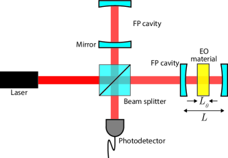
Figure 1: Schematic of the proposed laser interferometer-based light dark matter (DM) detector, GALILEO. The Fabry-Perot (FP) cavities are resonant with the light-DM mass $L=2n\pi/m_{\mathrm{DM}}$. The electro-optical (EO) material’s thickness is limited to $L_{0}\leq\pi/m_{\mathrm{DM}}$ to preserve the oscillatory DM signal while averaging over laser travel time through the material. Note that the EO material needs to be exposed to a large, uniform magnetic field for axion-induced effects. See text for details.

Dark matter-induced electric field.—

We first consider axion DM coupling to photons:

$$\mathcal{L}\supset-\dfrac{g_{a\gamma\gamma}}{4}aF_{\mu\nu}\tilde{F}^{\mu\nu}=g_{a\gamma\gamma}a\mathbf{E}\cdot\mathbf{B}$$ (2)

where $a$ and $F$ are the pseudoscalar axion field and electromagnetic field strength, respectively. This interaction modifies Maxwell’s equations. In particular, the axion field generate oscillatory electric and magnetic fields in the presence of a large bias magnetic field $B_{0}$. When the Compton wavelength of the axion $2\pi/m_{\mathrm{a}}$ is smaller than the physical size of the magnet, the axion-induced electric field is given by $E_{\rm a}\sim g_{a\gamma\gamma}aB_{0}$ Beutter et al. (2019); Ouellet and Bogorad (2019). Therefore, we have:

$$E_{\rm a} \simeq 5.6\times 10^{-9}\,{\rm\dfrac{V}{m}}\left(\dfrac{g_{a\gamma\gamma}}{10^{-10}\,{\rm GeV}^{-1}}\right)\left(\dfrac{\rho_{\odot}}{0.45\,\rm{GeV}/{\rm cm}^{3}}\right)^{1/2}$$

$$\quad\times\left(\dfrac{m_{a}}{100\,{\rm\mu eV}}\right)^{-1}\left(\dfrac{B}{10\,{\rm T}}\right)$$ (3)

For dark photon DM, we consider the kinetic mixing Lagrangian term:

$$\mathcal{L}\supset-\dfrac{\kappa}{2}F_{\mu\nu}F^{\prime\mu\nu}$$ (4)

where $\kappa$ is the dimensionless mixing parameter and $F^{\prime}$ is the dark photon field strength. The light-DM-induced electric field due to this mixing term is $E_{\rm d.p.}\sim\kappa\sqrt{\rho_{\odot}/\epsilon_{0}}$. Therefore, we have:

$$E_{\rm d.p.}\simeq 2.8\times 10^{-8}\,{\rm\dfrac{V}{m}}\left(\dfrac{\kappa}{10^{-11}}\right)\left(\dfrac{\rho_{\odot}}{0.45\,\rm{GeV}/{\rm cm}^{3}}\right)^{1/2}$$ (5)

Detection scheme.—

We propose using an asymmetric Michelson interferometer, where the sensing volume of the EO material is placed in one arm but not in the other; see Fig. 1. Due to the modulated refractive index, the probe laser will experience a modulated phase velocity as it propagates through the EO material according to $\delta v=-\delta n/\bar{n}^{2}$. The differential phase velocity between the two arms, integrated over the length of the material, leads to an effective differential arm length $\delta L=\int\mathrm{d}t\,\delta v=-\delta nL_{0}/\bar{n}$. Hence, the interferometer output will oscillate with the light-DM oscillation frequency.

Interferometer arms can be equipped with a Fabry-Perot (FP) cavity to further increase the sensitivity via increasing the effective integration length as $L_{\mathrm{eff}}=L_{0}N\mathcal{F}$, where $L_{0}$, $N$, and $\mathcal{F}$ are the EO material’s thickness, number of EO material pieces in the cavity, and finesse of the FP cavity. In order to not average over DM oscillations as the laser beam travels through an EO material of thickness $L_{0}$, we require that $L_{0}\leq\pi/m_{\mathrm{DM}}$, in natural Planck units. Ultra-high-finesse FP cavities with $\mathcal{F}\sim 1.5\times 10^{5}$ are developed for precision experiments Muller et al. (2010); Pugla (2008); Nicolodi et al. (2018). We also note that FP cavities achieve Q-factors $\gg 10^{6}$ via extending the cavity length, despite a lower finesse De Riva et al. (1996). Therefore, it is feasible to include multiple EO materials separated by $2\pi/m_{\mathrm{DM}}$ in a single cavity. The effective travel length through the total amount of EO material is ultimately limited by laser absorption. Absorption coefficient for pure, high-Q nonlinear crystals (including $\mathrm{LiNbO_{3}}$ Leidinger et al. (2015)) is about $10^{-5}\mathrm{cm^{-1}}$, i.e., $\mathcal{O}(1)$ fraction of the laser power gets absorbed after about $1\,\mathrm{km}$ of traversing inside the EO material. Therefore, we set an upper limit on $L_{\mathrm{eff}}\leq 1\,\mathrm{km}$.

Before moving on to computing signal-to-noise (SNR) values for this measurement scheme, we provide the transfer function that relates the light-DM-induced modulation of the refractive index (1) to the interferometer output signal power:

$$\dfrac{\delta P_{\rm out}}{\delta n}=\dfrac{\delta P_{\rm out}}{\delta L}\dfrac{\delta L}{\delta n}=\dfrac{2\pi}{\lambda\bar{n}}P_{\rm in}L_{0}N\mathcal{F}$$ (6)

where, we used $\delta P_{\rm out}/\delta L=(2\pi/\lambda)P_{\rm in}N\mathcal{F}\sin(8\pi\Delta L/\lambda)$ in the second equality Cahillane (2021). Here, $\lambda$ is the laser wavelength and $\Delta L$ is a DC offset between the two arm lengths, which we choose such that $\delta P_{\rm out}/\delta L$ is maximum, thereby giving optimal sensitivity to a light DM background.

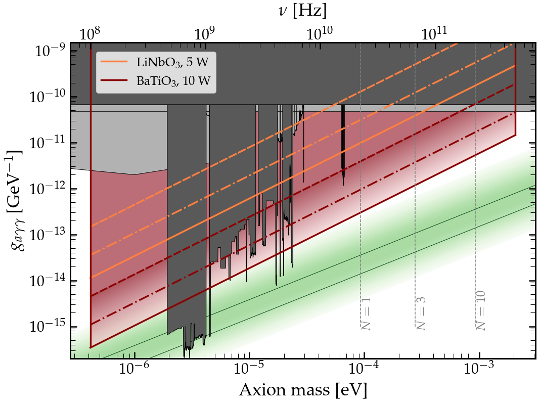
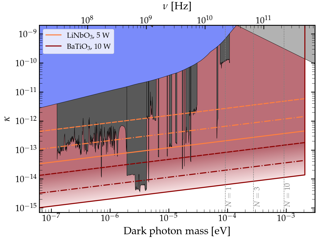
Figure 2: Projected sensitivities of the GALILEO experiment for axion (Left) and dark photon (Right) dark matter searches. The red shaded area is within the reach of the proposed detector. Orange (red) lines: $\mathrm{LiNbO_{3}}$ ($\mathrm{BaTiO_{3}}$) as target electro-optical material. Dashed lines: 1 s averaging at each frequency band $\Delta f=m_{\mathrm{DM}}/(2\pi\mathcal{F})$. Dash-dotted lines: extended search time of $290$ s per bin, equivalent to scanning a decade in mass for about 3 years. Solid lines: $290$ s averaging time per bin and 10 dB squeezing of light input to the interferometer. Vertical gray dashed lines indicate the number of EO material pieces $N=1,3,$ and $10$ needed to achieve maximum sensitivity at representative DM masses if each EO material has a thickness of $L_{0}=\pi/m_{\mathrm{DM}}$. See text for details. Dark (light) gray shaded areas are excluded by terrestrial experiments (astrophysical observations). Green: QCD axion parameter space. Blue: excluded by dark photon DM cosmology Arias et al. (2012). Existing limits are adapted from ref. O’Hare (2020).

Experimental feasibility and projected sensitivities.—

Quantum noise and thermal noise are the fundamental sources of noise in the described interferometer measurement scheme. Here, we estimate these two noise sources and show that the proposed experiment can reach the quantum noise limit for experimentally feasible parameters. Technical noise mitigation (such as laser frequency and phase noise) is also an important aspect of the final detector, which can benefit from well-established techniques used in state-of-the-art high-precision laser interferometers like LIGO Abbott et al. (2016); Cahillane et al. (2021); Cahillane and Mansell (2022). We leave a detailed description of the detector design for a follow-up study. We next discuss the sources of quantum and thermal noise.

Photon counting (shot) noise is the fundamental quantum-mechanical limit of a laser interferometer Caves (1981). The number of detected photons follows Poissonian counting statistics, which leads to an output power uncertainty of $\delta P_{\mathrm{out}}=\hbar\omega_{\mathrm{L}}\sqrt{N_{\mathrm{out}}}/\tau$, where $\omega_{\mathrm{L}}$ is the carrier photon frequency and $N_{\mathrm{out}}$ is the number of detected photons in the output port over integration time $\tau$. The shot noise amplitude spectral density (ASD) is $\delta P_{\mathrm{out}}/\sqrt{\Delta f}$, with $\Delta f$ being the bandwidth, which can thus be expressed as:

$$\mathrm{ASD_{s.n.}}=\sqrt{2\hbar\omega_{\mathrm{L}}P_{\mathrm{out}}}=\sqrt{\hbar\omega_{\mathrm{L}}P_{\mathrm{in}}}\,.$$ (7)

The second fundamental noise source is thermal noise, which has been extensively studied in the context of gravitational wave laser interferometers Levin (1998); Braginsky et al. (1999, 2000); Evans et al. (2008); Dwyer and Ballmer (2014). There are several mechanisms that contribute to the total thermal noise. Homogeneous damping within a material, which is characterized by the imaginary component of Young’s modulus, induces interferometer phase noise through elastic deformations of the material. In the presence of inhomogeneous/space-dependent temperature variations, heat flow leads to entropy redistribution and therefore energy dissipation and thermal noise. Such temperature variations can arise from temporal, stochastic fluctuations at a finite temperature or from the photo-thermal effect, i.e., photon absorption inside the material. These fluctuations induce interferometer phase noise via the thermo-elastic effect (due to a non-zero thermal expansion coefficient) and the thermo-refractive effect (due to a non-zero refractive index). In the Supplemental Material, each of the noise sources is estimated using the fluctuation-dissipation theorem (FDT); we find that photon shot noise dominates over thermal noise for temperatures around 200 K and below. This operational temperature can be achieved even with a few watts of laser absorption (and therefore heat generation) via active cooling feedback Shapiro et al. (2017).

In order to project the sensitivity of the GALILEO experiment in the light-DM parameter space, we calculate the shot noise-limited and time-averaged SNR. The DM coherence time $\tau_{\mathrm{c}}$ plays an important role here. As long as the integration time $t<\tau_{\mathrm{c}}$, the total number of interferometer signal photons scales linearly with t, the shot noise scales as $\sqrt{t}$, and hence the measurement $\mathrm{SNR\propto\sqrt{t}}$. The SNR degrades for $t>\tau_{\mathrm{c}}$ as the phase of the light-DM background field varies during the measurement. However, the overall measurement sensitivity to the presence of a non-zero average light-DM background field can still be improved with repeated independent measurements, each lasting for time $\mathrm{\tau_{c}}$, with the resulting SNR scaling as $\sqrt{T/\tau_{\mathrm{c}}}$, where $T$ is the total overall time of the repeated measurements. In this repeated measurement regime, the effective noise power spectral density scales as $(T/\tau_{\mathrm{c}})^{-1/2}$. The SNR scaling behavior in the two regimes can be combined as Budker et al. (2014):

$${\rm SNR}=\dfrac{\rm\delta P_{\mathrm{out}}}{\mathrm{ASD_{s.n.}}}(\tau_{\mathrm{c}}T)^{1/4}$$ (8)

Using Eqs. (1), (6), and (7), we thus estimate GALILEO SNR values for axion and dark photon DM as follows:

$${\rm SNR}\simeq\left(\dfrac{L_{0}N\mathcal{F}}{6.7\,\mathrm{mm}\times 1.5\times 10^{5}}\right)\left(\dfrac{\lambda}{1064\,\mathrm{nm}}\right)^{-1/2}\left(\dfrac{P_{\rm in}}{5\,{\rm W}}\right)^{1/2}\left(\dfrac{T}{\mathrm{s}}\right)^{1/4}\times\begin{cases}20\left(\dfrac{g_{a\gamma\gamma}}{10^{-10}\,\mathrm{GeV}^{-1}}\right)\left(\dfrac{B}{10\,{\rm T}}\right)\left(\dfrac{m_{\rm DM}}{100\,\mathrm{\mu eV}}\right)^{-5/4}\\ 120\left(\dfrac{\kappa}{10^{-11}}\right)\left(\dfrac{m_{\rm DM}}{100\,\mathrm{\mu eV}}\right)^{-1/4}\end{cases}$$ (9)

where we use $\mathrm{BaTiO_{3}}$ as the EO material. We set projections in the axion and dark photon DM parameter space using the criterion $\mathrm{SNR\sim 1}$, as shown in Fig. 2.

To achieve maximum sensitivity in the higher-mass regime, we propose using multiple EO materials inside a FP cavity, each separated by $2\pi/m_{\mathrm{DM}}$. As discussed above, laser absorption in the EO material limits $L_{\mathrm{eff}}\leq\mathrm{1\,km}$. This means that for $\mathcal{F}=1.5\times 10^{5}$ we have $L_{0}N\lesssim\mathrm{6.7\,mm}$. Therefore, for $m_{\mathrm{DM}}\lesssim\mathrm{90\,\mu eV}$ (corresponding to $L_{0}\gtrsim\mathrm{6.7\,mm}$) we use a single EO material with a thickness of $\mathrm{6.7\,mm}$; whereas for $m_{\mathrm{DM}}\gtrsim\mathrm{90\,\mu eV}$ (corresponding to $L_{0}=\pi/m_{\mathrm{DM}}<\mathrm{6.7\,mm}$) we use multiple EO materials. Vertical gray dashed lines in Fig. 2 indicate the required number of EO materials for the higher-mass DM parameter space to achieve maximum sensitivity.

In the proposed detection scheme, the background DM-induced electric field oscillations manifest as an oscillatory signal at the interferometer output. It is therefore crucial to have a high photodetector bandwidth in order to resolve higher-mass DM-induced oscillations. While commercially available low-noise photodetectors have a bandwidth of up to 50 GHz (corresponding to $m_{\mathrm{DM}}\simeq\mathrm{210\,\mu eV}$), there are currently demonstrations of detectors with bandwidths up to 500 GHz Yin et al. (2018); Lischke et al. (2021). The EO material’s response time will also limit detection of DM masses higher than a few $\mathrm{meV}$. We thus set a higher mass limit of about 2 meV in Fig. 2, corresponding to a photodetector bandwidth of about 500 GHz. In the low-mass axion regime the Fabry-Perot cavity length becomes a limiting factor, because at least one arm of the interferometer must be within the magnet producing the large bias magnetic field necessary for axion-induced signals. Therefore, we consider only axion masses greater than $\mathrm{0.4\,\mu eV}$ in the sensitivity estimations. This requirement is more relaxed for dark photon searches, where no background magnetic field is needed.

It is possible to reduce the observed noise below the nominal shot-noise limit through squeezing, where the electromagnetic vacuum noise in the measurement readout quadrature is reduced, with a corresponding increase of the noise in the other quadrature, consistent with the Heisenberg quantum limit. To date, laser interferometric gravitational wave detectors have successfully achieved 10 dB vacuum squeezing Vahlbruch et al. (2008); Zander et al. (2023); Tse et al. (2019), which is equivalent to improved sensitivity by a factor of about 3. As part of our sensitivity projections in Fig. 2, we also consider squeezing to further improve the detector reach.

Summary.—

We proposed a new approach to detect axion and dark photon dark matter (DM) over almost four decades in mass from about $0.1-10^{3}\,\mathrm{\mu eV}$. We dub this experiment GALILEO, which is based on laser interferometry and uses electro-optical properties to detect DM-induced electric fields. The proposed experiment explores parameter spaces that are challenging to probe with resonant cavity haloscopes in the high mass and low mass regimes. Future technical improvements, such as the development of materials with enhanced electro-optical properties, may extend the reach of this approach to the QCD axion dark matter parameter space across a range of several orders of magnitude for the axion mass.

We are grateful to John W. Blanchard, Johannes Cremer, Anson Hook, Jner Tzern (JJ) Oon, Aakash Ravi, and Erwin H. Tanin for insightful discussions. This work was supported by the Argonne National Laboratory under Award No. 2F60042; the Army Research Laboratory MAQP program under Contract No. W911NF-19–2-0181; the DOE fusion program under Award No. DE-SC0021654; and the University of Maryland Quantum Technology Center. This work was also supported by the U.S. Department of Energy (DOE), Office of Science, National Quantum Information Science Research Centers, Superconducting Quantum Materials and Systems Center (SQMS) under contract No. DE-AC02-07CH11359. D.E.K. and S.R. are supported in part by the U.S. National Science Foundation (NSF) under Grant No. PHY-1818899. S.R. is also supported by the DOE under a QuantISED grant for MAGIS, and the Simons Investigator Award No. 827042.

Supporting information regarding thermal noise sources is provided in this Supplemental Material.

I Thermal noise sources

The fluctuation-dissipation theorem (FDT) allows thermal noise contributions to a GALILEO measurement to be characterized according to the associated loss mechanism. Before estimating various noise contributions, let us briefly review the FDT. The temperature-dependent fluctuations of the effective interferometer arm length difference (i.e., effective displacement) $z$ as our observable can be written as:

$$\delta z=\mathcal{A}\int\mathrm{d}^{3}\mathbf{r}~{}\delta T(\mathbf{r})q(\mathbf{r})$$ (1)

where $q(\mathbf{r})$ is a space-dependent form factor and $\mathcal{A}$ is a coefficient that relates temperature to the observable of interest $z$. In this work, the form factor is proportional to the laser beam intensity profile in the transverse plane and is assumed constant along the beam line, i.e.,

$$q(\mathbf{r})\propto I(x,y)=\dfrac{1}{\pi R_{\rm beam}^{2}}e^{-(x^{2}+y^{2})/R_{\rm beam}^{2}}\,.$$ (2)

with $R_{\rm beam}$ being the Gaussian width of the optical beam intensity profile.

We are interested in calculating the noise power spectral density (PSD) $S_{\delta z}=\langle\delta z(\omega)\delta z^{\ast}(\omega)\rangle$ where $\omega$ is an arbitrary frequency within the range of light-DM masses relevant for the detector. According to FDT, one performs the following steps for each relevant loss mechanism:

• Assume a periodic, local entropy injection $\delta s_{\rm inj}(r)$ to the measurement system, with a density of

  $$\dfrac{\delta s_{\rm inj}(\mathbf{r})}{\delta V}=\dfrac{1}{T}\dfrac{\delta Q_{\rm inj}(\mathbf{r})}{\delta V}=F_{0}\cos(\omega t)q(\mathbf{r})$$ (3)

  where $\delta Q_{\rm inj}$ is the injected heat/energy, and $T$ is the mean temperature. If $z$ has dimensions of length, then $F_{0}$ has dimensions of force, with a magnitude set by the specific loss mechanism being considered.

• Calculate the dissipated power $W_{\rm diss}$ associated with each loss mechanism considered.

• Compute the the noise PSD for each loss mechanism via

  $$S_{\delta z}(\omega)=\mathcal{A}^{2}\dfrac{8k_{B}T}{\omega^{2}}\dfrac{\langle W_{\rm diss}\rangle}{F_{0}^{2}}$$ (4)

  where $k_{B}$ is the Boltzmann constant and $\langle\cdots\rangle$ denotes time-averaging over one cycle with period $2\pi/\omega$.

Parameter	Value	Description
$\mathcal{F}$	$\sim 10^{5}$	Cavity finesse
$P$	$5\,\mathrm{W}$	Laser power
$\lambda$	$1064\,\mathrm{nm}$	Laser wavelength
$R_{\rm beam}$	$1\,\mathrm{cm}$	Gaussian width of the laser beam
$T$	$200\,\mathrm{K}$	Cavity temperature
$L_{z}$	$L_{0}\leq 6.7\,\mathrm{mm}$	EO material thickness
$L_{x,y}$	$5\,\mathrm{cm}$	EO material lateral dimensions
$\sigma$	$0.25$	Poisson ratio∗
$Y_{\rm 0}$	$170\,\rm{GPa}$	Young’s modulus∗
$\varphi$	$10^{-6}$	Loss angle∗
$\rho$	$4.64\,\mathrm{g/cm^{3}}$	Density∗
$\kappa$	$4.6\,\mathrm{W/(m\cdot K)}$	Thermal conductivity∗
$C$	$628\,\mathrm{J/(kg\cdot K)}$	Heat capacity∗
$\alpha$	$\mathrm{14.8\times 10^{-6}/K}$	Thermal expansion∗
$\beta$	$\sim 5\times 10^{-4}/\mathrm{K}$	Thermo-refractive coefficient∗
∗The material properties are reported for $\mathrm{LiNbO_{3}}$.

Table 1: Benchmark experimental parameters.

Table 1 provides benchmark experimental parameters. Note that we choose the hierarchy $L_{z}<R_{\rm beam}\ll L_{x,y}$, which is analogous to the geometry of LIGO mirror coatings; the calculations that follow will also be analogous.

We will compare different thermal noise contributions with quantum (photon shot) noise, assuming lithium niobate ($\mathrm{LiNbO_{3}}$) as the electro-optic (EO) material, with the amplitude spectral density (ASD) of the quantum noise (see the main text for details):

$$\mathrm{ASD_{s.n.}}=\sqrt{\hbar\omega_{\mathrm{laser}}P_{\mathrm{in}}}=9.7\times 10^{-10}\,\mathrm{\dfrac{W}{\sqrt{Hz}}}\,.$$ (5)

Using the transfer function $\delta P_{\rm out}/\delta L=(2\pi/\lambda)P_{\rm in}N\mathcal{F}\sim 2\times 10^{13}\,\mathrm{W/m}$ we can translate this ASD to an effective displacement ASD:

$$\mathrm{ASD_{s.n.}}=\sqrt{\mathcal{S}_{\delta z}}\sim 4\times 10^{-23}\,\mathrm{\dfrac{m}{\sqrt{Hz}}}$$ (6)

According to the following computations of the thermal noise sources for an operational instrument temperature $\mathrm{<200\,K}$, we conclude that in the DM mass range of interest:

$$\mathrm{ASD_{thermal}<ASD_{s.n.}}$$ (7)

I.1 Brownian noise

Homogeneous mechanical damping inside a material is typically characterized by an imaginary contribution to the Young’s modulus:

$$Y=Y_{0}[1+i\varphi(\omega)]$$ (8)

where $\varphi$ is the so-called loss angle, which is given by the quality factor of the material’s internal mechanical modes as $\varphi=1/Q_{\rm int}$. The dissipated power due to $\varphi$ can be written as $\left\langle W_{\rm diss|mechanical}\right\rangle=\omega\varphi(\omega)U_{\rm def}$, where $U_{\rm def}$ is the maximum elastic deformation energy of the material under an oscillatory drive at frequency $\omega$. Assuming that $L_{x,y}\gg R_{\rm beam}$ and that the mechanical resonance frequencies are far away from $\omega$, one recovers the well-known result for the Brownian noise PSD as studied in the context of interferometric gravitational wave detectors Levin (1998):

$$S_{\delta z|\mathrm{Brownian}}\simeq 1.87\times\dfrac{8k_{B}T}{\omega}\dfrac{1-\sigma^{2}}{\pi^{2}Y_{0}R_{\rm beam}}\varphi$$ (9)

where the numerical factor $1.87$ applies to a Gaussian optical beam. Therefore, for $\mathrm{LiNbO_{3}}$ EO material in the GALILEO detector we have:

$$\rm{ASD}_{\rm Brownian}=\sqrt{S_{\delta z|\mathrm{Brownian}}}\simeq 6.1\times 10^{-24}\left(\dfrac{2\pi\times 10\,\mathrm{GHz}}{\omega}\right)^{1/2}\,\dfrac{\mathrm{m}}{\sqrt{\mathrm{Hz}}}$$ (10)

for the choice of parameters in Table 1.

I.2 Inhomogeneous thermal noise

Whenever there is space-dependent temperature variations $\delta T(\mathbf{r})$, there will be entropy redistribution, and therefore dissipation, due to heat flow. The rate of change of entropy density $s$ in terms of heat flow per unit area $\mathbf{j}$ is given by $\dot{s}=-({\nabla}\cdot\mathbf{j})/T$, which implies:

$$W_{\rm diss}=-T\int\mathrm{d}^{3}\mathbf{r}\dfrac{{\nabla}\cdot\mathbf{j}}{T}=\underbrace{-T\int\mathrm{d}^{2}\vec{A}\cdot\dfrac{\mathbf{j}}{T}}_{\rm surface}\underbrace{-T\int\mathrm{d}^{3}\mathbf{r}~{}\mathbf{j}\cdot\nabla(\dfrac{1}{T})}_{\rm bulk}$$ (11)

where we used $W_{\rm diss}=T\dot{S}$. Using $\kappa$ as the thermal conductivity in the bulk, i.e., $\mathbf{j}=-\kappa\nabla T$, the second term can be written as:

$$W_{\rm diss|bulk}=\dfrac{\kappa}{T}\int\mathrm{d}^{3}\mathbf{r}~{}(\nabla\delta T)^{2}$$ (12)

To proceed with the surface term, we assume radiative thermal equilibrium with the surrounding environment, which implies a vanishing net radiative heat flow. However, at first order we have $\mathbf{j}=4\epsilon_{\rm emm}\sigma_{\rm SB}T^{3}\delta T$ (linearized Stefan-Boltzmann law), where $\epsilon_{\rm emm}$ and $\sigma_{\rm SB}$ are the EO material’s emissivity and Stefan-Boltzmann constant, respectively. As a result, the radiative surface dissipation is:

$$W_{\rm diss|surface}=\dfrac{1}{T}\int\mathrm{d}^{2}\vec{A}\cdot\mathbf{j}\delta T=4\epsilon_{\rm emm}\sigma_{\rm SB}T^{2}\int\mathrm{d}x\mathrm{d}y~{}\delta T^{2}$$ (13)

Next, we employ the process of entropy injection according to Eq. (3), so that we can use the FDT to compute the noise PSD. We solve the diffusion equation with this source:

$$\rho C\dot{\delta T}-\kappa\nabla^{2}\delta T=\partial_{t}\left(\dfrac{\partial Q_{\rm inj}}{\partial V}\right)$$ (14)

which can be greatly simplified considering the hierarchy of length scales involved in the problem. We notice that the sharpest spatial heat injection gradient in the system is given by the laser beam radius. For the benchmark parameters given in Table 1, we can thus neglect the second term in the diffusion equation. As a result,

$$\delta T=\dfrac{1}{\rho C}TF_{0}\cos(\omega t)q(\mathbf{r})$$ (15)

with $q(\mathbf{r})=(1/L_{z})I(x,y)$. The bulk and surface dissipated power, following the above integrals, are Dwyer and Ballmer (2014):

$$\left\langle W_{\rm diss|bulk}\right\rangle= \dfrac{\kappa TF_{0}^{2}}{2\rho^{2}C^{2}}\dfrac{1}{L_{z}}\dfrac{1}{\pi R_{\rm beam}^{4}}$$ (16)

$$\left\langle W_{\rm diss|surface}\right\rangle= \dfrac{2\epsilon_{\rm emm}\sigma_{\rm SB}T^{4}F_{0}^{2}}{\rho^{2}C^{2}}\dfrac{1}{L_{z}^{2}}\dfrac{1}{\pi R_{\rm beam}^{2}}$$ (17)

Thermo-elastic effect.

Temperature fluctuations can couple to the interferometer phase noise through thermal expansion Braginsky et al. (1999). For a non-zero thermal expansion coefficient $\alpha\neq 0$,

$$\delta z\equiv\delta L_{z}=\alpha(1+\sigma)L_{z}\delta T$$ (18)

where, $\sigma$ is the Poisson ratio. Therefore, the $\mathcal{A}$ coefficient in the FDT for thermo-elastic noise source is:

$$\mathcal{A}_{\rm TE}=\alpha(1+\sigma)L_{z}$$ (19)

Thermo-refractive effect.

Temperature fluctuations can also couple to the interferometer phase noise through the temperature dependence of the refractive index Braginsky et al. (2000). In other words, if $\beta=\mathrm{d}n/\mathrm{d}T\neq 0$,

$$\delta z\equiv\delta L_{z}=-\beta\lambda\delta T$$ (20)

In this case, the corresponding $\mathcal{A}$ coefficient is:

$$\mathcal{A}_{\rm TR}=-\beta\lambda$$ (21)

As pointed out in Evans et al. (2008), we should consider thermo-elastic and thermo-refractive effects coherently. We thus define a total coefficient:

$$\mathcal{A}=\mathcal{A}_{TE}+\mathcal{A}_{TR}=\alpha(1+\sigma)L_{z}-\beta\lambda$$ (22)

Finally, we are ready to combine all results into the FDT, and compute the bulk and surface contributions to the interferometer noise:

$$S_{\rm\delta z|bulk}= \mathcal{A}^{2}\dfrac{4k_{B}\kappa}{\omega^{2}}\dfrac{T^{2}}{\rho^{2}C^{2}}\dfrac{1}{L_{z}}\dfrac{1}{\pi R_{\rm beam}^{4}}$$ (23)

$$S_{\rm\delta z|surface}= \mathcal{A}^{2}\dfrac{16k_{B}\epsilon_{\rm emm}\sigma_{\rm SB}}{\omega^{2}}\dfrac{T^{5}}{\rho^{2}C^{2}}\dfrac{1}{L_{z}^{2}}\dfrac{1}{\pi R_{\rm beam}^{2}}$$ (24)

which implies,

$$\rm{ASD}_{\rm bulk}=\sqrt{S_{\rm\delta z|bulk}}= 5.6\times 10^{-29}\left(\dfrac{2\pi\times 10\,\mathrm{GHz}}{\omega}\right)\,{\dfrac{\mathrm{m}}{\sqrt{\mathrm{Hz}}}}$$ (25)

$$\rm{ASD}_{\rm surface}=\sqrt{S_{\rm\delta z|surface}}= 1.1\times 10^{-29}\left(\dfrac{2\pi\times 10\,\mathrm{GHz}}{\omega}\right)\,{\dfrac{\mathrm{m}}{\sqrt{\mathrm{Hz}}}}$$ (26)

for the choice of parameters given in Table 1 and $\epsilon_{\rm emm}=1$.

I.3 Photo-thermal noise

Another source of temperature fluctuation inside the EO material is photon absorption. Optical photons absorbed in the material can generate a collection of phonons that thermalize quickly and lead to local temperature increase Braginsky et al. (1999). The noise PSD due to such a process in a thin material is calculated by Braginsky et al.:

$$S_{\rm\delta z|photo-thermal}=\alpha^{2}(1+\sigma)^{2}\dfrac{\hbar\omega_{\mathrm{laser}}W_{\rm abs}}{(\rho C\pi R_{\rm beam}^{2})^{2}}\dfrac{1}{\omega^{2}}$$ (27)

where $\omega_{\mathrm{laser}}$ and $W_{\rm abs}$ are the carrier frequency and average absorbed power. We assume that 10% of the total power gets absorbed in the medium. In this case, we have:

$$\rm{ASD_{photo-thermal}}=\sqrt{S_{\rm\delta z|photo-thermal}}\simeq 1.3\times 10^{-28}\left(\dfrac{2\pi\times 10\,\mathrm{GHz}}{\omega}\right)\,\rm{\dfrac{m}{\sqrt{Hz}}}$$ (28)

for the choice of parameters given in Table 1.

References

- Marsh (2016) D. J. E. Marsh, Phys. Rept. 643, 1 (2016).
- Hook (2019) A. Hook, PoS TASI2018, 004 (2019).
- Peccei and Quinn (1977) R. D. Peccei and H. R. Quinn, Phys. Rev. Lett. 38, 1440 (1977).
- Weinberg (1978) S. Weinberg, Phys. Rev. Lett. 40, 223 (1978).
- Wilczek (1978) F. Wilczek, Phys. Rev. Lett. 40, 279 (1978).
- Fabbrichesi et al. (2020) M. Fabbrichesi, E. Gabrielli, and G. Lanfranchi, (2020), 10.1007/978-3-030-62519-1.
- Caputo et al. (2021) A. Caputo, A. J. Millar, C. A. J. O’Hare, and E. Vitagliano, Phys. Rev. D 104, 095029 (2021).
- Sikivie (2021) P. Sikivie, Rev. Mod. Phys. 93, 015004 (2021).
- Semertzidis and Youn (2022) Y. K. Semertzidis and S. Youn, Sci. Adv. 8, abm9928 (2022).
- Adams et al. (2022) C. B. Adams et al., in Snowmass 2021 (2022) arXiv:2203.14923 [hep-ex] .
- Rajendran (2022) S. Rajendran, SciPost Phys. Lect. Notes 56, 1 (2022).
- Sushkov (2023) A. O. Sushkov, (2023), arXiv:2304.11797 [hep-ph] .
- Note (1) The oscillatory field will also have a direction if the DM is a vector like dark photon.
- Foster et al. (2021) J. W. Foster, Y. Kahn, R. Nguyen, N. L. Rodd, and B. R. Safdi, Phys. Rev. D 103, 076018 (2021).
- Abel et al. (2017) C. Abel et al., Phys. Rev. X 7, 041034 (2017).
- Roussy et al. (2021) T. S. Roussy et al., Phys. Rev. Lett. 126, 171301 (2021).
- Schulthess et al. (2022) I. Schulthess et al., Phys. Rev. Lett. 129, 191801 (2022).
- Chang et al. (2019) S. P. Chang, S. Haciomeroglu, O. Kim, S. Lee, S. Park, and Y. K. Semertzidis, Phys. Rev. D 99, 083002 (2019).
- Pretz et al. (2020) J. Pretz, S. Karanth, E. Stephenson, S. P. Chang, V. Hejny, S. Park, Y. Semertzidis, and H. Ströher, Eur. Phys. J. C 80, 107 (2020).
- Kim and Semertzidis (2021) O. Kim and Y. K. Semertzidis, Phys. Rev. D 104, 096006 (2021).
- Alexander et al. (2022) J. Alexander et al., (2022), arXiv:2205.00830 [hep-ph] .
- Karanth et al. (2022) S. Karanth et al. (JEDI), (2022), arXiv:2208.07293 [hep-ex] .
- Budker et al. (2014) D. Budker, P. W. Graham, M. Ledbetter, S. Rajendran, and A. Sushkov, Phys. Rev. X 4, 021030 (2014).
- Aybas et al. (2021) D. Aybas et al., Phys. Rev. Lett. 126, 141802 (2021).
- Graham and Rajendran (2011) P. W. Graham and S. Rajendran, Phys. Rev. D 84, 055013 (2011).
- Kim and Perez (2022) H. Kim and G. Perez, (2022).
- Arvanitaki et al. (2021) A. Arvanitaki, A. Madden, and K. Van Tilburg, (2021), arXiv:2112.11466 [hep-ph] .
- Berlin and Zhou (2022) A. Berlin and K. Zhou, (2022), arXiv:2209.12901 [hep-ph] .
- Bartram et al. (2021) C. Bartram et al. (ADMX), Phys. Rev. Lett. 127, 261803 (2021).
- Backes et al. (2021) K. M. Backes et al. (HAYSTAC), Nature 590, 238 (2021).
- Kwon et al. (2021) O. Kwon et al. (CAPP), Phys. Rev. Lett. 126, 191802 (2021).
- Jeong et al. (2020) J. Jeong, S. Youn, S. Bae, J. Kim, T. Seong, J. E. Kim, and Y. K. Semertzidis, Phys. Rev. Lett. 125, 221302 (2020).
- Chang et al. (2022) H. Chang et al. (TASEH), Phys. Rev. Lett. 129, 111802 (2022).
- Melcón et al. (2020) A. A. Melcón et al. (CAST), JHEP 21, 075 (2020).
- Alesini et al. (2021) D. Alesini et al., Phys. Rev. D 103, 102004 (2021).
- Quiskamp et al. (2022) A. P. Quiskamp, B. T. McAllister, P. Altin, E. N. Ivanov, M. Goryachev, and M. E. Tobar, Sci. Adv. 8, abq3765 (2022).
- Salemi et al. (2021) C. P. Salemi et al., Phys. Rev. Lett. 127, 081801 (2021).
- Gramolin et al. (2021) A. V. Gramolin, D. Aybas, D. Johnson, J. Adam, and A. O. Sushkov, Nature Phys. 17, 79 (2021).
- Crisosto et al. (2020) N. Crisosto, P. Sikivie, N. S. Sullivan, D. B. Tanner, J. Yang, and G. Rybka, Phys. Rev. Lett. 124, 241101 (2020).
- Brouwer et al. (2022) L. Brouwer et al. (DMRadio), Phys. Rev. D 106, 103008 (2022).
- Berlin et al. (2020) A. Berlin, R. T. D’Agnolo, S. A. R. Ellis, C. Nantista, J. Neilson, P. Schuster, S. Tantawi, N. Toro, and K. Zhou, JHEP 07, 088 (2020).
- Ortiz et al. (2022) M. D. Ortiz et al., Phys. Dark Univ. 35, 100968 (2022), arXiv:2009.14294 [physics.optics] .
- Romanenko et al. (2023) A. Romanenko et al., (2023), arXiv:2301.11512 [hep-ex] .
- Ballesteros et al. (2017) G. Ballesteros, J. Redondo, A. Ringwald, and C. Tamarit, Phys. Rev. Lett. 118, 071802 (2017).
- Berkowitz et al. (2015) E. Berkowitz, M. I. Buchoff, and E. Rinaldi, Phys. Rev. D 92, 034507 (2015).
- Bonati et al. (2016) C. Bonati, M. D’Elia, M. Mariti, G. Martinelli, M. Mesiti, F. Negro, F. Sanfilippo, and G. Villadoro, JHEP 03, 155 (2016).
- Borsanyi et al. (2016) S. Borsanyi et al., Nature 539, 69 (2016).
- Dine et al. (2017) M. Dine, P. Draper, L. Stephenson-Haskins, and D. Xu, Phys. Rev. D 96, 095001 (2017).
- Klaer and Moore (2017) V. B. . Klaer and G. D. Moore, JCAP 11, 049 (2017).
- Buschmann et al. (2020) M. Buschmann, J. W. Foster, and B. R. Safdi, Phys. Rev. Lett. 124, 161103 (2020).
- Buschmann et al. (2022) M. Buschmann, J. W. Foster, A. Hook, A. Peterson, D. E. Willcox, W. Zhang, and B. R. Safdi, Nature Commun. 13, 1049 (2022).
- Caldwell et al. (2017) A. Caldwell, G. Dvali, B. Majorovits, A. Millar, G. Raffelt, J. Redondo, O. Reimann, F. Simon, and F. Steffen (MADMAX Working Group), Phys. Rev. Lett. 118, 091801 (2017).
- McAllister et al. (2017) B. T. McAllister, G. Flower, J. Kruger, E. N. Ivanov, M. Goryachev, J. Bourhill, and M. E. Tobar, Phys. Dark Univ. 18, 67 (2017).
- Liu et al. (2022) J. Liu et al. (BREAD), Phys. Rev. Lett. 128, 131801 (2022).
- Xue et al. (2022) Y. Xue, Z. Ruan, and L. Liu, Opt. Lett. 47, 2097 (2022).
- Powers and Haus (2017) P. E. Powers and J. W. Haus, Fundamentals of nonlinear optics (CRC press, 2017).
- Note (2) Note that this equation is written in a schematic form and that it must be computed using proper scalar products.
- Weis and Gaylord (1985) R. Weis and T. Gaylord, Applied Physics A 37, 191 (1985).
- Vazimali and Fathpour (2022) M. G. Vazimali and S. Fathpour, Advanced Photonics 4, 034001 (2022).
- Abel et al. (2019) S. Abel, F. Eltes, J. E. Ortmann, A. Messner, P. Castera, T. Wagner, D. Urbonas, A. Rosa, A. M. Gutierrez, D. Tulli, et al., Nature materials 18, 42 (2019).
- Eltes et al. (2019) F. Eltes, C. Mai, D. Caimi, M. Kroh, Y. Popoff, G. Winzer, D. Petousi, S. Lischke, J. E. Ortmann, L. Czornomaz, et al., Journal of Lightwave Technology 37, 1456 (2019).
- Beutter et al. (2019) M. Beutter, A. Pargner, T. Schwetz, and E. Todarello, JCAP 02, 026 (2019).
- Ouellet and Bogorad (2019) J. Ouellet and Z. Bogorad, Phys. Rev. D 99, 055010 (2019).
- Muller et al. (2010) A. Muller, E. B. Flagg, J. R. Lawall, and G. S. Solomon, Optics letters 35, 2293 (2010).
- Pugla (2008) S. Pugla, Ultrastable high finesse cavities for laser frequency stabilization, Ph.D. thesis, Imperial College London (2008).
- Nicolodi et al. (2018) D. Nicolodi, W. McGrew, R. Fasano, X. Zhang, M. Schioppo, K. Beloy, and A. Ludlow, in 2018 IEEE International Frequency Control Symposium (IFCS) (IEEE, 2018) pp. 1–2.
- De Riva et al. (1996) A. De Riva, G. Zavattini, S. Marigo, C. Rizzo, G. Ruoso, G. Carugno, R. Onofrio, S. Carusotto, M. Papa, F. Perrone, et al., Review of scientific instruments 67, 2680 (1996).
- Leidinger et al. (2015) M. Leidinger, S. Fieberg, N. Waasem, F. Kühnemann, K. Buse, and I. Breunig, Optics express 23, 21690 (2015).
- Cahillane (2021) C. R. Cahillane, Controlling and calibrating interferometric gravitational wave detectors, Ph.D. thesis, California Institute of Technology (2021).
- Arias et al. (2012) P. Arias, D. Cadamuro, M. Goodsell, J. Jaeckel, J. Redondo, and A. Ringwald, JCAP 06, 013 (2012), arXiv:1201.5902 [hep-ph] .
- O’Hare (2020) C. O’Hare, “cajohare/axionlimits: Axionlimits,” https://cajohare.github.io/AxionLimits/ (2020).
- Abbott et al. (2016) B. P. Abbott et al., Phys. Rev. D 93, 112004 (2016), [Addendum: Phys.Rev.D 97, 059901 (2018)].
- Cahillane et al. (2021) C. Cahillane, G. Mansell, and D. Sigg, Opt. Express 29, 42144 (2021).
- Cahillane and Mansell (2022) C. Cahillane and G. Mansell, Galaxies 10, 36 (2022).
- Caves (1981) C. M. Caves, Phys. Rev. D 23, 1693 (1981).
- Levin (1998) Y. Levin, Phys. Rev. D 57, 659 (1998).
- Braginsky et al. (1999) V. B. Braginsky, M. L. Gorodetsky, and S. P. Vyatchanin, Phys. Lett. A 264, 1 (1999).
- Braginsky et al. (2000) V. Braginsky, M. Gorodetsky, and S. Vyatchanin, Physics Letters A 271, 303 (2000).
- Evans et al. (2008) M. Evans, S. Ballmer, M. Fejer, P. Fritschel, G. Harry, and G. Ogin, Phys. Rev. D 78, 102003 (2008).
- Dwyer and Ballmer (2014) S. Dwyer and S. W. Ballmer, Phys. Rev. D 90, 043013 (2014).
- Shapiro et al. (2017) B. Shapiro, R. X. Adhikari, O. Aguiar, E. Bonilla, D. Fan, L. Gan, I. Gomez, S. Khandelwal, B. Lantz, T. MacDonald, and D. Madden-Fong, Cryogenics 81, 83 (2017).
- Yin et al. (2018) J. Yin, Z. Tan, H. Hong, J. Wu, H. Yuan, Y. Liu, C. Chen, C. Tan, F. Yao, T. Li, et al., Nature communications 9, 3311 (2018).
- Lischke et al. (2021) S. Lischke, A. Peczek, J. Morgan, K. Sun, D. Steckler, Y. Yamamoto, F. Korndörfer, C. Mai, S. Marschmeyer, M. Fraschke, et al., Nature Photonics 15, 925 (2021).
- Vahlbruch et al. (2008) H. Vahlbruch, M. Mehmet, S. Chelkowski, B. Hage, A. Franzen, N. Lastzka, S. Goßler, K. Danzmann, and R. Schnabel, Phys. Rev. Lett. 100, 033602 (2008).
- Zander et al. (2023) J. Zander, C. Rembe, and R. Schnabel, Quantum Sci. Technol. 8, 01LT01 (2023).
- Tse et al. (2019) M. Tse, H. Yu, N. Kijbunchoo, A. Fernandez-Galiana, P. Dupej, L. Barsotti, C. D. Blair, D. D. Brown, S. E. Dwyer, A. Effler, M. Evans, et al., Phys. Rev. Lett. 123, 231107 (2019).
Supplemental Material for