Abstract

The paper deals with kinematic conditions for the inverse Compton scattering of photons by relativistic electrons and the polarizations of the colliding particles, which affect the value of the differential cross section of the process. A significant influence of the electron and photon helicity on the value of the cross section has been found. In the ultrarelativistic case, a surprising effect of an almost twofold increase in the cross section of scattering in the direction of the initial electron momentum has also been discovered, when the initial photon momentum is transverse to that of the initial electron.

INTRODUCTION

At the present time, the state pays a great attention to the development of neutron and synchrotron research. ”Federal scientific and technical program for the development of synchrotron and neutron research and research infrastructure for 2019 –2027 years” [1] has been announced. In the context of our work, we would like to highlight the following topics of this program: ”Methods of synchrotron and neutron diagnostics of materials and nanoscale structures for promising technologies and technical systems, including fundamentally new nature-like component base,” ”Methods of synchrotron and neutron studies of structure and dynamics of biological systems at different levels of organization (biomolecules, macromolecular complexes, viruses, cells),”   ”New technologies of electron and proton accelerators necessary for development of new sources of synchrotron radiation of the 4th and subsequent generations, X-ray laser free electrons and pulsed neutron sources”, etc. This program is directly related to the inverse Compton scattering.

The effect discovered by Compton 100 years ago [2] consisted in a decrease in the frequency (energy) of a photon as a result of its scattering by a charged particle (electron) at rest. This discovery was of an enormous methodological importance for quantum mechanics, since it confirmed the behavior of the photon as a particle and formed the basic concept of wave-particle duality in quantum mechanics. From the very beginning the Compton effect was aimed at studying the distribution of the electron momentum in the targets, which originally were predominantly solid-state ones [3]. Recently, it was found that experiments on Compton scattering of photons at bound electrons could be conducted with gas targets and slow (cold) atoms using the COLTRIMS detector [4]. The theory of precisely such nonrelativistic experiments can be found, in particular, in papers [5, 6]

Much later, the attention of scientists, and especially engineers, was attracted by the so-called inverse Compton effect, which gave a possibility to build relatively compact X-ray and even gamma radiation sources [7, 8]. The inverse Compton effect consists in the (head-on) collision of a photon beam with a beam of relativistic charged particles (usually electrons). The scattered photons acquire much more energy than the initial photons, and they can be used further, which is largely an engineering challenge. Some aspects of Compton scattering at nucleons are presented in [9, 10], although, as shown below, protons are hardly appropriate to be used for the purposes of the inverse Compton effect in the laboratory. The inverse Compton effect often manifests itself in astrophysical processes involving ultrarelativistic particles [11, 12, 13, 14, 15].

The final photons collected and collimated into a beam can be used to investigate deep levels of heavy atoms and atomic nuclei. In this case, it is possible to study the Compton excitation of nuclei, various photonuclear and photoatomic processes [16], and even to use high-energy photons in such fantastic projects as tomography of ultrarelativistic nuclei by photon-gluon interactions [17].

In this paper, we consider some aspects of the inverse Compton effect, with particular attention to the polarization effects. We aim to consider the kinematic conditions providing the maximum cross section at relatively moderate photon energies, quite achievable in laboratory lasers. An extensive theoretical material has been accumulated during many years of research into this elastic interaction of photons with charged particles, which is partly included in the textbooks. Theoretical description of this process is carried out within the framework of quantum electrodynamics (QED) and in the lowest order of perturbation theory is given by two two-vertex diagrams (s- and t-channel, see for example [18]) In this approximation, the cross section of the process is calculated analytically. The reader can also find a number of interesting experimental and theoretical details in reviews [19, 15, 20].

In the paper we mainly use the atomic system of units: $m_{e}=\hbar=|e|=1$. In these units, the speed of light is $c=137$ and the fine structure constant $\alpha=1/c$, the classical electron radius $r_{0}=\alpha^{2}$.

THEORY

COMPTON’S FORMULA FOR A MOVING TARGET

The theory of the inverse Compton effect is formulated mainly in the framework of relativistic quantum electrodynamics. Conservation of energy-momentum in the interaction of a photon with a relativistic charged particle has the form:

$$E_{i}+\omega_{i}=E_{f}+\omega_{f},$$

$$\vec{p}_{f}=\vec{p}_{i}+\vec{Q}.$$

In (1) $\vec{Q}=\vec{k}_{i}-\vec{k}_{f}$ is the momentum transfer, $E=\sqrt{p^{2}c^{2}+m^{2}c^{4}}$ is the energy of the particle (electron), $\omega=ck$ is the photon energy (frequency), and $\vec{k}$ is its momentum. Substituting the expression for momentum $\vec{p}_{f}$ from (1.2) into $E_{f}$ and using (1.1), we obtain after simple calculations

$$\omega_{f}=\omega_{i}\ \frac{\gamma-\cos\theta_{i}\sqrt{\gamma^{2}-1}}{\gamma-\cos\theta_{f}\sqrt{\gamma^{2}-1}+(\omega_{i}/mc^{2})(1-\cos\theta_{fi})}.$$

In (2) $\gamma=E_{i}/mc^{2}$, the particle momentum $\vec{p}_{i}$ is directed along the $z$ axis, $\theta_{i}$ is the angle between the vectors $\vec{p}_{i}$ and $\vec{k}_{i}$, $\theta_{f}$ is the angle between the vectors $\vec{p}_{i}$ and $\vec{k}_{f}$, and $\theta_{fi}$ is the angle between the vectors $\vec{k}_{i}$ and $\vec{k}_{f}$. At last, $\cos\theta_{fi}=\cos\theta_{i}\cos\theta_{f}+\sin\theta_{i}\sin\theta_{f}\cos\Phi$. Next, we use the relation $\vec{p}=\vec{v}(E/c^{2})$ and get $\gamma=1/\sqrt{1-\beta^{2}}$, where $\beta=v/c<1$ denotes the ratio of the speed of the particle to the speed of light, i.e. $\gamma$ is the standard Lorentz-factor. Finally

$$\omega_{f}=\omega_{i}\ \frac{(1-\beta\cos\theta_{i})}{(1-\beta\cos\theta_{f})+\sqrt{1-\beta^{2}}\ (\omega_{i}/mc^{2})(1-\cos\theta_{fi})}.$$

For $v=0$, we obtain the Compton formula for the scattering of a photon by a target at rest. For the inverse Compton scattering, it is usually assumed that $\theta_{i}=\pi$ and

$$\omega_{f}=\omega_{i}\ \frac{(1+\beta)}{(1-\beta\cos\theta_{f})+\sqrt{1-\beta^{2}}\ (\omega_{i}/mc^{2})(1+\cos\theta_{f})}.$$

The photon frequency ratio for this case is shown in Fig. 1.

If in this case the scattered photon moves forward along the axis $z$, then $\theta_{f}=0$, and

$$\omega_{f}=\omega_{i}\ \frac{(1+\beta)}{(1-\beta)+\sqrt{1-\beta^{2}}\ (2\omega_{i}/mc^{2})}.$$

In the ultrarelativistic limit $\beta\to 1$, the photon energy $\omega_{f}$ can formally be arbitrarily large. In this case, the final frequency, as follows from (5), becomes independent of the initial frequency, and

$$\omega_{f}\approx\frac{mc^{2}}{\sqrt{1-\beta^{2}}}=E_{i}.$$

This formula remains valid for small deviations of the angle $\theta_{f}$ from zero. Moreover, from (1.1) follows $E_{f}\approx\omega_{i}$. It is clear that in the ultrarelativistic case we have a large energy transfer to the initial photon. Hence, in particular, it follows that the use of electrons is energetically more favorable than protons, because at the same energy of proton and electron, the photon will receive less energy when colliding with proton due to its larger mass.

Figure 1: The ratio of photon frequencies depending on the scattering angle $\theta_{f}$ for different values of $\beta$ (4). The energy of the incident photon is $\omega_{i}=150$ keV.

DIFFERENTIAL CROSS SECTION

The differential cross section for the scattering of the final photon into a solid angle $\Omega_{f}$ for unpolarized target particles and photons can be taken from monograph [18] and, when written in atomic units for an arbitrary particle mass $m$, takes the form

$$\frac{d\sigma}{d\Omega_{f}}=2r^{2}_{0}\left(\frac{\omega_{f}}{mc^{2}\kappa_{1}}\right)^{2}U_{0},$$

where

$$U_{0}=4\left(\frac{1}{\kappa_{1}}+\frac{1}{\kappa_{2}}\right)^{2}-4\left(\frac{1}{\kappa_{1}}+\frac{1}{\kappa_{2}}\right)-\left(\frac{\kappa_{1}}{\kappa_{2}}+\frac{\kappa_{2}}{\kappa_{1}}\right),$$

$$\kappa_{1}=\frac{2}{m^{2}c^{4}}(E_{i}\omega_{i}-c^{2}p_{i}k_{i}\cos\theta_{i})=2\left(\frac{E_{i}}{mc^{2}}\right)\left(\frac{\omega_{i}}{mc^{2}}\right)(1-\beta\cos\theta_{i}),$$

$$\kappa_{2}=-\frac{2}{m^{2}c^{4}}(E_{i}\omega_{f}-c^{2}p_{i}k_{f}\cos\theta_{f})=-2\left(\frac{E_{i}}{mc^{2}}\right)\left(\frac{\omega_{f}}{mc^{2}}\right)(1-\beta\cos\theta_{f}).$$

For the following calculations we put $\cos\theta_{i}=-1$ and $\cos\theta_{if}=-\cos\theta_{f}$. We recall that

$$\frac{E_{i}}{mc^{2}}=\frac{1}{\sqrt{1-\beta^{2}}}.$$

and $\omega_{f}$ is related to $\omega_{i}$ by formula (3). Some examples of the cross sections are shown in Fig. 2 (left panel). It can be seen from the figure that, as the target speed increases, the graph of the cross section squeezes to small scattering angles, which is well known and quite expected.

The formula for cross section (6.1) has the axial symmetry about the $z$ axis, which is related to the choice of the angle of incidence of the photons $\theta_{i}=\pi$, however, one can consider other values of the angle of incidence. Here we calculate cross section (6.1) averaged over the angle $\Phi$ entering Eq.(3):

$$\overline{\frac{d\sigma}{d\Omega_{f}}}=\frac{1}{2\pi r_{0}^{2}}\ \int_{0}^{2\pi}\frac{d\sigma}{d\Omega_{f}}d\Phi,$$

The results of the calculations for the angle $\theta_{i}=90^{\circ}$ are shown in Fig. 2 (right panel). The averaged cross sections (7) give practically constant small values in the range of angles $\theta_{f}\geq 90^{\circ}$, and as $\beta$ increases, each subsequent curve decreases faster than the previous one, which we also see in the left panel. An increase (a significant on) is observed for the angles $\theta_{f}\sim 0$ with increasing electron velocities. The general structure of the curves in the figures at small scattering angles is approximately the same, but the cross section for $\beta=0.9$ on the right panel is about 2 times larger (!).

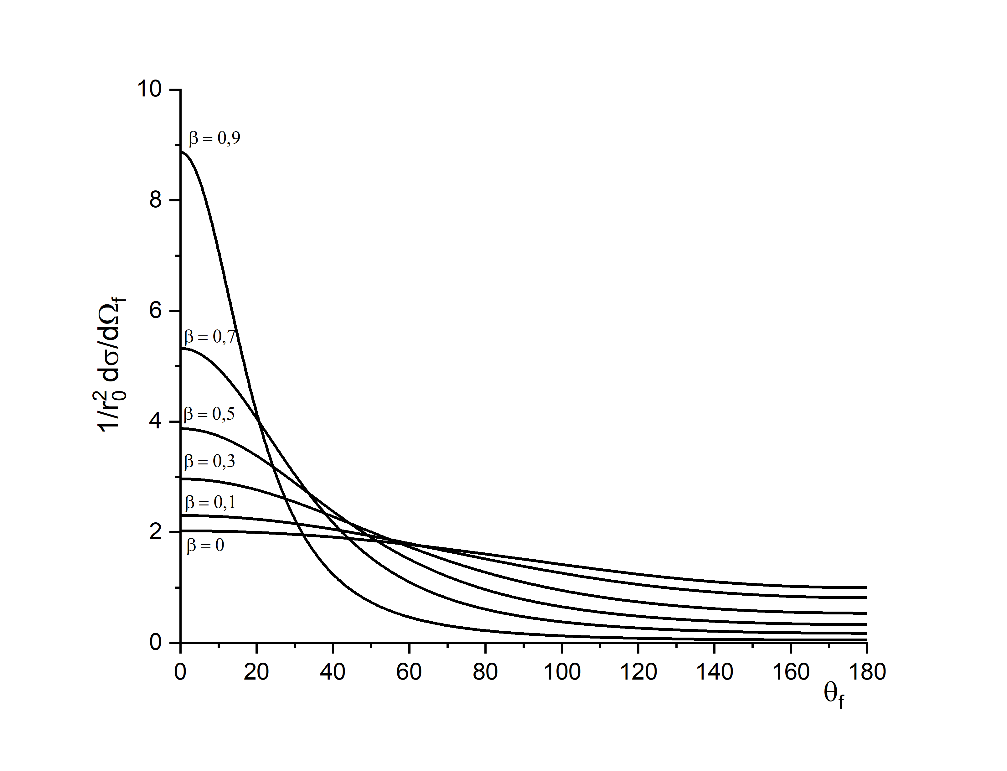
Figure 2: Left panel: Differential cross section (6.1) depending on the scattering angle $\theta_{f}$ for different values of $\beta$. The incident photon energy is $\omega_{i}=150$ keV, the angle is $\theta_{i}=180^{\circ}$ (head-on collision). Right panel: Averaged differential cross section (7), calculated taking into account Eqs. (6.1) and (3), $\theta_{i}=90^{\circ}$

This effect can be partly explained as follows. We expand cross section (7) into a series in Legendre polynomials $P_{l}(\cos\theta_{fi})$ and use the well-known formula

$$P_{l}(\cos\theta_{fi})=P_{l}(\cos\theta_{f})P_{l}(\cos\theta_{i})+2\sum_{m=1}^{l}\frac{(l-m)!}{(l+m)!}\ P_{l}^{m}(\cos\theta_{f})P_{l}^{m}(\cos\theta_{i})\cos m\Phi.$$

Integration with respect to the angle $\Phi$ removes the sum, and only the first term remains in the expansion. If the angle $\theta_{i}\sim 180^{\circ}$, then $P_{l}(-1)=\pm 1$ depending on the parity of $l$. If the angle $\theta_{i}\sim 90^{\circ}$, then the odd polynomials $P_{l}(0)=0$, while the even polynomials are not equal to 1. From a mathematical point of view, the difference in cross sections is explainable, but we still have no physical explanation.

A completely surprising situation with the cross section arises when $\theta_{i}=\theta_{f}=0$, i.e. the initial photons fly collinearly the electron beam and interact with it. The frequency of photons in this case does not change, but cross section (6.1) for forward scattering is equal to

$$\frac{d\sigma}{d\Omega_{f}}=r^{2}_{0}\frac{1+\beta}{1-\beta},$$

and grows infinitely in the ultrarelativistic case. This behavior is due to tending to zero with increasing energy of the denominator of the electron propagator between two vertices of the Feynman diagram, when the momenta of the photon and electron are parallel.

For a more detailed study of this interesting phenomenon, we plotted the dependence of differential cross section (6) on the angle of incidence of the photon $\theta_{i}$ on a moving electron for a fixed scattering angle $\theta_{f}=0$, which is presented in Fig. 3. The dependence on the angle $\Phi$ is absent in this case. In addition, in Fig. 3 we have presented, for convenience, graphs of frequency ratio $\omega_{f}/\omega_{i}$. From Fig. 3 it follows, that the cross section is practically constant at low electron velocities $\beta$ and the change in frequency is small. As $\beta$ grows, there appears a maximum in the cross section, which shifts to smaller angles of incidence of the photon with increasing $\beta$. At the same time, the change in frequency close to the maximum is, of course, significantly smaller than at the angle $\theta_{i}=180^{\circ}$.

This phenomenon is an unexpected and curious one, and has no direct relation to the inverse Compton effect with its goal to maximize the frequency of the final photon. However, we have found it to be interesting and tried to explain by carrying out a preliminary investigation of the derivative of cross section (6.1) with respect to $\cos\theta_{i}$ depending on $\beta$. It turned out that the maximum is already formed at $\beta\approx 0.2$ for $\cos\theta_{i}\sim-1$, i.e. for the geometry of backscattering. As $\beta$ increases, the value of $\cos\theta_{i}^{max}$ corresponding to the maximum of the cross section grows quite sharply, crosses zero at $\beta\approx 0.4$ and tends to one at asymptotic (ultrarelativistic) electron energies, and in this case $\cos\theta_{i}^{max}(\beta)\approx\beta$. We have obtained this result for the photon energy $\omega_{i}=150$ keV. A more complete study of this curious phenomenon requires consideration of other cases.

Figure 3: Differential cross section (6.1) calculated with taking into account formulas (6.2) and (3) depending on the angle of incidence of the photon $\theta_{i}$ for different $\beta$. The scattering angle is fixed, $\theta_{f}=0^{\circ}$. The incident photon energy is $\omega_{i}=150$ keV. Black (solid) lines show cross sections. For convenience, the red (dashed) lines show the ratio $\omega_{f}/\omega_{i}$.

POLARISATION EFFECTS

Let us now consider the influence of the polarizations of colliding particles on the cross section. In describing polarization effects, we use again the formulas from monograph [18]. We consider first the most common case of scattering of polarized photons at unpolarized electrons, where the polarizations of the final particles are not measured. The scattering plane of photons is given by the $(z,y)$ axes, and the $x$ axis is orthogonal to this plane. The degree of linear polarization is characterized by the Stokes parameter (the index $i$ refers to the initial photon or electron) $\xi_{3}^{(i)}=\cos 2\alpha$, where the angle $\alpha$ determines the polarization of the photon with respect to the $x$ axis. The photons polarized transverse to the scattering plane are characterized by the angle $\alpha=0$, in the scattering plane $\alpha=\pi/2$. The angle $\alpha=\pi/4$ corresponds to the absence of linear polarization.

In this case the cross section is also given by Eq. (6.1), where, however,

$$U_{0}(\xi_{3}^{(i)})=\left[4\left(\frac{1}{\kappa_{1}}+\frac{1}{\kappa_{2}}\right)^{2}-4\left(\frac{1}{\kappa_{1}}+\frac{1}{\kappa_{2}}\right)\right](1-\xi_{3}^{(i)})-\left(\frac{\kappa_{1}}{\kappa_{2}}+\frac{\kappa_{2}}{\kappa_{1}}\right),$$

Figure 4: Differential cross section (6.1) taking into account (8) depending on the scattering angle $\theta_{f}$ for different values of $\xi_{3}^{(i)}$. $I:\xi_{3}^{(i)}=1$; $II:\xi_{3}^{(i)}=0.5$; $III:\xi_{3}^{(i)}=0$; $IV:\xi_{3}^{(i)}=-0.5$; $V:\xi_{3}^{(i)}=-1$ . $\beta=0.7$. The incident photon energy is $\omega_{i}=150$ keV.

Examples of such cross sections are shown in Fig. 4. From the figure it follows that the largest cross section is achieved, when the photon is linearly polarized in the scattering plane, and, in this case, the cross section is much larger than for the other polarizations.

Next, we consider the scattering of a partially polarized photon by a partially polarized electron. The covariant form of the cross section in the approximation of interest to us looks as follows (since we do not consider the polarizations of the scattered particles, the cross section is multiplied by the factor of four):

$$\frac{d\sigma}{d\Omega_{f}}=2r^{2}_{0}\left(\frac{\omega_{f}}{mc^{2}\kappa_{1}}\right)^{2}[U_{0}(\xi_{3}^{(i)})+(f_{2})_{\mu}\xi^{(i)}_{2}s_{\mu}^{(i)}]$$

The first term is presented explicitly in formula (8) and has been considered above, the second term describes the scattering of partially circularly polarized photons by polarized electrons. The 4-vector $f_{2}$ entering it looks like:

$$(f_{2})_{\mu}=\frac{2}{mc}\left(\frac{1}{\kappa_{1}}+\frac{1}{\kappa_{2}}\right)\left[k_{i\mu}+k_{f\mu}-2\left(\frac{1}{\kappa_{1}}+\frac{1}{\kappa_{2}}\right)\ k_{i\mu}\right],$$

where $k_{\mu}=(\omega/c,\vec{k})$. It is necessary to remark that formula (10) is similar to formula (26.7.5) in monograph [18], which is misspelled and differs from formula (10) in the common sign that is due to the use of archaic notations in this monograph for the coordinates in Minkowski space with imaginary time component. In later editions of the monograph, a consideration of polarization effects involving a moving electron is absent at all, as well as in the most publications that we have looked through.

The Stokes parameter $\xi^{(i)}_{2}$ describes a partially circular polarization, and the components of the spin 4-vector of a moving electrons have the form

$$s_{0}=\frac{1}{mc}(\vec{p}\cdot\vec{\zeta}),\quad\vec{s}=\vec{\zeta}+\vec{p}\frac{(\vec{p}\cdot\vec{\zeta})}{mc(\sqrt{p^{2}+(mc)^{2}}+mc)}.$$

This formula gives the spin 4-vector $s$ in terms of the 3-dimensional polarization vector $\vec{\zeta}$ in the rest frame, which is convenient to be used for the parametrization of the spin vector.

Figure 5: Differential cross section (9) depending on the scattering angle $\theta_{f}$ for different values of the helicities of colliding particles for $\xi_{3}^{(i)}=0$ and several values of $\beta$. The incident photon energy is $\omega_{i}=150$ keV, its angle of incidence is $\theta_{i}=180^{\circ}$. Left panel: $\quad\xi_{2}^{(i)}\cdot\zeta^{(i)}_{\parallel}=1$; right panel: $\quad\xi_{2}^{(i)}\cdot\zeta^{(i)}_{\parallel}=-1$.

The general formula for the third term in (9) turns out to be quite cumbersome, so we will separately consider the longitudinal and transverse polarizations of the electron. For the transverse polarization

$$s_{0}^{(i)}=0,\quad\vec{s}^{(i)}=\vec{\zeta}^{(i)}_{\perp},\quad(\vec{p}_{i}\cdot\vec{\zeta}^{(i)}_{\perp})=0,\quad|\vec{\zeta}^{(i)}_{\perp}|\leq 1,$$

and for the longitudinal one

$$s_{0}^{(i)}=\frac{|\vec{p}_{i}|}{mc}\,\zeta^{(i)}_{\parallel},\quad\vec{s}^{(i)}=\frac{\vec{p}_{i}E_{i}}{|\vec{p}_{i}|mc^{2}}\,\zeta^{(i)}_{\parallel},\quad|\zeta^{(i)}_{\parallel}|\leq 1.$$

Besides that,

$$(\vec{k}_{i}\cdot\vec{p}_{i})=k_{i}p_{i}\cos\theta_{i},\quad(\vec{k}_{f}\cdot\vec{p}_{i})=k_{f}p_{i}\cos\theta_{f},$$

$$(\vec{k}_{i}\cdot\vec{\zeta}^{(i)}_{\perp})=\frac{1}{c}\ \omega_{i}\ \zeta^{(i)}_{\perp}\sin\theta_{i},\quad(\vec{k}_{f}\cdot\vec{\zeta}^{(i)}_{\perp})=\frac{1}{c}\ \omega_{f}\ \zeta^{(i)}_{\perp}\sin\theta_{f},$$

The last two formulas are written for the case, where the electron spin vector lies in the scattering plane, and $\zeta^{(i)}_{\perp}$ can take both positive and negative values.

As a result, for the transverse polarization of the electron in the scattering plane, after some transformations, the general formula can be rewritten as follows:

$$((f_{2})_{\mu}\xi^{(i)}_{2}s_{\mu}^{(i)})_{\perp}=-\xi^{(i)}_{2}\zeta^{(i)}_{\perp}\left(\frac{2\omega_{i}}{mc^{2}}\right)\left(\frac{1}{\kappa_{1}}+\frac{1}{\kappa_{2}}\right)\ \times$$

$$\left[\sin\theta_{i}\left(1-2\left(\frac{1}{\kappa_{1}}+\frac{1}{\kappa_{2}}\right)\right)+\frac{\omega_{f}}{\omega_{i}}\sin\theta_{f}\right],$$

and for the longitudinal polarization

$$((f_{2})_{\mu}\xi^{(i)}_{2}s_{\mu}^{(i)})_{\parallel}=\xi^{(i)}_{2}\zeta^{(i)}_{\parallel}\left(\frac{2\omega_{i}}{mc^{2}\sqrt{1-\beta^{2}}}\right)\left(\frac{1}{\kappa_{1}}+\frac{1}{\kappa_{2}}\right)\ \times$$

$$\left[(\beta-\cos\theta_{i})\left(1-2\left(\frac{1}{\kappa_{1}}+\frac{1}{\kappa_{2}}\right)\right)+\frac{\omega_{f}}{\omega_{i}}(\beta-\cos\theta_{f})\right].$$

From Eq. (12.1), in particular, it follows that if $\theta_{i}=\pi$ and $\theta_{f}=0$, then the transverse polarization of the electron does not contribute to the cross section at all.

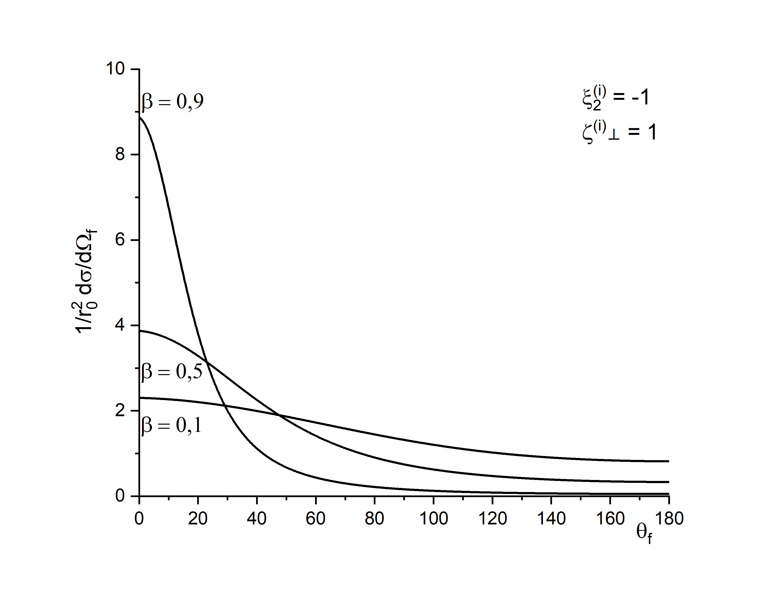
Figure 6: Differential cross section (9) depending on the scattering angle $\theta_{f}$ for different values of the polarizations of colliding particles: $\xi_{3}^{(i)}=0,\quad\xi_{2}^{(i)}=-1,\quad\zeta^{(i)}_{\perp}=1$, and for several values of $\beta$. The incident photon energy is $\omega_{i}=150$ keV, its angle of incidence is $\theta_{i}=180^{\circ}$.

Figs. 5,6 present examples of calculating differential cross section (9), where the linear polarization of the photon $\xi^{(i)}_{3}=0$. In Fig. 5 one sees the cross sections for the same and opposite helicities of photons and electrons. Because the polarization parameters enter cross section (12.2) as a product, then the cases $\xi^{(i)}_{2}\cdot\zeta^{(i)}_{\parallel}=\pm 1$ correspond to the same (opposite) helicities. Comparing Fig. 5 and 2 (left panel), we see that the electron helicity has a noticeable effect on the value of the cross section, and the maximum contribution to the cross section for the forward photon scattering is given by the polarization term with opposite photon and electron helicities. On the contrary, the same helicities of the particles noticeably reduce the cross sections.

As for the transverse polarization of the electron (Fig. 6), the contribution of the term $((f_{2})_{\mu}\xi^{(i)}_{2}s_{\mu}^{(i)})_{\perp}$ to cross section (9) is very small, and it changes very little the cross section compared to the unpolarized colliding particles shown in the left panel of Fig. 2. As a consequence, the sign of the photon helicity $\xi^{(i)}_{2}$ does not matter.

CONCLUSION

We have considered some kinematic conditions, including the polarizations of the colliding electron and photon, at which the maximum values of the differential cross section are reached at given electron and photon energies. It has been found that the cross section increases noticeably in the case of the electron spin being directed along its velocity and the left photon helicity, or vice versa.

Moreover, an unexpected effect of an increase in the cross section has been found for angles of incidence of photons on an electron beam different from $\pi$, while the final photons move along the beam. It has been shown that, as the angle of incidence of the photons decreases, the cross section increases and reaches a peak, the value of which increases with the growth of the electron energy, although such kinematics is not directly related to the classical inverse Compton effect.

ACKNOWLEDGEMENTS

The work was carried out with financial support of the Ministry of Science and higher education of the Russian Federation, project No.075-15-2021-1353.

References

- [1]
- [2] Compton A.H. // Phys. Rev. 1923. 21. P.483. https://doi.org/10.1103/PhysRev.21.483
- [3] DuMond J.W.M.// Phys. Rev. 1929. 33. P.643. https://doi.org/10.1103/PhysRev.33.643
- [4] Kircher M. et al. // Nature Phys. 2020.16. P.756. https://doi.org/10.1038/s41567-020-0880-2
- [5] Houamer S., Chuluunbaatar O., Volobuev I.P., Popov Yu.V. // Eur.Phys.Journ.D. 2020. 74. P.81. https://doi.org/10.1140/epjd/e2020-100572-1
- [6] Stepantsov I.S., Volobuev I.P., Popov Yu.V. // Moscow University Physics Bulletin (in russian). 2023 78(1), P. 2310404. https://doi.org/10.55959/MSU0579-9392.78.2310404
- [7] Burtelov V.A., Kudryashov A.V., Sheshin E.P., Majmaa H.K.K. // Moscow Institute of Physics and Technology Proceedings (in russian). 2019 11(2), P. 116.
- [8] Artyukov I.A., Vinogradov A.V., Feshchenko R.M. // Physical Basis of Instrumentation (in russian). 2016 5(3), P. 56. https://doi.org/10.25210/jfop-1603-056069
- [9] Miscellany // Compton effect on the nucleon at low and medium energies. The P.N. Lebedev Physical Institute Proceedings (in russian). 1968 41, Moscow: Nauka.
- [10] Baranov P.S., Fil’kov L.V., Sokol G.A. // Fortschritte der Physik 1968, 16(11-12), P.595. https://doi.org/10.1002/prop.19680161102
- [11] Ginzburg V.L., Syrovatskii S.I.// JETP 1964 19(5), P. 1255.
- [12] Jones F.C. // Phys. Rev. 1968 167, P. 1159. https://doi.org/10.1103/PhysRev.167.1159
- [13] Blumenthal G.R., Gould R.J.// Rev. Mod. Phys. 1970 42(2), P. 237. https://doi.org/10.1103/RevModPhys.42.237
- [14] Berezinskii V.S., Bulanov S.V., Dogiel V.A., Ptuskin V.S.// Astrophysics of cosmic rays. Amsterdam: North-Holland (edited by Ginzburg V.L.) 1990, 360 pp.
- [15] Fargion D, Salis A // Phys. Usp. 1998 41, P. 823. https://doi.org/10.1070/PU1998v041n08ABEH000432
- [16] Hütt M.-Th., L’vov A.I., Milstein A.I., Schumacher M. // Physics Reports 2000, 323(6), P.457. https://doi.org/10.1016/S0370-1573(99)00041-1
- [17] STAR Collaboration, // Sci. Adv. 2023 9(1), P. 3903. https://doi.org/10.1126/sciadv.abq3903
- [18] Akhiezer A.I., Berestetskii V.B. // Quantum Electrodynamics (in russian). Moscow: Nauka, 1969, 623 pp., §§ 26-27.
- [19] Kurnosova L.V. (in russian) // UFN 1954 LII (4), P. 603. https://doi.org/10.3367/UFNr.0052.195404c.0603
- [20] Nedorezov V.G., Turinge A.A., Shatunov Yu.M.// Physics Uspekhi 2004 47(4), P. 341. https://doi.org/10.1070/PU2004v047n04ABEH001743