Relativistic stochastic mechanics I:
Langevin equation from observer’s perspective

Abstract

Two different versions of relativistic Langevin equation in curved spacetime background are constructed, both are manifestly general covariant. It is argued that, from the observer’s point of view, the version which takes the proper time of the Brownian particle as evolution parameter contains some conceptual issues, while the one which makes use of the proper time of the observer is more physically sound. The two versions of the relativistic Langevin equation are connected by a reparametrization scheme. In spite of the issues contained in the first version of the relativistic Langevin equation, it still permits to extract the physical probability distributions of the Brownian particles, as is shown by Monte Carlo simulation in the example case of Brownian motion in $(1+1)$-dimensional Minkowski spacetime.

1 Introduction

General relativity and non-equilibrium statistical physics are two important frontiers of modern theoretical physics. In spite of the significant progresses in their respective fields, the study on the overlap between these two fields remains inactive. However, owing to the development in astrophysics, there are more and more scenarios in which both general relativity and non-equilibrium statistical physics are important. Therefore, it becomes necessary and of utmost importance to take the combination of general relativity and non-equilibrium statistical physics more seriously.

There are two major branches in non-relativistic non-equilibrium statistical physics, i.e. kinetic theory and stochastic mechanics. The study of kinetic theory started from Boltzmann’s works, and its relativistic version also has a long history (which can be traced back to Jüttner’s works in 1911 [1]). Currently, the framework of relativistic kinetic theory looks fairly complete [2, 3, 4, 5]. In contrast, the study of relativistic stochastic mechanics is still far from being accomplished. Since the relativistic Ornstein-Uhlenbeck process was proposed about 20 years ago[6], there appeared some attempts in relativistic stochastic mechanics [7, 8, 9, 10, 11, 12, 13, 14, 15], mostly in the special relativistic regime. However, apart from Herrmann [14, 15] and Haba’s [16] works, the manifest covariance of stochastic mechanics is typically absent. Some work [11] considered concrete curved spacetime background without paying particular attention to general covariance. There are also some other works which focus on the covariance of stochastic thermodynamics [17, 18], but those works have nothing to do with relativity.

The random motion of heavy particles began to attract scientific interests in the late 19th and early 20th centuries, as it provides a simple example for the diffusion phenomena. Einstein [19, 20] and Smoluchowski [21] showed that the random motion is closely related to macroscopic environment, however, the microscopic description of the random motion has not been established. Later, Langevin [22] wrote down the first equation of motion for a Brownian particle by his physical intuition, which inspired subsequent explorations about the microscopic mechanisms of Brownian motion. In the 1960-1970s, a series of models [23, 24, 25] were proposed in this direction, which made it clear why the disturbance from the heat reservoir could be viewed as Gaussian noises, and hence a bridge between microscopic mechanical laws and non-equilibrium macroscopic phenomena is preliminarily established in the non-relativistic regime. Since the 1990s, the so-called stochastic thermodynamics based on top of Langevin equation was established [26, 27].

To some extent, the challenge in constructing a covariant Langevin equation arises from the underestimation about the role of the observer. Unlike general relativity which concentrates mainly on the universal observer independent laws about the spacetime, statistical physics concentrates more on the observational or phenomenological aspects, which are doomed to be observer dependent. The lack of manifest covariance in some of the works on relativistic Langevin equation, e.g. [6, 7, 8, 9, 10], stems from the choice of the coordinate time as evolution parameter. As exceptional examples, Herrmann [14, 15] and Haba’s [16] work adopted the proper time of the Brownian particle evolution parameter and the corresponding versions of Langevin equation are indeed manifestly covariant. Nevertheless, the role of the observer is still not sufficiently stressed in those works, and it will be clear that, from the observer’s point of view, the proper time of the Brownian particle should not be thought of as an appropriate evolution parameter. The present work aims to improve the situation by reformulating the relativistic Langevin equation from the observer’s perspective and taking the observer’s proper time as evolution parameter. In this way, we obtain the general relativistic Langevin equation which is both manifestly general covariant and explicitly observer dependent.

This work is Part I of a series of two papers under the same main title “Relativistic stochastic mechanics”. Part II will be concentrated on the construction of Fokker-Planck equations associated with the Langevin equations presented here.

This paper is organized as follows. In Sec.2, we first clarify certain conceptual aspects of relativistic mechanics which are otherwise absent in the non-relativistic context. These include the explanation on the role of observers, the choice of time and the conventions on the space of micro states (SoMS). Sec.3 is devoted to a first attempt for the construction of general relativistic Langevin equation. To make the discussions self contained, we start from a brief review about the non-relativistic Langevin equation, and then pay special attentions toward the form of the damping and additional stochastic forces in the relativistic regime. As the outcome of these analysis, we write down a first candidate for the relativistic Langevin equation [referred to as LE_τ], which is manifestly general covariant. It is checked that the stochastic motion of the Brownian particle following this version of the Langevin equation does not break the mass shell condition. However, since this version of the relativistic Langevin equation employs the proper time $\tau$ of the Brownian particle as evolution parameter, there are still some issues involved in it, because, from the observer’s point of view, $\tau$ itself is a random variable, which is inappropriate to be taken as an evolution parameter. The problem with LE_τ is resolved in Sec.4 by introducing a reparametrization scheme, which yields another version of the relativistic Langevin equation [LE_t], which employs the proper time $t$ of the prescribed observer as evolution parameter. In Sec.5, the stochastic motion of Brownian particles in $(1+1)$-dimensional Minkowski spacetime driven by a single Wiener process and subjects to an isotropic homogeneous damping force is analyzed by means of Monte Carlo simulation. It is shown that, in spite of the issues mentioned above, LE_τ still permits for exploring the physical probability distributions, and the resulting distributions are basically identical to those obtained from LE_t. Finally, we present some brief concluding remarks in Sec.6.

2 Observers, time, and the SoMS

As mentioned earlier, we are interested in describing the stochastic motion of Brownian particles in a generic spacetime manifold $\mathcal{M}$. To achieve this goal, a fully general covariant description for the SoMS and equations of motion are essential.

Determining a micro state of a classical physical system requires the simultaneous determination of the concrete position and momentum of each individual particle at a given instance of time. In Newtonian mechanics, there is an absolute time, therefore, there is no ambiguity as to what constitutes a “given instance of time”. However, in relativistic regime, the concept of simultaneity becomes relative, and in order to assign a proper meaning for a micro state, one needs to introduce a concrete time slicing (or temporal foliation) of the spacetime at first. There are two approaches to do so, i.e. (1) choosing some coordinate system and making use of the coordinate time as the slicing parameter; (2) introducing some properly aligned observer field and choosing the proper velocity $Z^{\mu}$ ($Z^{\mu}Z_{\mu}=-1$) of the observer field as normalized normal vector field of the spatial hypersurfaces consisting of “simultaneous events”, which is also referred to as the configuration space. Let us recall that an observer in a generic $(d+1)$-dimensional spacetime manifold $\mathcal{M}$ is represented by a timelike curve with normalized future-directed tangent vector $Z^{\mu}$ which is identified as the proper velocity of the observer. An observer field is a densely populated collection of observers whose worldlines span the full spacetime. The second slicing approach is always possible because each observer naturally carries a Frenet frame with orthonormal basis $e^{\mu}{}_{\hat{\nu}}$ with $e^{\mu}{}_{\hat{0}}:=Z^{\mu}$, and, as one of the basis vector field, $Z^{\mu}$ naturally satisfies the Frobenius theorem

$$Z_{[\mu}\nabla_{\nu}Z_{\rho]}=0,$$

which in turn implies the existence of spacelike hypersurfaces which take $Z^{\mu}$ as normal vector field.

In practice, the two time slicing approaches can be made identical. One only needs to choose the specific observers whose proper velocity covector field $Z_{\mu}$ is proportional to $({\rm d}{x^{0}})_{\mu}$. However, such an identification often obscures the role of the observer field and brings about the illusion that the corresponding description is necessarily coordinate dependent and lacks the spacetime covariance. Therefore, it will be preferable to take the choice of not binding the coordinate system and the observer field together and focusing on explicit general covariance.

While an observer field can be used to identify which events happens simultaneously, it cannot uniquely specify the timing of the configuration spaces. To achieve this, we need to pick a single observer, referred to as Alice, from the set of observers. The integral curve of this particular observer can be denoted as $x^{\mu}(t)$, where $t$ represents the proper time of this single observer. In principle, we can extend $t$ into a smooth scalar field $t(x)$ over the whole spacetime manifold, such that we can label the configuration space at the proper time $t$ of Alice unambiguously as the hypersurface $\mathcal{S}_{t}:=\{x\in{\mathcal{M}}|t(x)=t={\rm const}.\}$. The union of $\mathcal{S}_{t}$ at all possible $t$ covers $\mathcal{M}$. Notice that, in general, $t$, $x^{0}$ (the zeroth component of the coordinate system) and $\tau$ (the proper time of the Brownian particle) can all be different entities.

The momentum of a relativistic particle is a tangent vector of the spacetime manifold $\mathcal{M}$. Accordingly, the momentum space of a particle should be a subset of the tangent bundle $T\mathcal{M}$ of the spacetime, because the momentum must obey the mass shell condition

$$S(x,p):=p^{\mu}p_{\mu}+m^{2}=g_{\mu\nu}(x)p^{\mu}p^{\nu}+m^{2}=0.$$ (1)

Moreover, the momentum of a massive particle must be a future-directed timelike vector, i.e. $p^{\mu}Z_{\mu}(x)<0$. Putting these requirements together, we conclude that the SoMS of a massive relativistic particle must be a subspace of the future mass shell bundle $\Gamma^{+}_{m}$,

$$\Gamma^{+}_{m}:=\{(x,p)\in T\mathcal{M}|\ g_{\mu\nu}(x)p^{\mu}p^{\nu}=-m^{2}\ \text{and}\ p^{\mu}Z_{\mu}(x)<0\}.$$

The geometry of future mass shell bundle is decided by the Sasaki metric[28], and its associated volume element is

$$\eta_{\Gamma^{+}_{m}} =\frac{\det(g)}{p_{0}}{\rm d}x^{0}\wedge{\rm d}x^{1}\wedge...\wedge{\rm d}x^{d}\wedge{\rm d}p^{1}\wedge...\wedge{\rm d}p^{d}.$$ (2)

The momentum space at the event $x\in\mathcal{M}$ is simply the fiber of the future mass shell bundle $\Gamma^{+}_{m}$ at the base point $x$,

$$(\Gamma^{+}_{m})_{x}:=T_{x}\mathcal{M}\cap\Gamma^{+}_{m}.$$

Please be aware that the SoMS of a massive relativistic particle is not the full future mass shell bundle $\Gamma^{+}_{m}$, because the configuration space is only the spacelike hypersurface $\mathcal{S}_{t}$ consisted of simultaneous events regarding to the proper time $t$ of Alice. Therefore, the actual SoMS should be the proper subspace

$$\Sigma_{t}:=\bigcup_{x\in\mathcal{S}_{t}}(\Gamma_{m}^{+})_{x}=\{(x,p)\in\Gamma^{+}_{m}|x\in\mathcal{S}_{t}\}$$

of the full future mass shell bundle $\Gamma^{+}_{m}$.

Due to the mass shell condition, the actual momentum space $(\Gamma^{+}_{m})_{x}$ has one less dimension than the tangent space $T_{x}\mathcal{M}$. It will be appropriate to think of $(\Gamma^{+}_{m})_{x}$ as a codimension one hypersurface in $T_{x}\mathcal{M}$ defined via eq.(1), and its (unmormalized) normal covector can be defined as $\mathcal{N}_{\mu}:=\frac{\partial}{\partial p^{\mu}}S(x,p)=2p_{\mu}$. In view of this, any tangent vector field $\mathcal{V}\in T[(\Gamma^{+}_{m})_{x}]$ must be normal to $p_{\mu}$, i.e., $\mathcal{V}^{\mu}p_{\mu}=0$. Using this property, we can select a basis for the tangent space of the momentum space, i.e.

$$\dfrac{\partial}{\partial\breve{p}^{i}}:=\dfrac{\partial}{\partial{p}^{i}}-\dfrac{p_{i}}{p_{0}}\dfrac{\partial}{\partial{p}^{0}}.$$

Therefore, the tangent vector field $\mathcal{V}\in T[(\Gamma^{+}_{m})_{x}]$ acquires two component-representations, one in the basis $\dfrac{\partial}{\partial p^{\mu}}$ of $T(T_{x}\mathcal{M})$, and one in the basis $\dfrac{\partial}{\partial\breve{p}^{i}}$ of $T[(\Gamma^{+}_{m})_{x}]$. It is easy to check that these two representations are equivalent,

$$\mathcal{V}^{i}\frac{\partial}{\partial\breve{p}^{i}}=\mathcal{V}^{i}\frac{\partial}{\partial p^{i}}-\mathcal{V}^{i}\frac{p_{i}}{p_{0}}\frac{\partial}{\partial p^{0}}=\mathcal{V}^{i}\frac{\partial}{\partial p^{i}}+\mathcal{V}^{0}\frac{\partial}{\partial p^{0}}=\mathcal{V}^{\mu}\dfrac{\partial}{\partial p^{\mu}}.$$ (3)

Therefore, when describing a vector in $T[(\Gamma^{+}_{m})_{x}]$, the two component-representations $\mathcal{V}^{i}$ and $\mathcal{V}^{\mu}$ can be used interchangeably.

3 The covariant Langevin equation

3.1 A short review of Langevin equation in non-relativistic setting

The main focus of this section is to construct a covariant Langevin equation in a generic spacetime. Before dwelling into the detailed construction, it seems helpful to make a brief review of Langevin equation in the non-relativistic setting.

The non-relativistic Langevin equation describes the motion of a Brownian particle in a fixed heat reservoir. The initial intuitive construction of Langevin equation is simply based on the second law of Newtonian mechanics, in which the motion of the Brownian particle is driven by drift and damping forces $F_{\rm drift}(x)$, $F_{\rm damp}(p)$ together with a random force $\xi(t)$. The drift force $F_{\rm drift}(x)$ is provided by a conservative potential and hence is dependent on the coordinate position $x$ of the Brownian particle. The damping force $F_{\rm damp}(p)$, however, is dependent on the momentum of the particle. In the absence of the drift force, the Langevin equation describing one-dimensional Brownian motion can be intuitively written as

$$\dfrac{{\rm d}p}{{\rm d}t}=F_{\rm damp}(p)+\xi(t).$$ (4)

However, it was soon realized that this intuitive picture cannot be mathematically correct, because, under the impact of the random force, the momentum of the Brownian particle cannot be differentiable with respect to the time $t$, and hence the Langevin equation cannot actually be regarded as a differential equation.

The modern understanding of Langevin equation is as follows. Consider a scenario in which a large number of light particles exist in the heat reservoir, and they randomly collide with the heavy Brownian particle, causing the momentum of the latter to alter with each collision. If the mass ratio between the Brownian particle and the particle from the heat reservoir is sufficiently large, there will be a timescale ${\rm d}t$ during which a sufficiently large number of independent collisions happen. Since the Brownian particle is heavy, its state changes very little within this timescale. According to the central limit theorem, the probability distribution of the variations of the momentum during ${\rm d}t$ follows a Gaussian distribution. The average value of this distribution yields the damping force $F_{\rm damp}$, while the remaining (rapid) portion is viewed as a stochastic force. Thus, the classical Langevin equation in one-dimensional space can be expressed as

$${\rm d}\tilde{x}_{n} =\frac{\tilde{p}_{n}}{m}{\rm d}t$$

$${\rm d}\tilde{p}_{n} =R{\rm d}\tilde{w}_{n}+F_{\rm damp}{\rm d}t,$$ (5)

where the suffices $n$ represents the $n$-th time step and ${\rm d}\tilde{w}_{n}$ is a random variable obeying Gaussian distribution

$$\Pr[{\rm d}\tilde{w}_{n}={\rm d}w_{n}]=\frac{1}{\sqrt{2\pi{\rm d}t}}{\rm e}^{-\frac{1}{2}\frac{{\rm d}w_{n}^{2}}{{\rm d}t}}.$$

The coefficient $R$ appeared in eq.(5) is called stochastic amplitude. Notice that the variance of the above Gaussian distribution equals ${\rm d}t$. In this paper, tilded variables such as $\tilde{x},\tilde{p}$ represent random variables, and the corresponding un-tilded symbols (e.g. $x,p$) represent their concrete realizations.

The Langevin equation as presented above is technically a system of discrete-time difference equations, as the time scale ${\rm d}t$ must be large enough to permit sufficient number of collisions to happen during this time interval. However, if ${\rm d}t$ is far smaller than the relaxation time, it can be effectively thought of as infinitesimal. In the limit of continuity, $\tilde{w}_{n}$ becomes a Wiener process $\tilde{w}_{t}$, and there is an ambiguity in the coupling rule between the stochastic amplitude $R$ and the Wiener process if $R$ is dependent on the momentum. Unlike in normal calculus, in the continuity limit,

$$R(\tilde{p}_{n}+a{\rm d}\tilde{p}_{n}){\rm d}\tilde{w}_{n}\xlongrightarrow[]{{\rm d}t\rightarrow 0}R(\tilde{p}_{t})\circ_{a}{\rm d}\tilde{w}_{t}$$ (6)

depends on the value of $a\in[0,1]$ [29]. The continuum version of Langevin equation with the above coupling rule reads

$${\rm d}\tilde{x}_{t} =\frac{\tilde{p}_{t}}{m}{\rm d}t$$

$${\rm d}\tilde{p}_{t} =R(\tilde{p}_{t})\circ_{a}{\rm d}\tilde{w}_{t}+F_{\rm damp}{\rm d}t.$$ (7)

In particular, the coupling rule with $a=0$ is known as Ito’s rule and is denoted as $R\circ_{I}{\rm d}\tilde{w}_{t}$, while the rule with $a=1/2$ is known as Stratonovich’s rule and is denoted as $R\circ_{S}{\rm d}\tilde{w}_{t}$.

Ito’s rule allows Langevin equation to be understood as an equation describing a Markov process, making it easier to analyze. However, since ${\rm d}t$ is equal to the variance of the Wiener process, ${\rm d}\tilde{w}_{t}$ should be in the same order of magnitude with $\sqrt{{\rm d}t}$. This fact leads to some profound consequences. For instance, it can be easily verified that any coupling rule $\circ_{a}$ can be related to Ito’s rule via

$$R(\tilde{p}_{t})\circ_{a}{\rm d}\tilde{w}_{t}=R(\tilde{p}_{t})\circ_{I}{\rm d}\tilde{w}_{t}+aR\frac{\partial}{\partial p}R\,{\rm d}t,$$

which is a straightforward consequence of eq.(6). Moreover, it can also be checked that Ito’s rule breaks the chain rule of calculus,

$${\rm d}h(\tilde{p}_{t}) =\frac{\partial h}{\partial p}{\rm d}\tilde{p}_{t}+\frac{1}{2}\frac{\partial^{2}h}{\partial p^{2}}{\rm d}\tilde{p}_{t}^{2}$$

$$=\left(\frac{\partial h}{\partial p}F_{\rm damp}+\frac{1}{2}\frac{\partial^{2}h}{\partial p^{2}}R^{2}\right){\rm d}t+\frac{\partial h}{\partial p}R(\tilde{p}_{t})\circ_{I}{\rm d}\tilde{w}_{t}\neq\frac{\partial h}{\partial p}{\rm d}\tilde{p}_{t}.$$

On the other hand, Stratonovich’s rule is the unique rule that preserves the chain rule,

$${\rm d}h(\tilde{p}_{t}) =\frac{\partial h}{\partial p}{\rm d}\tilde{p}_{t}+\frac{1}{2}\frac{\partial^{2}h}{\partial p^{2}}{\rm d}\tilde{p}_{t}^{2}$$

$$=\frac{\partial h}{\partial p}\left(R(\tilde{p}_{t})\circ_{a}{\rm d}\tilde{w}_{t}+F_{\rm damp}{\rm d}t\right)+\frac{1}{2}\frac{\partial^{2}h}{\partial p^{2}}\left(R(\tilde{p}_{t})\circ_{a}{\rm d}\tilde{w}_{t}+F_{\rm damp}{\rm d}t\right)^{2}$$

$$=\left(\frac{\partial h}{\partial p}F_{\rm damp}+a\frac{\partial h}{\partial p}R\frac{\partial}{\partial p}R+\frac{1}{2}\frac{\partial^{2}h}{\partial p^{2}}R^{2}\right){\rm d}t+\frac{\partial h}{\partial p}R(\tilde{p}_{t})\circ_{I}{\rm d}\tilde{w}_{t}$$

$$\xlongequal[]{a={1}/{2}}\frac{\partial h}{\partial p}F_{\rm damp}{\rm d}t+\frac{1}{2}\frac{\partial h}{\partial p}R\frac{\partial}{\partial h}\left(\frac{\partial h}{\partial p}R\right){\rm d}t+\frac{\partial h}{\partial p}R(\tilde{p}_{t})\circ_{I}{\rm d}\tilde{w}_{t}$$

$$=\frac{\partial h}{\partial p}F_{\rm damp}{\rm d}t+\frac{\partial h}{\partial p}R\circ_{S}{\rm d}\tilde{w}_{t}=\frac{\partial h}{\partial p}{\rm d}\tilde{p}_{t},$$

where, in the last step, we used the Langevin equation which adopts Stratonovich’s rule. Since the tensor calculus on manifolds is strongly dependent on the chain rule, it is natural to adopt Stratonovich’s rule while constructing the general covariant Langevin equation on a generic spacetime manifold, as we will do in the subsequent analysis. Other elaborations on the covariance of Stratonovich type stochastic differential equations can be found in Refs. [30, 31, 32].

3.2 Nonlinear damping force and additional stochastic force

Let us now consider the Langevin equation (7) with Ito’s rule and make a comparison with the intuitive form (4) of the equation. In essence, both the damping force $F_{\rm damp}$ and “stochastic force” $\xi(t)=R\circ_{I}{\rm d}\tilde{w}/{\rm d}t$ arise from the collisions between the Brownian particle and the heat reservoir particles, however, we have artificially separated them. It is possible to derive the expressions of $R$ and $F_{\rm damp}$ directly from microscopic mechanics and the chaotic assumption of the heat reservoir [24, 25]. Macroscopically, the stochastic force can be viewed as the consequence of thermal fluctuations, and thus it vanishes in the low temperature limit. In such surroundings, the damping force can be measured directly, allowing us to construct simple phenomenological models. The simplest one assumes a linear damping force proportional to the momentum of the Brownian particle in the reference frame comoving with the heat reservoir:

$$F_{\rm damp}=-Kp,$$

where $K$ is the damping coefficient. This simple model captures two important features of the damping force: First, when the Brownian particle comoves with the heat reservoir, the damping force vanishes. Second, the direction of the damping force should be opposite to the relative velocity. In more general cases than the linear damping model, the damping coefficient $K$ could be dependent on the momentum $p$ of the Brownian particle.

If $K$ is independent of $p$, the stochastic amplitude $R$ can be easily derived using the thermal equilibrium between the Brownian particle and the heat reservoir, yielding

$$D:=R^{2}=2\,TK,$$

where $T$ is the temperature of the reservoir. This relation is known as the Einstein relation. However, for nonlinear damping forces, the situations become much more complicated. Ref.[33] demonstrated that, provided $R$ is momentum dependent, there exists a non-zero force $\frac{1}{2}{\partial(R^{2})}/{\partial p}$ acting on the Brownian particle even if its momentum vanishes. This extra force term is also a consequence of the thermal equilibrium between the Brownian particle and the heat reservoir. There are two options for interpreting this extra force. The first option is to consider it as a part of the damping force, so that the full damping force takes the form

$$F_{\rm damp}=R\frac{\partial}{\partial p}R-Kp=-K_{\text{eff}}\,p,$$

where the effective damping coefficient reads

$$K_{\text{eff}}:=K-\frac{R}{p}\frac{\partial}{\partial p}R.$$

Consequently, there will be a modified Einstein relation

$$R^{2}=2T\left[K_{\text{eff}}+\frac{R}{p}\frac{\partial}{\partial p}R\right].$$

This option seems to have several issues. (1) It looks strange that the damping force still exists when the momentum is zero; (2) More importantly, we cannot define an effective damping coefficient in higher spatial dimensions using this approach. The second option is to split the extra force term $\frac{1}{2}{\partial R^{2}}/{\partial p}$ into two equal halves: one half is to be combined with the Ito’s coupling to give rise to Stratonovich’s coupling with Gaussian noises, and the other half is understood as an “additional stochastic force”

$$F_{\text{add}}:=\frac{1}{2}R\frac{\partial}{\partial p}R.$$

Hence, the more general Langevin equation in $d$-dimensional flat space can be written as

$${\rm d}\tilde{x}^{i}_{t} =\frac{\tilde{p}^{i}_{t}}{m}{\rm d}t$$

$${\rm d}\tilde{p}^{i}_{t} =\left[R^{i}{}_{\mathfrak{a}}\circ_{S}{\rm d}\tilde{w}_{t}^{\mathfrak{a}}+F^{i}_{\text{add}}{\rm d}t\right]-K^{i}{}_{j}\tilde{p}^{j}_{t}{\rm d}t,$$

where the indices $i,j$ label different spatial dimensions and $\mathfrak{a},\mathfrak{b}$ are used to distinguish independent Gaussian noises. It should be remarked that the number $\mathfrak{d}$ of Gaussian noises is independent of the dimension $d$ of the space. The additional stochastic force now reads

$$F^{i}_{\text{add}}=\frac{\delta^{\mathfrak{a}\mathfrak{b}}}{2}R^{i}{}_{\mathfrak{a}}\frac{\partial}{\partial p^{j}}R^{j}{}_{\mathfrak{b}}.$$ (8)

The discussions made so far in this subsection have been restricted to the non-relativistic situations. In the next subsection, it will be clear that the mass shell condition in the relativistic setting requires that the damping coefficients have to be momentum dependent. Therefore, the additional stochastic force should also appear in the relativistic Langevin equation. To derive the concrete expression for this additional stochastic force, we need to make use of the Fokker-Planck equation and the relativistic Einstein relation. However, since the focus of the present work is on the relativistic Langevin equation, we will provide the detailed derivation in Part II of this series of works. At present, we simply provide the result,

$$\mathcal{F}^{\mu}_{\text{add}}=\frac{\delta^{\mathfrak{a}\mathfrak{b}}}{2}\mathcal{R}^{\mu}{}_{\mathfrak{a}}\nabla^{(h)}_{i}\mathcal{R}^{i}{}_{\mathfrak{b}},$$ (9)

where $h$ refers to the metric on the mass shell $(\Gamma^{+}_{m})_{x}$. It is important to note that the stochastic amplitudes $\mathcal{R}^{\mu}{}_{\mathfrak{a}}$ in the relativistic Langevin equation should be a set of vectors on the curved Riemannian manifold $(\Gamma^{+}_{m})_{x}$, i.e. $\mathcal{R}^{\mu}{}_{\mathfrak{a}}\in T[(\Gamma^{+}_{m})_{x}]$. As such, the derivative operator $\partial/\partial p^{i}$ that appeared in eq.(8) needs to be replaced by the covariant derivative $\nabla^{(h)}_{i}$ on the momentum space $(\Gamma^{+}_{m})_{x}$.

3.3 Relativistic damping force

Recall that the damping force arises from the interaction between the Brownian particle and the heat reservoir, but only accounts for a portion of the total interaction, neglecting thermal fluctuations. We can directly measure the damping force when the thermal fluctuations can be ignored and establish a phenomenological model. It is reasonable to expect that the damping force should vanish if the Brownian particle comoves with the heat reservoir. Hence, the damping force can be regarded as an excitation of the relative velocity, with the damping coefficients serving as response factors. This idea was also explored in previous works [6, 8] in the special relativistic context. Here we shall extend the construction to the general relativistic case and point out some crucial subtleties which need to be taken care of.

In the relativistic context (be it special or general), the concept of velocity is replaced by proper velocity. However, the relative velocity cannot be defined simply as the difference between two proper velocities, because the temporal component of the difference should not be considered as part of the relative velocity but rather as the energy difference. In order to have an appropriate definition for the relative velocity, one must project one of the two proper velocities onto the orthonormal direction of the other. Let $U^{\mu}$ be the velocity of the heat reservoir and $p^{\mu}$ be the proper momentum of the Brownian particle. One can associate with the Brownian particle an orthonormal projection tensor

$$\Delta^{\mu}{}_{\nu}(p):=\delta^{\mu}{}_{\nu}+\frac{p^{\mu}p_{\nu}}{m^{2}}$$

which obeys

$$\Delta^{\mu}{}_{\nu}(p)p^{\nu}=0.$$

Then the relative velocity between the Brownian particle and the heat reservoir can be defined as $\Delta^{\mu}{}_{\nu}(p)U^{\nu}$. This definition has two important features, i.e. (1) when the Brownian particle is comoving with the heat reservoir, the relative velocity vanishes; (2) the relative velocity is always normal to $p_{\mu}$, so that it is a vector in $T[(\Gamma^{+}_{m})_{x}]$.

The relativistic damping force needs to have the following properties. First, it must contain the relative velocity as a factor, and a tensorial damping coefficient $\mathcal{K}^{\mu\nu}$ as another factor, i.e.

$$\mathcal{F}^{\mu}_{\rm damp}=\mathcal{K}^{\mu\nu}\Delta_{\nu}{}^{\rho}(p)U_{\rho}.$$

Second, the damping force needs to be a tangent vector of the momentum space $(\Gamma^{+}_{m})_{x}$, i.e. $\mathcal{F}^{\mu}\in T[(\Gamma^{+}_{m})_{x}]$. This latter requirement implies that $\mathcal{K}^{\mu\nu}$ must satisfy the relation

$$\mathcal{K}^{\mu\nu}(x,p)=\Delta^{\mu}{}_{\alpha}(p)\mathcal{K}^{\alpha\beta}(x,p)\Delta_{\beta}{}^{\nu}(p).$$ (10)

In the light of eq.(10) and the idempotent property of the projection tensor, the relativistic damping force can be simply rewritten as

$$\mathcal{F}^{\mu}_{\rm damp}=\mathcal{K}^{\mu\nu}U_{\nu}.$$ (11)

The constraint condition (10) over the tensorial damping coefficient has a very simple special solution

$$\mathcal{K}^{\mu\nu}=\kappa(x,p)\Delta^{\mu\nu}(p),$$

where $\kappa(x,p)$ is a scalar function on the SoMS $\Sigma_{t}$ and is referred to as the friction coefficient. This particular choice of damping coefficient corresponds to isotropic damping force. If $\kappa(x,p)$ is constant, then damping force will become homogeneous. Therefore, the isotropic homogeneous damping force can be written as

$$\mathcal{F}^{\mu}_{\rm damp}=\kappa\Delta^{\mu}{}_{\nu}(p)U^{\nu}.$$

Let $e^{\mu}{}_{\hat{i}}$ be the spatial comoving frame covectors associated with the Brownian particle and $E^{\hat{i}}{}_{\nu}$ be the dual vectors. Then the projection tensor $\Delta^{\mu}{}_{\nu}(p)$ can be written as

$$\Delta^{\mu}{}_{\nu}(p)=e^{\mu}{}_{\hat{i}}E^{\hat{i}}{}_{\nu}.$$

The isotropic homogeneous damping force can be re-expressed as

$$\mathcal{F}^{\mu}_{\rm damp}=\kappa e^{\mu}{}_{\hat{i}}E^{\hat{i}}{}_{\nu}U^{\nu}={\kappa U^{\hat{i}}}e^{\mu}{}_{\hat{i}},$$

or more concisely as

$$\mathcal{F}^{\hat{i}}_{\rm damp}=\kappa U^{\hat{i}},$$

where $\mathcal{F}^{\hat{i}}_{\rm damp}=\mathcal{F}^{\mu}_{\rm damp}E^{\hat{i}}{}_{\mu}$, which represents the spatial components of the damping force under the comoving frame. This equation has the same form as the one given in [8, 9]. However, our expression (11) for the damping force is more general and does not rely on a particular choice of frame basis.

3.4 Covariant relativistic Langevin equation: a first attempt

Although the intuitive form (4) of Langevin equation is mathematically unsounded, it is still inspiring while considering the extension of Langevin equation to generic spacetime manifolds. One can imagine that the relativistic Langevin equation should arise as the free geodesic motion of the Brownian particle perturbed by the extra damping and stochastic forces. Taking the proper time $\tau$ of the Brownian particle as evolution parameter, the geodesic equation can be rearranged in the form

$${\rm d}x^{\mu}_{\tau} =\frac{p^{\mu}_{\tau}}{m}{\rm d}\tau,$$

$${\rm d}p^{\mu}_{\tau} =-\frac{1}{m}\Gamma^{\mu}{}_{\alpha\beta}p^{\alpha}_{\tau}p^{\beta}_{\tau}{\rm d}\tau,$$

where $\Gamma^{\mu}{}_{\alpha\beta}$ is the usual Christoffel connection on the spacetime manifold $\mathcal{M}$. Therefore, with the supplementation of Stratonovich’s coupling with Gaussian noises, the additional stochastic force (9) and the relativistic damping force (11), we can write down, as a first attempt, the following set of equations as candidate of relativistic Langevin equation,

$${\rm d}\tilde{x}^{\mu}_{\tau} =\frac{\tilde{p}^{\mu}_{\tau}}{m}{\rm d}\tau,$$ (12)

$${\rm d}\tilde{p}^{\mu}_{\tau} =\left[\mathcal{R}^{\mu}{}_{\mathfrak{a}}\circ_{S}{\rm d}\tilde{w}_{\tau}^{\mathfrak{a}}+\mathcal{F}^{\mu}_{\text{add}}{\rm d}\tau\right]+\mathcal{K}^{\mu\nu}U_{\nu}{\rm d}\tau-\frac{1}{m}\Gamma^{\mu}{}_{\alpha\beta}\tilde{p}^{\alpha}_{\tau}\tilde{p}^{\beta}_{\tau}{\rm d}\tau.$$ (13)

As previously mentioned, the Stratonovich’s rule is the unique coupling rule which preserves the chain rule of calculus. Meanwhile, we have been very careful while introducing the damping and stochastic forces so that each of the first three force terms appearing on the right hand side of eq.(13) are tangent vectors of the momentum space $(\Gamma^{+}_{m})_{x}$. With all these considerations combined together, eqs.(12)-(13) are guaranteed to be general covariant and have taken the damping and stochastic impacts from the heat reservoir into account. Moreover, since $\mathcal{R}^{\mu}{}_{\mathfrak{a}},\ \mathcal{F}^{\mu}_{\text{add}}$ and $\mathcal{K}^{\mu\nu}$ are all tensorial objects on the future mass shell $(\Gamma^{+}_{m})_{x}$, one can easily check that, provided the initial state is on the mass shell $(\Gamma^{+}_{m})_{x}$, all future states evolving from eqs.(12)-(13) will remain on $(\Gamma^{+}_{m})_{x}$, because, for any $(\tilde{x}_{\tau},\tilde{p}_{\tau})$ obeying the mass shell condition

$$\tilde{S}_{\tau}=S(\tilde{x}_{\tau},\tilde{p}_{\tau})=g_{\mu\nu}(\tilde{x}_{\tau})\,\tilde{p}^{\mu}_{\tau}\tilde{p}^{\nu}_{\tau}+m^{2}=0,$$

we have

$${\rm d}\tilde{S}_{\tau} =\frac{\partial S}{\partial x^{\mu}}{\rm d}\tilde{x}^{\mu}_{\tau}+\frac{\partial S}{\partial p^{\mu}}{\rm d}\tilde{p}^{\mu}_{\tau}$$

$$=\frac{1}{m}\partial_{\mu}g_{\alpha\beta}\,\tilde{p}^{\mu}_{\tau}\tilde{p}^{\alpha}_{\tau}\tilde{p}^{\beta}_{\tau}\,{\rm d}\tau+2g_{\mu\rho}\tilde{p}^{\rho}_{\tau}\left(\mathcal{R}^{\mu}{}_{\mathfrak{a}}\circ_{S}{\rm d}\tilde{w}_{\tau}^{\mathfrak{a}}+\mathcal{F}^{\mu}{\rm d}\tau-\frac{1}{m}\Gamma^{\mu}{}_{\alpha\beta}\tilde{p}^{\alpha}_{\tau}\tilde{p}^{\beta}_{\tau}{\rm d}\tau\right)$$

$$=2(\tilde{p}_{\mu})_{\tau}\Big{(}\mathcal{R}^{\mu}{}_{\mathfrak{a}}\circ_{S}{\rm d}\tilde{w}_{\tau}^{\mathfrak{a}}+\mathcal{F}^{\mu}{\rm d}\tau\Big{)}=0,$$ (14)

where we have denoted $\mathcal{F}^{\mu}=\mathcal{F}^{\mu}_{\text{add}}+\mathcal{K}^{\mu\nu}U_{\nu}$ for short. Eq.(14) implies that the $(d+1)$ components of $\tilde{p}^{\mu}$ are not all independent, and there is a redundancy contained in eq.(13), which makes no harm due to the reason explained by eq.(3). In the end, it looks reasonable to consider eqs.(12)-(13) as a viable candidate for the relativistic Langevin equation in curved spacetime, and we will henceforth refer to this system of equations as LE_τ.

In the next section, we shall show that, from the phenomenological point of view, LE_τ still contains some issues which needs to be resolved. The crucial point lies in that, while considering the stochastic distribution of Brownian particles, one cannot rely on a comoving frame or observer. If we change to the view point of a regularly moving observer, the proper time $\tau$ of the Brownian particle itself will become a random variable and hence inappropriate to be used for parametrizing the stochastic motion of the system. Thus we need a reparametrization scheme to rewrite the relativistic Langevin equation in terms of the observer’s proper time $t$ instead of $\tau$.

4 Reparametrization

Recall that the configuration space $\mathcal{S}_{t}$ is inherently connected with a concrete choice of observer and is defined as the level set $t(x)=t$. Therefore, $\partial_{\mu}t$ must be proportional to the unit normal covector $Z_{\mu}$ (i.e. the proper velocity of the chosen observer). Let

$$\lambda:=\sqrt{-g^{\mu\nu}\partial_{\mu}t\partial_{\nu}t}=|\nabla t|,$$

we can write

$$\partial_{\mu}t=-\lambda Z_{\mu}.$$ (15)

Therefore, on the worldline of the Brownian particle, we have

$${\rm d}t=\partial_{\mu}t{\rm d}\tilde{x}^{\mu}=-\lambda Z_{\mu}{\rm d}\tilde{x}^{\mu}=-\lambda Z_{\mu}\frac{{\rm d}\tilde{x}^{\mu}}{{\rm d}\tau}{\rm d}\tau=-\lambda\frac{Z_{\mu}\tilde{p}^{\mu}}{m}{\rm d}\tau.$$ (16)

Since $Z_{\mu}\tilde{p}^{\mu}<0$, the last equality explains the sign convention that appeared in eq.(15). Let

$$\gamma(\tilde{x},\tilde{p}):=-\frac{\lambda Z_{\mu}\tilde{p}^{\mu}}{m},$$ (17)

the relation (16) can be rewritten as:

$${\rm d}t=\gamma(\tilde{x},\tilde{p}){\rm d}\tau.$$ (18)

$\gamma(\tilde{x},\tilde{p})$ plays the role of a local Lorentz factor. Since $\tilde{x}^{\mu},\tilde{p}^{\mu}$ are both random, the regularity of the prescribed observer implies that the proper time $\tau$ of the Brownian particle becomes essentially a random variable. This poses a serious challenge to understanding eqs.(12)-(13) as the relativistic Langevin equation, because Langevin equation requires a regular evolution parameter.

In spite of the challenge just mentioned, we still wish to make some sense of eqs.(12)-(13) and try to find a resolution of the problem that we encountered. For this purpose, we temporarily adopt a comoving description for the Brownian particle but nevertheless let Alice be bound together with the coordinate system, so that the coordinate time $x^{0}$ equals the proper time $t$ of Alice. Let us stress that binding the observer with the coordinate system is not an absolutely necessary step, but it indeed simplifies the following discussions about the probability distributions. In this description, $\tau$ appears to be a regular variable, but then the spacetime position $\tilde{x}^{\mu}$ (which contains the observer’s proper time as a component) and momentum $\tilde{p}^{i}$ will become random variables depending on $\tau$. Due to the mass shell condition, there is no need to include $\tilde{p}^{0}$ in the set of micro state variables.

Unlike regular variables, random variables do not have a definite value, but rather a probability distribution. Thus LE_τ provides insight into the evolution of the probability distribution of the random variables involved. The reason that LE_τ can provide a probability distribution relies on the fact that Stratonovich’s coupling can be turned into Ito’s coupling and that a stochastic differential equation with Ito’s coupling can be viewed as a Markov process. Writing $X:=(x^{\mu},p^{i})$, the Markov process described by LE_τ provides the transition probability

$$\Pr[\tilde{X}_{\tau+{\rm d}\tau}=X_{\tau+{\rm d}\tau}|\tilde{X}_{\tau}=X_{\tau}]$$ (19)

during an infinitesimal proper time interval $[\tau,\tau+{\rm d}\tau]$. Over a finite period of time, this will amount to the joint probability of the state of the Brownian particle and the observer’s proper time at a given $\tau$,

$$\Phi_{\tau}(t,x^{i},p^{i}):=\Pr[\tilde{x}^{0}_{\tau}=t,\tilde{x}^{i}_{\tau}=x^{i},\tilde{p}^{i}_{\tau}=p^{i}],$$ (20)

which is normalized in the whole future mass shell $\Gamma_{m}^{+}$ under the measure provided by the volume element (2). $\Phi_{\tau}(t,x^{i},p^{i})$ is connected with the transition probability (19) via

$$\Phi_{\tau+{\rm d}\tau}(X)=\int{\rm d}Y\Pr[\tilde{X}_{\tau+{\rm d}\tau}=X|\tilde{X}_{\tau}=Y]\Phi_{\tau}(Y).$$

Although there are clear logic and corresponding mathematical tools to deal with the evolution equation of $\Phi_{\tau}$ from the comoving description of the Brownian particle, the probability function $\Phi_{\tau}$ is not a suitable object in statistical mechanics. Recall that the physically viable distribution in statistical mechanics must be a probability distribution on the SoMS, while the definition of the SoMS, especially the configuration space $\mathcal{S}_{t}$, relies on the choice of observer. The problem of the probability distribution (20) lies in that, for fixed $\tau$, different realizations $x^{\mu}$ of $\tilde{x}^{\mu}$ do not necessarily fall in the same configuration space $\mathcal{S}_{t}$.

Nevertheless, as we shall show in the next section by Monte Carlo simulation in the example case of $(1+1)$-dimensional Minkowski spacetime, we can still extract the physical probability distribution out of the result of eqs.(12)-(13). The point lies in that one should not look at the distribution of the end points of each realization of the Brownian motion after the fixed proper time period $\tau$. Rather, one should look at the distribution of the intersection points of the stochastic worldlines with the physical configuration space $\mathcal{S}_{t}$ (as will be shown in Fig.1). The latter distribution is physical, but it looks challenging to obtain such a distribution by means of analytical analysis.

A better way to obtain the physical probability distribution for the Brownian particle is to introduce a reparametrization for the Langevin equation, replacing the random parameter $\tau$ by the regular proper time $t$ of Alice, as will be discussed as follows. Let us mention that Dunkel et al [13] has attempted to use reparametrization to make their special relativistic Langevin equation covariant. However, a general discussion for the necessity of reparametrization has not yet been persued.

At the first sight, the reparametrization could be accomplished simply by substituting eq.(18) into eqs.(12)-(13). However, things are not that simple. In order to get a physically viable Langevin equation, one need to ensure that the resulting equation should describe a Markov process driven by a set of Wiener processes. To achieve this goal, we propose to first use discrete time nodes $t_{n}$ to treat the stochastic process as a Markov process, and then take the continuity limit. Here proper time $t$ needs not be identified with the coordinate time $x^{0}$. By defining a sequence of random variables using the discrete time nodes $t_{n}$, namely

$$\tilde{\tau}_{n}:=\tilde{\tau}_{t_{n}},\qquad\tilde{y}^{\mu}_{n}:=\tilde{x}_{\tilde{\tau}_{n}}^{\mu},\qquad\tilde{k}^{\mu}_{n}:=\tilde{p}^{\mu}_{\tilde{\tau}_{n}},\qquad\tilde{Y}_{n}:=\tilde{X}_{\tilde{\tau}_{n}},$$ (21)

we can calculate their discrete time differences,

$${\rm d}\tilde{\tau}_{n} =\gamma^{-1}(\tilde{Y}_{n}){\rm d}t_{n},$$ (22)

$${\rm d}\tilde{y}^{\mu}_{n} =\tilde{x}^{\mu}_{\tilde{\tau}_{n+1}}-\tilde{x}^{\mu}_{\tilde{\tau}_{n}}=\frac{\tilde{k}^{\mu}_{n}}{m}\gamma^{-1}(\tilde{Y}_{n}){\rm d}t_{n},$$ (23)

$${\rm d}\tilde{k}_{n}^{\mu} =\tilde{p}^{\mu}_{\tilde{\tau}_{n+1}}-\tilde{p}^{\mu}_{\tilde{\tau}_{n}}=F^{\mu}(\tilde{Y}_{n})\gamma^{-1}(\tilde{Y}_{n}){\rm d}t_{n}+\mathcal{R}^{\mu}{}_{\mathfrak{a}}(\tilde{Y}_{n}){\rm d}\tilde{w}_{\tilde{\tau}_{n}}^{\mathfrak{a}}.$$ (24)

In deriving eq.(24), we have changed the Stratonovich’s rule in eq.(13) into Ito’s rule before introducing the discretization, so that the total force $F^{\mu}$ reads

$$F^{\mu}=\frac{\delta^{\mathfrak{a}\mathfrak{b}}}{2}\mathcal{R}^{\nu}{}_{\mathfrak{a}}\frac{\partial}{\partial p^{\nu}}\mathcal{R}^{\mu}{}_{\mathfrak{b}}+\mathcal{F}_{\text{add}}^{\mu}+\mathcal{K}^{\mu\nu}U_{\nu}-\frac{1}{m}\Gamma^{\mu}{}_{\alpha\beta}p^{\alpha}p^{\beta}.$$

It is remarkable that, although eqs.(22)-(24) appear to be complicated, they bear the enlightening feature that, at each time step, the increment of $(\tilde{\tau}_{n},\tilde{y}^{\mu}_{n},\tilde{k}_{n}^{\mu})$ depend only on their values at the nearest proceeding time step. Therefore, we can understand these equations as describing a Markov process. However, these equations are not yet the sought-for reparametrized Langevin, because $\tilde{w}_{\tilde{\tau}_{n}}^{\mathfrak{a}}$ is no longer a Wiener process after the reparametrization.

Fortunately, we can define a stochastic process

$$\tilde{W}^{\mathfrak{a}}_{n}:=\sum_{i=0}^{n}\gamma^{1/2}(\tilde{Y}_{i}){\rm d}\tilde{w}^{\mathfrak{a}}_{\tilde{\tau}_{i}},$$ (25)

whose increment at the $n$-th time step reads

$${\rm d}\tilde{W}^{\mathfrak{a}}_{n}=\gamma^{1/2}(\tilde{Y}_{n}){\rm d}\tilde{w}^{\mathfrak{a}}_{\tilde{\tau}_{n}}.$$

The conditional probability $\Pr[{\rm d}\tilde{W}^{\mathfrak{a}}_{n}={\rm d}W_{n}^{\mathfrak{a}}|\tilde{Y}_{n}=Y_{n}]$ can be easily calculated as

$$\Pr[{\rm d}\tilde{W}^{\mathfrak{a}}_{n}={\rm d}W_{n}^{\mathfrak{a}}|\tilde{Y}_{n}=Y_{n}] =\frac{1}{\gamma^{\mathfrak{d}/2}(Y_{n})}\frac{1}{(2\pi{\rm d}\tau_{n})^{\mathfrak{d}/2}}\exp\left[-\frac{1}{2}\frac{\delta_{\mathfrak{a}\mathfrak{b}}{\rm d}w_{\tau_{n}}^{\mathfrak{a}}{\rm d}w_{\tau_{n}}^{\mathfrak{b}}}{{\rm d}\tau_{n}}\right]$$

$$=\frac{1}{(2\pi{\rm d}t_{n})^{\mathfrak{d}/2}}\exp\left[-\frac{1}{2}\frac{\delta_{\mathfrak{a}\mathfrak{b}}{\rm d}W_{n}^{\mathfrak{a}}{\rm d}W_{n}^{\mathfrak{b}}}{{\rm d}t_{n}}\right].$$

Since the above conditional probability is independent of the realization of $\tilde{Y}_{n}$, we can drop the condition,

$$\Pr[{\rm d}\tilde{W}^{\mathfrak{a}}_{n}={\rm d}W^{\mathfrak{a}}_{n}] =\int{\rm d}Y_{n}\Pr[{\rm d}\tilde{W}^{\mathfrak{a}}_{n}={\rm d}W^{\mathfrak{a}}_{n}|\tilde{Y}_{n}=Y_{n}]\Pr[\tilde{Y}_{n}=Y_{n}]$$

$$=\frac{1}{(2\pi{\rm d}t_{n})^{\mathfrak{d}/2}}\exp\left[-\frac{1}{2}\frac{\delta_{\mathfrak{a}\mathfrak{b}}{\rm d}W_{n}^{\mathfrak{a}}{\rm d}W_{n}^{\mathfrak{b}}}{{\rm d}t_{n}}\right]\int{\rm d}Y_{n}\Pr[\tilde{Y}_{n}=Y_{n}]$$

$$=\frac{1}{(2\pi{\rm d}t_{n})^{\mathfrak{d}/2}}\exp\left[-\frac{1}{2}\frac{\delta_{\mathfrak{a}\mathfrak{b}}{\rm d}W_{n}^{\mathfrak{a}}{\rm d}W_{n}^{\mathfrak{b}}}{{\rm d}t_{n}}\right].$$

Thus, in the continuum limit ${\rm d}t_{n}\to{\rm d}t$, $\tilde{W}^{\mathfrak{a}}_{n}$ becomes a standard Wiener process $\tilde{W}_{t}$ with variance ${\rm d}t$. In the end, we obtain the following stochastic differential equations as the continuum limit of eqs.(23) and (24),

$${\rm d}\tilde{y}^{\mu}_{t} =\frac{\tilde{k}^{\mu}_{t}}{m}\gamma^{-1}{\rm d}t,$$ (26)

$${\rm d}\tilde{k}^{\mu}_{t} =\left[\hat{\mathcal{R}}^{\mu}{}_{\mathfrak{a}}\circ_{S}{\rm d}\tilde{W}_{t}^{\mathfrak{a}}+\hat{\mathcal{F}}^{\mu}_{\text{add}}{\rm d}t\right]+\hat{\mathcal{K}}^{\mu\nu}U_{\nu}{\rm d}t-\frac{1}{m}\Gamma^{\mu}{}_{\alpha\beta}\tilde{k}^{\alpha}_{t}\tilde{k}^{\beta}_{t}\gamma^{-1}{\rm d}t,$$ (27)

in which we introduced the following notations,

$$\hat{\mathcal{R}}^{\mu}{}_{\mathfrak{a}}:=\gamma^{-1/2}\mathcal{R}^{\mu}{}_{\mathfrak{a}},\qquad\hat{\mathcal{K}}^{\mu\nu}:=\gamma^{-1}{\mathcal{K}}^{\mu\nu},\qquad\hat{\mathcal{F}}_{\text{add}}^{\mu}:=\gamma^{-1}\mathcal{F}^{\mu}_{\text{add}}-\frac{\delta^{\mathfrak{a}\mathfrak{b}}}{2}\mathcal{R}^{\mu}{}_{\mathfrak{a}}\mathcal{R}^{j}{}_{\mathfrak{b}}(\gamma^{-1/2}\nabla^{(h)}_{j}\gamma^{-1/2}).$$

Notice that we have changed the coupling rule once again into the Stratonovich’s rule, with guarantees that the resulting equations (26)-(27) are manifestly general covariant. Moreover, after the reparametrization, eqs.(26)-(27) still describe a stochastic process driven by some Wiener noises, and are now parametrized by the regular evolution parameter $t$ instead of the random variable $\tau$. Therefore, eqs.(26)-(27) fulfill all of our anticipations, and we will refer to this system of equations as LE_t.

Please be reminded that, although the observer’s proper time $t$ needs not to be identical with the coordinate time $y^{0}$, they can be made identical by introducing the artificial choice for the observer which is at rest in the coordinate system. On such occasions, $y^{0}$ and $t$ should be treated as equal, and we need to check that the zeroth component of eq.(26) represents an identity. According to eq.(15), when $y^{0}=t$, we have

$$Z_{\mu}=-\lambda^{-1}\partial_{\mu}t=-\lambda^{-1}\delta_{\mu}{}^{0}.$$

Thus we have

$$\gamma^{-1}=-\frac{m}{\lambda Z_{\mu}\tilde{k}^{\mu}_{t}}=\frac{m}{\tilde{k}^{0}_{t}}.$$

Inserting this result into eq.(26), one sees that the zeroth component yields an identity ${\rm d}\tilde{y}^{0}_{t}={\rm d}t$.

5 Monte Carlo simulation in the Minkowski case

As advocated in the last section, it is possible to extract reasonable information about the physical distribution on the SoMS from LE_τ, although the evolution parameter $\tau$ itself is a random variable from the observer’s perspective. In this subsection, we shall exemplify this possibility by studying the simple case of stochastic motion of Brownian particles in $(1+1)$-dimensional Minkowski spacetime driven by a single Wiener process and subjects to an isotropic homogeneous damping coefficients.

To be more concrete, we use the orthonormal coordinates $x^{\mu}=(t,x)$ and let $E:=p^{0}$ and $p:=p^{1}$, so that the mass shell condition becomes $E=\sqrt{p^{2}-m^{2}}$. For isotropic thermal perturbations, the stochastic amplitude should satisfy

$$\mathcal{R}^{\mu}\mathcal{R}^{\nu}=D\Delta^{\mu\nu}(p)=\frac{D}{m^{2}}\begin{bmatrix}p^{2}&Ep\\ Ep&E^{2}\end{bmatrix},$$

where $D$ is the diffusion coefficient. It’s obvious that the stochastic amplitude should read

$$\mathcal{R}^{\mu}=\frac{\sqrt{D}}{m}\begin{bmatrix}p\\ E\end{bmatrix}.$$

If we put the observer and the heat reservoir at rest, i.e. $Z=U=\partial_{t}$, the coordinate time will be automatically the proper time of the observer, and the isotropic damping force should be

$$\mathcal{F}_{\text{damp}}^{\mu}=\kappa\Delta^{\mu\nu}(p)U_{\nu}=-\frac{\kappa}{m^{2}}\begin{bmatrix}p^{2}\\ Ep\end{bmatrix}.$$

The above choice of observer implies $\gamma=E/m$.

Since the projection tensor $\Delta_{\mu\nu}(p)$ is simultaneously the metric of the momentum space $(\Gamma^{+}_{m})_{x}$ with “determinant”

$$\det\Delta_{ij}=\Delta_{11}=\frac{m^{2}}{E^{2}},$$

the additional stochastic force can be evaluated to be

$$\mathcal{F}^{\mu}_{\text{add}}=\frac{1}{2}\mathcal{R}^{\mu}\nabla^{(h)}_{i}\mathcal{R}^{i}=\frac{1}{2}\mathcal{R}^{\mu}\frac{1}{\sqrt{\Delta_{11}}}\frac{\partial}{\partial p}\left(\sqrt{\Delta_{11}}\frac{\sqrt{D}}{m}E\right)=0.$$

With the above preparation, we can now write down the two systems of Langevin equations with evolution parameters $\tau$ and $t$ as

$${\rm d}\tilde{x}_{\tau}=\frac{\tilde{p}_{\tau}}{m}{\rm d}\tau,\qquad{\rm d}\tilde{p}_{\tau}=\frac{\sqrt{D}}{m}E\circ_{I}{\rm d}\tilde{w}_{\tau}+\frac{D\tilde{p}_{\tau}}{2m^{2}}{\rm d}\tau-\frac{\kappa E\tilde{p}_{\tau}}{m^{2}}{\rm d}\tau,$$ (28)

and

$${\rm d}\tilde{y}_{t}=\frac{\tilde{k}_{t}}{E}{\rm d}t,\qquad{\rm d}\tilde{k}_{t}=\sqrt{\frac{DE}{m}}\circ_{I}{\rm d}\tilde{W}_{t}+\frac{D\tilde{k}_{t}}{2Em}{\rm d}t-\frac{\kappa}{m}\tilde{k}_{t}{\rm d}t.$$ (29)

Since the observer is now bound together with the coordinate system, the temporal components of the Langevin equations become either trivial or redundant. Therefore, in eqs.(28) and (29), only the spatial components are presented.

We are now ready to make the numeric simulation based on the above two systems of equations. The (initial) values of the simulation parameters are listed in Tab.1.

Parameters	$D$	$\kappa$	$m$	$\tilde{x}|_{\tau=0}$	$\tilde{p}|_{\tau=0}$	$\tilde{y}|_{t=0}$	$\tilde{k}|_{t=0}$	${\rm d}t$	${\rm d}\tau$
(Initial) values	1.0	1.0	1.0	0	0	0	0	0.02	0.02

Table 1: The (initial) values of the simulation parameters

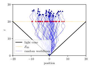
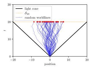
Figure 1: Random worldlines generated by eq.(28) (left) and eq.(29) (right)

The left picture in Fig.1 depicts 50 random worldlines generated by eq.(28) after a fixed “evolution time” $\tau=20$. The end point of each random worldline is marked by a solid triangle, and the horizontal line at $t=20$ represents the configuration space $\mathcal{S}_{20}$. We can see that all worldlines fall strictly in the future lightcone of the initial event $(t,x)=(0,0)$, and the end points of different random worldlines do not fall in the same configuration space. Nevertheless, we can extract the intersection point of each worldline with the configuration space $\mathcal{S}_{20}$ (marked with round dots) and try to identify their distribution.

The right picture in Fig.1 depicts 50 random worldlines generated by eq.(29) after the fixed evolution time $t=20$. Since $t$ is the regular evolution parameter, the end points of all worldlines automatically fall in the same configuration space $\mathcal{S}_{20}$ and are marked with round dots. This gives an intuitive illustration for the power of the reparametrization introduced in the last section. One can feel how similarly the round points in both pictures in Fig.1 are distributed.

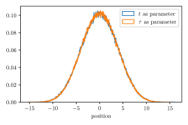
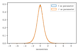
Figure 2: The distributions of Brownian particles in configuration space $\mathcal{S}_{20}$ (left) and momentum space (right) from the two systems of equations (28) and (29)

With a little more efforts, we have generated $10^{6}$ random phase trajectories using both eq.(28) and eq.(29) and collected the data for the insection points of the random worldlines with the configuration space $\mathcal{S}_{20}$ in the case of eq.(28). Using the data thus collected, we can depict separately the configuration space and momentum space distributions of the Brownian particles and make comparisons between the results that follow from eq.(28) and eq.(29). As can be seen in Fig.2, the results from eq.(28) and eq.(29) are almost identical.

We also generated the joint distributions in positions and momenta from both eqs.(28) and (29) at $t=20$. The results are presented in Fig.3. We can hardly find any differences between the two pictures.

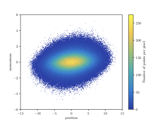
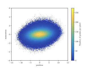
Figure 3: Joint probability distributions in positions and momenta at $t=20$: The left picture arises from eq.(28), and the right one arises from eq.(29). The distributions presented in Fig.2 correspond to vertical and horizontal projections of these joint distributions.

As a more serious comparison between the distributions generated by eqs.(28) and (29), the Pearson $\chi^{2}$-test is utilized with the assistance of Wolfram Language to determine whether the distributions were indeed identical. The resulting P-values were found to be $0.774$ for the distributions presented in the left plots of Fig.2, $0.967$ for distributions presented in the right plots of Fig.2, and $0.972$ for the two distributions presented in Fig.3. These results provide more solid evidence for the expectation that the distributions generated by the two systems of equations (28) and (29) are identical.

6 Concluding remarks

We have thus formulated two different versions of the relativistic Langevin equation, i.e. LE_τ and LE_t in a generic curved spacetime background, which are both manifestly general covariant. The two versions differ from each other in that LE_τ takes the proper time $\tau$ of the Brownian particle as evolution parameter, while LE_t takes the proper time $t$ of the prescribed observer Alice as evolution parameter.

The importance of the prescribed regularly moving observer is stressed throughout the analysis, especially while clarifying the SoMS of the Brownian particle and interpreting the probability distributions of the Brownian particle. It is argued that, in order to get the physical probability distribution, LE_t is more preferable than LE_τ. We also discussed the conditions which the relativistic damping coefficients need to obey, and clarified the concept of relative velocity in the relativistic context.

We also demonstrated, by means of Monte Carlo simulation in the particular example case of Brownian motion in $(1+1)$-dimensional Minkowski spacetime, that although LE_τ contains some conceptual issues, it is indeed possible to extract physically reasonable probability distributions from it. However, since the Brownian particles after a fixed proper time $\tau$ do not fall in the same configuration space, it would be more difficult to obtain the physical probability distributions from LE_τ.

This work is the first of our attempts for a systematic study of general relativistic stochastic mechanics. In a forthcoming work, we will proceed to formulate the corresponding Fokker-Planck equations and discuss the physical consequences. In particular, the general relativistic variant of Einstein relation will be considered, and the relationship between different probability distributions will be clarified.

Before ending this paper, let us mention that there is another complementary approach, i.e. the 2-jet bundle approach [31, 32] using Ito’s formalism, for describing the covariant Brownian motion [34, 35, 36, 37, 38], see also [39] for a more recent review. Our formalism does not need to make use of the jet bundle, and the resulting equations are more in line with the original intuitive construction of Langevin. There is some other recent work [40] which focuses on the heat distribution in Minkowski spacetime, which has some overlap in research subjects with the present work.

Data Availability Statement

All data used in this research was generated from eqs.(28) and (29) by use of numeric programs written in C++ and python. The P-values given in Sec.5 are calculated using Wolfram Language. All programs are available upon request.

Declaration of competing interest

The authors declare no competing interest.

References

- [1] Jüttner, F. “Das Maxwellsche Gesetz der Geschwindigkeitsverteilung in der Relativtheorie”, Ann. der Phys. 339, 856–882, 1911.
- [2] de Groot, S. R.; van Leeuwen, W. A.; van Weert, Ch. G. Relativistic Kinetic Theory: Principles and Applications. North-Holiand Publishing Company, 1980, ISBN: 9780444854537.
- [3] Cercignani, C; Kremer, G. M. The Relativistic Boltzmann Equation: Theory and Applications, volume 22. Springer Science & Business Media, 2002. ISBN: 9783034881654.
- [4] Vereshchagin, G. V.; Aksenov, A. G. Relativistic kinetic theory: with applications in astrophysics and cosmology. Cambridge University Press, 2017. ISBN: 9781107048225.
- [5] Acuña-Cárdenas, R. O.; Gabarrete, C.; Sarbach, O. “An introduction to the relativistic kinetic theory on curved spacetimes.” Gen. Rel. and Grav. 54(3): 1–120, 2022.[arXiv:2106.09235].
- [6] Debbasch, F.; Mallick, K.; Rivet, J. P. “Relativistic Ornstein–Uhlenbeck process,” J. Stat. Phys. 88(3): 945–966, 1997.
- [7] Debbasch, F. “A diffusion process in curved spacetime,” J. Math. Phys. 45(7): 2744–2760, 2004.
- [8] Dunkel, J.; Hänggi, P. “Theory of relativistic Brownian motion: the (1+1)-dimensional case.” Phys. Rev. E 71(1): 016124, 2005. [arXiv:cond-mat/0411011].
- [9] Dunkel, J.; Hänggi, P. “Theory of relativistic Brownian motion: The (1+ 3)-dimensional case,” Phys. Rev. E 72(3): 036106, 2005. [arXiv:cond-mat/0505532].
- [10] Fingerle, A. “Relativistic fluctuation theorems,” C. R. Phys. 8(5-6): 696–713, 2007. [arXiv:0705.3115].
- [11] Franchi, J.; Le Jan, Y. “Relativistic diffusions and Schwarzschild geometry,” Commun. Pure Appl. Math. 60(2): 187–251, 2007. [arXiv:math/0410485].
- [12] Dunkel, J.; Hänggi, P. “Relativistic Brownian motion,” Phys. Rep. 471(1): 1–73, 2009. [arXiv:0812.1996].
- [13] Dunkel, J.; Hänggi, P.; Weber, S. “Time parameters and Lorentz transformations of relativistic stochastic processes,” Phys. Rev. E 79(1): 010101, 2009. [arXiv:0812.0466].
- [14] Herrmann, J. “Diffusion in the special theory of relativity,” Phys. Rev. E 80(5): 051110, 2009.[arXiv:0903.0751].
- [15] Herrmann, J. “Diffusion in the general theory of relativity,” Phys. Rev. D 82(2): 024026, 2010. [arXiv:1003.3753].
- [16] Haba, Z. “Relativistic diffusion with friction on a pseudo-Riemannian manifold,” Class. Quant. Grav. 27(9): 095021, 2010. [arXiv:0909.2880].
- [17] Ding, M.; Tu, Z.; Xing, X. “Covariant formulation of nonlinear Langevin theory with multiplicative gaussian white noises,” Phys. Rev. Res. 2(3): 033381, 2020. [arXiv:2007.16131].
- [18] Ding, M.; Xing, X. “Covariant nonequilibrium thermodynamics from Ito-Langevin dynamics,” Phys. Rev. Res. 4(3): 033247, 2022.[arXiv:2105.14534v2].
- [19] Einstein, A. Eine neue bestimmung der moleküldimensionen, PhD thesis, ETH Zurich, 1905.
- [20] Einstein, A. “Über die von der molekularkinetischen theorie der wärme geforderte bewegung von in ruhenden flüssigkeiten suspendierten teilchen,” Ann. der Phys. 4, 1905.
- [21] Smoluchowski, M. “Zur kinetischen theorie der Brownschen molekular bewegung und der suspensionen,” Ann. der Phys. 21: 756–780, 1906.
- [22] Langevin, P. “Sur la théorie du mouvement Brownien,” C. R. Acad. Sci. 146: 530–533, 1908.
- [23] Ford, G. W.; Kac, M.; Mazur, P. “Statistical mechanics of assemblies of coupled oscillators,” J. Math. Phys. 6(4): 504–515, 1965.
- [24] Mori, H. “Transport, collective motion, and Brownian motion,” Prog. Theor. Phys. 33(3): 423–455, 1965.
- [25] Zwanzig, R. “Nonlinear generalized Langevin equations,” J. Stat. Phys. 9(3): 215–220, 1973.
- [26] Sekimoto, K. “Langevin equation and thermodynamics,” Prog. Theor. Phys. Supp. 130: 17–27, 1998.
- [27] Sekimoto, K. Stochastic energetics, volume 799. Springer, 2010. ISBN: 9783642054112.
- [28] Sarbach, O.; Zannias, T. “The geometry of the tangent bundle and the relativistic kinetic theory of gases,” Class. Quant. Grav. 31(8): 085013, 2014. [arXiv:1309.2036].
- [29] Gardiner, C. W. Handbook of stochastic methods for physics, chemistry and the natural sciences, volume 3. Springer Berlin, 1985. ISBN: 9783540208822.
- [30] Hsu, E. P. Stochastic analysis on manifolds, Number 38. American Mathematical Society, 2002. ISBN: 9780821808023.
- [31] Armstrong, J.; Brigo, D. “Coordinate-free stochastic differential equations as jets,” [arXiv:1602.03931].
- [32] Armstrong, J.; Brigo, D. “Intrinsic stochastic differential equations as jets,” Proceedings of the Royal Society A: Mathematical, Physical and Engineering Sciences, 474 (2210): 20170559, 2018.
- [33] Klimontovich, Y. L. “Nonlinear Brownian motion,” Phys-Usp, 37(8): 737, 1994.
- [34] Meyer, P. A. “A differential geometric formalism for the Itô calculus” Stochastic Integrals: Proceedings of the LMS Durham Symposium July 7-17, 1980, Springer Berlin, Heidelberg, 1981. ISBN: 9783540106906.
- [35] Schwartz, L. Semimartingales and their stochastic calculus on manifolds. Gaetan Morin Editeur Ltee, 1984. ISBN: 9782760606609.
- [36] Émery, M. Stochastic calculus in manifolds. Springer Science & Business Media, 2012. ISBN: 9783642750519.
- [37] Kuipers, F. “Stochastic quantization on lorentzian manifolds,” J. High Energ. Phys., 2021(5): 1–51, 2021. [arXiv:2101.12552].
- [38] Kuipers, F. “Stochastic quantization of relativistic theories,” J. Math. Phys., 62(12): 122301, 2021. [arXiv:2103.02501].
- [39] Kuipers, F. Stochastic Mechanics: The Unification of Quantum Mechanics with Brownian Motion. Springer Cham, 2023. ISBN: 9783031314476.
- [40] Paraguassu, P. V.; Morgado, W. A. M. “Heat distribution of relativistic Brownian motion,” Eur. Phys. J. B 94: 197, 2021.