End-of-Horizon Load Balancing Problems:
Algorithms and Insights

Abstract

Effective load balancing is at the heart of many applications in operations. Frequently tackled via the balls-into-bins paradigm, seminal results have shown that a limited amount of (costly) flexibility goes a long way in order to maintain (approximately) balanced loads throughout the decision-making horizon. This paper is motivated by the fact that balance across time is too stringent a requirement for some applications; rather, the only desideratum is approximate balance at the end of the horizon. Thus motivated, in this work we design “limited-flexibility” algorithms for three instantiations of the end-of-horizon balance problem: the canonical balls-into-bins problem [RS98], opaque selling strategies for inventory management, and parcel delivery for e-commerce fulfillment. For the balls-into-bins model, we show that a simple policy which begins exerting flexibility toward the end of the time horizon (i.e., when $\Theta\left(\sqrt{T\log T}\right)$ periods remain), suffices to achieve an approximately balanced load (i.e., a maximum load within $\mathcal{O}(1)$ of the average load). Moreover, with just a small amount of adaptivity, a threshold policy achieves the same result, while only exerting flexibility in $\mathcal{O}\left(\sqrt{T}\right)$ periods, thus matching a natural lower bound. We then adapt these algorithms to develop order-wise optimal policies for the opaque selling problem. Finally, we show via a data-driven case study on the 2021 Amazon Last Mile Routing Research Challenge that the adaptive policy designed for the simpler balls-into-bins model can be carefully modified to $(i)$ achieve approximate balance at the end of the horizon and $(ii)$ yield significant cost savings relative to policies which either never exert flexibility, or exert flexibility aggressively enough to always maintain balanced loads. The unifying motivation behind our algorithms for these three vastly different applications is the observation that exerting flexibility at the beginning of the horizon is likely wasted when system balance is only evaluated at the end.

1 Introduction

A key question in operations management is how to effectively address supply-demand imbalances. When a decision-maker has access to different supply sources, and these imbalances are only due to stochastic fluctuations, this question is often tackled through the lens of load balancing. The canonical model of load balancing is the balls-into-bins paradigm, in which balls (demand) are sequentially placed into bins (supply) according to some (potentially random) allocation scheme. These models are used to understand how a decision-maker can maintain a (approximately) balanced load across bins over time, i.e., design policies that keep the number of balls in each bin approximately equal. This is a natural goal in many applications, including queuing settings where average delay is a metric of interest. In many other applications, however, maintaining a balanced load over all time may be an unnecessarily stringent requirement. Instead, there may only be specific points in time at which balance is required, or even a single such point. This point in time may be a priori unknown, it may depend on the way in which the process unfolds, and it may depend on the decision-maker’s previous actions. Examples where this is the case include the following:

GPU management in cloud computing. Consider an incoming stream of data that must be instantaneously allocated to a set of servers. Since GPU time on servers is expensive, these servers only start processing the files once they have all been received [Ell15]. In order to minimize the makespan of the processing time, it is beneficial to have the workload be as balanced as possible across the servers once all files have been received; however, at intermediate points before the stream ends, balance across servers is not a metric of interest.

Inventory management. Consider a retailer that sells a large number of a few different products, and jointly restocks them all once the stock of any one product is depleted. For inventory costs to be minimized, the retailer wants all items to be close to depletion at the time when restocking occurs (see Section 2 for more details); however, imbalances in remaining inventory do not affect the retailer’s supply costs at other points in time [EYZ19].

Parcel delivery. Consider a delivery fulfillment center in which parcels arrive in an online fashion over the course of a day. When a parcel arrives, it is allocated to one of several different trucks based on its destination. To avoid some trucks being overutilized, the goal is to have different trucks with approximately equal loads. However, for the truck’s utilization only the final load matters; at earlier times during the day the balance of parcels is immaterial for the later truck utilization.

Common to these three examples is that, rather than aiming to keep the system balanced throughout time, a decision-maker (DM) only requires balance at a single point in time, a goal that is potentially much easier to achieve. In this work we aim to investigate to what extent this can reduce the cost of the DM’s operations. Loosely speaking, we consider settings of the following form: in each period an arrival occurs, and the DM needs to decide whether or not to exert flexibility. If she does, there is a constant probability that she gets to decide in which bin, out of a subset of randomly sampled bins, to place the arrival. Otherwise, the arrival is placed in a bin chosen uniformly at random. [PTW10] showed that exerting flexibility in every period allows the DM to keep the load approximately balanced — i.e., the deviation between the maximum and average loads across bins is upper bounded by a constant independent of the time horizon — at all times with high probability. Against this backdrop, this work considers the following question: Can a DM achieve the less ambitious goal of balance at the end of the time horizon while exerting significantly less flexibility?

1.1 Our contributions

We study three instantiations of this problem with varying levels of complexity. The first — and most tractable — of these is a “limited-flexibility” variant of the canonical balls-into-bins model studied in the applied probability and theoretical computer science communities. We leverage our analysis of this vanilla framework when we subsequently consider the problem of designing (near)-optimal opaque selling strategies for inventory management. Finally, we adapt these policies to the significantly more complex problem of parcel delivery in e-commerce fulfillment, demonstrating their practical use via a data-driven case study.

Vanilla balls-into-bins.

For the standard balls-into-bins problem, we design two policies that achieve approximate balance at the end of a time horizon of length $T$ with limited flexibility. The first is a non-adaptive policy — which we term the static policy — that starts exerting flexibility when $\Theta\left(\sqrt{T\log T}\right)$ periods remain in the time horizon. We show that such a policy can approximately achieve balance at the end of the time horizon while exerting flexibility only $\Theta\left(\sqrt{T\log T}\right)$ times, whereas any policy that achieves approximate balance requires exerting flexibility $\Omega\left(\sqrt{T}\right)$ times in expectation. We further show that no policy that starts exerting flexibility at a deterministic point in time can close this gap to $\Theta\left(\sqrt{T}\right)$. Motivated by this fact, we design a dynamic policy to match this lower bound. This policy exerts flexibility whenever the imbalance of the system exceeds a carefully designed, time-varying threshold.

The analysis of this first problem is based on the following main idea: over the course of the entire time horizon, if the decision-maker never exerted flexibility, the imbalance between bins would scale as $\Theta\left(\sqrt{T}\right)$. If each time the decision-maker exerted flexibility that imbalance was reduced by $1$, then she would only need to do so $\mathcal{O}\left(\sqrt{T}\right)$ times in order to achieve approximate balance. Though exerting flexibility always reduces the instantaneous imbalance among the bins, it does not always reduce the imbalance as measured in hindsight. For instance, suppose the decision-maker exerted flexibility early on during the time horizon to put a ball into bin $i$ that would have landed in bin $j$ in the absence of flexibility; if it turned out in hindsight that more balls landed in bin $i$ than in bin $j$, then exerting flexibility in this early period (keeping all later decisions fixed) would actually increase, not decrease, the imbalance over the entire horizon. However, if she only starts exerting flexibility towards the end of the horizon, when the imbalance is of size $\Theta\left(\sqrt{T}\right)$ and only $o(T)$ periods remain, then it is unlikely that the imbalance between $i$ and $j$ would be overcome by the natural variation of the stochastic process, and consequently exerting flexibility is likely to reduce the imbalance as measured over the entire horizon. On a technical level, our analysis requires us to overcome a number of hurdles in analyzing non-trivial stochastic processes. The main difficulty stems from the fact that the system is already imbalanced when the decision-maker first exerts flexibility; as a result, a good policy must ensure the flexibility exerted in the remaining rounds suffices to close this existing gap. This difficulty is compounded in the analysis of our dynamic policy for which flexing commences at a random time. Thus, designing such an adaptive policy requires us to construct the threshold carefully enough that the now-random number of rounds remaining suffices to control the accumulated imbalance.

Opaque Selling.

We subsequently turn our attention to the problem of opaque selling in inventory management. In this setting, to ensure that inventory isn’t replenished too frequently, a retailer can exert flexibility by offering a discounted opaque option to customers. Under this practice the customer chooses a subset of items, and the retailer decides which item from this subset is sold to the customer. To minimize total inventory and discount costs, the retailer must trade off between the benefits of increasing (expected) time-to-replenishment (i.e., minimizing the imbalance of inventory levels across items), and the cost of offering the discounted option to achieve this outcome. The additional level of complexity in this setting is that, in contrast to the known and deterministic time horizon in the balls-into-bins problem, the time horizon corresponds to the (random) first time a product is depleted, which depends on both the random realization of arrivals and the DM’s actions. The introduction of this moving target requires the DM to exert flexibility more frequently than the dynamic policy designed for balls-into-bins; to address this we design a semi-dynamic policy which similarly maintains a time-varying threshold on the imbalance of the inventory level, and offers the opaque option starting from the first time the imbalance condition is triggered, all the way to the time of depletion. We show that in a large-inventory scaling the per-period loss of the semi-dynamic policy converges, for a range of parameter regimes, at a linear rate to a loose lower bound in which the DM’s inventory is depleted evenly without the DM ever needing to exert flexibility. For parameters where this is not the case, its loss relative to that lower bound is of the same/better order as that of natural benchmark “never-flex” and “always-flex” policies (which, as the names indicate, respectively never exert the flexible option, or do so in every time period). We complement our theoretical results with synthetic experiments that demonstrate the robustness of our insights with respect to $(i)$ different input parameters and $(ii)$ varying threshold choices for our algorithms.

Parcel delivery in e-commerce fulfillment.

We finally consider the problem of parcel delivery in e-commerce fulfillment. In the setting we consider, a warehouse receives a sequence of packages throughout the day, and must assign each package to one of $N$ trucks in online fashion. The goal is to find an assignment of packages to trucks that minimizes expected routing costs and overtime pay to delivery drivers. As is common in practice, packages are ex-ante associated with default trucks based on their geographic coordinates [CLSY21]. However, given the fluctuation of volumes in each region across days, it may be desirable to exert flexibility by assigning packages to non-default trucks. This flexibility, however, comes at a cost, as a non-default assignment may cause costly detours in hindsight. Though this problem bears conceptual similarities to the balls-into-bins and inventory management models we consider for our analytical results, the routing component adds a significant level of complexity. Indeed, the offline setting generalizes the Travelling Salesman Problem, given the overtime pay consideration. In the online setting, a good flexing policy must also contend with the fact that “mistakes” due to flexing may be much costlier in hindsight than in the two previously studied settings. Still, we show via a case study on the 2021 Amazon Last Mile Routing Research Challenge Dataset [MAP⁺22] that a careful adaptation of the balls-into-bins dynamic policy yields on the order of 5% cost savings relative to the default-only, “no-flex” policy.

In summary, our work explores load-balancing applications in which balance is evaluated not across periods, but only at a specific point in time. For these scenarios, common in both analogue and digital applications, we design simple heuristics that combine three attractive properties: $(i)$ provable approximate balance at the end of the horizon, $(ii)$ a significantly lower need to exert flexibility when compared to standard approaches that guarantee balance throughout, and $(iii)$ adaptability to vastly different contexts. The unifying motivation for these heuristics is the observation that exerting flexibility at the beginning of a horizon is likely wasted/unnecessary when system balance is only evaluated at the end.

1.2 Related work

Our work relates to three traditional streams of literature: work on the balls-into-bins model, revenue management literature related to opaque selling (and more generally, the value of demand flexibility in service systems), and vehicle routing as it relates to parcel delivery. We survey the most closely related papers for each of these lines of work below.

The balls-into-bins model. As noted above, the balls-into-bins model has a long history in the theoretical computer science literature, with a number of variants proposed and used to model a variety of computing applications. We refer the reader to [RMS01] for an exhaustive survey, and only highlight two closely related results: [RS98] consider the basic model in which balls are sequentially (and randomly) thrown into $n$ bins, and derive sharp upper and lower high-probability bounds on the maximum number of balls in any bin after $m$ throws, finding that the gap between the maximally loaded bin and the average load is $\Theta\left(\sqrt{\frac{m\log n}{n}}\right)$. Later, [PTW10] showed that, if the ball goes into a random bin with probability $q$, and the lesser-loaded of two random bins with probability $1-q$, this expected gap is a constant independent of $m$ (though dependent on the number of bins $n$). We leverage these latter results in the analyses of the policies we consider for both the balls-into-bins and the opaque selling problem.

On the power of flexibility in opaque selling. The practice of offering opaque, or flexible, products to customers has long been studied in operations management. In particular, it has been found that opaque selling has two potential benefits, from a revenue perspective: $(i)$ it may increase the overall demand for products, and $(ii)$ it may enable better capacity utilization when there is a mismatch between capacity and demand [GP04]. In this regard, there has been growing attention regarding how one can leverage opaque selling to price discriminate among customers who are differentiated in their willingness to pay for products [Jia07, FX08, JNV09, EH21]. These papers all focus on the retailer’s pricing decisions, rather than the inventory management problem which we consider here.

More recently the literature has formalized the inventory cost savings that can be realized due to the flexibility of customers who pick opaque options. [XC14] consider a simple model in which a retailer sells two similar products over a finite selling period, and quantify the potential inventory pooling effect of opaque selling for this stylized model. [EWZ15] similarly consider a two-product model with replenishments, and analytically show that selling relatively few opaque products to balance inventory can have substantial cost advantages. [EYZ19], to which our work is most closely related, generalize this latter model to $N$ products and makes, to the best of our knowledge, the first connection to the seminal balls-into-bins model. Our work relates to this latter paper in that we show that one need not exercise the opaque option with every flexible customer to realize the full benefits of opaque selling: strategically timed end-of-season opaque promotions suffice.

General flexible processes. The idea of inventory cost savings from opaque selling is closely related to other recent studies that consider how demand-side flexibility can improve supply costs/utilization. [ELZ21] and [FvR21] respectively consider (time-)flexible demand in scheduled service systems and ride-hailing, and demonstrate how flexibility improves utilization for these. Relatedly, [GY21] show the value of demand flexibility in a resource allocation setting in which both time-flexible and time-inflexible customers seek a service with periodic replenishments. [ZT22] consider a flexible variant of the classical network revenue management problem, in which a service provider gets to choose which combination of resources is used to serve each customer. Contrary to our setting, however, the act of exerting flexibility does not come at an extra cost. Finally, closely related to our case study, [DWWY21] consider a model in which an online retailer can fulfill customer demand in two ways: either from a nearby, “local” distribution center, or from a distribution center that is further away, and poses the risk of customer abandonment due to longer delivery times. Whereas they assume a constant cost of assignment to each distribution center, we are interested in the micro-level truck assignment and routing policies induced by the flexible policy, which adds significant complexity to the problem.

We note that characterizing the power of flexibility has a long history in both the theoretical computer science and the operations literature: the seminal works of [ABKU94] and [Mit96] (load balancing), [TX13] and [TX17] (resource pooling), as well as [JG95] (manufacturing) are perhaps the most notable examples of these respective streams of work. All of these demonstrate that small amounts of flexibility suffice to realize most of the benefits of full flexibility. For an overview of more recent results on flexibility in the operations literature, [WWZ21] provides an excellent survey.

Vehicle routing. The dataset we use for our case study originates from the 2021 Amazon Last Mile Routing Research Challenge [MAP⁺22], whose aim it was to encourage data-driven and learning-based solution approaches that mimic existing high-quality routes operated by experienced drivers, after the assignment of packages to trucks. In contrast, we are interested in the problem that precedes this (i.e., the assignment itself), which renders solutions proposed for the competition (e.g., [CHH22]), as well as case studies on single-vehicle routing heuristics that rely on the dataset [RZ23] tangent to our problem.

The problem we consider for this setting is closely related to the Vehicle Routing Problem (VRP) [GRW⁺08, TV14, MS22], and more specifically the online multiple-vehicle routing problem (see [JW08] for an excellent survey). Though we also consider a variant of online VRP, a key difference of our model is that we also account for the cost of overtime wages (in addition to travel time), thus placing a premium on balanced loads. This is in a similar spirit to prior work that aims for an even partition of workload [HHL07, CD13b, CD13a]. These works, however, focus on optimal partitioning of the service territory into sub-regions and require that each vehicle only be responsible for demand occurring in its own sub-region. In contrast, we are interested in the value of (infrequently) violating this partitioning. More importantly, we highlight that the goal of our case study is not to propose new algorithms for the online vehicle routing problem, or its applications in parcel delivery. Instead, we aim to leverage our load balancing insights to show that reasonable heuristics that exert flexibility sparingly can yield significant cost savings.

2 Basic Setup

In this section we present the classical balls-into-bins model [Mit01, PTW10], which also forms the backbone of the applications we study.

The vanilla balls-into-bins model evolves over a discrete, finite-time horizon in which $T$ balls are sequentially allocated into $N\geq 2$ bins. Each ball is a flex ball with probability $q\in(0,1]$. If a ball is a flex ball, the decision-maker (DM) may exert flexibility; if she exercises this flexibility, she observes a set of size $r$ — the flex set $F(t)$ — drawn uniformly at random from $\{1,2,...,N\}$, and chooses the bin in $F(t)$ to which the ball is allocated. If a ball is not a flex ball, we write $F(t)=\phi$. Such a ball, or one for which the flexibility is not exerted, is placed into a bin drawn uniformly at random, denoted by $P(t)$. We let $f(t)$ be the indicator variable that denotes whether the ball is flexible, with $f(t)=1$ if it is, and $f(t)=0$ otherwise. Note that $f(t)\sim\textup{Ber}(q)$. The type $\theta({t}){=\left(f(t),P(t),F(t)\right)}$ of a ball at time $t\in\{1,2,...,T\}$ is characterized by $(i)$ whether or not it is a flex ball, $(ii)$ the bin it would go into without flexibility, and $(iii)$ the ball’s flex set. We further define the history of balls $\sigma(t)$ to be the types of all balls before time $t$, i.e., $\sigma(t)=(\theta({1}),\ldots,\theta({t-1})),$ and let $\Sigma(t)$ be the set of all possible histories at time $t$.

The DM’s policy $\pi$ is characterized by a tuple consisting of both the decision to exercise the flex throw, denoted by $\omega^{\pi}(t)$ (with $\omega^{\pi}(t)=1$ if exercised, and 0 otherwise), and which bin to throw the ball into, denoted by $\mathcal{A}^{\pi}(t)$. With $x_{i}^{\pi}(t)$ denoting the number of balls in bin $i$ at the beginning of period $t$, the second decision is assumed to be, unless otherwise specified,

$$\mathcal{A}^{\pi}(t)=\begin{cases}\arg\min_{j\in F(t)}x_{j}^{\pi}(t)&\quad\text{if }f(t)\omega(t)=1,\\ P(t)&\quad\text{if }f(t)\omega(t)=0.\end{cases}$$

Here, we define the $\arg\min$ with a lexicographic tie-breaking rule that returns the smallest value $i$ of all bins with the smallest number of balls.

The DM’s goal is to ensure that the load across bins (i.e., the number of balls in each bin) is approximately balanced at the end of the time horizon. To characterize the degree of imbalance of the state of the system at time $t$, we define the gap of the system under $\pi$ as the difference between the maximum load across all bins and the average load. Note that, given $t\in\mathbb{N}^{+}$, the average load is given by $t/N$, since exactly one ball is thrown in each period. Then, for policy $\pi$, we denote:

$$Gap^{\pi}(t)=\max_{i\in[N]}x_{i}^{\pi}(t)-\frac{t}{N}\quad\forall\,t\in\mathbb{N}^{+}.$$

The DM’s goal is to design a policy $\pi$ such that $\mathbb{E}\left[Gap^{\pi}\left(T\right)\right]\in\mathcal{O}(1)$, where the Big-O notation is with respect to the time horizon $T$. If this is satisfied under $\pi$, we say that the system is approximately balanced. We further let $M^{\pi}$ denote the number of times that the decision-maker gets to choose the bin that a flex ball goes into. Formally, $M^{\pi}=\sum_{t=1}^{T}f_{B}(t)\omega_{B}(t).$

Benchmarks.

In order to contextualize the performance of our policies, we present two simple policies that have previously been analyzed in the literature. The no-flex policy, denoted by superscript $nf,$ sets $\omega^{nf}(t)=0\;\forall\ t.$ By construction, the no-flex policy yields $M^{nf}=0$, but a gap that grows with the horizon $\mathbb{E}\left[Gap^{nf}\right]\in\Theta\left(\sqrt{T}\right)$ [RS98]. On the other hand, the always-flex policy, denoted by superscript $a,$ sets $\omega^{a}(t)=~{}1\;\forall t$. This leads to $\mathbb{E}\left[M^{a}\right]{=Tq}$ with a balanced load at $T$ (i.e., $\mathbb{E}\left[Gap^{a}\right]\in\mathcal{O}(1)$, by [PTW10]).

Remark 1.

We assume without loss of generality that our policies operate with $r=2$, i.e., we have $|F(t)|=2\ \forall\ t$. Our algorithms can be directly adapted to arbitrary $r$ as follows: when $|F(t)|>2$, choose a subset of size 2 of $F(t)$ uniformly at random, and flex only within this subset. Hence, we abuse notation by writing our policies for arbitrary flex sets, but analyze them for $r=2$.

3 Analytical Results

In this section, we propose and analyze two policies that achieve two desiderata for the balls-into-bins problem: $(i)$ keeping the load approximately balanced at the end of the time horizon, and $(ii)$ doing this with as few flexes as possible (e.g., $o(T)$ flexes). We then show how these algorithms can be leveraged within the context of inventory management.

Before presenting our two policies, we first turn to the question of how many flexes are required to achieve an approximately balanced system. Proposition 1 establishes a lower bound.

Proposition 1.

Consider any policy $\pi$ such that $\mathbb{E}\left[Gap^{\pi}(T)\right]\in\mathcal{O}(1)$. Then, $\mathbb{E}\left[M^{\pi}\right]\in\Omega\left(\sqrt{T}\right).$

This lower bound is quite intuitive: every time the DM exerts flexibility, the gap at time $T$ decreases by at most 1. Since the expected gap when balls are randomly thrown into the bins is well-known to scale as $\Theta\left(\sqrt{T}\right)$, closing this gap to $\mathcal{O}(1)$ would require the decision-maker to exert flexibility at least $\Theta\left(\sqrt{T}\right)$ times. We defer a full proof to Appendix A.1.2.

We next design two policies that strive to achieve this lower bound. Both leverage the fact that, without any flexing, the load in each bin at the end of the time horizon is, with high probability, within $\Theta\left(\sqrt{T}\right)$ of the expected load $T/N$. Thus, it should suffice to begin exercising the flex option with $\widetilde{\mathcal{O}}\left(\sqrt{T}\right)$ periods remaining.

The first policy we consider, referred to as the static policy $\pi^{s}$, is non-adaptive, and exerts flexibility if and only if $\Theta\left(\sqrt{T\log T}\right)$ periods remain. Specifically, $\pi^{s}$ fixes a time $\widehat{T}=T-a_{{s}}\sqrt{T\log T}$, where $a_{{s}}=\frac{2\sqrt{6}N(N-1)}{q}$. It begins actively load balancing, placing flex balls in the minimally loaded bin within the flex set for all $t\geq\widehat{T}$, but not before (see Algorithm 3 in Appendix A.1.1).

With $Gap^{s}(t)$ denoting the gap in period $t$ for the static policy, we now establish that the intuition underlying the design of this naive policy is correct: exerting flexibility $\Theta(\sqrt{T\log T})$ times suffices to achieve a balanced load by the end of the horizon (proof in Appendix A.1.4).

Theorem 1.

For the static policy defined in Algorithm 3, $\mathbb{E}\left[Gap^{s}(T)\right]\in\mathcal{O}\left(1\right).$

We highlight that this result holds for arbitrary $r\in\left\{2,\ldots,N\right\}$. Thus, a slight subtlety in establishing this result is that, for $r<N$, balls are not always allocated to the minimally loaded bin; exerting a flex may then in theory increase the gap of the system. However, we show that starting to flex $\Theta(\sqrt{T\log T})$ periods before the end of the horizon precludes these “errors” from occurring too frequently in expectation, and we are nonetheless able to achieve a constant gap.

Our static policy does not exactly meet the lower bound from Proposition 1 due to the additional $\mathcal{O}\left(\sqrt{\log T}\right)$ factor. This is not an artifact of our analysis, nor is it due to our definition of $a_{{s}}$. Instead, it is a general fact about non-adaptive policies: no non-adaptive policy can achieve $\mathcal{O}(1)$ gap at $T$ while exerting flexibility $\mathcal{O}\left(\sqrt{T}\right)$ times (see Proposition 2 in Appendix A.1.3).

3.1 The Dynamic Policy

The static policy proposed above ignores the fact that not all sample paths are created equal — while the loads under certain sample paths require a larger number of flexes to achieve balance, on others a smaller number suffices. Thus, although Proposition 2 implies that no static policy can achieve an approximately balanced load with $\mathcal{O}\left(\sqrt{T}\right)$ flexes, it may be that an adaptive policy can.

We thus consider an adaptive policy, referred to as the dynamic policy, which flexes only when the gap of the system exceeds (a constant factor of) the expected remaining number of flexes. Periods in which this condition is satisfied can be viewed as a “point of no return”; since exerting a flex in any given period reduces the gap of the system by at most one, if the current gap exceeds the remaining number of flex balls by a significant amount, then there is no hope obtaining a balanced load at the end of the horizon. We provide a formal description of the dynamic policy in Algorithm 1, with superscript d referring to quantities induced by the dynamic policy.

Algorithm 1 Dynamic Policy $\pi^{d}$

1:Initialize $x^{d}_{i}(0)=0\;\forall\,i\in[N]$, $a_{{d}}=\frac{1}{5\binom{N}{2}}$, $\omega(t)=0\;\forall t$ 

2:for $t\in[T]$ do

3:     if $Gap^{d}(t)\geq\frac{a_{{d}}(T-t)q}{N}$ then

4:         $\omega(t)=1$

5:     end if

6:     if $\omega(t)f(t)=1$ then

7:         $\mathcal{A}^{d}(t)=\operatorname*{arg\,min}_{i\in F(t)}x^{d}_{i}(t)$

8:     else $\mathcal{A}^{d}(t)=P(t)$

9:     end if

10:     for $i\in[N]$ do

11:         $x^{d}_{i}(t+1)=\begin{cases}x^{d}_{i}(t)+1&\quad\text{if }i=\mathcal{A}^{d}(t)\\ x^{d}_{i}(t)&\quad\text{otherwise}.\end{cases}$

12:     end for

13:end for

The following two theorems establish that such a “point of no return”-type policy meets both desiderata: a constant gap at time $T$ with $\mathcal{O}\left(\sqrt{T}\right)$ balls flexibly allocated in expectation.

Theorem 2.

For the dynamic policy defined in Algorithm 1, $\mathbb{E}\left[Gap^{d}(T)\right]\in\mathcal{O}(1).$

Theorem 3.

For any constant $a>0,$ let $T_{a}:=\inf\left\{t:Gap^{nf}(t)\geq\frac{a(T-t)q}{N}\right\}$. Then, $\mathbb{E}[T-T_{a}]\in\mathcal{O}\left(\sqrt{T}\right).$ Thus, the dynamic policy achieves $\mathbb{E}\left[M^{d}\right]\in\mathcal{O}\left(\sqrt{T}\right)$.

We first provide some high-level intuition for Theorem 3, deferring its proof to Appendix A.2.2. Consider the first time the flexing condition is triggered, denoted by $t^{\text{start}}$. Since the dynamic policy makes the same decisions as the no-flex policy before $t^{\text{start}}$, we have $Gap^{d}(t^{\text{start}})\in\mathcal{O}(\sqrt{t^{\text{start}}})$ with high probability [RS98]. Solving the flexing condition for $t^{\text{start}}$ we obtain an approximate high-probability upper bound of $t^{\text{start}}=T-\mathcal{O}(\sqrt{T})$. Since the number of flexes exerted by the dynamic policy is upper bounded by $T-t^{\text{start}}$, this yields a high-probability upper bound on the expected number of flexes. Translating this intuition into a formal proof, however, presents additional challenges, including the fact that large-deviation bounds on the binomial distribution are too loose to yield the desired result, and thus require tighter bounds on $t^{\text{start}}$.

In contrast to the static policy, which begins flexing aggressively within ${\Theta}(\sqrt{T\log T})$ periods of the end of the time horizon, the key challenge in analyzing the dynamic policy is that it exerts flexibility only when absolutely necessary, i.e., at the point of no return described above. Indeed, it is not immediately clear that such parsimony suffices to recoup the imbalance accumulated before the first time the threshold was satisfied. We however leverage the construction of the adaptive threshold to show that the gap accumulated whenever $\pi^{d}$ isn’t flexing can be reduced to a constant in expectation by being progressively more aggressive as the end of the horizon approaches. We defer the formal proof of Theorem 2 to Appendix A.2.1, and provide a proof sketch below.

Proof sketch of Theorem 2.

The proof upper bounds the gap at time $T$ by conditioning on a particular pair of bins $i$ and $j$ to respectively be the most- and least-filled bins at that time. It then defines $T^{\star}$ as the start of the last consecutive sequence of periods in which the dynamic policy always exerts flexibility, and considers two events: either bins $i$ and $j$ never have the same load in the periods $T^{\star},\ldots,T$ or they do.

Consider first the event that bins $i$ and $j$ have the same load in some period $t\in\{T^{\star},\ldots,T\}$, and let $\tau$ denote the last period in which this occurs. We observe that $T-\tau$ is an upper bound on the gap at time $T$. We then establish that $T-\tau$ is unlikely to be large, which follows from the following three facts: $(i)$ bins $i$ and $j$ have the same load in period $\tau$, $(ii)$ the policy always exerts flexibility between $\tau$ and $T$, and $(iii)$ $i$ has larger load than $j$ between $\tau+1$ and $T$ (since $i$ is defined to be the most-loaded bin at $T$). As a result, the policy biases balls away from $i$ and toward $j$, thus pushing the difference in loads between the two bins toward 0. The formal analysis of this event requires us to define a fictitious state-independent policy that allows us to bound probabilities without the pitfalls of the conditional probabilities induced by the case analysis.

Consider now the event that $i$ and $j$ never have the same load in any period between $T^{\star}$ and $T$. We similarly condition on the value of $T-T^{\star}$, noting that $(i)$ the definition of $T^{\star}$ gives an upper bound on the gap at time $T^{\star}$ (namely, $Gap^{d}(T^{\star})\approx\frac{a_{d}(T-T^{\star})q}{N}$) and $(ii)$ the gap increases by at most $T-T^{\star}$ between $T^{\star}$ and $T$. As a result, it suffices to probabilistically bound $T-T^{\star}$; similar to the above, we obtain this bound by observing that the policy biases decisions away from $i$ and toward $j$. Given this, for $i$ to maintain a larger load than $j$ over periods $T^{\star},\ldots,T$ it cannot be the case that $T-T^{\star}$ is too large. Here as well, the devil is in the details as the formal proof requires us to circumvent dealing with the conditional probabilities induced by the case analysis.

3.2 Application: Inventory Management and Opaque Selling

We now leverage the results obtained for the balls-into-bins model to derive insights into the design of policies for the opaque selling problem. We first present the opaque selling model, similar to that of [EYZ19] who previously observed the analogy between the two models.

Customers.

A retailer sells $N\geq 2$ horizontally differentiated (i.e., identical from a quality perspective), equally-priced product types to customers over an infinite horizon. In each period, a customer arrives seeking to buy her preferred item at the regular price, which is normalized to 1. In addition to the regular-priced option, the retailer may offer an opaque promotion wherein the customer may pick a subset of items of size $r\leq N$ — the flex set — and receive an additive discount $\delta\in(0,1)$. The retailer then sells the item in the flex set for which the most inventory remains. Motivated by the fact that products are horizontally differentiated, we assume that a customer draws both her preferred item and the flex set uniformly at random.

Inventory dynamics.

The retailer begins with $S$ units of inventory for each item at $t=0$. In each period, the retailer incurs a holding cost $h\in\mathbb{R}_{>0}$ per unit of inventory on-hand. Whenever the inventory level of a product drops to 0, the stock of all $N$ products is immediately replenished to the initial inventory level $S$ at a joint replenishment cost $K\in\mathbb{R}_{>0}$ [Har90], and refer to the amount of time between two consecutive inventory replenishments as a replenishment cycle.

Retailer policy and objective.

The goal of the retailer is to find a policy $\pi$ — which determines whether or not to offer the opaque option to a customer in each period — that minimizes her long-run average inventory costs, composed of holding costs, replenishment costs, and discount costs. As derived in [EYZ19], this long-run average objective is given by:

$$\mathcal{C}^{\pi} =\frac{K}{\mathbb{E}\left[R^{\pi}\right]}+\frac{h}{2}\left(2NS+1-\frac{\mathbb{E}\left[(R^{\pi})^{2}\right]}{\mathbb{E}\left[R^{\pi}\right]}\right)+\frac{\mathbb{E}\left[D^{\pi}\right]}{\mathbb{E}\left[R^{\pi}\right]}\,\delta.$$ (1)

Analogy to balls-into-bins and results.

The analogy is as follows: bins correspond to products, and balls to customers. Specifically, one can view a customer purchasing a given product (and depleting the product’s inventory by one) as a ball being allocated to a bin (and increasing the bin’s load by one). With this analogy, a “good” policy trades off between exercising the opaque option often enough to keep inventory levels approximately balanced, thus ensuring long replenishment cycles, but not so often that its discount costs are too high.

Despite the straightforward analogy between the two models, there exist a subtle — yet important — difference that presents an additional challenge in designing and analyzing policies for the opaque selling model. In particular, contrary to the balls-into-bins model, in the opaque selling problem not only is the end of the time horizon (i.e., the length of the replenishment cycle) unknown, but it also depends on the time at which the policy begins flexing. As a result, policies that start flexing a fixed number of periods before the horizon ends are not implementable. This renders adaptive policies, which exert flexibility based on inventory state, particularly attractive. We thus consider a variant of the dynamic policy previously proposed. To do so, we define

$$Gap_{I}^{\pi}(t)=S-\min_{i\in[N]}z_{i}^{\pi}(t)-\frac{t}{N},\quad\forall\,t\in[R^{\pi}],$$ (2)

where $z_{i}^{\pi}(t)\in[1,S]$ denotes the remaining inventory of item $i$ in period $t$ under policy $\pi$, $R^{\pi}$ is the replenishment cycle in which $t$ finds itself, and $t$ is re-initialized every time the retailer’s inventory is replenished. Under the dynamic opaque selling policy, denoted again by $\pi^{d}$, the DM starts exercising the opaque option the first time the gap (weakly) exceeds $\frac{c_{d}(T-t)q}{N}$, where $c_{d}=\frac{1}{10\binom{N}{2}}$. From then on, $\pi^{d}$ sells the product with the most remaining inventory in the customer’s flex set.

We benchmark the cost $\mathcal{C}^{d}$ incurred by $\pi^{d}$ against $(i)$ $\mathcal{C}^{nf}$, the cost of the “never-flex” policy, which never exercises the opaque option, $(ii)$ $\mathcal{C}^{a}$, that of the “always-flex” policy, which exercises the opaque option whenever the customer is open to flexing, $(iii)$ $\mathcal{C}^{s}$, that of a static policy, which begins exercising the opaque option in period $T-c_{s}\sqrt{T\log T}$ for some $c_{s}>0$, where $T:=N(S-1)+1$ is a loose upper bound on the length of any replenishment cycle, and $(iv)$ a lower bound $\mathcal{C}^{\star}=\frac{K}{N(S-1)+1}+\frac{h}{2}(NS+N)$ on the least possible long-run average cost.

Our main result for this section considers a “large-inventory” limit in which $S$ grows large, with $K\in\Theta(S)$ and $h\in\Theta\left(\frac{1}{S}\right)$ (i.e., the per-unit replenishment and average holding cost are both $\Theta(1)$).

Theorem 4.

Suppose $K\in\Theta(S)$ and $h\in\Theta\left(\frac{1}{S}\right)$. Then, the following holds:

1. When $\delta\in\mathcal{O}\left(\frac{1}{\sqrt{S}}\right)$, $\mathcal{C}^{d}-\mathcal{C}^{\star}\leq\mathcal{O}\left(\frac{1}{S}\right),$ i.e., the dynamic policy is optimal up to a constant additive loss in each replenishment cycle.

2. When $\delta\in\Omega\left(\frac{1}{\sqrt{S}}\right)$ and $\delta\in\mathcal{O}(1)$, of the four policies, the dynamic policy has the order-wise best performance relative to $\mathcal{C}^{\star}$.

Theorem 4 guarantees that, as long as the cost of each opaque promotion is not overwhelmingly high (i.e., as long as $\delta\in\mathcal{O}(1)$), the dynamic policy (order-wise) performs best among the four policies. If, moreover, the promotional cost is relatively small as compared with the inventory cost (i.e., $\delta\in\mathcal{O}\left(\frac{1}{\sqrt{S}}\right)$), the dynamic policy incurs at most a constant loss relative to the universal lower bound $\mathcal{C}^{\star}$ in each replenishment cycle, even as $S$ scales large.

The proof of Theorem 4 relies on tight analyses of the expected cycle length of the dynamic and benchmark policies which require bounds on the tail of the distribution of the gap of the system, rather than the expected gap, in contrast to the vanilla balls-into-bins model we analyzed above. We defer its lengthy proof to Appendix B.

Numerical results.

We next numerically investigate the performance of our policies in the opaque selling model. In the remainder of this section, we refer to the difference between maximum and expected replenishment cycle length (i.e., $T-\mathbb{E}\left[R^{\pi}\right]$) as system balancedness.

Inputs.

Unless otherwise stated, our numerical results assume $N=5$, $q=0.1$ and $r=2$. We instantiate the static and dynamic policies with $a_{{s}}=10$ and $a_{{d}}=0.7$, respectively (see Appendix B.6 for experiments on robustness of our results to these hyperparameters). We simulate the long-run average performance of each tested policy over $10$ instances of $10$ replenishment cycles.

Benchmark comparisons.

Beyond the four policies (no-flex, always-flex, static and dynamic) studied above, we consider an additional benchmark policy, the flex-$\sqrt{T}$ policy $\pi^{f}$, which exerts flexibility in every period with probability $\frac{T-\widehat{T}}{T}$ (recall $\widehat{T}$ is the period in which the static policy begins flexing), thereby approximately matching the expected number of flexes for the static policy.

Figure 1 illustrates the two sources of costs in the opaque selling model: short replenishment cycles and excessive discounts. LABEL:fig:compare1a shows that the always-flex, static and dynamic policies achieve $\mathcal{O}(1)$ gap at $T$, in contrast to the no-flex and flex-$\sqrt{T}$ policies. Moreover, LABEL:fig:compare1b shows that the static, dynamic and flex-$\sqrt{T}$ policies exert flexibility comparably often, and much less frequently than the always-flex policy. This then highlights that it is not only the number of times flexibility is exerted that drives system balancedness, but also the timing of these flexes.

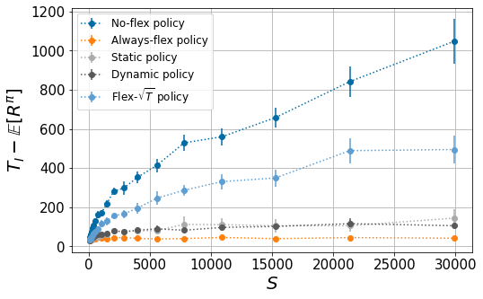
(a)

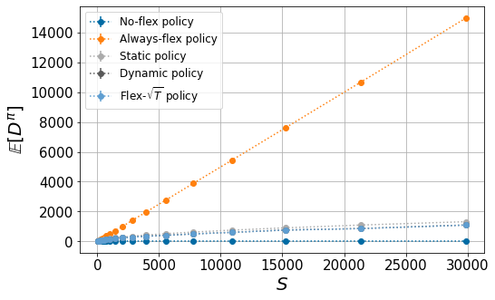
(b)

Figure 1: Performance under the no-flex, always-flex, static, dynamic and flex-$\sqrt{T}$ policies.

We next (Figure 2) compare the total costs of these policies under different regimes of $\delta,K$ and $h$ (see Appendix B.4 for theoretical bounds). In particular, we set $K=\frac{NS}{2}$ and $h=\frac{1}{NS}$ (values for which the EOQ formula, $NS=\sqrt{\frac{2K}{h}},$ is satisfied) and benchmark the performance of our policies against $\mathcal{C}^{\star}$, the theoretical lower bound on any policy’s total cost, under different regimes of $\delta$. In many of the regimes considered, all of the policies are asymptotically optimal with respect to $S$, i.e., the per-period loss relative to the lower-bound converges to $0$ as $S$ grows large. When $\delta=0$ (i.e., exerting flexibility incurs no cost, LABEL:fig:cost1a), the always-flex and no-flex policies are the best- and worst-performing policies, respectively. However, the dynamic and static policies’ performance is quite close to the always-flex policy, with the always-flex and dynamic policies seemingly converging at a linear rate. On the other extreme, when $\delta\in\Theta\left(\sqrt{S}\right)$ (i.e., discounts are very expensive, LABEL:fig:cost1d), the no-flex policy is the best-performing policy and the others cease to be asymptotically optimal. The most interesting cases arise when $\delta$ is constant (LABEL:fig:cost1c) or $\delta$ is slowly decreasing (i.e., $\delta\in\Theta\left(1/{\sqrt{S}}\right)$, LABEL:fig:cost1b): in the former case, the dynamic and static policies perform best (converging at rate $1/\sqrt{S}$ to the lower bound); the no-flex and the flex-$\sqrt{T}$ policies exhibit slightly worse performance but converge at the same rate to the lower bound, while the always-flex policy converges to a constant per-period loss. In the latter case, we again find that the dynamic policy converges at a linear rate and the static policy performs almost as well while in this case all of the benchmark policies converge much slower to the lower bound (seemingly at rate $1/\sqrt{S}$).

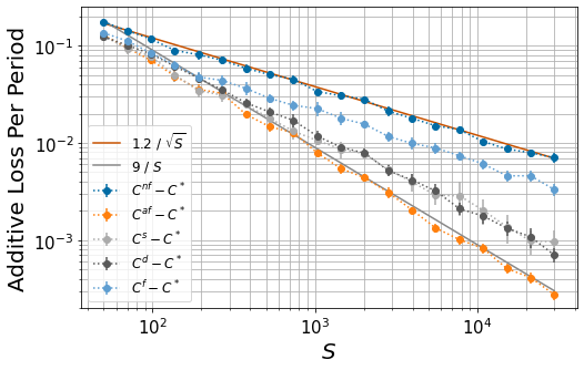
(a)

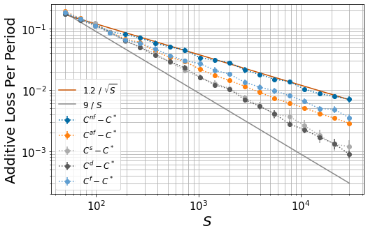
(b)

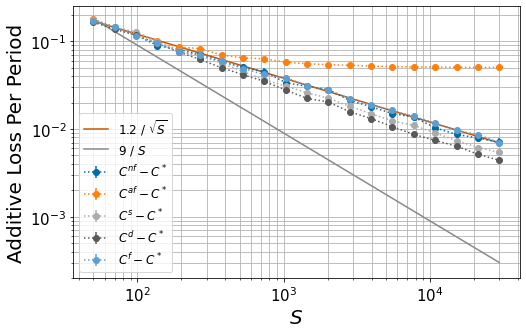
(c)

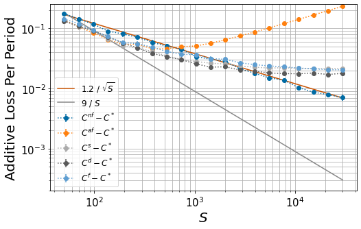
(d)

Figure 2: Additive loss of policy $\pi$ relative to $\mathcal{C}^{\star}$ under different regimes of $\delta$ (assuming $K=\frac{NS}{2},h=\frac{1}{NS}$) in the opaque selling model, for $\pi\in\{\pi^{nf},\pi^{a},\pi^{s},\pi^{d},\pi^{f}\}$.

Notably, LABEL:fig:cost1a to LABEL:fig:cost1c show that for any $\delta\in\mathcal{O}(1)$, $(i)$ the dynamic policy either performs better or as well as other policies, and $(ii)$ the static policy performs almost as well as the dynamic policy. LABEL:fig:cost1d explores a regime outside the scope of Theorem 4, allowing the opaque discount $\delta$ to scale with the initial inventory level $S.$ While this regime is unlikely to hold in practice, it illustrates that as $\delta$ increases, the no-flex policy begins to emerge as the best policy, while the always-flex policy has the worst performance. In summary, our three benchmark policies (always-flex, never-flex, and flex-$\sqrt{T}$) each demonstrate significant weaknesses in at least two out of the four settings. This then suggests that parsimoniously (yet strategically) exerting flexibility is a more robust strategy than the benchmarks that either aggressively manage the load of the system, don’t at all, or do so in a non-methodologically grounded way.

4 Data-Driven Case Study: Parcel Delivery

We next conduct a case study using data from the 2021 Amazon Last Mile Routing Research Challenge Dataset [MAP⁺22] to illustrate the applicability of our insights to parcel delivery in e-commerce fulfillment. This setting exhibits a similar challenge as the one at the crux of the basic balls-into-bins and opaque selling models. Namely, for a set of packages that arrive online over the course of a day, a retailer must efficiently assign packages to trucks. Practically speaking, this requires packages to be assigned in a way that maintains low travel times across all trucks, in addition to minimizing overtime compensation costs to delivery drivers (incurred when a route’s overall completion time exceeds a given threshold). An added complexity of this setting is that the completion times depend on both the number of packages assigned to a truck and their geographic location. Nonetheless, the online parcel delivery problem exhibits key features of our load balancing problem: the retailer seeks to balance final route completion times across trucks (i.e., after all packages have been assigned) as a way of avoiding overtime costs, but has to trade off this goal with the risk of inter-truck load balancing causing in hindsight costly detours.

Despite this conceptual similarity, the online routing aspect of the parcel delivery problem renders it significantly more complex than vanilla balls-into-bins. In particular, in the latter setting an individual flex reduces/increases the imbalance between two bins at the end of the horizon by at most one ball. In the former setting, however, characterizing the impact of moving a package from one truck to another is more involved, given its dependence on an a priori unknown final route (which also depends on the geographic location of future packages assigned to each truck). In this section we will see that “good” assignment policies need to account for these complexities. However, by appropriately incorporating these into our flexing condition we find that our policies for balls-into-bins directly extend, with strong empirical performance, to this more complicated setting.

4.1 Model

We consider a warehouse delivering packages in a region partitioned into $N$ different zones (e.g., a set of contiguous zip-codes), each served by one uncapacitated truck. A sequence of $T$ packages arrives and must be assigned (irrevocably) to one of $N$ trucks in an online fashion. (We address the uncapacitated assumption in Appendix C.6.) Each package $t$ is associated by default to a truck $P(t)$ corresponding to one of these zones. We provide further details as to how these zones are constructed in Section 4.2.

The goal is to minimize the total delivery costs of an assignment of packages to trucks, composed of: transportation (e.g., fuel) costs $c^{r}$ per hour; and overtime compensation of delivery drivers, i.e., a cost $c^{o}$ for every hour a driver works over an overtime threshold $h^{max}$ hours. Formally, let $y^{u}_{i}(t)$ and $y^{r}_{i}(t)$ respectively denote the unloading and travel times required by truck $i$ before the assignment of the $t$-th package, with the load of the truck denoted by $y_{i}(t)=y^{u}_{i}(t)+y^{r}_{i}(t)$.

$$\sum_{i}\mathbb{E}\left[c^{r}\cdot y^{r}_{i}(T+1)+c^{o}\cdot(y_{i}(T+1)-h^{max})^{+}\right],\qquad\text{{where $(\cdot)^{+}=\max\{\cdot,0\}$.}}$$ (3)

Analogy to balls-into-bins model.

Given (3), good policies should aim to $(i)$ minimize travel times, and $(ii)$ keep overall route completion times below the overtime threshold. Note that, since the zone assignment was determined using packages’ geographic coordinates, the default mapping should perform well in terms of the first objective. On the other hand, if demand for a particular zone comes in heavy on a given day, the associated route will incur a high unloading time and risk exceeding the overtime threshold $h^{max}$. Then, assigning packages from this cluster to different trucks may be beneficial. Doing so does not come for free, however, since adding a package to a truck may cause a detour, and hence additional transportation costs, as we will see in Section 4.3.

Table 1 compares the two models in order to draw the analogy that will drive our algorithm design. Given this analogy, we restrict our attention to the class of “flexibility-exerting” policies that sequentially determine $(i)$ when to assign an incoming package to a non-default truck, and $(ii)$ which truck to assign it to. For simplicity we assume that $q=1$, i.e., the decision to exert flexibility results in a flex being exerted; unless otherwise specified, the flex set $F(t)$ of an incoming package is the set of all zones such that the distance between package $t$ and the geographic center of the zone is within $1$ kilometer of the distance from $t$ to the center of the zone associated with $P(t)$.

	Balls-into-bins	Parcel delivery
Setup	$T$ balls; $N$ bins	$T$ packages; $N$ trucks
Load	Number of balls in bin	Unloading and travel times
Objective	Minimize $Gap(T)$	Minimize total delivery costs (3)

Table 1: Comparison of balls-into-bins and parcel delivery models

4.2 Dataset description

The 2021 Amazon Last Mile Routing Research Challenge Dataset [MAP⁺22] describes a set of historical routes used by Amazon drivers between July and August 2018, in the five metropolitan areas of Seattle, Los Angeles, Austin, Chicago, and Boston. We use the dataset that was previously created for training purposes in [MAP⁺22]. This dataset is composed of $6,112$ historical routes, and includes the following information about each route: its originating delivery station, the location of each stop on the route, and the time a delivery driver took to drop off each package (i.e., the unloading time, which [MAP⁺22] refer to as service time). Since all packages at the same stop have the same coordinates, for simplicity, we aggregate all packages associated with a stop into a single package whose unloading time is the sum of all component packages’ unloading times. Thus, we use the terms package and stop interchangeably.

Synthetic dataset construction.

We consider a single delivery station in Los Angeles, DLA8, over the course of 29 days, deferring results for two other stations in the dataset to Appendix C.5. In order to infer a default assignment of packages to trucks, we cluster all historical packages into $N=24$ routes based on their geographic coordinates (see Appendix C.2 for details on our clustering method). Fig. 3 provides an illustration of the output clustering, with each color representing a different zone. The number of trucks we use in our synthetic dataset is higher than the daily number of routes historically operated out of DLA8 ($N=15.4$, as seen in Table 2). This is due to the fact that our simulation samples from all package data over the 29-day period, which typically has a wider geographical span than that of any single day in the historical data and thus leads to a longer average travel time given the same number of packages per truck. (This may also be due in part to the pre-processing of the original dataset, in which geographic locations were perturbed to preserve driver and customer anonymity.) As a result, we increased the number of trucks to $N=24$ to ensure that the average route completion time under the no-flex policy matches the historical route completion time. We further compare the historical and synthetic datasets in Appendix C.3.

Finally, to simulate the stream of incoming packages over a given day, we bootstrapped from the sample distribution of all delivered packages over the recorded time period (see Table 2), taking $T=2,000$ to be the average number of daily packages. All reported results are averaged over 50 replications. We refer the reader to Table 3 for a summary of key inputs to our case study.

Number of routes per day				Number of stops per day				Number of packages per day
Mean	$Q_{1}$	Median	$Q_{3}$	Mean	$Q_{1}$	Median	$Q_{3}$	Mean	$Q_{1}$	Median	$Q_{3}$
$15.4$	$12.0$	$16.0$	$18.0$	$1977.9$	$1509.0$	$2066.0$	$2280.0$	$3833.9$	$2847.0$	$4020.0$	$4315.0$

Table 2: Historical Daily Statistics for DLA8

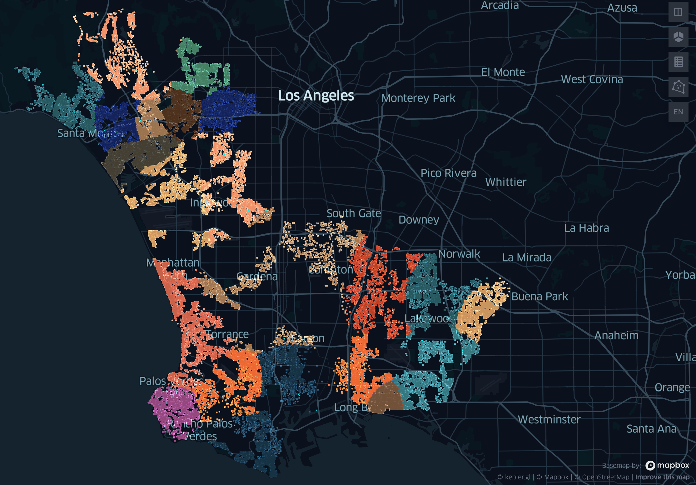
Figure 3: Clustering for Station DLA8

Input	Description	Value
$c^{r}$	Hourly transportation cost	$6.3
$c^{o}$	Hourly overtime cost	$38
$h^{max}$	Overtime threshold	$8$ hours
$N$	Number of trucks	$24$
$T$	Number of packages per day	$2,000$

Table 3: Summary of inputs. Derivations of cost terms can be found in Appendix C.1.

4.3 Results

On the importance of travel time considerations.

A first attempt that simplifies the complexities of the parcel delivery setting is to construct a routing-oblivious policy, which makes its flexing decision based solely on unloading times. Concretely, we apply the dynamic policy designed for the balls-into-bins problem (Algorithm 1) to this setting, letting $x^{d}_{i}(t)=y^{u}_{i}(t)\ \forall\ i\in[N],t\in[T]$, a flex radius of $5$ kilometers and an appropriately tuned $a_{d}$. When flexed, the package is assigned to the truck with the smallest current unloading time.

For our estimates of $c^{r}$ and $c^{o}$ (see Table 3), the routing-oblivious policy performs quite poorly, yielding a 126% increase in total costs on average (approximately $1,697 for the unloading-only policy, as opposed to $752.4 for the no-flex policy). Fig. 4 provides intuition for this poor performance: despite its effectiveness in balancing unloading times, the algorithm does so at a cost of significantly longer travel times (5.47 hours for the unloading-only policy versus 3.99 hours for the no-flex policy, on average). As a result, the unloading-only policy incurs much higher overtime: 80% of its routes are completed in over 8 hours with an average overtime of 0.95 hours, versus approximately 25% of no-flex routes completed in over 8 hours and an average overtime of 0.16 hours. Table 4 summarizes additional metrics of interest for the two policies.

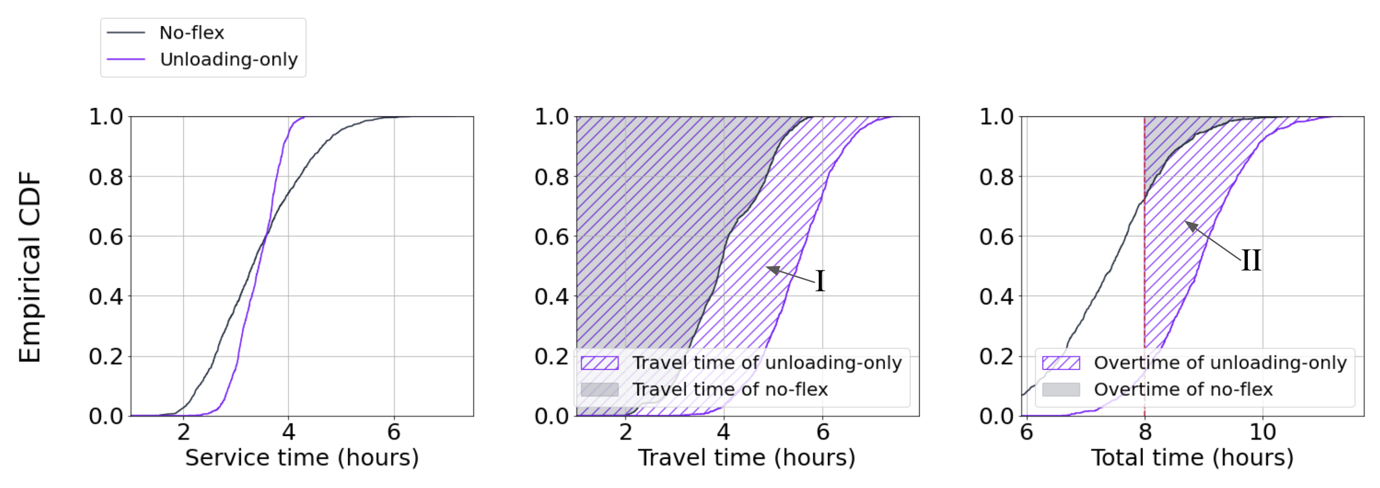
Figure 4: Distribution of unloading, travel, and total route completion times under the unloading-only and the no-flex policy across all simulation trails. Areas I and II respectively capture the additional travel time and overtime incurred by the unloading-only policy.

Policy	Unloading time			Travel time			Total time
	Mean	Abs. deviation	$Q_{3}-Q_{1}$	Mean	Abs. deviation	$Q_{3}-Q_{1}$	Mean	Overtime
No-flex	3.42	0.73	1.32	3.99	0.70	1.39	7.41	0.16
Unloading-only	3.42	0.34	0.63	5.47	0.64	1.10	8.89	0.95
Routing-Dynamic	3.42	0.80	1.47	4.33	0.47	0.79	7.75	0.21
Patient-Dynamic	3.42	0.73	1.35	4.12	0.59	1.09	7.53	0.10

Table 4: Route completion time statistics (in hours) for policies discussed in this section

A routing-aware dynamic policy.

The above results highlight the importance of considering both unloading and travel times in the parcel delivery setting. The natural extension of the routing-oblivious policy, then, would be to apply Algorithm 1 with $x^{d}_{i}(t)~{}=~{}y^{r}_{i}(t)+y^{u}_{i}(t)\ \forall\ i\in[N],t\in[T]$. We approximate $y^{r}_{i}(t)$ in each period as follows: for a set of packages $S$, denote by $\texttt{TSP}(S)$ the minimum travel time associated with a truck delivering these packages. Then, after every $100$ arrivals, for each truck $i$ we compute the optimal route $\texttt{TSP}(S_{i})$ for the packages currently assigned to $i$. In between updates, we approximate the incremental travel time associated with assigning package $t$ to truck $i$ as twice the distance from $t$ to the closest package currently assigned to $i$. We use $\texttt{INC}(S_{i},t)$ to denote this incremental travel time, given the current set of packages $S_{i}$. Letting $\tilde{y}_{i}^{r}(t)$ denote this approximate travel time, we apply Algorithm 1 with $x^{d}_{i}(t)~{}=~{}\tilde{y}_{i}^{r}(t)+y^{u}_{i}(t)$.

Experiments show that this application of Algorithm 1, which we refer to as the Routing-Dynamic policy, is also ineffective in reducing costs. The average cost of the no-flex policy is $\$752.4$, while that of the Routing-Dynamic policy is $\$850.4$, a $13\%$ increase. As shown in Table 4 and Fig. 5, while the Routing-Dynamic policy achieves lower travel times and overtime than the unloading-only policy, it performs worse on both fronts relative to the no-flex policy. Indeed, the average overtime of the Routing-Dynamic policy is $0.21$ hours versus an average overtime of $0.16$ hours for the no-flex policy; similarly, the travel time for the Routing-Dynamic policy averages $4.33$ hours of travel time as compared to $3.99$ hours for the no-flex policy.

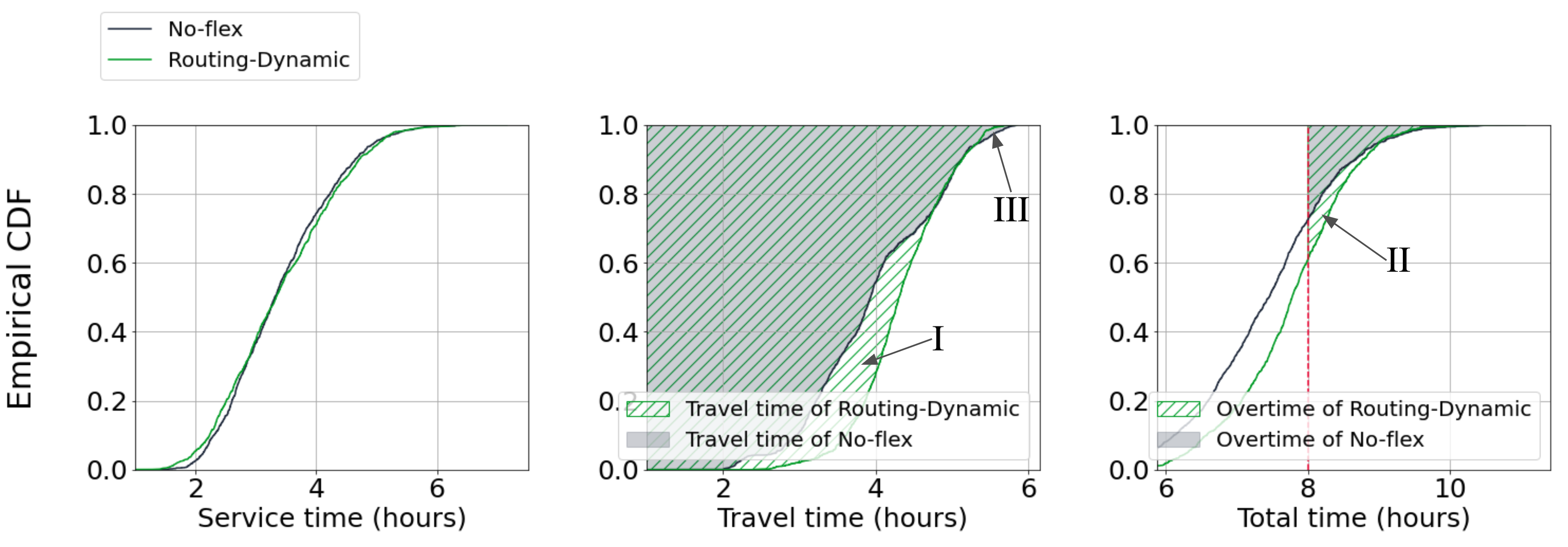
Figure 5: Distribution of unloading, travel, and total route completion times under the Routing-Dynamic and the no-flex policies. Areas I and II respectively capture the additional travel time and overtime required by the Routing-Dynamic policy. Area III captures the reduction in travel time of the Routing-Dynamic policy relative to the no-flex policy, which is negligible in this case.

At a high level, the Routing-Dynamic policy’s poor performance is due to the “looseness” of the flexing condition: in general, the largest load across all trucks may be much higher than the load of $P(t)$, for any given $t$. Thus, the Routing-Dynamic policy will flex frequently, causing costly detours when default trucks could have handled their respective packages in hindsight. This then highlights that, in the parcel delivery setting, policies must exert flexibility much more parsimoniously than in the balls-into-bins and inventory settings. Fig. 6 further illustrates why the current policy incurs high costs: the decision it makes in period $t$ is independent of the package $t$ at hand, an obviously bad decision in hindsight. The next policy we present addresses this shortcoming by incorporating the impact of package $t$ assignment on truck loads.

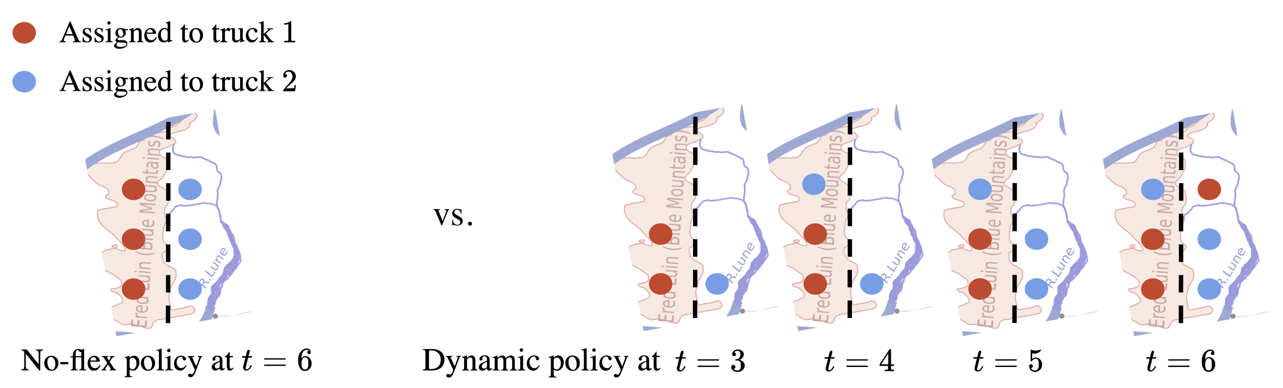
Figure 6: Stylized example illustrating the costliness of unnecessary flexing. Here we assume that the packages on the left-hand side of the map are by default assigned to Truck 1, and packages on the right-hand side of the map are by default assigned to Truck 2. At $t=4$, the Routing-Dynamic policy would assign the package on the left-hand side to Truck 2 to balance the unloading times of both trucks. At $t=5$, the incoming package side is assigned to its default truck to minimize the worst-case incremental travel distance. Finally, at $t=6$ the final package is assigned to Truck 1, to again balance unloading times. In hindsight, however, the no-flex policy would have been optimal.

Penalizing unnecessary flexing via a patient dynamic policy.

Our final policy — which we call the Patient-Dynamic policy — modifies the flexing condition to allow for flexing only when we estimate that the gap between the loads of the default truck $P(t)$ and some truck in the flex set $F(t)$ cannot be closed in the time remaining. To make this idea concrete, suppose first that our policy had access to the entire sequence of arrivals at the beginning of time. Then, in each period $t$ our policy would consider all possible packages that may be assigned to $P(t)$ (either because $P(t^{\prime})=P(t)$, or because $P(t)\in F(t^{\prime})$, for $t^{\prime}>t$). Let $\widehat{S}({t})$ denote this set of packages. Now, for truck $j\in F(t)$, we restrict our attention to the packages $t^{\prime}\in\widehat{S}({t})$ such that package $t^{\prime}$ is within the flexing radius of truck $j$. Let $\widehat{S}_{j}(t)$ denote this set of packages. Then, in the best case for truck $P(t)$, all packages in this set are placed in $j$, and the packages that a $(P(t),j)$ flex cannot control do not further contribute to the imbalance between the two. If, even in this best-case scenario, the load of $P(t)$ exceeds that of $j$, we consider $P(t)$ to be “over-loaded” and a flex is required. We then flex into $j\in F(t)$ with the minimum load.

The main challenge here is that our policy does not have offline access to all arriving packages. Hence, we must construct estimates of these future loads in every period. To construct these estimates, for every pair of trucks $i,j\in[N]$, we use $\texttt{INC}_{i,j}$ and $\texttt{SER}_{i,j}$ to respectively denote estimates of the average travel and unloading times added onto a no-flex route if a package whose default truck is $i$ is flexed into truck $j$. To compute $\texttt{INC}_{i,j}$, we simulate 50 replications of the no-flex policy over the entire time horizon. Under this policy, we consider the packages associated with truck $i$ that can be flexed into $j$, and compute the difference between the optimal TSP route with and without each of these packages. Averaging across all such packages, we obtain $\texttt{INC}_{i,j}$. The computation for $\texttt{SER}_{i,j}$ is analogous. Since $\texttt{INC}_{i,j}$ and $\texttt{SER}_{i,j}$ are averaged across all periods, we require an estimate of the average size of $\widehat{S}_{j}(t)$; we estimate this to be on the order of $(T-t)/M_{2}$, where $M_{2}$ is a tunable parameter. Finally, $\texttt{SER}(t)$ is used to denote the unloading time of package $t$. The Patient-Dynamic policy is described in Algorithm 2.

Algorithm 2 Patient-Dynamic Policy

1:Hyper-parameters $M_{1}=100$, $M_{2}=200$

2:$\tilde{y}_{i}^{r}(0)=0,y^{u}_{i}(0)=0,y_{i}(0)=0,v_{i}=\emptyset\;\forall\,i\in[N]$ 

3:for $t\in[T]$ do

4:     // Re-solve TSP every $M_{1}$ packages

5:     if $t\bmod M_{1}=0$ then

6:         $\tilde{y}_{i}^{r}(t)=\texttt{TSP}(v_{i}),y_{i}(t)=\tilde{y}_{i}^{r}(t)+y^{u}_{i}(t)\;\forall i$

7:     end if

8:     // Find the projected load of a flex truck when all future packages in this flex zone are assigned to it

9:     for $i\in F(t)$ do

10:         $\bar{y}_{i}=y_{i}(t)+\texttt{INC}(S_{i},t)+\texttt{SER}(t)+\frac{T-t}{M_{2}}\cdot\left(\texttt{INC}_{P(t),i}+\texttt{SER}_{P(t),i}\right)$

11:     end for

12:     // Flex package into projected ‘‘minimally-loaded’’ truck if load of default truck exceeds it

13:     if $y_{P(t)}(t)+\texttt{INC}(S_{P(t)},t)+\texttt{SER}(t)\geq\min_{i\in F(t)}\bar{y}_{i}$ then

14:         $\mathcal{A}(t)=\operatorname*{arg\,min}_{i\in F(t)}\bar{y}_{i}$

15:     else $\mathcal{A}(t)=P(t)$

16:     end if

17:     // Update truck loads

18:     $S_{\mathcal{A}(t)}\leftarrow S_{\mathcal{A}(t)}\cup\{l_{t}\}$

19:     $\tilde{y}_{i}^{r}(t+1)=\begin{cases}\tilde{y}_{i}^{r}(t)+\texttt{INC}(S_{\mathcal{A}(t)},t)\quad\text{if }i=\mathcal{A}(t)\\ \tilde{y}_{i}^{r}(t)\quad\text{otherwise}\end{cases}$,

20:     ${y}_{i}^{u}(t+1)=\begin{cases}{y}_{i}^{u}(t)+\texttt{SER}(t)\quad\text{if }i=\mathcal{A}(t)\\ {y}_{i}^{u}(t)\quad\text{otherwise}\end{cases}$

21:     $y_{i}(t+1)=\tilde{y}_{i}^{r}(t+1)+y_{i}^{u}(t+1)\,\forall\ i\in[N].$

22:end for

Remark 2.

Ignoring the routing aspects and the heterogeneity in unloading times, this intuition is consistent with that in Algorithm 1 for balls-into-bins. There, a ball is flexed into a minimally loaded bin when the imbalance between the maximally loaded bin and the average load exceeds $a_{{d}}$ times the average number of flexes remaining between the maximally and minimally loaded bins. Intuitively, Algorithm 2 redefines the gap as the difference between the loads of the default and the minimally loaded bins. The proofs of Theorems 2 and 3 extend to this modified benchmark.

We find that the Patient-Dynamic policy yields significant cost savings, with an overall cost reduction of 5.47% relative to the no-flex policy ($711.3 versus $752.4, on average). In Fig. 7 we observe that though the Patient-Dynamic policy incurs slightly higher travel times on average, its route completion times are more tightly concentrated around 8 hours. This then results in average overtime decreasing from 0.16 hours to 0.10 hours, from which our policy derives its gains.

We test the sensitivity of our results in Table 5, comparing the performance of the two policies as travel costs, overtime costs, and overtime thresholds respectively vary. When travel costs are low, and overtime costs high, our policy achieves more than 7% cost savings relative to the no-flex policy. The difference between the two, however, drops significantly as the overtime threshold increases: this is due to the fact that almost all routes are completed within 9 hours for both policies.

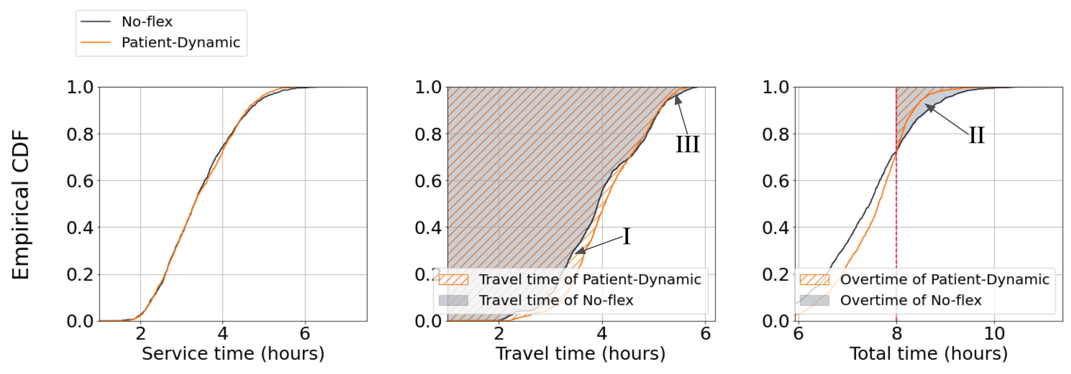
Figure 7: Distribution of unloading, travel, and total route completion times under the Patient-Dynamic and the no-flex policies. Area I captures the additional travel time required by the Patient-Dynamic policy. Areas II and III respectively capture the reduction in overtime and travel time of the Patient-Dynamic policy relative to the no-flex policy.

Parameters			Costs
Travel cost	Overtime cost	Overtime threshold	No-flex	Patient-Dynamic	Relative difference
5.00	38.00	8.00	627.99	582.85	-7.18%
5.50	38.00	8.00	675.84	632.26	-6.45%
6.00	38.00	8.00	723.71	681.66	-5.81%
6.50	38.00	8.00	771.59	731.07	-5.25%
7.00	38.00	8.00	819.46	780.48	-4.76%
7.50	38.00	8.00	867.34	829.88	-4.32%
6.30	32.00	8.00	728.88	697.29	-4.33%
6.30	34.00	8.00	736.73	701.96	-4.72%
6.30	36.00	8.00	744.58	706.63	-5.10%
6.30	38.00	8.00	752.44	711.31	-5.47%
6.30	40.00	8.00	760.29	715.98	-5.83%
6.30	42.00	8.00	768.15	720.65	-6.18%
6.30	38.00	7.50	921.07	909.88	-1.16%
6.30	38.00	8.00	752.44	711.31	-5.47%
6.30	38.00	8.50	664.44	643.30	-3.18%
6.30	38.00	9.00	625.17	628.74	0.57%
6.30	38.00	9.50	610.69	624.48	2.26%

Table 5: Sensitivity analyses for the costs of no-flex and Patient-Dynamic policies

We conclude the section by noting that the Patient-Dynamic policy yields cost savings relative to the no-flex policy, despite its decision rule being divorced from the actual travel and overtime costs. Another style of policy that one could consider is one that seeks to minimize the incremental cost of a flex, in each period. We explore this in Appendix C.4, and observe that doing so introduces additional levels of complexity (in particular, estimating the incremental cost of an action online) that prevent it from achieving the magnitude of cost savings achieved by our more simple, “informationally light” policy.

5 Conclusion

In this work we studied a variation of typical load balancing problems, in which the load needs to be balanced only at a specific, potentially random, point in time. We focused on three instantiations of this problem: the canonical balls-into-bins problem (used in computing applications), optimal opaque selling strategies (used in inventory management), and parcel delivery (used in e-commerce fulfillment). For these diverse applications we designed practical heuristics that sparingly exert flexibility and provably achieve approximate balance at the end of the horizon while achieving substantial cost savings.

This work opens several avenues for future exploration. Though our findings point to our heuristics’ broad applicability in load balancing applications where imbalance predominantly stems from stochastic fluctuations, it would be interesting to explore similar ideas in settings with first-order supply-demand imbalances. Secondly, blending our balancing strategies — which heavily focus on rebalancing near the end of the horizon — with existing policies in these domains could present new opportunities. This integration could lead to hybrid models that encapsulate the strengths of both traditional heuristics in these domains and our insights. For instance, for the parcel delivery problem it would be interesting to design provable algorithms that adapt state-of-the-art online VRP solutions to include balancing considerations. Lastly, tighter analyses could yield stronger guarantees in non-asymptotic regimes. These would be particularly beneficial in problems with short or fluctuating time horizons and may require new models to better capture these regimes.

Appendix A The Balls-Into-Bins Model

A.1 Analysis of the static policy

A.1.1 Algorithm

Before providing a formal description of the algorithm, we recall some notation. For $t\in[T]$, we let $x^{s}_{i}(t)$ denote the number of balls in bin $i\in[N]$ under the static policy, and use $\mathcal{A}^{s}(t)$ to denote the bin in which the ball lands at time $t$. Finally, we let $Gap^{s}(T)$ denote the gap of the system at time $T$ under the static policy. A formal description of the static policy is then provided in Algorithm 3 (with ties assumed to be broken lexicographically within the $\operatorname*{arg\,min}$.)

Algorithm 3 Static Policy $\pi^{s}$

1:$x^{s}_{i}(0)=0\;\forall\,i\in[N]$, $a_{{s}}=\frac{2\sqrt{6}N(N-1)}{q}$, $\omega(t)=\begin{cases}0\quad t<T-a_{{s}}\cdot\sqrt{T\log(T)}\\ 1\quad\text{otherwise}\end{cases}$ 

2:for $t\in[T]$ do

3:     if $\omega(t)f(t)=1$ then

4:         $\mathcal{A}^{s}(t)=\operatorname*{arg\,min}\limits_{i\in F(t)}x^{s}_{i}(t)$

5:     else

6:         $\mathcal{A}^{s}(t)=P(t)$

7:     end if

8:     for $i\in[N]$ do

9:         $x^{s}_{i}(t+1)=\begin{cases}x^{s}_{i}(t)+1&\quad\text{if }i=\mathcal{A}^{s}(t)\\ x^{s}_{i}(t)&\quad\text{otherwise}.\end{cases}$

10:     end for

11:end for

A.1.2 Proof of Proposition 1

Proof.

We first state Claim 1, with its proof deferred to the end of the section.

Claim 1.

For the never-flex policy $\pi^{nf}$, for any $a>0,$ there exists a constant $a^{\prime}>0$ such that

$$\mathbb{P}\left(Gap^{nf}(T)\geq a\sqrt{T}\right)\geq a^{\prime}$$

for large enough $T$.

Plugging $a=2$ into Claim 1, there exists $a^{\prime}>0$ such that $\mathbb{P}\left(Gap^{nf}(T)\geq 2\sqrt{T}\right)\geq a^{\prime}$ for large enough $T.$ Now, consider a particular history $\sigma(T)\in\Sigma(T)$ with $Gap^{nf}(T)\geq 2\sqrt{T},$ and pick $i=\operatorname*{arg\,max}_{i^{\prime}}x_{i^{\prime}}(T)$. By definition, $Gap^{nf}(T)\geq 2\sqrt{T}$ implies $\sum_{t=1}^{T}\mathbbm{1}_{P(t)=i}\geq T/N+2\sqrt{T}.$ Suppose now that $\pi$ has full information on the realization of the $T$ random trials, and can arbitrarily set $\mathcal{A}^{\pi}(t)=j$, where $j\neq i,$ whenever $P(t)=i.$ That is, each time $\pi$ sets $\omega(t)=1$ it replaces one of the at least $T/N+2\sqrt{T}$ balls that go into bin $i$ with a flex ball that goes into some other bin and decreases $Gap^{\pi}(T)$ by $1$. It then follows that, if $M^{\pi}\leq\sqrt{T}$:

$$\mathbb{E}\left[Gap^{\pi}(T)\right] \geq\mathbb{E}\left[Gap^{\pi}(T)\mid Gap^{nf}(T)\geq 2\sqrt{T}\right]\cdot\mathbb{P}\left(Gap^{nf}(T)\geq 2\sqrt{T}\right)$$

$$\geq\mathbb{E}\left[Gap^{nf}(T)-\sqrt{T}\mid Gap^{nf}(T)\geq 2\sqrt{T}\right]\cdot a\geq\sqrt{T}\cdot a$$

for large enough $T$, which contradicts the fact that $\mathbb{E}\left[Gap^{\pi}(T)\right]\in\mathcal{O}(1)$.

Thus,

$$\mathbb{E}[M^{\pi}]\geq\mathbb{E}\left[M^{\pi}\mid Gap^{nf}(T)\geq 2\sqrt{T}\right]\cdot\mathbb{P}\left(Gap^{nf}(T)\geq 2\sqrt{T}\right)\geq\sqrt{T}\cdot a$$

for large enough $T$.∎

Proof of Claim 1..

We have:

$$\mathbb{P}(Gap^{nf}(T)\geq a\sqrt{T}) =\mathbb{P}\left(\max_{i^{\prime}}x_{i^{\prime}}(T)-\frac{T}{N}\geq a\sqrt{T}\right)\geq\mathbb{P}\left(x_{1}(T)-\frac{T}{N}\geq a\sqrt{T}\right)$$

$$=\mathbb{P}\left(\frac{x_{1}(T)-\frac{T}{N}}{\sqrt{T}\sigma}\geq\frac{a}{\sigma}\right),$$

where $\sigma=\frac{1}{N}(1-\frac{1}{N}).$ By the Berry-Esseen Theorem ([Fel], Chapter XVI.5, Theorem 2):

$$\mathbb{P}\left(\frac{x_{1}(T)-\frac{T}{N}}{\sqrt{T}\sigma}\geq\frac{a}{\sigma}\right)\geq 1-\Phi\left(\frac{a}{\sigma}\right)-\frac{b}{\sqrt{T}}\geq a^{\prime},$$

for some constants $a^{\prime}$, $b$ and large enough $T$. ∎

A.1.3 Lower bound for deterministic policies

Proposition 2.

For a policy $\pi$, at most one of the two holds:

1. $M^{\pi}\leq a\sqrt{T}$ almost surely, for some $a>0$, or

2. $\mathbb{E}\left[Gap^{\pi}(T)\right]\in o\left(\sqrt{T}\right).$

Proof.

We prove the claim by contradiction. Suppose there exists a policy $\pi$ such that $M^{\pi}\leq a\sqrt{T}$ for some constant $a>0$ and $\mathbb{E}[Gap^{\pi}(T)]\in o(\sqrt{T}).$

When no flexing is involved, by Claim 1, $\mathbb{P}\left(Gap^{nf}(T)\geq(a+1)\sqrt{T}\right)\geq a^{\prime},$ for some constant $a^{\prime}>0$ and large enough $T.$

Now, consider a particular history $\sigma(T)\in\Sigma(T)$ such that $Gap^{nf}(T)\geq(a+1)\sqrt{T},$ and consider $i\in\operatorname*{arg\,max}_{i^{\prime}}x_{i^{\prime}}(T)$. By definition, $Gap^{nf}(T)\geq(a+1)\sqrt{T}$ implies $\sum_{t=1}^{T}\mathbbm{1}_{P(t)=i}\geq T/N+(a+1)\sqrt{T}.$ Suppose now that $\pi$ knows the exact realization of the $T$ random balls, i.e., knows $\sigma(T)$, and, for all $t$ such that $P(t)=i$ and $\omega(t)=1$, can place the ball that would have gone into bin $i$ into any bin $j$ that decreased $Gap^{\pi}(T)$ by 1. Then, if $M^{\pi}\leq a\sqrt{T}$, $\pi$ can relocate at most $a\sqrt{T}$ balls from bin $i$ to the other bins and thus

$$\mathbb{E}\left[Gap^{\pi}(T)\right] \geq\mathbb{E}\left[Gap^{\pi}(T)\mid Gap^{nf}(T)\geq(a+1)\sqrt{T}\right]\cdot\mathbb{P}\left(Gap^{nf}(T)\geq(a+1)\sqrt{T}\right)$$

$$\geq\mathbb{E}\left[Gap^{nf}(T)-a\sqrt{T}\mid Gap^{nf}(T)\geq(a+1)\sqrt{T}\right]\cdot a^{\prime}$$

$$\geq\sqrt{T}\cdot a^{\prime}$$

for large enough $T$, which contradicts the fact that $\mathbb{E}[Gap^{\pi}(T)]\in o\left(\sqrt{T}\right)$. ∎

A.1.4 Proof of Theorem 1

Before proving the theorem, we present a result from the literature to characterize the gap at time $t$ under the always-flex policy.

Lemma 1 (Corollary 2.3 in [PTW10]).

$\mathbb{E}[Gap^{a}(t)]\in\Theta(1)\quad\forall\ t\in[T].$

We next define a class of fictional allocation rules that we couple to any flexing policy $\pi$.

Definition 1.

We define the allocation rule $\mathcal{A}_{ij}(t)$ as

$$\mathcal{A}_{ij}(t):=\begin{cases}j\quad&\text{if }f(t)\omega(t)=1\text{ and }F(t)=\{i,j\},\\ j\quad&\text{if }f(t)\omega(t)=1,F(t)=\{k,j\}\text{ for some }k\neq i\text{ and }\arg\min_{j^{\prime}\in\{i,k\}}x^{\pi}_{j^{\prime}}(t)=i,\\ \mathcal{A}^{\pi}(t)&\text{otherwise}.\end{cases}$$

The allocation rule $\mathcal{A}_{ij}$ mimics $\mathcal{A}^{\pi}$, except in two scenarios: when choosing between $i$ and $j$, $\mathcal{A}_{ij}$ always places a ball into $j$; and when choosing between $j$ and $k\neq i$, $\mathcal{A}_{ij}$ places a ball into $j$ if the policy $\pi$ would place a ball into $i$ rather than $k$ in period $t$ (with respect to its own load). At a high level, $\mathcal{A}_{ij}$ favors bin $j$ over bin $i$. We have the following lemma.

Lemma 2.

Suppose $\bar{t}$ balls are thrown into $N$ bins according to $\mathcal{A}_{ij}$, with each ball being a flex ball with probability $q$. Moreover, let $Y_{k}(\bar{t}),k\in[N]$, denote the number of flex balls, among the $\bar{t}$ throws, that are placed into bin $k$. Then, there exists some constant $\alpha>0$ such that

1. $\mathbb{E}[Y_{j}(\bar{t})-Y_{i}(\bar{t})]\geq\frac{q}{\binom{N}{2}}\bar{t}$,

2. $\mathbb{P}\left(Y_{j}(\bar{t})-Y_{i}(\bar{t})\leq\frac{q}{2\binom{N}{2}}\bar{t}\right)\leq e^{-\alpha\bar{t}}$.

The next lemma presents Binomial tail bounds that we use throughout our analysis.

Lemma 3.

Consider two binomial random variables $X_{i}(t)\sim B(t,p_{i}),X_{j}(t)\sim B(t,p_{j})$, where $X_{i}(t)$ and $X_{j}(t)$ need not be independent. Then, for any $\epsilon>0$:

1. $\mathbb{P}\left(\left|(X_{j}(t)-X_{i}(t))-\mathbb{E}[X_{j}(t)-X_{i}(t)]\right|\geq\epsilon t\right)\leq 4e^{-\epsilon^{2}t/2}$,

2. $\mathbb{P}\left(\left|(X_{j}(t)-X_{i}(t))-\mathbb{E}[X_{j}(t)-X_{i}(t)]\right|\geq\epsilon\sqrt{t\log(t)}\right)\leq 4t^{-\epsilon^{2}/2}.$

We leverage Lemma 2 and Lemma 3 to prove Theorem 1 next, and defer their proofs to Appendix A.1.5.

Proof of Theorem 1..

Let $\widehat{T}=T-a_{{s}}\cdot\sqrt{T\log(T)}$. By construction, the static policy starts flexing at $\widehat{T}+1$. Let $E$ denote the event that the gap is non-zero at $T$. Then,

$$\mathbb{E}[Gap^{s}(T)]=\mathbb{E}[Gap^{s}(T)\mid E]\mathbb{P}(E)+\mathbb{E}[Gap^{s}(T)\mid E^{c}]\mathbb{P}(E^{c})=\mathbb{E}[Gap^{s}(T)\mid E]\mathbb{P}(E),$$ (4)

where the second equality follows from the fact that $Gap^{s}(T)=0$ given $E^{c}$, by definition.

Let $E^{1}$ denote the event that the maximally and minimally loaded bins at time $T$ never have the same loads between $\widehat{T}$ and $T$, and $E^{2}$ the event that they do. Letting $\tau$ denote the last period in which the loads of the maximally and minimally loaded bins at time $T$ were equal, we have:

$$\mathbb{E}[Gap^{s}(T)] =\mathbb{E}\left[Gap^{s}(T)\mid E^{1}\right]\mathbb{P}\left(E^{1}\right)+\mathbb{E}\left[Gap^{s}(T)\mid E^{2}\right]\mathbb{P}\left(E^{2}\right)$$ (5)

$$\leq T\mathbb{P}\left(E^{1}\right)+\mathbb{E}\left[T-\tau\mid E^{2}\right]\mathbb{P}\left(E^{2}\right),$$ (6)

where the inequality follows from the fact that under $E^{2}$, in the worst case, all balls between $\tau$ and $T$ land in the maximally loaded bin, resulting in $Gap^{s}(T)\leq T-\tau$.

For $i,j\in[N]$, we use $E_{ij}^{1}$ to denote the event that (a) $i$ and $j$ are respectively the maximally and minimally loaded bins at time $T$, and (b) the loads of $i$ and $j$ are never the same between $\widehat{T}$ and $T$. We moreover use $E_{ij}^{2}$ to denote the event that (a) $i$ and $j$ are respectively the maximally and minimally loaded bins at time $T$ and do not have the same loads, but (b) their loads were the same at some point between $\widehat{T}$ and $T-1$. Formally:

$$E_{ij}^{1}:=\{ \sigma(T)\in\Sigma(T)\mid i=\arg\max_{k\in[N]}x^{s}_{k}(T),j=\arg\min_{k\in[N]}x^{s}_{k}(T),x^{s}_{i}(t)\neq x^{s}_{j}(t),\forall t\in\{\widehat{T},\ldots,T\}\}$$ (7)

$$E_{ij}^{2}:=\{ \sigma(T)\in\Sigma(T)\mid i=\arg\max_{k\in[N]}x^{s}_{k}(T),j=\arg\min_{k\in[N]}x^{s}_{k}(T),$$

$$\hskip 71.13188ptx^{s}_{i}(t)=x^{s}_{j}(t)\text{ for some }t\in\{\widehat{T},\ldots,T-1\},x^{s}_{i}(T)\neq x^{s}_{j}(T)\}$$ (8)

Since $E\subseteq\cup_{i\neq j}E_{ij}^{1}\cup E_{ij}^{2}$, we further bound (5) as follows:

$$\mathbb{E}\left[Gap^{s}(T)\right] \leq T\sum_{i\neq j}\mathbb{P}\left(E_{ij}^{1}\right)+\sum_{t=1}^{T-\widehat{T}}\sum_{i\neq j}t\mathbb{P}\left(E_{ij}^{2},T-\tau=t\right)$$ (9)

$$\leq T\sum_{i\neq j}\mathbb{P}\left(E_{ij}^{1}\right)+\sum_{t=1}^{T-\widehat{T}}\sum_{i\neq j}t\mathbb{P}\left(E_{ij}^{2}\mid T-\tau=t\right).$$ (10)

We decompose the remainder of the proof into two steps. In Step 1, we first show that there exist constants $\beta_{1}>0,\alpha_{1}>0$ such that for large enough $T$

$$\mathbb{P}(E_{ij}^{1})\leq\beta_{1}T^{-2}+e^{-\alpha_{1}(T-\widehat{T})}\qquad\forall\ i,j.$$ (11)

In Step 2 we argue that there exist constants $\alpha_{2}>0,\alpha_{3}>0$ such that

$$\mathbb{P}\left(E_{ij}^{2}|T-\tau=t\right)\leq 4e^{-\alpha_{2}t}+e^{-\alpha_{3}t}\quad\forall\ i,j.$$ (12)

Plugging (11) and (12) back into (9), we then obtain that, for large enough $T$,

$$\mathbb{E}\left[Gap^{s}(T)\right]\leq \sum_{i\neq j}T(\beta_{1}T^{-2}+e^{-\alpha_{1}(T-\widehat{T})})+\sum_{i\neq j}\sum_{t=1}^{T-\widehat{T}}t(4e^{-\alpha_{2}t}+e^{-\alpha_{3}t})\in\mathcal{O}(1),$$

which completes the proof of the theorem.

Step 1: Bound $\mathbb{P}(E_{ij}^{1})$, for all $i,j\in[N]$.

We state the following lemma, and defer its proof to Appendix A.1.5.

Lemma 4.

Consider any policy $\pi$ that (a) sets $\omega(t)=0$ for $t\leq t_{1}$ (b) sets $\omega(t)=1$ for $t_{1}<t\leq t_{2}$, where $t_{2}-t_{1}\geq a_{{s}}\sqrt{t_{2}\log t_{2}}.$ Define

$$F_{ij}^{1}=\{\sigma(t_{2})\in\Sigma(t_{2})\mid i=\arg\max_{k\in[N]}x^{\mathcal{\pi}}_{k}(t_{2}),j=\arg\min_{k\in[N]}x^{\mathcal{\pi}}_{k}(t_{2}),x^{\mathcal{\pi}}_{i}(t)\neq x^{\mathcal{\pi}}_{j}(t),\forall t\in\{t_{1},\ldots,t_{2}\}\}.$$

Then, $\mathbb{P}(F_{ij}^{1})\leq\beta{t}_{1}^{-2}+e^{-\alpha_{1}(t_{2}-t_{1})}\ \forall\ i,j$ for some constants $\beta>0$, $\alpha_{1}>0$.

Applying Lemma 4 to event $E_{ij}^{1}$, with $t_{1}=\widehat{T}$ and $t_{2}=T$, for all $i,j\in[N]$ we have that $\mathbb{P}(E_{ij}^{1})\leq\beta\widehat{T}^{-2}+e^{-\alpha_{1}(T-\widehat{T})}.$ Using the fact that $\widehat{T}=T-a_{{s}}\sqrt{T\log(T)}$ we obtain Step 1.

Step 2: Bound $\mathbb{P}\left(E_{ij}^{2}|T-\tau=t\right)$ for all $i,j\in[N]$, $t\in\{1,\ldots,T-\widehat{T}\}$.

Again, we establish a general lemma for the probability bound and defer its proof to Appendix A.1.5.

Lemma 5.

Consider any policy $\pi$ that sets $\omega(t)=1$ for $t_{1}<t\leq t_{2}$. Define

$$F_{ij}^{2}:=\{ \sigma(t_{2})\in\Sigma(t_{2})\mid i=\arg\max_{k\in[N]}x^{\mathcal{\pi}}_{k}(t_{2}),j=\arg\min_{k\in[N]}x^{\mathcal{\pi}}_{k}(t_{2}),$$

$$\hskip 71.13188ptx^{\mathcal{\pi}}_{i}(t)=x^{\mathcal{\pi}}_{j}(t)\text{ for some }t\in\{t_{1},\ldots,t_{2}-1\},x^{\mathcal{\pi}}_{i}(t_{2})\neq x^{\mathcal{\pi}}_{j}(t_{2})\}.$$

Then, for $\tau:=\max\left\{t\,\mid\,x^{\mathcal{\pi}}_{i}(t)=x^{\mathcal{\pi}}_{j}(t),t\in\{t_{1},\ldots,t_{2}-1\}\right\}$, we have $\mathbb{P}(F_{ij}^{2}|t_{2}-\tau=t)\leq 4e^{-\alpha_{2}t}+e^{-\alpha_{3}t},\forall i,j$ for some constants $\alpha_{2}>0,\alpha_{3}>0$.

Applying Lemma 5 to $E_{ij}^{2}$, with $t_{1}=\widehat{T}$ and $t_{2}=T,$ we have that $\mathbb{P}(E_{ij}^{2}\mid T-\tau=t)\leq 4e^{-\alpha_{2}t}+e^{-\alpha_{3}t}\ \forall\ i,j$ for some $\alpha_{2},\alpha_{3}>0$, which completes the proof. ∎

A.1.5 Proofs of Auxiliary Results

Proof of Lemma 2..

Let $M=\sum_{t=1}^{\bar{t}}\mathbbm{1}_{F(t)=\{i,j\}}$. We have:

$$\mathbb{E}[Y_{j}(\bar{t})-Y_{i}(\bar{t})\mid M] =\mathbb{E}[Y_{j}(\bar{t})\mid M]-\mathbb{E}[Y_{i}(\bar{t})\mid M]$$

$$=M+\sum_{t=1}^{\bar{t}}\mathbb{P}\left(\{F(t)=\{j,k\}\text{ for some }k\neq i\}\cap\{\mathcal{A}_{ij}(t)=j\}\mid M\right)$$

$$\qquad-\sum_{t=1}^{\bar{t}}\mathbb{P}\left(\{F(t)=\{i,k\}\text{ for some }k\neq j\}\cap\{\mathcal{A}_{ij}(t)=i\}\mid M\right),$$

where the second equality follows from the fact that, by construction, whenever $F(t)=\{i,j\}$ (this happens $M$ times, by definition), the ball was allocated to bin $j$. By symmetry, $i$ and $j$ are equally likely to be included in $F(t)$. Combining this with the $\mathcal{A}_{ij}$ construction, which places a ball into bin $j$ whenever the static policy would have placed it into $i$ rather than $k$, we have:

$$\mathbb{E}[Y_{j}(\bar{t})-Y_{i}(\bar{t})\mid M]\geq M\implies\mathbb{E}[Y_{j}(\bar{t})-Y_{i}(\bar{t})]=\mathbb{E}[\mathbb{E}[Y_{j}(\bar{t})-Y_{i}(\bar{t})|M]]\geq\mathbb{E}[M]=\frac{q}{\binom{N}{2}}\bar{t}$$

and we obtain Lemma 2 (i).

We now prove Lemma 2 (ii). Let $W_{kt}$ be the random indicator variable representing whether a ball in period $t$ is a flex ball that goes into bin $k$, for $k\in[N],t\in[\bar{t}]$. Then, by definition, $Y_{k}(\bar{t})=\sum_{t=1}^{\bar{t}}W_{kt}\ \forall\ k\in[N]$. Define moreover $Z_{\tau}=\sum_{t=1}^{\tau}(W_{jt}-W_{it})-\frac{q}{\binom{N}{2}}\tau$ for $\tau=1,2,...,\bar{t}$, with $Z_{0}=0$. Then,

$$\mathbb{P}\left(Y_{j}(\bar{t})-Y_{i}(\bar{t})\leq\frac{q}{2\binom{N}{2}}\bar{t}\right) =\mathbb{P}\left(\sum_{t=1}^{\bar{t}}(W_{jt}-W_{it})\leq\frac{q}{2\binom{N}{2}}\bar{t}\right)=\mathbb{P}\left(Z_{\bar{t}}-Z_{0}\leq-\frac{q}{2\binom{N}{2}}\bar{t}\right).$$ (13)

We argue that the sequence $Z_{0},Z_{1},Z_{2}...$ is a sub-martingale:

$$\mathbb{E}[Z_{\tau+1}|Z_{0},...,Z_{\tau}] =\mathbb{E}\left[\sum_{t=0}^{\tau+1}W_{jt}-W_{it}-\frac{q}{\binom{N}{2}}(\tau+1)\;\bigg{|}\;Z_{0},...,Z_{\tau}\right]$$ (14)

$$=\mathbb{E}\left[W_{j,\tau+1}-W_{i,\tau+1}-\frac{q}{\binom{N}{2}}+Z_{\tau}\;\bigg{|}\;Z_{0},...,Z_{\tau}\right]$$

$$=\mathbb{E}\left[W_{j,\tau+1}-W_{i,\tau+1}\;\bigg{|}\;Z_{0},...,Z_{\tau}\right]-\frac{q}{\binom{N}{2}}+Z_{\tau}.$$ (15)

Note that a flex ball lands in bin $j$, i.e., $W_{jt}-W_{it}=1,$ if one of two events occurs: (1) $F(t)=\{i,j\}$, in which case the ball is always thrown into bin $j$, or (2) $F(t)=\{j,k\}$ for some $k\neq i,j$, and the ball is thrown into bin $j$. The first event occurs with probability $\frac{q}{\binom{N}{2}}$, and the second with probability $\mathbb{P}\left(\{F(t)=\{j,k\}\text{ for some }k\neq i\}\cap\{\mathcal{A}_{ij}(t)=j\}\right).$ Thus,

$$\mathbb{P}\left(W_{jt}-W_{it}=1\right)=\frac{q}{\binom{N}{2}}+\mathbb{P}\left(\{F(t)=\{j,k\}\text{ for some }k\neq i\}\cap\{\mathcal{A}_{ij}(t)=j\}\right).$$

Via similar reasoning, it follows that

$$\mathbb{P}\left(W_{jt}-W_{it}=-1\right)=\mathbb{P}\left(\{F(t)=\{i,k\}\text{ for some }k\neq j\}\cap\{\mathcal{A}_{ij}(t)=i\}\right).$$

Plugging this into (14):

$$\mathbb{E}[Z_{\tau+1}|Z_{0},...,Z_{\tau}] =\frac{q}{\binom{N}{2}}+\mathbb{P}\left(\{F(\tau+1)=\{j,k\}\text{ for some }k\neq i\}\cap\{\mathcal{A}_{ij}(\tau+1)=j\}\;\bigg{|}\;Z_{0},...,Z_{\tau}\right)$$

$$-\mathbb{P}\left(\{F(\tau+1)=\{i,k\}\text{ for some }k\neq j\}\cap\{\mathcal{A}_{ij}(\tau+1)=i\}\;\bigg{|}\;Z_{0},...,Z_{\tau}\right)$$

$$-\frac{q}{\binom{N}{2}}+Z_{\tau}$$

$$\geq Z_{\tau},$$ (16)

where the final inequality follows from the same arguments as those used to derive Lemma 2 (i) above. Having established $(Z_{\tau})_{t\in[T]}$ is a submartingale, we apply Azuma’s inequality [CL06] to (13), and obtain:

$$\mathbb{P}\left(Y_{j}(\bar{t})-Y_{i}(\bar{t})\leq\frac{q}{2\binom{N}{2}}\bar{t}\right)\leq e^{-\frac{2\cdot\left(\frac{q}{2\binom{N}{2}}\bar{t}\right)^{2}}{\bar{t}}}\leq e^{-\alpha\bar{t}}$$

for some constant $\alpha>0$.

∎

Proof of Lemma 3..

We first prove (i). We have:

$$\mathbb{P}\left(\left|(X_{j}(t)-X_{i}(t))-\mathbb{E}[X_{j}(t)-X_{i}(t)]\right|\geq\epsilon t\right) \leq\mathbb{P}\left(\left|(X_{j}(t)-\mathbb{E}\left[X_{j}(t)\right]\right|+\left|X_{i}(t)-\mathbb{E}\left[X_{i}(t)\right]\right|\geq\epsilon t\right)$$

$$\leq\mathbb{P}\left(\left|X_{j}(t)-\mathbb{E}[X_{j}(t)]\right|\geq\frac{\epsilon}{2}t\right)$$

$$\quad+\mathbb{P}\left(\left|X_{i}(t)-\mathbb{E}[X_{i}(t)]\right|\geq\frac{\epsilon}{2}t\right).$$ (17)

By Hoeffding’s inequality [DP09], for all $k\in[N]$,

$$\mathbb{P}\left(\left|X_{k}(t)-\mathbb{E}[X_{k}(t)]\right|\geq\frac{\epsilon}{2}t\right)\leq 2\exp\left(-\frac{\epsilon^{2}t}{2}\right).$$

Plugging this back into (A.1.5), we obtain:

$$\mathbb{P}\left(\left|(X_{j}(t)-X_{i}(t))-\mathbb{E}[X_{j}(t)-X_{i}(t)]\right|\geq\epsilon t\right)\leq 4e^{-\epsilon^{2}t/2}.$$

For (ii), we similarly have that

$$\mathbb{P}\left(\left|(X_{j}(t)-X_{i}(t))-\mathbb{E}[X_{j}(t)-X_{i}(t)]\right|\geq\epsilon\sqrt{t\log(t)}\right)$$

$$\leq\mathbb{P}\left(\left|X_{j}(t)-\mathbb{E}[X_{j}(t)]\right|\geq\frac{\epsilon}{2}\sqrt{t\log(t)}\right)+\mathbb{P}\left(\left|X_{i}(t)-\mathbb{E}[X_{i}(t)]\right|\geq\frac{\epsilon}{2}\sqrt{t\log(t)}\right).$$ (18)

As before, by Hoeffding’s inequality, for all $k\in[N]$,

$$\mathbb{P}\left(\left|X_{k}(t)-\mathbb{E}[X_{k}(t)]\right|\geq\frac{\epsilon}{2}\sqrt{t\log(t)}\right) \leq 2\exp\left(-\frac{\epsilon^{2}t\log t}{2t}\right)=2t^{-\epsilon^{2}/2}.$$

We thus obtain:

$$\mathbb{P}\left(\left|(X_{j}(t)-X_{i}(t))-\mathbb{E}[X_{j}(t)-X_{i}(t)]\right|\geq\epsilon\sqrt{t\log(t)}\right)\leq 4t^{-\epsilon^{2}/2}.$$

∎

Proof of Lemma 4..

We prove the claim via the coupling between $\mathcal{A}^{\pi}$ and $\mathcal{A}_{ij}$. We first introduce some additional notation. For bin $k\in[N]$, let $x_{k}^{\prime}(t)$ denote the load in bin $k$ and time $t$ under the fictional allocation policy $\mathcal{A}_{ij}$ (see Definition 1). We let $Y_{k}$ denote the number of flex balls that land in bin $k$ between $t_{1}+1$ and $t_{2}$ under $\mathcal{A}_{ij}$, and define $Y:=\sum_{k=1}^{N}Y_{k}$. Note that $Y\sim B\left(t_{2}-t_{1},q\right)$. We use $\overline{T}=t_{2}-Y$ to denote the total number of random (non-flex) throws throughout the entire time horizon, and use $Z_{k}$ to denote the number of balls that landed in bin $k$ during the $\overline{T}$ random trials. Thus, for $k\in[N]$, $x^{\prime}_{k}(t_{2})=Y_{k}+Z_{k}.$

Conditioned on the event $x^{\mathcal{\pi}}_{i}(t)>x^{\mathcal{\pi}}_{j}(t)\ \forall\ t\in\{t_{1},...,t_{2}\}$, $\mathcal{A}_{ij}$ and $\mathcal{A}^{\pi}$ make identical decisions, and as a result $x^{\prime}_{k}(t)=x^{\mathcal{\pi}}_{k}(t)\ \forall\ t\in\{t_{1},...,t_{2}\}$. Thus, we have:

$$F_{ij}^{1} :=\Bigg{\{}\sigma(t_{2})\in\Sigma(t_{2})\mid x^{\mathcal{\pi}}_{i}(t_{2})=\max_{k}x^{\mathcal{\pi}}_{k}(t_{2}),\,x^{\mathcal{\pi}}_{j}(t_{2})=\min_{k}x^{\mathcal{\pi}}_{k}(t_{2}),\,x^{\mathcal{\pi}}_{i}(t)>x^{\mathcal{\pi}}_{j}(t)\forall t\in\{t_{1},...,t_{2}\},$$

$$\hskip 76.82234ptx_{i}^{\prime}(t)>x_{j}^{\prime}(t)\,\forall\,t\in\{t_{1},...,t_{2}\}\Bigg{\}}$$

$$\subseteq\left\{\sigma(t_{2})\in\Sigma(t_{2})\mid x_{i}^{\prime}(t)>x_{j}^{\prime}(t)\,\forall\,t\in\{t_{1},...,t_{2}\}\right\}$$

$$\subseteq\left\{Y_{i}+Z_{i}>Y_{j}+Z_{j}\right\}.$$ (19)

We use (A.1.5) to bound $\mathbb{P}\left(F_{ij}^{1}\right)$:

$$\mathbb{P}\left(F_{ij}^{1}\right) \leq\mathbb{P}\left(Y_{i}+Z_{i}>Y_{j}+Z_{j}\right)$$ (20)

$$\leq\mathbb{P}\left(Z_{i}-Z_{j}>\frac{q}{2{\binom{N}{2}}}(t_{2}-t_{1})\right)+\mathbb{P}\left(Y_{j}-Y_{i}<\frac{q}{2{\binom{N}{2}}}(t_{2}-t_{1})\right).$$ (21)

Note that the last inequality holds because we need at least one of

$$Z_{i}-Z_{j}>\frac{q}{2{\binom{N}{2}}}(t_{2}-t_{1})\text{ and }Y_{j}-Y_{i}<\frac{q}{2{\binom{N}{2}}}(t_{2}-t_{1})$$

for $Y_{i}+Z_{i}>Y_{j}+Z_{j}$ to hold.

Recall, $t_{2}-t_{1}\geq a_{{s}}\sqrt{T\log T}$ by assumption. Thus, for $\overline{T}\in\{t_{1},\ldots,t_{2}\}$ we have:

$$\mathbb{P}\left(Z_{i}-Z_{j}>\frac{q}{2{\binom{N}{2}}}(t_{2}-t_{1})\;\bigg{|}\;\overline{T}=t\right) \leq\mathbb{P}\left(Z_{i}-Z_{j}>\frac{q}{2{\binom{N}{2}}}a_{{s}}\sqrt{t_{2}\log t_{2}}\,\bigg{|}\,\overline{T}=t\right)$$

$$\leq\mathbb{P}\left(Z_{i}-Z_{j}>\frac{q}{2{\binom{N}{2}}}a_{{s}}\sqrt{\overline{T}\log\overline{T}}\,\bigg{|}\,\overline{T}=t\right)$$

$$=\mathbb{P}\left(Z_{i}-Z_{j}>\sqrt{6}\sqrt{\overline{T}\log\overline{T}}\,\bigg{|}\,\overline{T}=t\right),$$ (22)

where (22) follows from plugging in $a_{{s}}=\frac{2\sqrt{6}N(N-1)}{q}$.

Recall, $Z_{i},Z_{j}$ respectively denote the number of random balls that landed in bins $i$ and $j$ during $\overline{T}$ periods. Thus, $Z_{i}$ and $Z_{j}$ are both binomially distributed, with $\mathbb{E}\left[Z_{i}\right]=\mathbb{E}\left[Z_{j}\right]=\overline{T}/N$. Applying Lemma 3 to (22):

$$\mathbb{P}\left(Z_{i}-Z_{j}>\frac{q}{2{\binom{N}{2}}}(t_{2}-t_{1})\;\bigg{|}\;\overline{T}=t\right)\leq\beta t^{-2}\leq\beta t_{1}^{-2}$$ (23)

for some constant $\beta>0$. Moreover, applying Lemma 2 to $Y_{j}$ and $Y_{i}$, we have:

$$\mathbb{P}\left(Y_{j}-Y_{i}\leq\frac{q}{2\binom{N}{2}}(t_{2}-t_{1})\right)\leq e^{-\alpha_{1}(t_{2}-t_{1})}$$ (24)

for some constant $\alpha_{1}>0.$ Plugging (23) and (24) into (21), we obtain the result. ∎

Proof of Lemma 5..

As for the proof of Lemma 4, we analyze $\mathcal{A}_{ij}$. Conditional on $\tau,$ we fix bin $k$ and we re-define $Y_{k}$ to denote the number of flex balls that go into bin $k$ between $\tau+1$ and $t_{2}$ as a result of $\mathcal{A}_{ij}$. As before, we let $Y=\sum_{k=1}^{N}Y_{k}$. Note that $Y\sim B\left(t_{2}-\tau,q\right)$. Moreover, let $Z_{k}$ denote the number of balls that landed in bin $k$ from the random (non-flex) throws between $\tau+1$ and $t_{2}$. Thus, for $k\in[N]$, the total number of balls that land in bin $k$ from $\tau+1$ to $t_{2}$ is $x^{\prime}_{k}(t_{2}):=Y_{k}+Z_{k}.$

Moreover, conditional on $F_{ij}^{2}$ we have $x^{\mathcal{\pi}}_{i}(t)\neq x^{\mathcal{\pi}}_{j}(t),\forall t\in\{\tau+1,t_{2}\}$. Combined with the fact that $i$ and $j$ are respectively the most- and least-loaded bins at $t_{2}$, we have that $x^{\mathcal{\pi}}_{i}(t)>x^{\mathcal{\pi}}_{j}(t)\ \forall\ t\in\{\tau+1,...,t_{2}\}.$ By construction of the fictional allocation rule $\mathcal{A}_{ij}$ (see Definition 1), conditional on $F_{ij}^{2}$, $\mathcal{A}_{ij}$ and $\mathcal{A}^{\pi}$ make identical decisions in $\{\tau+1,..,t_{2}\}$. By the same argument as that used in the proof of Lemma 4 (see (A.1.5)), we obtain the following bound:

$$\mathbb{P}\left(F_{ij}^{2}\mid t_{2}-\tau=t\right) \leq\mathbb{P}\left(Y_{i}+Z_{i}>Y_{j}+Z_{j}\mid t_{2}-\tau=t\right)$$ (25)

$$\leq\mathbb{P}\left(Z_{i}-Z_{j}>\frac{q}{2{\binom{N}{2}}}(t_{2}-\tau)\mid t_{2}-\tau=t\right)$$

$$\quad+\mathbb{P}\left(Y_{j}-Y_{i}<\frac{q}{2{\binom{N}{2}}}(t_{2}-\tau)\mid t_{2}-\tau=t\right).$$ (26)

Recall, $Z_{i},Z_{j}$ respectively denote the number of random balls that landed in bins $i$ and $j$ from $\tau+1$ to $t_{2}$. Thus, $Z_{i}$ and $Z_{j}$ are both binomially distributed, with $\mathbb{E}\left[Z_{i}\right]=\mathbb{E}\left[Z_{j}\right]=q\frac{t_{2}-\tau}{N}$. We then have:

$$\mathbb{P}\left(Z_{i}-Z_{j}>\frac{q}{2{\binom{N}{2}}}(t_{2}-\tau)\,\bigg{|}\,t_{2}-\tau=t\right) \leq 4e^{-\alpha_{2}t}$$ (27)

for some constant $\alpha_{2}$, where (27) is an application of Lemma 3 to the binomial random variables $Z_{i},Z_{j}$.

By Lemma 2, we also have:

$$\mathbb{P}\left(Y_{j}-Y_{i}<\frac{q}{2{\binom{N}{2}}}(t_{2}-\tau)\mid t_{2}-\tau=t\right)\leq e^{-\alpha_{3}t}$$

for some constant $\alpha_{3}.$ Plugging these two bounds into (25), we obtain the lemma. ∎

A.2 Analysis of the dynamic policy

A.2.1 Proof of Theorem 2

Proof.

Let $T^{\star}=\inf\left\{t^{\prime}:Gap^{d}(t)\geq\frac{a_{{d}}(T-t)q}{N}\;\forall t\in\{t^{\prime},\ldots,T\}\right\}$ be the start of the final set of consecutive periods where flexing is exerted. As before, let $E=\{\sigma(T)\in\Sigma(T)\mid Gap^{d}(T)\neq 0\}.$ As in the proof of Theorem 1, it suffices to show $\mathbb{E}[Gap^{d}(T)\mid E]\mathbb{P}(E)\in\mathcal{O}(1)$. To do so, we decompose event $E$ into $\cup_{i\neq j}(E_{ij}^{1}\cup E_{ij}^{2})$, where

$$E_{ij}^{1}:=\{ \sigma(T)\in\Sigma(T)\mid i=\arg\max_{k\in[N]}x^{d}_{k}(T),j=\arg\min_{k\in[N]}x^{d}_{k}(T),x^{d}_{i}(t)\neq x^{d}_{j}(t),\forall t\in\{T^{\star},\ldots,T\}\}$$ (28)

$$E_{ij}^{2}:=\{ \sigma(T)\in\Sigma(T)\mid i=\arg\max_{k\in[N]}x^{d}_{k}(T),j=\arg\min_{k\in[N]}x^{d}_{k}(T),$$

$$\hskip 71.13188ptx^{d}_{i}(t)=x^{d}_{j}(t)\text{ for some }t\in\{T^{\star},\ldots,T-1\},x^{d}_{i}(T)\neq x^{d}_{j}(T)\}$$ (29)

Under event $E_{ij}^{2}$, we denote by $\tau$ the last time that $x^{d}_{i}(t)=x^{d}_{j}(t)$. Then, for any $T^{\star},$ $E_{ij}^{2}$ satisfies the condition of $F_{ij}^{2}$ in Lemma 5 with $t_{1}=T^{\star}$ and $t_{2}=T.$ Thus, by Lemma 5, $\mathbb{P}(E_{ij}^{2}\mid T-\tau=t)\leq 4e^{-\alpha_{2}t}+e^{-\alpha_{3}t}\ \forall\ i,j$, for some constants $\alpha_{2},\alpha_{3}$. Then, for any $T^{\star}$:

$$\mathbb{E}\left[Gap^{d}(T)|E_{ij}^{2}\right]\mathbb{P}\left(E_{ij}^{2}\right) \leq\sum_{t=1}^{T-T^{\star}}\mathbb{E}\left[Gap^{d}(T)|E_{ij}^{2}\cap T-\tau=t\right]\mathbb{P}\left(E_{ij}^{2}\cap T-\tau=t\right)$$

$$\leq\sum_{t=1}^{T-T^{\star}}t\mathbb{P}\left(E_{ij}^{2}\cap T-\tau=t\right)\leq\sum_{t=1}^{T-T^{\star}}t\mathbb{P}\left(E_{ij}^{2}\mid T-\tau=t\right)$$

$$\leq\sum_{t=1}^{T-T^{\star}}t(4e^{-\alpha_{2}t}+e^{-\alpha_{3}t})\leq b_{3}\ \forall\ i,j$$

for some constant $b_{3}.$ Since

$$\mathbb{E}[Gap^{d}(T)\mid E]\mathbb{P}(E) \leq\sum_{i\neq j}\mathbb{E}[Gap^{d}(T)\mid E_{ij}^{1}]\mathbb{P}(E_{ij}^{1})+\mathbb{E}[Gap^{d}(T)\mid E_{ij}^{2}]\mathbb{P}(E_{ij}^{2}),$$

it suffices to show that $\mathbb{E}[Gap^{d}(T)\mid E_{ij}^{1}]\mathbb{P}(E_{ij}^{1})\leq b_{4}$ for some constant $b_{4}>0$. We have:

$$\mathbb{E}[Gap^{d}(T)\mid E_{ij}^{1}]\mathbb{P}(E_{ij}^{1}) =\sum_{t=1}^{T}\mathbb{E}[Gap^{d}(T)\mid E_{ij}^{1},T-T^{\star}=t]\mathbb{P}(E_{ij}^{1},T-T^{\star}=t)$$

$$\leq\sum_{t=1}^{T}\mathbb{E}[Gap^{d}(T^{\star})+(T-T^{\star})\mid E_{ij}^{1},T-T^{\star}=t]\mathbb{P}(E_{ij}^{1},T-T^{\star}=t)$$ (30)

$$\leq\sum_{t=1}^{T}\mathbb{E}[Gap^{d}(T^{\star})+(T-T^{\star})\mid E_{ij}^{1},T-T^{\star}=t]\mathbb{P}(E_{ij}^{1}\mid T-T^{\star}=t)$$ (31)

We first bound $Gap^{d}(T^{\star})$. By definition of $T^{\star}$, $Gap^{d}(T^{\star}-1)<\frac{a_{{d}}(T-T^{\star}+1)q}{N}.$ Since $Gap^{d}(T^{\star})\leq Gap^{d}(T^{\star}-1)+1$, this leads to:

$$Gap^{d}(T^{\star})<1+\frac{a_{{d}}(T-T^{\star}+1)q}{N}=\frac{a_{{d}}(T-T^{\star})q}{N}+\frac{a_{{d}}q}{N}+1.$$ (32)

The following lemma will help us bound $\mathbb{P}(E_{ij}^{1}\mid T-T^{\star}=t)$. We defer its proof to the end of the section.

Lemma 6.

Consider any policy $\pi$ that sets $\omega(t)=1$ for $t_{1}<t\leq t_{2}$. Define

$$F_{ij}^{1}=\{\sigma(t_{2})\in\Sigma(t_{2})\mid i=\arg\max_{k\in[N]}x^{\mathcal{\pi}}_{k}(t_{2}),j=\arg\min_{k\in[N]}x^{\mathcal{\pi}}_{k}(t_{2}),x^{\mathcal{\pi}}_{i}(t)\neq x^{\mathcal{\pi}}_{j}(t),\forall t\in\{t_{1},\ldots,t_{2}\}\}.$$

Suppose $x^{\mathcal{\pi}}_{i}(t_{1})-x^{\mathcal{\pi}}_{j}(t_{1})\leq a_{p}(t_{2}-t_{1})q+a$ for some constants $a_{p}\leq\frac{1}{5\binom{N}{2}},a>0.$ Then, there exist constants $\alpha_{0},\alpha_{1}$ and $t_{0}$ such that $\mathbb{P}\left(F_{ij}^{1}\,|\,x^{\mathcal{\pi}}_{i}(t_{1})-x^{\mathcal{\pi}}_{j}(t_{1})\leq a_{p}(t_{2}-t_{1})q+a\right)\leq 4e^{-\alpha_{0}(t_{2}-t_{1})}+e^{-\alpha_{1}(t_{2}-t_{1})}\ \forall\ t_{2}-t_{1}\geq t_{0}.$

To see that $\pi^{d}$ satisfies the conditions stated in the lemma, note that:

$$x^{d}_{i}(T^{\star})-x^{d}_{j}(T^{\star})\leq\max_{i^{\prime}}x^{d}_{i^{\prime}}(T^{\star})-\min_{i^{\prime}}x^{d}_{i^{\prime}}(T^{\star}) \leq NGap^{d}(T^{\star}).$$ (33)

Plugging (32) into (33), we have:

$$x^{d}_{i}(T^{\star})-x^{d}_{j}(T^{\star}) \leq N\left(\frac{a_{{d}}(T-T^{\star})q}{N}+\frac{a_{{d}}q}{N}+1\right)=a_{{d}}(T-T^{\star})q+a_{{d}}q+N.$$ (34)

Recall,

$$E_{ij}^{1}:=\{\sigma(T)\in\Sigma(T)\mid i=\arg\max_{k\in[N]}x^{d}_{k}(T),j=\arg\min_{k\in[N]}x^{d}_{k}(T),x^{d}_{i}(t)\neq x^{d}_{j}(t),\forall t\in\{T^{\star},\ldots,T\}\}.$$

Applying Lemma 6 to $E_{ij}^{1}$, with $t_{1}=T^{\star},t_{2}=T$, $a_{p}=a_{{d}}=\frac{1}{5\binom{N}{2}}$ and $a=a_{{d}}q+N$, there exist constants $\alpha_{0},\alpha_{1}$, $t_{0}$ such that:

$$\mathbb{P}\left(E_{ij}^{1}\mid T^{\star}\right)\leq 4e^{-\alpha_{0}(T-T^{\star})}+e^{-\alpha_{1}(T-T^{\star})}\quad\forall\ T-T^{\star}\geq t_{0}.$$ (35)

We plug these upper bounds back into (A.2.1) and obtain:

$$\mathbb{E}\left[Gap^{d}(T)\mid E_{ij}^{1}\right]\mathbb{P}(E_{ij}^{1}) \leq\sum_{t=1}^{T}\left[\frac{a_{{d}}q}{N}(1+t)+1+t\right]\mathbb{P}(E_{ij}^{1}\mid T-T^{\star}=t)$$

$$\leq\sum_{t=1}^{t_{0}}\left[\left(\frac{a_{{d}}q}{N}+1\right)(1+t)\right]+\sum_{t=t_{0}+1}^{T}\left[\left(\frac{a_{{d}}q}{N}+1\right)(1+t)\right]\left(4e^{-\alpha_{0}t}+e^{-\alpha_{1}t}\right)$$

$$\leq b_{4}.$$ (36)

for some constant $b_{4}>0$. ∎

Proof of Lemma 6..

In this proof we similarly make use of the fictional allocation rule $\mathcal{A}_{ij}$ (see Definition 1). Fix bin $k$, and let $Y_{k}$ denote the number of flex balls that go into bin $k$ between $t_{1}+1$ and $t_{2}$ as a result of $\mathcal{A}_{ij}$. We moreover let $Y:=\sum_{k=1}^{N}Y_{k}$. Let $Z_{k}$ denote the number of balls that land in bin $k$ during the random (non-flexible) throws between $t_{1}+1$ and $t_{2}$. Thus, for $k\in[N]$, the total number of balls that land in bin $k$ is $x^{\prime}_{k}(t_{2}):=x^{\mathcal{\pi}}_{k}(t_{1})+Y_{k}+Z_{k}.$

Moreover, under $F_{ij}^{1}$ we have $x^{\mathcal{\pi}}_{i}(t)>x^{\mathcal{\pi}}_{j}(t)\,\forall\,t\geq t_{1}+1$. That is, under event $F_{ij}^{1}$, $\mathcal{A}_{ij}$ and $\mathcal{A}^{\pi}$ make identical decisions in $\{t_{1},..,t_{2}\}$. By the same argument as in (A.1.5), this implies

$$\mathbb{P}\left(F_{ij}^{1}\,|\,x^{\mathcal{\pi}}_{i}(t_{1})-x^{\mathcal{\pi}}_{j}(t_{1})\leq a_{p}(t_{2}-t_{1})q+a\right)$$

$$\leq \mathbb{P}\left(x^{\mathcal{\pi}}_{i}(t_{1})+Z_{i}+Y_{i}>x^{\mathcal{\pi}}_{j}(t_{1})+Z_{j}+Y_{j}\,|\,x^{\mathcal{\pi}}_{i}(t_{1})-x^{\mathcal{\pi}}_{j}(t_{1})\leq a_{p}(t_{2}-t_{1})q+a\right)$$

$$\leq \mathbb{P}\left(x^{\mathcal{\pi}}_{i}(t_{1})-x^{\mathcal{\pi}}_{j}(t_{1})>\left(Z_{j}-Z_{i}\right)+(Y_{j}-Y_{i})\,|\,x^{\mathcal{\pi}}_{i}(t_{1})-x^{\mathcal{\pi}}_{j}(t_{1})\leq a_{p}(t_{2}-t_{1})q+a\right)$$

$$\leq \mathbb{P}\left(a_{p}(t_{2}-t_{1})q+a>\left(Z_{j}-Z_{i}\right)+(Y_{j}-Y_{i})\right)$$ (37)

$$\leq \mathbb{P}\left(Z_{i}-Z_{j}\geq a_{p}(t_{2}-t_{1})q+a\right)+\mathbb{P}\left(Y_{j}-Y_{i}\leq 2\left(a_{p}(t_{2}-t_{1})q+a\right)\right),$$ (38)

where (37) comes from the conditionality that $x^{\mathcal{\pi}}_{i}(t_{1})-x^{\mathcal{\pi}}_{j}(t_{1})\leq a_{p}(t_{2}-t_{1})q+a$, and the last inequality comes from the fact that at least one of

$$\{Z_{i}-Z_{j}\geq a_{p}(t_{2}-t_{1})q+a\}\quad\text{ and }\quad\left\{Y_{j}-Y_{i}\leq 2\left(a_{p}(t_{2}-t_{1})q+a\right)\right\}$$

must hold for $a_{p}(t_{2}-t_{1})q+a>\left(Z_{j}-Z_{i}\right)+(Y_{j}-Y_{i})$ to hold.

Recall, $Z_{i},Z_{j}$ respectively denote the number of random balls that landed in bins $i$ and $j$ between $t_{1}+1$ and $t_{2}$. Thus, $Z_{i}$ and $Z_{j}$ are both binomially distributed, with $\mathbb{E}\left[Z_{i}\right]=\mathbb{E}\left[Z_{j}\right]=(1-q)\frac{t_{2}-t_{1}}{N}.$ Thus,

$$\mathbb{P}\left(Z_{i}-Z_{j}\geq a_{p}(t_{2}-t_{1})q+a\right) =\mathbb{P}\left(\left(Z_{i}-Z_{j}\right)-\mathbb{E}[Z_{i}-Z_{j}]\geq a_{p}(t_{2}-t_{1})q+a\right)$$

$$\leq\mathbb{P}\left(\left(Z_{i}-Z_{j}\right)-\mathbb{E}[Z_{i}-Z_{j}]\geq a_{p}(t_{2}-t_{1})q\right)$$

$$\leq 4e^{-\alpha_{0}(t_{2}-t_{1})},$$

for some constant $\alpha_{0}>0.$ Here, the last inequality follows from Lemma 3 (i).

We now analyze the probability bound on $Y_{j}-Y_{i}$. Since $a_{p}\leq\frac{1}{5\binom{N}{2}}$, there exists a constant $t_{0}>0$ such that, for $t_{2}-t_{1}\geq t_{0}$, $2\left(a_{p}(t_{2}-t_{1})q+a\right)\leq\frac{q}{2\binom{N}{2}}(t_{2}-t_{1})$. Then, for all $t_{2}-t_{1}\geq t_{0}$, we have:

$$\mathbb{P}\left(Y_{j}-Y_{i}\leq 2\left(a_{p}(t_{2}-t_{1})q+a\right)\right) \leq\mathbb{P}\left(Y_{j}-Y_{i}\leq\frac{q}{2\binom{N}{2}}(t_{2}-t_{1})\right)\leq e^{-\alpha_{1}(t_{2}-t_{1})}.$$

for some constant $\alpha_{1}>0$, where the second inequality follows from Lemma 2 (ii).

Plugging these two bounds back into (38), we obtain the result. ∎

A.2.2 Proof of Theorem 3

Proof.

To provide an upper bound on the expected number of flexes, we condition in the following manner:

$$\mathbb{E}[T-T_{a}] \leq\sum_{k=1}^{\sqrt{T}}\mathbb{E}\left[T-T_{a}\mid T-T_{a}\in[(k-1)\sqrt{T},k\sqrt{T})\right]\cdot\mathbb{P}\left(T-T_{a}\in[(k-1)\sqrt{T},k\sqrt{T})\right)$$

$$\leq\sum_{k=1}^{\sqrt{T}}k\sqrt{T}\cdot\mathbb{P}\left(T-T_{a}\in[(k-1)\sqrt{T},k\sqrt{T})\right)$$ (39)

We assume without loss of generality that $\sqrt{T}$ above is an integer as it changes $\mathbb{E}[T-T_{a}]$ by an additive factor of at most $\sqrt{T}$. We will show that $\sum_{k=1}^{\sqrt{T}}k\cdot\mathbb{P}\left(T-T_{a}\in[(k-1)\sqrt{T},k\sqrt{T})\right)\leq b_{5}$ for some constant $b_{5}>0$, so that (A.2.2) $\in\mathcal{O}(\sqrt{T})$. We have:

$$\begin{split}\sum_{k=1}^{\sqrt{T}}k\cdot\mathbb{P}\left(T-T_{a}\in[(k-1)\sqrt{T},k\sqrt{T})\right)&=\sum_{k=1}^{\sqrt{T}}\underbrace{\mathbb{P}\left(T-T_{a}\geq(k-1)\sqrt{T}\right)}_{(I)}.\end{split}$$ (40)

Below we will show that $(I)\leq N(\eta_{k}+\frac{b_{6}}{\sqrt{T}}),\forall k$ for some values $\eta_{k}$ that depend on $k$ but not on $T$. Plugging this into the above, we obtain:

$$\sum_{k=1}^{\sqrt{T}}k\cdot\mathbb{P}\left(T-T_{a}\in[(k-1)\sqrt{T},k\sqrt{T})\right)\leq\sum_{k=1}^{\sqrt{T}}N\left(\eta_{k}+\frac{b_{6}}{\sqrt{T}}\right)\leq Nb_{6}+N\underbrace{\sum_{k=1}^{\sqrt{T}}\eta_{k}}_{(II)}\leq b_{5},$$

where it remains to be shown that $(II)$ can also be bounded by a constant.

We first bound $(I).$ By definition, $Gap^{nf}(T_{a})\geq\frac{a(T-T_{a})q}{N}.$ Thus, for $k\in\{1,\ldots,\sqrt{T}\}$:

$$T-T_{a}\geq(k-1)\sqrt{T}\implies Gap^{nf}(T_{a})\geq\frac{a(k-1)\sqrt{T}q}{N}.$$

Hence, we have:

$$\mathbb{P}\left(T-T_{a}\geq(k-1)\sqrt{T}\right) \leq\mathbb{P}\left(Gap^{nf}(T_{a})\geq\frac{a(k-1)q}{N}\sqrt{T}\right)$$

$$\leq\mathbb{P}\left(Gap^{nf}(T_{a})\geq\frac{a(k-1)q}{N}\sqrt{T_{a}}\right),$$ (41)

where the second inequality follows from $T_{a}\leq T$.

Recall that $Gap^{nf}(T_{a})=\max_{i}x^{nf}_{i}(T_{a})-T_{a}/N$. Applying a union bound to (A.2.2), we obtain:

$$\mathbb{P}\left(T-T_{a}\geq(k-1)\sqrt{T}\right)\leq N\cdot\mathbb{P}\left(x^{nf}_{1}(T_{a})-T_{a}/N\geq\frac{a(k-1)q}{N}\sqrt{T_{a}}\right)$$

Denote the standard normal distribution by $\mathcal{N}(0,1)$ and the corresponding CDF by $\Phi$. Applying the Berry-Esseen Theorem ([Fel], Chapter XVI.5, Theorem 2) we have:

$$\mathbb{P}\left(x^{nf}_{1}(T_{a})-T_{a}/N\geq\frac{a(k-1)q}{N}\sqrt{T_{a}}{\mid T_{a}}\right) =\mathbb{P}\left(\frac{x^{nf}_{1}(T_{a})-T_{a}/N}{\sqrt{T_{a}\cdot\frac{1}{N}(1-\frac{1}{N})}}\geq\frac{a(k-1)q}{\sqrt{N-1}}{\mid T_{a}}\right)$$

$$\leq 1-\Phi\left(\frac{a(k-1)q}{\sqrt{N-1}}\right)+\frac{b}{\sqrt{T_{a}}}$$

$$=\eta_{k}+\frac{b}{\sqrt{T_{a}}},$$ (42)

where $b>0$ is a constant (dependent on $N$) and $\eta_{k}=1-\Phi\left(\frac{a(k-1)q}{\sqrt{N-1}}\right)$ depends only on $k$.

Noting that $T_{a}\geq Gap^{nf}(T_{a})\geq\frac{a(T-T_{a})q}{N}$, we have that $T_{a}\geq\frac{aq}{N+aq}T$. Plugging this back into (A.2.2), and defining $b_{6}=b\sqrt{\frac{aq+N}{aq}}$, we have:

$$\mathbb{P}\left(x^{nf}_{1}(T_{a})-T_{a}/N\geq\frac{a(k-1)q}{N}\sqrt{T_{a}}{\mid T_{a}}\right)\leq\eta_{k}+\frac{b_{6}}{\sqrt{T}}$$

$$\implies\mathbb{P}\left(Gap^{nf}(T_{a})\geq\frac{a(k-1)q}{N}\sqrt{T_{a}}\right)\leq N\left(\eta_{k}+\frac{b_{6}}{\sqrt{T}}\right).$$

We next show inequality $(II).$ Since $\eta_{k}=1-\Phi\left(\frac{a(k-1)q}{\sqrt{N-1}}\right),$

$$(II) \leq\sum_{k=1}^{\sqrt{T}}\left(1-\Phi\left(\frac{a(k-1)q}{\sqrt{N-1}}\right)\right)$$

$$\leq\left\lceil\frac{\sqrt{N-1}}{aq}\right\rceil\sum_{k=1}^{\infty}\left(1-\Phi\left(k-1\right)\right)$$

$$\leq\left\lceil\frac{\sqrt{N-1}}{aq}\right\rceil\int_{x=-1}^{\infty}\left(1-\Phi\left(x\right)\right)dx.$$

Since $\int_{x=-1}^{\infty}\left(1-\Phi\left(x\right)\right)dx\leq 1+\int_{x=0}^{\infty}\left(1-\Phi\left(x\right)\right)dx=1+\sqrt{\frac{1}{2\pi}}$, $(II)$ is upper bounded by a constant. ∎

Appendix B Application: Opaque Selling

Notation.

Given policy $\pi$, let $\mathcal{C}^{\pi}$ denote its long-run average inventory costs. Formally,

$$\mathcal{C}^{\pi}=\mathcal{H}^{\pi}+\mathcal{R}^{\pi}+\mathcal{D}^{\pi},$$

where each of the three terms respectively correspond to of long-run average holding, replenishment costs $\mathcal{R}^{\pi}$, and discount costs $\mathcal{D}^{\pi}$. Let $R^{\pi}$ be the random variable representing the length of a replenishment cycle under $\pi$, and $D^{\pi}=\sum_{t=1}^{R^{\pi}}f(t)\omega(t)$ be the random variable that represents the number of times the opaque option is exercised during one cycle. Similar to Equations (1) and (2) in [EYZ19], by the Renewal Reward Theorem [GS20] we have $\mathcal{K}^{\pi}=\frac{K}{\mathbb{E}\left[R^{\pi}\right]}$, $\mathcal{H}^{\pi}=\frac{(2NS+1)\mathbb{E}\left[R^{\pi}\right]-\mathbb{E}\left[(R^{\pi})^{2}\right]}{2\mathbb{E}\left[R^{\pi}\right]}\,h$, and $\mathcal{D}^{\pi}=\frac{\mathbb{E}\left[D^{\pi}\right]}{\mathbb{E}\left[R^{\pi}\right]}\,\delta$. We can thus write:

$$\mathcal{C}^{\pi} =\frac{K}{\mathbb{E}\left[R^{\pi}\right]}+\frac{h}{2}\left(2NS+1-\frac{\mathbb{E}\left[(R^{\pi})^{2}\right]}{\mathbb{E}\left[R^{\pi}\right]}\right)+\frac{\mathbb{E}\left[D^{\pi}\right]}{\mathbb{E}\left[R^{\pi}\right]}\,\delta.$$ (43)

Given (1), our objective is decreasing in the expected length of the replenishment cycles, i.e., in $\mathbb{E}\left[R^{\pi}\right]$.

The following proposition formalizes that $\mathcal{C}^{\star}$ is indeed a lower bound on the cost of any policy. We defer its proof to Appendix B.4.1.

Proposition 3.

For any policy $\pi$ we have $\mathcal{C}^{\pi}\geq\mathcal{C}^{\star}$.

In the remainder of the section, we use the superscripts nf, a, s and d to respectively refer to the “never-flex”, “always-flex”, static and dynamic policies.

B.1 Benchmark comparisons

We begin by stating our main technical results for this section, regarding the static and dynamic policies designed for the vanilla balls-into-bins model. Theorem 5 shows that the expected length of a replenishment cycle under the static opaque selling policy $\pi^{s}$ is within an additive constant of the maximum possible cycle length $N(S-1)+1$.

Theorem 5.

$\mathbb{E}[R^{s}]=NS-\theta_{s},\text{where }\theta_{s}\in\mathcal{O}(1).$

Plugging Theorem 5 into (1), we obtain the following upper bound on the long-run average cost of $\pi^{s}$. We include the proof in Appendix B.2.

Corollary 1.

$\mathcal{C}^{s}\leq\frac{K}{NS-\theta_{s}}+\frac{h}{2}\left(NS+1+\theta_{s}\right)+\delta q\cdot\psi_{s},$ where $\theta_{s}\in\mathcal{O}(1),\psi_{s}\in\Theta\left(\sqrt{\frac{\log S}{S}}\right)$.

Theorem 6 similarly establishes that the dynamic policy achieves long replenishment cycles in expectation.

Theorem 6.

$\mathbb{E}[R^{d}]=NS-\theta_{d},\text{where }\theta_{d}\in\mathcal{O}(1).$

Using this characterization of the expected replenishment cycle length, we obtain the following upper bound on the long-run average cost of the dynamic opaque selling policy.

Corollary 2.

$\mathcal{C}^{d}\leq\frac{K}{NS-\theta_{d}}+\frac{h}{2}\left(NS+1+\theta_{d}\right)+\delta q\,\psi_{d},$ where $\theta_{d}\in\mathcal{O}(1),\psi_{d}\in\mathcal{O}\left(\frac{1}{\sqrt{S}}\right)$.

We defer the proofs of the above two results to Appendix B.3.

Given our bounds on the costs of the static and the dynamic policy, we are now ready to compare them to the different benchmarks of interest. As our focus is on the regime in which $S$ is large, we abuse big-O notation to characterize the scaling of the differences between policies and benchmarks as a function of $K,h,\delta$. We begin by comparing the static and dynamic policies to each other. Our results in Corollary 1 and Corollary 2 tell us that the per-period cost of the dynamic policy asymptotically outperforms the static one by an additive difference of $\delta q\Omega\left(\sqrt{\frac{\log S}{S}}\right)$. Corollary 3 below formalizes this comparison.

Corollary 3.

$\mathcal{C}^{s}-\mathcal{C}^{d}\geq-K\cdot\mathcal{O}\left(\frac{1}{S^{2}}\right)-h\cdot\mathcal{O}(1)+\delta q\cdot\Omega\left(\sqrt{\frac{\log S}{S}}\right).$

The following results, shown in [EYZ19], establish bounds on the expected cycle lengths of the never-flex and always-flex policies.

Proposition 4 (Lemma 2 in [EYZ19]).

$\mathbb{E}[R^{nf}]=NS-\theta_{nf},\text{where }\theta_{nf}\in\Omega\left(\sqrt{S}\right).$

Proposition 5 (Lemma 3 in [EYZ19]).

$\mathbb{E}[R^{a}]=NS-\theta_{a},\text{where }\theta_{a}\in\mathcal{O}\left(1\right).$

Using these results, Table 6 summarizes the costs incurred by every policy considered. We use $OPT$ as a shorthand for the fictitious policy which achieves $\mathcal{C}^{\star}$. We relegate formal proofs of these results (which simply follow from plugging in the expected cycle lengths and discount costs previously derived), to Section B.5.

	Ordering Cost	Holding Cost	Discount Cost
always-flex	$\frac{K}{NS-\mathcal{O}(1)}$	$\frac{h}{2}(NS+\mathcal{O}(1))$	$\delta\cdot q$
static	$\frac{K}{NS-\mathcal{O}(1)}$	$\frac{h}{2}(NS+\mathcal{O}(1))$	$\delta q\cdot\Theta\left(\sqrt{\frac{\log(S)}{S}}\right)$
dynamic	$\frac{K}{NS-\mathcal{O}(1)}$	$\frac{h}{2}(NS+\mathcal{O}(1))$	$\delta q\cdot\Theta\left(\frac{1}{\sqrt{S}}\right)$
no-flex	$\frac{K}{NS-\Omega(\sqrt{S})}$	$\frac{h}{2}\frac{(NS)^{2}-\frac{NS}{2}\theta_{nf}+\mathcal{O}(N^{2}S)}{NS-\theta_{nf}}$	$0$
OPT	$\frac{K}{NS-N+1}$	$\frac{h}{2}(NS+N)$	$0$

Table 6: Summary of the cost bounds, where $\theta_{nf}\in\Omega(\sqrt{S})$ (see Appendix B.5 for derivation of these bounds). The always-flex, static, and dynamic policies have the same ordering and holding cost bounds, but vary in discount costs (from most to least discount costs). On the other hand, the no-flex policy incurs zero discount cost, but has larger ordering and holding costs than these latter three policies.

We use this to provide bounds on the performance of the static and dynamic policies relative to the three benchmarks, as a function of $K$, $h$, and $\delta$. The proofs of the results below can be found in Section B.4.

Proposition 6.

For the static policy, we have:

$$\mathcal{C}^{nf}-\mathcal{C}^{s}\geq K\cdot\Omega\left(\frac{1}{S^{3/2}}\right)+h\cdot\Omega\left(\sqrt{S}\right)-\delta q\cdot\mathcal{O}\left(\sqrt{\frac{\log S}{S}}\right)$$ (44)

$$\mathcal{C}^{a}-\mathcal{C}^{s}\geq-K\cdot\mathcal{O}\left(\frac{1}{S^{2}}\right)-h\cdot\mathcal{O}(1)+\delta q\left(1-\mathcal{O}\left(\sqrt{\frac{\log S}{S}}\right)\right)$$ (45)

$$\mathcal{C}^{s}-\mathcal{C}^{\star}\leq K\cdot\mathcal{O}\left(\frac{1}{S^{2}}\right)+h\cdot\mathcal{O}(1)+\delta q\cdot\mathcal{O}\left(\sqrt{\frac{\log S}{S}}\right)$$ (46)

Proposition 7.

For the dynamic policy, we have:

$$\mathcal{C}^{nf}-\mathcal{C}^{d}\geq K\cdot\Omega\left(\frac{1}{S^{3/2}}\right)+h\cdot\Omega\left(\sqrt{S}\right)-\delta q\cdot\mathcal{O}\left(\frac{1}{\sqrt{S}}\right)$$ (47)

$$\mathcal{C}^{a}-\mathcal{C}^{d}\geq-K\cdot\mathcal{O}\left(\frac{1}{S^{2}}\right)-h\cdot\mathcal{O}(1)+\delta q\left(1--\mathcal{O}\left(\frac{1}{\sqrt{S}}\right)\right)$$ (48)

$$\mathcal{C}^{d}-\mathcal{C}^{\star}\leq K\cdot\mathcal{O}\left(\frac{1}{S^{2}}\right)+h\cdot\mathcal{O}(1)+\delta q\cdot\mathcal{O}\left(\frac{1}{\sqrt{S}}\right)$$ (49)

B.2 Analysis of the static opaque selling policy

We leverage the following insight, derived by [EYZ19], for our results.

Lemma 7 (Lemma 1 in [EYZ19]).

Consider any policy $\pi$ designed for the opaque selling problem, and let $x^{\pi}_{i}(t)$ be the load of the analogous balls-into-bins model under $\pi$. If $\pi$ is also used to govern the allocation rule for the analogous balls-into-bins model, then:

$$\mathbb{P}(R^{\pi}\leq t)=\mathbb{P}(\max_{i}x^{\pi}_{i}(t)\geq S)\quad\forall\,t\in[T].$$

B.2.1 Proof of Theorem 5

Since $Gap^{\pi}(t):=\max_{j}x^{\mathcal{\pi}}_{j}(t)-\frac{t}{N}$, Lemma 7 is equivalent to

$$\mathbb{P}(R^{\pi}\leq t)=\mathbb{P}(Gap^{\pi}(t)\geq S-\frac{t}{N})\quad\forall t\in\mathbb{Z}^{+}.$$ (50)

Let $y(t)$ be the the vector where the $i$-th component denotes the load of the $i$-th most loaded bin minus the average load when one follows the always-flex policy. Then, [EYZ19] define a potential function on the load imbalance:

$$\Gamma(t)=\sum_{i=1}^{N}\exp(c_{1}\epsilon y_{i}(t))+\sum_{i=1}^{N}\exp(-c_{1}\epsilon y_{i}(t)),$$

where $c_{1}$ and $\epsilon$ are constants that depend on $N$ but not on $S$. Since $Gap^{a}(t)=y_{1}(t),$ we have $\Gamma(t)\geq e^{c_{1}\epsilon Gap^{a}(t)}$. We also make use of the following proposition.

Proposition 8 (Lemma 7 of [EYZ19]).

There exists a constant $c_{2}>0$ such that

$$\mathbb{E}[\Gamma(t)]\leq\frac{c_{2}}{\epsilon^{7}}N\ \forall\ t\geq 0.$$

These results allow us to prove the following proposition, which can be viewed as a special case of Equation (18) in [EYZ19].

Proposition 9.

There exist constants $c_{a},\beta>0$ such that, for any $\eta>0$, $\mathbb{P}(Gap^{a}(t)\geq\eta)\leq\beta e^{-c_{a}\cdot\eta}\ \forall\ t\geq 0.$

Proof of Proposition 9..

For any $\eta\geq 0$,

$$\mathbb{P}(Gap^{a}(t)\geq\eta) =\mathbb{P}(e^{c_{1}\epsilon Gap^{a}(t)}\geq e^{c_{1}\epsilon\eta})\leq\mathbb{P}(\Gamma(t)\geq e^{c_{1}\epsilon\eta}).$$

By Proposition 8, there exists a constant $c_{2}>0$ such that $\mathbb{E}[\Gamma(t)]\leq\frac{c_{2}}{\epsilon^{7}}N.$ Using this fact, we obtain:

$$\mathbb{P}(Gap^{a}(t)\geq\eta) \leq\mathbb{P}\left(\Gamma(t)\geq\mathbb{E}[\Gamma(t)]\frac{e^{c_{1}\epsilon\eta}}{\frac{c_{2}}{\epsilon^{7}}N}\right)\leq\frac{c_{2}}{\epsilon^{7}}Ne^{-c_{1}\epsilon\eta},$$

where the third inequality follows from Markov’s inequality. Taking $c_{a}=c_{1}\epsilon$ and $\beta=\frac{c_{2}}{\epsilon^{7}}N$ completes the proof. ∎

Finally, the following proposition relates the inventory model to the balls-into-bins model.

Proposition 10.

For any policy $\pi$, $\mathbb{E}[R^{\pi}]=N(S-1)+2-\sum_{t=S}^{N(S-1)+1}\mathbb{P}(Gap^{\pi}(t)\geq S-t/N).$

Proof of Proposition 10..

Observe that the maximum length of a replenishment cycle is $N(S-1)+1$, since in one cycle we sell at most $S-1$ products of each type plus $1$ additional product of a certain type. Then,

$$\mathbb{E}[R^{\pi}]=\sum_{t=0}^{N(S-1)+1}\mathbb{P}(R^{\pi}\geq t) =N(S-1)+2-\sum_{t=S}^{N(S-1)+1}\mathbb{P}(R^{\pi}<t)$$

$$\geq N(S-1)+2-\sum_{t=S}^{N(S-1)+1}\mathbb{P}(Gap^{\pi}(t)\geq S-t/N),$$

where the last inequality follows from (50). Notice also that the second equality uses the fact that $\mathbb{P}(R^{\pi}<t)=0\ \forall\ t<S,$ since one cannot run out of inventory of any type of product before $S$ products are sold. ∎

We are now ready to prove Theorem 5.

Proof of Theorem 5..

Applying Proposition 10 to the static policy, we obtain

$$\mathbb{E}[R^{s}]=N(S-1)+2-\sum_{t=S}^{N(S-1)+1}\mathbb{P}(Gap^{s}(t)\geq S-t/N).$$

Thus, to prove Theorem 5, it suffices to show that

$$\sum_{t=S}^{N(S-1)+1}\mathbb{P}(Gap^{s}(t)\geq S-t/N)\in\mathcal{O}(1).$$ (51)

Recall $c_{s}=\frac{2\sqrt{6}N(N-1)(N+1)}{q}+4N,a_{{s}}=\frac{2\sqrt{6}N(N-1)}{q},$ and $\widehat{T}=T-c_{s}\cdot\sqrt{T\log(T)}.$ Moreover, as illustrated in Fig. 8, we decompose $c_{s}$ into $c_{s}^{1}$ and $a_{{s}}$, where $c_{s}^{1}=c_{s}-a_{{s}}=\frac{2\sqrt{6}N(N-1)N}{q}+4N$. Let $\widetilde{T}:=T-c_{s}^{1}\cdot\sqrt{T\log(T)},$ so that $T-\widetilde{T}=c_{s}^{1}\sqrt{T\log(T)}$ and $\widetilde{T}-\widehat{T}=a_{{s}}\sqrt{T\log(T)}.$

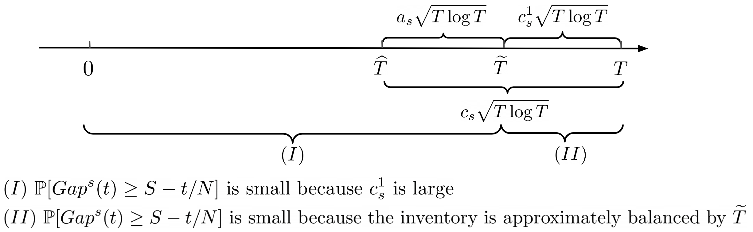
Figure 8: Illustration of $\widehat{T},\widetilde{T}$ and $T$

By construction, opaque selling starts at $\widehat{T}$. We leverage the definition of $\widetilde{T}$ to prove (51) by considering $t\leq\widetilde{T}$ and $t>\widetilde{T}$ separately. For $t\leq\widetilde{T}$,

$$\mathbb{P}(Gap^{s}(t)\geq S-t/N)=\mathbb{P}(\max_{j}x^{s}_{j}(t)\geq S)\leq\mathbb{P}(\max_{j}x^{s}_{j}(\widetilde{T})\geq S).$$

We make the following claim and defer its proof to Appendix B.2.3.

Claim 2.

$\mathbb{P}(\max_{j}x^{s}_{j}(\widetilde{T})\geq S)\leq\frac{a_{1}}{T^{2}}$ for some constant $a_{1}>0.$

Then, we have:

$$\sum_{t=S}^{N(S-1)+1}\mathbb{P}(Gap^{s}(t)\geq S-t/N) =\sum_{t=S}^{\widetilde{T}}\mathbb{P}(Gap^{s}(t)\geq S-t/N)+\sum_{t=\widetilde{T}+1}^{N(S-1)+1}\mathbb{P}(Gap^{s}(t)\geq S-t/N)$$

$$\leq T\cdot\frac{a_{1}}{T^{2}}+\sum_{t=\widetilde{T}+1}^{N(S-1)+1}\mathbb{P}(Gap^{s}(t)\geq S-t/N)$$

$$=\frac{a_{1}}{T}+\sum_{t=\widetilde{T}+1}^{N(S-1)+1}\mathbb{P}(Gap^{s}(t)\geq S-t/N).$$

Thus, it suffices to show that

$$\sum_{t=\widetilde{T}+1}^{N(S-1)+1}\mathbb{P}(Gap^{s}(t)\geq S-t/N)\leq a_{2},$$ (52)

for some constant $a_{2}>0$.

We now state the following lemma, whose proof is deferred to Appendix B.2.3.

Lemma 8.

Consider any policy $\pi$ that sets $\omega(t)=1$ when $t>t_{1}$, where $t_{1}\leq N(S-1)+1$. Define, for period $t_{2}$ such that $t_{1}\leq t_{2}\leq N(S-1)+1$, and for every $i$ and $j$

$$F_{ij}^{1} :=\left\{\sigma(t_{2})\in\Sigma(t_{2})\mid i\in\arg\max_{k\in[N]}x^{\mathcal{\pi}}_{k}(t_{2}),j\in\arg\min_{k\in[N]}x^{\mathcal{\pi}}_{k}(t_{2}),x^{\mathcal{\pi}}_{i}(t)\neq x^{\mathcal{\pi}}_{j}(t),\forall t\in\{t_{1},\chedit{...},t_{2}\}\right\}$$

$$F_{ij}^{2} :=\Big{\{}\sigma(t_{2})\in\Sigma(t_{2})\mid i\in\arg\max_{k\in[N]}x^{\mathcal{\pi}}_{k}(t_{2}),j\in\arg\min_{k\in[N]}x^{\mathcal{\pi}}_{k}(t_{2}),$$

$$\hskip 76.82234ptx^{\mathcal{\pi}}_{i}(t)=x^{\mathcal{\pi}}_{j}(t)\text{ for some }t\in\{t_{1},\chedit{...},t_{2}-1\},x^{\mathcal{\pi}}_{i}(t_{2})\neq x^{\mathcal{\pi}}_{j}(t_{2})\Big{\}}.$$

Then, there exists some constant $a_{3}>0$ such that

$$\sum_{t=t_{2}+1}^{N(S-1)+1}\mathbb{P}(Gap^{\pi}(t)\geq S-t/N)\leq a_{3}+\sum_{t=t_{2}+1}^{N(S-1)+1}\sum_{i,j}\mathbb{P}(F_{ij}^{1}).$$

Now, as in the balls-into-bins model, for $i,j\in[N]$, we define

$$E_{ij}^{1}:= \left\{\sigma(\widetilde{T})\in\Sigma(\widetilde{T})\mid i\in\arg\max_{k\in[N]}x^{s}_{k}(\widetilde{T}),j\in\arg\min_{k\in[N]}x^{s}_{k}(\widetilde{T}),x^{s}_{i}(t)\neq x^{s}_{j}(t),\forall t\in\{\widehat{T},\chedit{...},\widetilde{T}\}\right\}$$

$$E_{ij}^{2}:= \{\sigma(\widetilde{T})\in\Sigma(\widetilde{T})\mid i\in\arg\max_{k\in[N]}x^{s}_{k}(\widetilde{T}),j\in\arg\min_{k\in[N]}x^{s}_{k}(\widetilde{T}),$$

$$\hskip 76.82234ptx^{s}_{i}(t)=x^{s}_{j}(t)\text{ for some }t\in\{\widehat{T},\chedit{...},\widetilde{T}-1\},x^{s}_{i}(\widetilde{T})\neq x^{s}_{j}(\widetilde{T})\}$$

It follows that $E_{ij}^{1}$ and $E_{ij}^{2}$ satisfy the conditions for $F_{ij}^{1}$ and $F_{ij}^{2}$ in Lemma 8 with $t_{1}=\widehat{T}$ and $t_{2}=\widetilde{T}$. Thus, applying Lemma 8, we obtain

$$\sum_{t=\widetilde{T}+1}^{N(S-1)+1}\mathbb{P}(Gap^{s}(t)\geq S-t/N)\leq a_{3}+\sum_{t=\widetilde{T}+1}^{N(S-1)+1}\sum_{i,j}\mathbb{P}(E_{ij}^{1})$$ (53)

for some constant $a_{3}>0$.

To bound $\mathbb{P}(E_{ij}^{1})$, since $\widetilde{T}-\widehat{T}=a_{{s}}\sqrt{T\log(T)}\geq a_{{s}}\sqrt{\widetilde{T}\log(\widetilde{T})},$ we observe that $E_{ij}^{1}$ satisfies the condition for $F_{ij}^{1}$ in Lemma 4 with $t_{1}=\widehat{T}$ and $t_{2}=\widetilde{T}.$ Thus, applying Lemma 4, we obtain

$$\mathbb{P}\left(E_{ij}^{1}\right)\leq\beta\widehat{T}^{-2}+e^{-\alpha_{1}(\widetilde{T}-\widehat{T})}.$$

Since $\widehat{T}=T-c_{s}\sqrt{T\log(T)},$ there exists a constant $\beta_{1}$ such that $\mathbb{P}(E_{ij}^{1})\leq\beta_{1}T^{-2}+e^{-\alpha_{1}(\widetilde{T}-\widehat{T})}\ \forall\ i,j$, for large enough $T.$ Plugging this result back into (53), we obtain

$$\sum_{t=\widetilde{T}+1}^{N(S-1)+1}\mathbb{P}(Gap^{s}(t)\geq S-t/N) \leq a_{3}+\sum_{t=\widetilde{T}+1}^{N(S-1)+1}\sum_{i,j}(\beta_{1}T^{-2}+e^{-\alpha_{1}(\widetilde{T}-\widehat{T})})$$

$$\leq a_{3}+T\sum_{i,j}(\beta_{1}T^{-2}+e^{-\alpha_{1}(\widetilde{T}-\widehat{T})})\leq a_{2}$$

for some constant $a_{2}$ and large enough $T,$ where the second inequality comes from the fact that

$$N(S-1)+1-\widetilde{T}\leq N(S-1)+1=T.$$

∎

B.2.2 Proof of Corollary 1

Proof.

From Proposition 11 (iii), Proposition 12 (iii) and Proposition 13 (iii), we have

$$\mathcal{C}^{s} =\mathcal{K}^{s}+\mathcal{H}^{s}+\mathcal{D}^{s}\leq\frac{K}{NS-\theta_{s}}+\frac{h}{2}\left(NS+1+\theta_{s}\right)+\delta q\cdot\psi_{s},$$

where $\theta_{s}\in\mathcal{O}(1),\psi_{s}\in\Theta\left(\sqrt{\frac{\log S}{S}}\right)$. ∎

B.2.3 Proofs of Auxiliary Results

Proof of Lemma 8..

Suppose $F_{ij}^{2}$ occurs, and let $\tau=\max\{t\in\{t_{1},...,t_{2}-1\}\mid x^{\mathcal{\pi}}_{i}(t)=x^{\mathcal{\pi}}_{j}(t)\}.$ With slight abuse of notation, we denote by $F_{ij}^{2}\cap\tau$ the event that $F_{ij}^{2}$ occurs and $\tau$ is the last time that $x^{\mathcal{\pi}}_{i}(t)=x^{\mathcal{\pi}}_{j}(t)$.

For $t>t_{2}$, we have:

$$\begin{split}\mathbb{P}(Gap^{\pi}(t)\geq S-t/N)&=\mathbb{P}(Gap^{\pi}(t)\geq S-t/N\mid Gap^{\pi}(t_{2})=0)\cdot\mathbb{P}(Gap^{\pi}(t_{2})=0)\\ &\quad+\mathbb{P}(Gap^{\pi}(t)\geq S-t/N\mid Gap^{\pi}(t_{2})>0)\cdot\mathbb{P}(Gap^{\pi}(t_{2})>0)\\ &\leq\mathbb{P}(Gap^{\pi}(t)\geq S-t/N\mid Gap^{\pi}(t_{2})=0)\\ &\quad+\sum_{i,j}\left(\mathbb{P}(Gap^{\pi}(t)\geq S-t/N|F_{ij}^{1})\mathbb{P}(F_{ij}^{1})+\mathbb{P}(Gap^{\pi}(t)\geq S-t/N|F_{ij}^{2})\mathbb{P}(F_{ij}^{2})\right)\\ &\leq\underbrace{\mathbb{P}(Gap^{\pi}(t)\geq S-t/N\mid Gap^{\pi}(t_{2})=0)}_{(I)}\\ &\quad+\sum_{i,j}\left(\mathbb{P}(F_{ij}^{1})+\sum_{\tau=t_{1}}^{t_{2}}\mathbb{P}(Gap^{\pi}(t)\geq S-t/N|F_{ij}^{2}\cap\tau)\underbrace{\mathbb{P}(F_{ij}^{2}\cap\tau)}_{(II)}\right)\end{split}$$ (54)

Consider first $(I)$. Note that, conditional on $Gap^{\pi}(t_{2})=0$, policy $\pi$ takes the same actions as the always-flex policy would if it was initialized with all-empty bins at time $t_{2}$. (This observation will be re-used in the analyses that follow.) Thus, we have:

$$(I)=\mathbb{P}(Gap^{\pi}(t)\geq S-t/N\mid Gap^{\pi}(t_{2})=0)=\mathbb{P}(Gap^{a}(t-t_{2})\geq S-t/N),$$ (55)

Similarly, we can check that $F_{ij}^{2},t_{1}$ and $t_{2}$ satisfies the conditions in Lemma 5, which guarantees

$$(II)\leq\mathbb{P}(F_{ij}^{2}\mid t_{2}-\tau=t)\leq 4e^{-\alpha_{2}t}+e^{-\alpha_{3}t}.$$

Plugging these results back to (54) and summing over all $t>t_{2}$, we obtain

$$\sum_{t=t_{2}+1}^{N(S-1)+1}\mathbb{P}(Gap^{\pi}(t)\geq S-t/N) \leq\sum_{t=t_{2}+1}^{N(S-1)+1}\mathbb{P}(Gap^{a}(t-t_{2})\geq S-t/N)$$ (56)

$$\quad+\sum_{t=t_{2}+1}^{N(S-1)+1}\sum_{i,j}\mathbb{P}(F_{ij}^{1})$$

$$\quad+\sum_{t=t_{2}+1}^{N(S-1)+1}\sum_{i,j}\sum_{\tau=t_{1}}^{t_{2}}\mathbb{P}(Gap^{\pi}(t)\geq S-t/N|F_{ij}^{2}\cap\tau)$$

$$\qquad\qquad\times\left(4e^{-\alpha_{2}(t_{2}-\tau)}+e^{-\alpha_{3}(t_{2}-\tau)}\right).$$ (57)

We now bound each of these three terms. By Proposition 9, there exists some constant $a_{4}>0$ such that the first term is bounded above by

$$\sum_{t=t_{2}+1}^{N(S-1)+1}\mathbb{P}(Gap^{a}(t-t_{2})\geq S-t/N)\leq\sum_{t=t_{2}+1}^{N(S-1)+1}\beta e^{-c_{a}\cdot(S-t/N)}\leq a_{4}.$$

Moreover, for the third term, we can change the order of summation and obtain, for fixed $i$ and $j$:

$$\sum_{t=t_{2}+1}^{N(S-1)+1}\sum_{\tau=t_{1}}^{t_{2}}\mathbb{P}(Gap^{\pi}(t)\geq S-t/N|F_{ij}^{2}\cap\tau)\left(4e^{-\alpha_{2}(t_{2}-\tau)}+e^{-\alpha_{3}(t_{2}-\tau)}\right)$$

$$=\sum_{\tau=t_{1}}^{t_{2}}\left(4e^{-\alpha_{2}(t_{2}-\tau)}+e^{-\alpha_{3}(t_{2}-\tau)}\right)\sum_{t=t_{2}+1}^{N(S-1)+1}\mathbb{P}(Gap^{\pi}(t)\geq S-t/N|F_{ij}^{2}\cap\tau)$$ (58)

To bound (58), we formally state Claim 3 below and prove it in Appendix B.2.3.

Claim 3.

Consider any policy $\pi$ that sets $\omega(t)=1$ when $t>t_{2}$. Given $a>0$, let $F^{\prime}$ be any subset of the history before $t_{2}$ such that

$$F^{\prime}\subseteq F_{a}=\{\sigma(t_{2})\in\Sigma(t_{2})\mid Gap^{\pi}(t_{2})\leq a\}.$$

Then, $\mathbb{P}(Gap^{\pi}(t)\geq S-t/N\mid F^{\prime})\leq\mathbb{P}(Gap^{\pi}(t)\geq S-t/N-a\mid Gap^{\pi}(t_{2})=0)\ \forall\ t\geq t_{2}.$

By definition of $F_{ij}^{2}\cap\tau$, $Gap^{\pi}(t_{2})\leq t_{2}-\tau$, i.e., it satisfies the condition in Claim 3 with $F^{\prime}=F_{ij}^{2}\cap\tau,t_{2}$ and $a=t_{2}-\tau.$ Thus, we have

$$\mathbb{P}(Gap^{\pi}(t)\geq S-t/N\mid F_{ij}^{2}\cap\tau)\leq\mathbb{P}(Gap^{\pi}(t)\geq S-t/N-(t_{2}-\tau)\mid Gap^{\pi}(t_{2})=0),\forall t\geq t_{2}.$$

Plugging back (58) and Claim 3 into (57), we have:

$$\eqref{eq:part3} =\sum_{i,j}\sum_{t=t_{2}+1}^{N(S-1)+1}\sum_{\tau=t_{1}}^{t_{2}}\mathbb{P}(Gap^{\pi}(t)\geq S-t/N|F_{ij}^{2}\cap\tau)\left(4e^{-\alpha_{2}(t_{2}-\tau)}+e^{-\alpha_{3}(t_{2}-\tau)}\right)$$

$$\leq N^{2}\sum_{\tau=t_{1}}^{t_{2}}\left(4e^{-\alpha_{2}(t_{2}-\tau)}+e^{-\alpha_{3}(t_{2}-\tau)}\right)\sum_{t=t_{2}+1}^{N(S-1)+1}\mathbb{P}(Gap^{\pi}(t)\geq S-t/N-(t_{2}-\tau)\mid Gap^{\pi}(t_{2})=0)$$

$$\leq N^{2}\sum_{\tau=t_{1}}^{t_{2}}\left(4e^{-\alpha_{2}(t_{2}-\tau)}+e^{-\alpha_{3}(t_{2}-\tau)}\right)\sum_{t=t_{2}+1}^{N(S-1)+1}\mathbb{P}(Gap^{a}(t-t_{2})\geq S-t/N-(t_{2}-\tau))$$ (59)

$$\leq N^{2}\sum_{\tau=t_{1}}^{t_{2}}\left(4e^{-\alpha_{2}(t_{2}-\tau)}+e^{-\alpha_{3}(t_{2}-\tau)}\right)\left(\sum_{t=t_{2}+1}^{N[S-(t_{2}-\tau)]}\beta_{3}e^{-c_{a}(S-t/N-(t_{2}-\tau))}+\sum_{t=N[S-(t_{2}-\tau)]+1}^{N(S-1)+1}1\right)$$ (60)

$$\leq N^{2}\sum_{\tau=t_{1}}^{t_{2}}\left(4e^{-\alpha_{2}(t_{2}-\tau)}+e^{-\alpha_{3}(t_{2}-\tau)}\right)\left(a_{5}+N(t_{2}-\tau-1)+1\right)$$ (61)

$$\leq a_{6},$$

where $a_{5}$ and $a_{6}$ are positive constants. (59) follows from the same arguments as those used to establish (55). Then, in (60), since the application of Proposition 9 requires $S-t/N-(t_{2}-\tau)>0,$ we bound the $N(t_{2}-\tau-1)+1$ terms that do not satisfy this requirement by $1$ and the other terms by Proposition 9. Then, in obtaining (61) we observe that $\beta_{3}e^{-c_{a}(S-t/N-(t_{2}-\tau))}$, when ordered from $t=N[S-(t_{2}-\tau)]$ to $t=t_{2}+1$, is a decreasing sequence of exponentially small values whose sum converges to a positive constant $a_{5}$.

Then, putting (56) and (57) together, we have

$$\sum_{t=t_{2}+1}^{N(S-1)+1}\mathbb{P}(Gap^{\pi}(t)\geq S-t/N)\leq a_{3}+\sum_{t=t_{2}+1}^{N(S-1)+1}\sum_{i,j}\mathbb{P}(F_{ij}^{1}),$$

where $a_{3}:=a_{4}+a_{6}$, which is the bound in the lemma statement. ∎

Proof of Claim 2..

To prove the claim, we first show that

$$\mathbb{P}(\max_{j}x^{s}_{j}(\widetilde{T})\geq S)\leq\mathbb{P}(\max_{j}x^{nf}_{j}(\widetilde{T})\geq S-a_{{s}}\sqrt{T\log(T)}).$$ (62)

For (62), note that $\max_{j}x^{s}_{j}(\widetilde{T})\geq S$ implies $\max_{j}x^{s}_{j}(\widehat{T})\geq S-a_{{s}}\sqrt{T\log(T)}$, since in the worst case all balls from $\widehat{T}$ to $\widetilde{T}$ go into $\operatorname*{arg\,max}_{j}x^{s}_{j}(\widehat{T})$. Thus,

$$\mathbb{P}(\max_{j}x^{s}_{j}(\widetilde{T})\geq S)\leq\mathbb{P}(\max_{j}x^{s}_{j}(\widehat{T})\geq S-a_{{s}}\sqrt{T\log(T)}).$$

Since the no-flex policy and the static policy are the same before $\widehat{T},$ we also have:

$$\mathbb{P}(\max_{j}x^{s}_{j}(\widehat{T})\geq S-a_{{s}}\sqrt{T\log(T)}) =\mathbb{P}(\max_{j}x^{nf}_{j}(\widehat{T})\geq S-a_{{s}}\sqrt{T\log(T)})$$

$$\leq\mathbb{P}(\max_{j}x^{nf}_{j}(\widetilde{T})\geq S-a_{{s}}\sqrt{T\log(T)}),$$

where the inequality follows from the fact that $\widetilde{T}\geq\widehat{T}\implies\max_{j}x^{nf}_{j}(\widetilde{T})\geq\max_{j}x^{nf}_{j}(\widehat{T})$.

We now argue that

$$\mathbb{P}(\max_{j}x^{nf}_{j}(\widetilde{T})\geq S-a_{{s}}\sqrt{T\log(T)})\leq\frac{a_{1}}{T^{2}}$$ (63)

for some constant $a_{1}>0$ to conclude the proof of the claim.

Recall, $c_{s}^{1}=\frac{2\sqrt{6}N(N-1)N}{q}+4N$ and $a_{{s}}=\frac{2\sqrt{6}N(N-1)}{q}$, so $c_{s}^{1}=N(a_{{s}}+4).$ For large enough $T,$

$$\mathbb{P}(\max_{j}x^{nf}_{j}(\widetilde{T})\geq S-a_{{s}}\sqrt{T\log(T)}) \leq N\mathbb{P}\left(B(T-c_{s}^{1}\sqrt{T\log(T)},\frac{1}{N})\geq\frac{T-N\cdot a_{{s}}\sqrt{T\log(T)}}{N}\right)$$

$$=N\mathbb{P}\left(B(T-c_{s}^{1}\sqrt{T\log(T)},\frac{1}{N})\geq(1+\epsilon)\frac{T-c_{s}^{1}\sqrt{T\log(T)}}{N}\right),$$ (64)

where

$$\epsilon=\frac{(c_{s}^{1}-Na_{{s}})\sqrt{T\log(T)}}{T-c_{s}^{1}\sqrt{T\log(T)}}=\frac{4N\sqrt{T\log T}}{T-c_{static}^{1}\sqrt{T\log T}}.$$

The first inequality above follows from $SN>T=N(S-1)+1,$ which yields

$$S-a_{{s}}\sqrt{T\log(T)}=\frac{NS-N\cdot a_{{s}}\sqrt{T\log(T)}}{N}\geq\frac{T-N\cdot a_{{s}}\sqrt{T\log(T)}}{N}.$$

Then, applying the Chernoff bound to (64) we obtain:

$$\mathbb{P}(\max_{j}x^{nf}_{j}(\widetilde{T})\geq S-a_{{s}}\sqrt{T\log(T)}) \leq\exp\left(-\frac{\epsilon^{2}}{2+\epsilon}\frac{T-c_{s}^{1}\sqrt{T\log(T)}}{N}\right)$$

$$=\exp\left(-\frac{(c_{s}^{1}-Na_{{s}})^{2}T\log(T)}{2N(T-c_{s}^{1}\sqrt{T\log(T)})+N(c_{s}^{1}-Na_{{s}})\sqrt{T\log(T)}}\right)$$

$$\leq\exp\left(-\frac{16N^{2}T\log(T)}{2NT+4N^{2}\sqrt{T\log(T)}}\right)$$

$$\leq e^{-\frac{16\log(T)}{6}}\leq\frac{a_{1}}{T^{2}}$$

for some constant $a_{1}>0.$ For the second inequality above we plug in values of $c_{s}^{1}$, $a_{{s}}$, and upper bound $(T-c_{s}^{1}\sqrt{T\log(T)})$ by $T.$ ∎

Proof of Claim 3..

We first construct two bin configurations at $t_{2}$. Let $x^{\text{fic}}_{k}(t_{2})=t_{2}/N+a,\forall k\in[N].$ Then, consider any sample path

$$\sigma^{\prime}(t_{2})\in F^{\prime}\subseteq F_{a}=\{\sigma(t_{2})\in\Sigma(t_{2})\mid Gap^{\pi}(t_{2})\leq a\text{ for some a}\geq 0\}$$

and denote the loads corresponding to $\sigma^{\prime}(t_{2})$ at $t_{2}$ by $x^{\text{real}}_{k}(t_{2}),\forall k\in[N].$ In both of these two configurations balls follow $\omega(t)=1,\forall t>t_{2}$, so we assume the same realization of randomness, i.e., the same $f(t),P(t)$ and $F(t)\;\forall t\geq t_{2}$. We shall show that, for any $\sigma^{\prime}(t_{2})\in F^{\prime}$, we have

$$x^{\text{real}}_{k}(t)\leq x^{\text{fic}}_{k}(t),\forall t\geq t_{2},\forall k\in[N],$$ (65)

as long as both $x^{\text{real}}_{k}(t)$ and $x^{\text{fic}}_{k}(t)$ develop based on the static policy being applied to the same arrivals $\theta({t_{2}}),\ldots,\theta({t})$. Assuming this holds, then, for any $\sigma^{\prime}(t_{2})\in F^{\prime}$ we have

$$\max_{k}x^{\text{real}}_{k}(t)-t/N\leq\max_{k}x^{\text{fic}}_{k}(t)-t/N\;\forall t\geq t_{2}$$

assuming the same realization of randomness. This would then imply:

$$\mathbb{P}(Gap^{\pi}(t)\geq S-t/N|F^{\prime}) =\sum_{\sigma^{\prime}(t_{2})\in F^{\prime}}\mathbb{P}(\max_{k}x^{\text{real}}_{k}(t)-t/N\geq S-t/N\mid\sigma^{\prime}(t_{2}))\mathbb{P}(\sigma^{\prime}(t_{2}))$$

$$\leq\sum_{\sigma^{\prime}(t_{2})\in F^{\prime}}\mathbb{P}(\max_{k}x^{\text{fic}}_{k}(t)-t/N\geq S-t/N\mid\sigma^{\prime}(t_{2}))\mathbb{P}(\sigma^{\prime}(t_{2}))$$

$$=\mathbb{P}(\max_{k}x^{\text{fic}}_{k}(t)-t/N\geq S-t/N)$$

$$\leq\mathbb{P}(Gap^{\pi}(t)+a\geq S-t/N\mid Gap^{\pi}(t_{2})=0)$$

$$=\mathbb{P}(Gap^{\pi}(t)\geq S-t/N-a\mid Gap^{\pi}(t_{2})=0),\forall t\geq t_{2}.$$

What is left to conclude the proof is inequality (65), which we now show by induction.

Base case: $t=t_{2}$. For this case we get from the definitions of $F^{\prime}$ and $x^{\text{fic}}(t_{2})$ that

$$x^{\text{real}}_{k}(t_{2})\leq\max_{k^{\prime}}x^{\text{real}}_{k^{\prime}}(t_{2})\leq t_{2}/N+a=x^{\text{fic}}_{k}(t_{2}),\forall k\in[N].$$

Inductive step. Fix $t\in\{t_{2}+1,\ldots,T\}$, and suppose $x^{\text{real}}_{k}(t)\leq x^{\text{fic}}_{k}(t),\forall k\in[N].$ We show that $x^{\text{real}}_{k}(t+1)\leq x^{\text{fic}}_{k}(t+1),\forall k\in[N],$ by discussing the following cases.

1. Suppose $f(t)=0$ and $P(t)=k_{1}\in[N]$. Under such an arrival we have

   $$x^{\text{real}}_{k_{1}}(t+1)=x^{\text{real}}_{k_{1}}(t)+1\text{ and }x^{\text{fic}}_{k_{1}}(t+1)=x^{\text{fic}}_{k_{1}}(t)+1,$$

   while the loads of other bins do not change. Thus, $x^{\text{real}}_{k}(t+1)\leq x^{\text{fic}}_{k}(t+1),\forall k\in[N].$

2. Suppose $f(t)=1$, with $F(t)=\{k_{1},k_{2}\}$, for some $k_{1},k_{2}\in[N]$.

   1. If $x^{\text{fic}}_{k_{1}}(t)<x^{\text{fic}}_{k_{2}}(t)$ then a flex ball lands in bin $k_{1}$ in the fictional configuration. If the flex ball also goes into bin $k_{1}$ in the real configuration, the induction holds. Else, i.e., if the flex ball goes into bin $k_{2}$ in the real allocation, then it must be the case that $x^{\text{real}}_{k_{2}}(t)\leq x^{\text{real}}_{k_{1}}(t)$, which implies that

      $$x^{\text{real}}_{k_{2}}(t)\leq x^{\text{real}}_{k_{1}}(t)\leq x^{\text{fic}}_{k_{1}}(t)<x^{\text{fic}}_{k_{2}}(t).$$

      The induction also holds in this case because

      $$x^{\text{real}}_{k_{2}}(t+1)=x^{\text{real}}_{k_{2}}(t)+1\leq x^{\text{fic}}_{k_{2}}(t)=x^{\text{fic}}_{k_{2}}(t+1),$$

      and all other bin loads remain unchanged.

   2. For $x^{\text{fic}}_{k_{1}}(t)>x^{\text{fic}}_{k_{2}}(t)$, an argument symmetric to case 2.1 shows that the induction holds.

   3. If $x^{\text{fic}}_{k_{1}}(t)=x^{\text{fic}}_{k_{2}}(t)$ and $k_{1}<k_{2}$, then a flex ball goes into bin $k_{1}$ in the fictional configuration. In this case, if $x^{\text{real}}_{k_{1}}(t)\leq x^{\text{real}}_{k_{2}}(t)$ then the flex ball would go into bin $k_{1}$ in the real allocation and the induction still holds. Else, i.e., if $x^{\text{real}}_{k_{1}}(t)>x^{\text{real}}_{k_{2}}(t)$, then the flex ball goes into bin $k_{2}$. In that scenario we must have

      $$x^{\text{real}}_{k_{2}}(t)<x^{\text{real}}_{k_{1}}(t)\leq x^{\text{fic}}_{k_{1}}(t)=x^{\text{fic}}_{k_{2}}(t).$$

      This leads to

      $$x^{\text{real}}_{k_{2}}(t+1)=x^{\text{real}}_{k_{2}}(t)+1\leq x^{\text{fic}}_{k_{2}}(t)=x^{\text{fic}}_{k_{2}}(t+1),$$

      and all other bin loads remain unchanged, so the induction still holds in this case. We omit the proof for the case where $k_{1}>k_{2}$, as it is symmetric.

∎

B.3 Analysis of the dynamic opaque selling policy

B.3.1 Proof of Theorem 6

Proof.

Applying Proposition 10 to the dynamic policy, we obtain

$$\mathbb{E}[R^{d}]=N(S-1)+2-\sum_{t=S}^{N(S-1)+1}\mathbb{P}(Gap^{d}(t)\geq S-t/N).$$

Thus, to prove Theorem 6, it suffices to show that $\sum_{t=S}^{N(S-1)+1}\mathbb{P}(Gap^{d}(t)\geq S-t/N)\in\mathcal{O}(1).$

Recall that $c_{d}=\frac{1}{10\binom{N}{2}}$ and define $T^{\star}=\inf\{t\,:\,Gap^{d}(t)\geq\frac{c_{d}(T-t)q}{N}\}$. By definition, the policy always attempts to flex after $T^{\star}$, but never before. Moreover, as illustrated in Fig. 9, we define $\widetilde{T}:=T^{\star}+\frac{T-T^{\star}}{2}$, i.e., $\widetilde{T}$ is the mid-point of $T$ and $T^{\star}$.

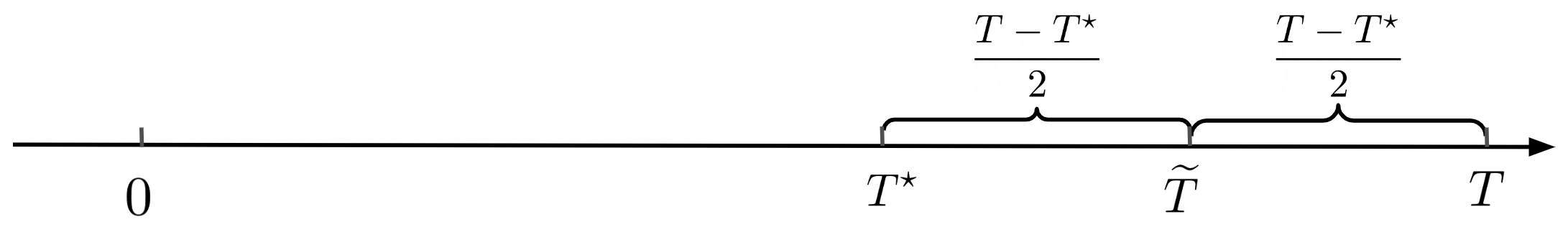
Figure 9: Illustration of $T^{\star},\widetilde{T}$ and $T$

Since $T=N(S-1)+1$, one can verify that $\frac{c_{d}(T-t)q}{N}<S-t/N$ for all $t\leq T$. Thus, given $T^{\star}$:

$$Gap^{d}(t)<\frac{c_{d}(T-t)q}{N}\quad\forall\,t<T^{\star}\implies Gap^{d}(t)<S-t/N\quad\forall\,t<T^{\star},$$

and as a result:

$$\sum_{t=S}^{N(S-1)+1}\mathbb{P}\left(Gap^{d}(t)\geq S-t/N\mid\,T^{\star}\right) =\sum_{t=T^{\star}}^{N(S-1)+1}\mathbb{P}\left(Gap^{d}(t)\geq S-t/N\,\mid\,T^{\star}\right)$$ (66)

$$=\underbrace{\sum_{t=T^{\star}}^{\widetilde{T}}\mathbb{P}\left(Gap^{d}(t)\geq S-t/N\,\mid\,T^{\star}\right)}_{(I)}$$

$$\qquad+\underbrace{\sum_{t=\widetilde{T}+1}^{N(S-1)+1}\mathbb{P}\left(Gap^{d}(t)\geq S-t/N\,\mid\,T^{\star}\right)}_{(II)}.$$

We show that for any value of $T^{\star}$ each of these two terms is upper bounded by a constant, which will complete the proof.

Step 1: Bound $(I)$

Consider first $(I)$, and let $E_{T^{\star}}$ denote the event that $Gap^{d}(T^{\star})<\frac{c_{d}(T-T^{\star})q}{N}+\frac{c_{d}q}{N}+1$. Putting together the facts that: (i) $Gap^{d}(T^{\star}-1)<\frac{c_{d}(T-(T^{\star}-1))q}{N}$ by definition, and (ii) $Gap^{d}(T^{\star})\leq Gap^{d}(T^{\star}-1)+1$, we have:

$$Gap^{d}(T^{\star})\leq\frac{c_{d}(T-T^{\star})q}{N}+\frac{c_{d}q}{N}+1.$$ (67)

Thus, $\mathbb{P}\left(E_{T^{\star}}\right)=1$, and:

$$(I) =\sum_{t=T^{\star}}^{\widetilde{T}}\mathbb{P}(Gap^{d}(t)\geq S-t/N\,\mid\,Gap^{d}(T^{\star})<\frac{c_{d}(T-T^{\star})q}{N}+\frac{c_{d}q}{N}+1,T^{\star})$$

Further, $(I)$ satisfies the condition in Claim 3 with $F^{\prime}=E_{T^{\star}},t_{2}=T^{\star}$ and $a=\frac{c_{d}(T-T^{\star})q}{N}+\frac{c_{d}q}{N}+1.$ Thus, from Claim 3 we have

$$\mathbb{P}(Gap^{d}(t)\geq S-t/N\,\mid\,Gap^{d}(T^{\star})<\frac{c_{d}(T-T^{\star})q}{N}+\frac{c_{d}q}{N}+1,T^{\star})$$

$$\leq\mathbb{P}\left(Gap^{d}(t)\geq S-t/N-\left(\frac{c_{d}(T-T^{\star})q}{N}+\frac{c_{d}q}{N}+1\right)\,\mid\,Gap^{d}(T^{\star})=0,T^{\star}\right),\forall t\geq T^{\star}.$$

Then, we have:

$$(I) \leq\sum_{t=T^{\star}}^{\widetilde{T}}\mathbb{P}\left(Gap^{d}(t)\geq S-t/N-\left(\frac{c_{d}(T-T^{\star})q}{N}+\frac{c_{d}q}{N}+1\right)\,\mid\,Gap^{d}(T^{\star})=0,T^{\star}\right)$$

$$\leq\sum_{t=T^{\star}}^{\widetilde{T}}\mathbb{P}\left(Gap^{a}(t-T^{\star})\geq S-t/N-\left(\frac{c_{d}(T-T^{\star})q}{N}+\frac{c_{d}q}{N}+1\right)\mid T^{\star}\right)$$ (68)

(68) again follows from the observation that, conditional on $Gap^{d}(T^{\star})=0,$ our dynamic policy takes the same action as the always-flex policy beginning at $T^{\star}.$

Let $\widetilde{T}:=T^{\star}+\frac{T-T^{\star}}{2}$, i.e., $\widetilde{T}$ is the mid-point of $T$ and $T^{\star}$. We have:

$$S-\frac{t}{N}-\left(\frac{c_{d}(T-T^{\star})q}{N}+\frac{c_{d}q}{N}+1\right) =S-\frac{\widetilde{T}}{N}-\left(\frac{c_{d}(T-T^{\star})q}{N}+\frac{c_{d}q}{N}+1\right)+\frac{\widetilde{T}-t}{N}$$

$$=S-\frac{T^{\star}+\frac{T-T^{\star}}{2}}{N}-(\frac{c_{d}(T-T^{\star})q}{N}+\frac{c_{d}q}{N}+1)+\frac{\widetilde{T}-t}{N}$$

$$\geq\frac{T-T^{\star}}{N}(\frac{1}{2}-c_{d}q)-\frac{c_{d}q}{N}+1+\frac{\widetilde{T}-t}{N}.$$

The inequality above follows from:

$$S-\frac{T^{\star}+\frac{T-T^{\star}}{2}}{N}=\frac{NS-T^{\star}}{N}-\frac{T-T^{\star}}{2N}\geq\frac{T-T^{\star}}{N}-\frac{T-T^{\star}}{2N}=\frac{T-T^{\star}}{N}\frac{1}{2}.$$

Using this, we upper bound $(I)$ as follows:

$$\begin{split}(I)&\leq\sum_{t=T^{\star}}^{\widetilde{T}}\mathbb{P}(Gap^{a}(t-T^{\star})\geq S-t/N-(\frac{c_{d}(T-T^{\star})q}{N}+\frac{c_{d}q}{N}+1)\,\mid\,T^{\star})\\ &\leq\sum_{t=T^{\star}}^{\widetilde{T}-c_{d}q}\mathbb{P}(Gap^{a}(t-T^{\star})\geq S-t/N-(\frac{c_{d}(T-T^{\star})q}{N}+\frac{c_{d}q}{N}+1)\,\mid\,T^{\star})+\sum_{t=\widetilde{T}-c_{d}q+1}^{\widetilde{T}}1\\ &\leq\sum_{t=T^{\star}}^{\widetilde{T}-c_{d}q}\beta e^{-c_{a}[S-t/N-(\frac{c_{d}(T-T^{\star})q}{N}+\frac{c_{d}q}{N}+1)]}+c_{d}q\\ &\leq a_{1}\end{split}$$

for some constant $a_{1}$ (that is independent of $T^{\star}$). We may assume without loss of generality that $\widetilde{T}-c_{semi}q$ is an integer since this changes our constant bound by at most $1$. For the third inequality above, we apply Proposition 9 again. Finally, in the last inequality we observe that

$$\frac{1}{2}-c_{d}q=\frac{1}{2}-\frac{q}{10\binom{N}{2}}>0,$$

and thus

$$S-t/N-\left(\frac{c_{d}(T-T^{\star})q}{N}+\frac{c_{d}q}{N}+1\right)\geq\frac{T-T^{\star}}{N}\left(\frac{1}{2}-c_{d}q\right)-\frac{c_{d}q}{N}+1+\frac{\widetilde{T}-t}{N}\geq 0,\forall t\leq\widetilde{T}-c_{d}q.$$

Thus, $\beta e^{-c_{a}[S-t/N-(\frac{c_{d}(T-T^{\star})q}{N}+\frac{c_{d}q}{N}+1)]}$, when ordered from $t=\widetilde{T}-c_{d}q$ to $t=T^{\star}$, is a decreasing sequence of exponentially small values, and its sum converges to a positive constant.

Step 2: Bound $(II)$

Now, to bound $(II)$, we re-define, for $i,j\in[N]$,

$$E_{ij}^{1} :=\left\{\sigma(\widetilde{T})\in\Sigma(\widetilde{T})\mid i\in\arg\max_{k\in[N]}x^{d}_{k}(\widetilde{T}),j\in\arg\min_{k\in[N]}x^{d}_{k}(\widetilde{T}),x^{d}_{i}(t)\neq x^{d}_{j}(t),\forall t\in\{T^{\star},\chedit{...},\widetilde{T}\}\right\}$$

$$E_{ij}^{2} :=\{\sigma(\widetilde{T})\in\Sigma(\widetilde{T})\mid i\in\arg\max_{k\in[N]}x^{d}_{k}(\widetilde{T}),j\in\arg\min_{k\in[N]}x^{d}_{k}(\widetilde{T}),x^{d}_{i}(t)=x^{d}_{j}(t)\text{ for some }t\in\{T^{\star},\chedit{...},\widetilde{T}-1\},$$

$$\hskip 85.35826ptx^{d}_{i}(\widetilde{T})\neq x^{d}_{j}(\widetilde{T})\}$$

$E_{ij}^{1}$ and $E_{ij}^{2}$ above satisfy the conditions for $F_{ij}^{1}$ and $F_{ij}^{2}$ in Lemma 8 with $t_{1}=T^{\star}$ and $t_{2}=\widetilde{T}$. Thus, applying Lemma 8, we obtain

$$\sum_{t=\widetilde{T}+1}^{N(S-1)+1}\mathbb{P}(Gap^{d}(t)\geq S-t/N\mid T^{\star})\leq a_{3}+\sum_{t=\widetilde{T}+1}^{N(S-1)+1}\sum_{i,j}\mathbb{P}(E_{ij}^{1}\mid T^{\star})$$ (69)

for some constant $a_{3}.$ To bound $\mathbb{P}(E_{ij}^{1}\mid T^{\star})$, recall from (33) that $\max_{k}x^{d}_{k}(T^{\star})-\min_{k}x^{d}_{k}(T^{\star})\leq NGap^{d}(T^{\star}).$ By (67), we obtain

$$\max_{k}x^{d}_{k}(T^{\star})-\min_{k}x^{d}_{k}(T^{\star}) \leq N(\frac{c_{d}(T-T^{\star})q}{N}+\frac{c_{d}q}{N}+1)$$

$$=c_{d}(T-T^{\star})q+c_{d}q+N$$

$$=2c_{d}(\widetilde{T}-T^{\star})q+c_{d}q+N$$

$$=\frac{1}{5\binom{N}{2}}(\widetilde{T}-T^{\star})q+c_{d}q+N.$$ (70)

Thus, $E_{ij}^{1}$ satisfies the definition of $F_{ij}^{1}$ in Lemma 6, with $t_{1}=T^{\star}$ and $t_{2}=\widetilde{T}.$ Moreover, from (70), with $a_{p}=\frac{1}{5\binom{N}{2}}$ and $a=c_{d}q+N$ we satisfy all conditions in Lemma 6, and there exist constants $\alpha_{0},\alpha_{1}$ and $t_{0}$ such that

$$\mathbb{P}(E_{ij}^{1}\mid T^{\star})\leq 4e^{-\alpha_{0}(\widetilde{T}-T^{\star})}+e^{-\alpha_{1}(\widetilde{T}-T^{\star})}\quad\forall\widetilde{T}-T^{\star}\geq t_{0}.$$

Since $\widetilde{T}-T^{\star}=\frac{1}{2}(T-T^{\star})$, we then have

$$\mathbb{P}(E_{ij}^{1}\mid T^{\star})\leq 4e^{-\frac{\alpha_{0}}{2}(T-T^{\star})}+e^{-\frac{\alpha_{1}}{2}(T-T^{\star})}\quad\forall T-T^{\star}\geq 2t_{0}.$$

Plugging this result back to (69), we obtain

$$(II)=\sum_{t=\widetilde{T}+1}^{N(S-1)+1}\mathbb{P}(Gap^{d}(t)\geq S-t/N\mid T^{\star}) \leq a_{3}+\sum_{t=\widetilde{T}+1}^{N(S-1)+1}\sum_{i,j}(4e^{-\frac{\alpha_{0}}{2}(T-T^{\star})}+e^{-\frac{\alpha_{1}}{2}(T-T^{\star})})$$

$$\leq a_{3}+\sum_{i,j}(T-T^{\star})(4e^{-\frac{\alpha_{0}}{2}(T-T^{\star})}+e^{-\frac{\alpha_{1}}{2}(T-T^{\star})})$$

$$\leq a_{2}\qquad\forall\,T-T^{\star}\geq 2t_{0}$$

for some constant $a_{2}$, where the second inequality comes from the fact that

$$N(S-1)+1-\widetilde{T}=T-\widetilde{T}\leq T-T^{\star}.$$

Then, $\sum_{t=S}^{N(S-1)+1}\mathbb{P}\left(Gap^{d}(t)\geq S-t/N\mid\,T^{\star}\right)=(I)+(II)\leq a_{1}+a_{2}\forall T-T^{\star}\geq 2t_{0}.$ Recall from (66) that

$$\sum_{t=S}^{N(S-1)+1}\mathbb{P}\left(Gap^{d}(t)\geq S-t/N\mid\,T^{\star}\right)=\sum_{t=T^{\star}}^{N(S-1)+1}\mathbb{P}\left(Gap^{d}(t)\geq S-t/N\right).$$

Thus, for $T-T^{\star}<2t_{0}$ we have

$$\sum_{t=S}^{N(S-1)+1}\mathbb{P}\left(Gap^{d}(t)\geq S-t/N\mid\,T^{\star}\right)=\sum_{t=T^{\star}}^{N(S-1)+1}1\leq 2t_{0},$$

which completes the proof. ∎

B.3.2 Proof of Corollary 2

Proof.

From Proposition 11 (iv), Proposition 12 (iv) and Proposition 13 (iv), we have

$$\mathcal{C}^{d} =\mathcal{K}^{d}+\mathcal{H}^{d}+\mathcal{D}^{d}\leq\frac{K}{NS-\theta_{d}}+\frac{h}{2}\left(NS+1+\theta_{d}\right)+\delta q\cdot\psi_{d},$$

where $\theta_{d}\in\mathcal{O}(1),\psi_{d}\in\mathcal{O}\left(\frac{1}{\sqrt{S}}\right)$. ∎

B.4 Benchmark comparisons

B.4.1 Proof of Proposition 3

Proof.

Recall, from (1), that

$$\mathcal{C}^{\pi}=\frac{K}{\mathbb{E}\left[R^{\pi}\right]}+\frac{h}{2}\left(2NS+1-\frac{\mathbb{E}\left[(R^{\pi})^{2}\right]}{\mathbb{E}\left[R^{\pi}\right]}\right)+\frac{\mathbb{E}\left[D^{\pi}\right]}{\mathbb{E}\left[R^{\pi}\right]}\cdot\delta \geq\frac{K}{\mathbb{E}\left[R^{\pi}\right]}+\frac{h}{2}\left(2NS+1-\mathbb{E}\left[R^{\pi}\right]\right)$$

$$\geq\frac{K}{N(S-1)+1}+\frac{h}{2}(NS+N)$$

where the first inequality follows from Jensen’s inequality for the second term, and non-negative discount costs for the third. Noting that $R^{\pi}\leq N(S-1)+1$ for all $\pi$, we obtain the last inequality. ∎

B.4.2 Proof of Proposition 6

Proof.

From Proposition 11 (i), Proposition 12 (i) Proposition 13 (i) we have

$$\mathcal{C}^{nf}\geq\frac{K}{NS-\theta_{nf}}+h\frac{(NS)^{2}-\frac{NS}{2}\theta_{nf}}{2(NS-\theta_{nf})},\text{ where }\theta_{nf}\in\Omega(\sqrt{S}).$$

Since

$$\mathcal{C}^{s}\leq\frac{K}{NS-\theta_{s}}+\frac{h}{2}\left(NS+1+\theta_{s}\right)+\delta q\cdot\psi_{s},\text{ where }\theta_{s}\in\mathcal{O}(1),\psi_{s}\in\Theta(\sqrt{\frac{\log(S)}{S}}),$$

by Corollary 1, we have

$$\mathcal{C}^{nf}-\mathcal{C}^{s} \geq K\cdot\frac{\theta_{nf}-\theta_{s}}{(NS-\theta_{nf})(NS-\theta_{s})}+\frac{h}{2}\frac{NS(\frac{\theta_{nf}}{2}-\theta_{s}-1)+\theta_{nf}+\theta_{nf}\theta_{s}}{(NS-\theta_{nf})}-\delta q\cdot\psi_{s}$$

$$\geq K\cdot\frac{\theta_{nf}-\theta_{s}}{(NS)^{2}}+\frac{h}{2}\frac{NS(\frac{\theta_{nf}}{2}-\theta_{s}-1)}{NS}-\delta q\cdot\psi_{s}$$

Similarly, from Proposition 11 (ii), Proposition 12 (ii) Proposition 13 (ii):

$$\mathcal{C}^{a}\geq\frac{K}{NS}+\frac{h}{2}N(S+1)+\delta\cdot q.$$

Thus,

$$\mathcal{C}^{a}-\mathcal{C}^{s} \geq-K\frac{\theta_{s}}{NS(NS-\theta_{s})}-\frac{h}{2}(\theta_{s}-N+1)+\delta q(1-\psi_{s})\geq-K\frac{\theta_{s}}{(NS)^{2}}-\frac{h}{2}\theta_{s}+\delta q(1-\psi_{s}).$$

Finally, plugging in the definition of $\mathcal{C}^{\star}$,

$$\mathcal{C}^{\star}-\mathcal{C}^{s}\geq-K\frac{\theta_{s}}{(NS)^{2}}-\frac{h}{2}\theta_{s}-\delta q\cdot\psi_{s}.$$

∎

B.4.3 Proof of Proposition 7

Proof.

By Corollary 2:

$$\mathcal{C}^{d} \leq\frac{K}{NS-\theta_{d}}+\frac{h}{2}\left(NS+1+\theta_{d}\right)+\delta q\,\psi_{d},\text{ where }\theta_{d}\in\mathcal{O}(1),\psi_{d}\in\mathcal{O}\left(\frac{1}{\sqrt{S}}\right)$$

$$\implies\mathcal{C}^{nf}-\mathcal{C}^{d} \geq K\cdot\frac{\theta_{nf}-\theta_{d}}{(NS-\theta_{nf})(NS-\theta_{d})}+\frac{h}{2}\frac{NS(\frac{\theta_{nf}}{2}-\theta_{d}-1)+\theta_{nf}+\theta_{nf}\theta_{d}}{(NS-\theta_{nf})}-\delta q\cdot\psi_{d}$$

$$\geq K\cdot\frac{\theta_{nf}-\theta_{d}}{(NS)^{2}}+\frac{h}{2}\frac{NS(\frac{\theta_{nf}}{2}-\theta_{d}-1)}{NS}-\delta q\cdot\psi_{d}.$$

Similarly,

$$\mathcal{C}^{a}-\mathcal{C}^{d} \geq-K\frac{\theta_{d}}{NS(NS-\theta_{d})}-\frac{h}{2}(\theta_{d}-N+1)+\delta q(1-\psi_{d})\geq-K\frac{\theta_{d}}{(NS)^{2}}-\frac{h}{2}\theta_{d}+\delta q(1-\psi_{d}),$$

and

$$\mathcal{C}^{\star}-\mathcal{C}^{d}\geq-K\frac{\theta_{d}}{(NS)^{2}}-\frac{h}{2}\theta_{d}-\delta q\cdot\psi_{d}.$$

∎

B.4.4 Proof of Corollary 3

Proof.

By Proposition 11 (iii), Proposition 12 (iii) Proposition 13 (iii):

$$\mathcal{C}^{s}\geq\frac{K}{NS}+\frac{h}{2}N(S+1)+\delta q\cdot\psi_{s}\implies\mathcal{C}^{s}-\mathcal{C}^{d}\geq-K\frac{\theta_{d}}{(NS)^{2}}-\frac{h}{2}\theta_{d}+\delta q(\psi_{s}-\psi_{d}).$$

∎

B.4.5 Proof of Theorem 4

Proof.

For the dynamic policy, based on Corollary 2 we can bound

$$\mathcal{C}^{d}-\mathcal{C}^{\star} =\mathcal{K}^{d}+\mathcal{H}^{d}+\mathcal{D}^{d}-\frac{K}{N(S-1)+1}-\frac{h}{2}(NS+N)$$

$$\leq K\left(\frac{1}{NS-\theta_{d}}-\frac{1}{N(S-1)+1}\right)+\frac{h}{2}\left(NS+1+\theta_{d}-NS-N\right)+\delta q\psi_{d}$$

where $\theta_{d}\in\mathcal{O}(1)$ and $\psi_{d}\in\mathcal{O}\left(\frac{1}{\sqrt{S}}\right).$ This expression simplifies to

$$\mathcal{C}^{d}-\mathcal{C}^{\star}\leq\Theta\left(\frac{1}{S}\right)+\delta q\mathcal{O}\left(\frac{1}{\sqrt{S}}\right).$$

Thus, when $\delta\in\mathcal{O}\left(\frac{1}{\sqrt{S}}\right),$ we have $\mathcal{C}^{d}-\mathcal{C}^{\star}\leq\mathcal{O}\left(\frac{1}{S}\right),$ which completes the proof of part (i).

For part (ii), with $\delta\in\mathcal{O}(1),$ the expression simplifies to

$$\mathcal{C}^{d}-\mathcal{C}^{\star}\leq\mathcal{O}\left(\frac{1}{\sqrt{S}}\right).$$

Thus, we first show that the no-flex policy incurs $\Omega\left(\frac{1}{\sqrt{S}}\right)$ loss relative to OPT, and then compare the dynamic policy to the static and the always-flex policy.

For the no-flex policy, we have from Proposition 11 (i), Proposition 12 (i) and Proposition 13 (i):

$$\mathcal{C}^{nf}-\mathcal{C}^{\star} =\mathcal{K}^{nf}+\mathcal{H}^{nf}+\mathcal{D}^{nf}-\frac{K}{N(S-1)+1}-\frac{h}{2}(NS+N)$$

$$\geq K\left(\frac{1}{NS-\theta_{nf}}-\frac{1}{N(S-1)+1}\right)+\frac{h}{2}\left(\frac{(NS)^{2}-\frac{NS}{2}\theta_{nf}+\mathcal{O}(N^{2}S)}{NS-\theta_{nf}}-NS-N\right)$$

$$=K\frac{\theta_{nf}-N+1}{(NS-\theta_{nf})(N(S-1)+1)}+\frac{h}{2}\frac{\frac{NS}{2}\theta_{nf}-N^{2}S+N\theta_{nf}+\mathcal{O}(N^{2}S)}{NS-\theta_{nf}}$$

$$\geq K\frac{\theta_{nf}}{(NS)^{2}}+\frac{h}{2}\frac{\frac{NS}{2}\theta_{nf}}{NS}-\frac{h}{2}\frac{N^{2}S-N\theta_{nf}-\mathcal{O}(N^{2}S)}{NS},$$

where $\theta_{nf}\in\Omega(\sqrt{S}).$ Substituting for $K$ and $h$, the above simplifies to $\Omega(\frac{1}{\sqrt{S}})+\Omega(\frac{1}{\sqrt{S}})-\mathcal{O}(\frac{1}{S}).$ Thus,

$$\mathcal{C}^{nf}-\mathcal{C}^{\star}\geq\Omega(\frac{1}{\sqrt{S}}).$$

Then, for the flexing policies, based on Proposition 3 we can lower bound

$$\mathcal{C}^{a}-\mathcal{C}^{\star} =\mathcal{K}^{a}+\mathcal{H}^{a}+\mathcal{D}^{a}-\frac{K}{N(S-1)+1}-\frac{h}{2}(NS+N)\geq\mathcal{D}^{a}=\delta q,$$

and similarly

$$\mathcal{C}^{s}-\mathcal{C}^{\star}\geq\mathcal{D}^{s}=\delta q\Theta\left(\sqrt{\frac{\log(S)}{S}}\right).$$

Since

$$\Theta\left(\frac{1}{S}\right)+\delta q\mathcal{O}\left(\frac{1}{\sqrt{S}}\right)\leq\delta q\Theta\left(\sqrt{\frac{\log(S)}{S}}\right)\leq\delta q$$

for any $\delta\in\Omega(\frac{1}{\sqrt{S}}),$ we conclude that the dynamic policy has the best performance relative to OPT out of the four flexing policies. This completes the proof of part (ii). ∎

B.5 Cost bound summary

We summarize the other cost bounds in the propositions below, and their proofs can be found in Appendices B.5.1, B.5.2 and B.5.3, respectively.

Proposition 11.

For the ordering cost, we have

1. $\mathcal{K}^{nf}=\frac{K}{NS-\theta_{nf}},$ where $\theta_{nf}\in\Omega(\sqrt{S})$

2. $\mathcal{K}^{a}=\frac{K}{NS-\theta_{a}},$ where $\theta_{a}\in\mathcal{O}(1)$

3. $\mathcal{K}^{s}=\frac{K}{NS-\theta_{s}},$ where $\theta_{s}\in\mathcal{O}(1)$

4. $\mathcal{K}^{d}=\frac{K}{NS-\theta_{d}},$ where $\theta_{d}\in\mathcal{O}(1)$

Proposition 12.

For the holding cost, we have

1. $\mathcal{H}^{nf}\geq h\frac{(NS)^{2}-\frac{NS}{2}\theta_{nf}}{2(NS-\theta_{nf})},$ where $\theta_{nf}\in\Omega(\sqrt{S})$

2. $\frac{h}{2}N(S+1)\leq\mathcal{H}^{a}\leq\frac{h}{2}(NS+1+\theta_{a}),$ where $\theta_{a}\in\mathcal{O}(1)$

3. $\frac{h}{2}N(S+1)\leq\mathcal{H}^{s}\leq\frac{h}{2}(NS+1+\theta_{s})$, where $\theta_{s}\in\mathcal{O}(1)$

4. $\frac{h}{2}N(S+1)\leq\mathcal{H}^{d}\leq\frac{h}{2}(NS+1+\theta_{d})$, where $\theta_{d}\in\mathcal{O}(1)$

Proposition 13.

For the holding cost, we have

1. $\mathcal{D}^{nf}=0$

2. $\mathcal{D}^{a}=\delta q$

3. $\mathcal{D}^{s}=\delta q\cdot\psi_{s},$ where $\psi_{s}\in\Theta(\sqrt{\frac{\log(S)}{S}})$

4. $\mathcal{D}^{d}=\delta q\cdot\psi_{d},$ where $\psi_{d}\in\mathcal{O}(\frac{1}{\sqrt{S}})$

B.5.1 Proof of Proposition 11

Proof.

Similar to Proposition 2 (a) of [EWZ15], we derive the long-run ordering cost per time unit for an algorithm with replenishment cycle length $R^{\pi}.$ Specifically,

$$\lim_{M\rightarrow\infty}\frac{\sum_{i=1}^{M}K}{\sum_{i=1}^{M}R^{\pi}_{i}}=\frac{K}{\lim_{M\rightarrow\infty}\frac{\sum_{i=1}^{M}R^{\pi}_{i}}{M}}=\frac{K}{\mathbb{E}[R^{\pi}]},$$

where the last equality comes from the strong law of large numbers. Thus, by Theorem 5 and Theorem 6:

$$\mathcal{K}^{s}=\frac{K}{\mathbb{E}[R^{s}]}=\frac{K}{NS-\theta_{s}}\text{ and }\mathcal{K}^{d}=\frac{K}{\mathbb{E}[R^{d}]}=\frac{K}{NS-\theta_{d}},$$

where $\theta_{s},\theta_{d}\in\mathcal{O}(1).$

By Lemma 2 in [EYZ19], $\mathcal{K}^{nf}=\frac{K}{\mathbb{E}[R^{nf}]}=\frac{K}{NS-\theta_{n}},$ where $\theta_{n}\in\Omega(\sqrt{S}).$ Moreover, by Lemma 3 in [EYZ19], $\mathcal{K}^{a}=\frac{K}{\mathbb{E}[R^{a}]}=\frac{K}{NS-\theta_{a}},$ where $\theta_{a}\in\mathcal{O}(1).$ ∎

B.5.2 Proof of Proposition 12

Proof.

The bound for the no-flex policy directly comes from (24) in [EYZ19]. For the other policies, similar to Proposition 2 (b) of [EWZ15], we derive the long run holding cost per time unit for an algorithm with replenishment cycle length $R^{\pi}.$ Specifically,

$$\lim_{M\rightarrow\infty}\frac{\sum_{i=1}^{M}\sum_{t=1}^{R^{\pi}_{i}}(NS-t+1)h}{\sum_{i=1}^{M}R^{\pi}_{i}} =\frac{\lim_{M\rightarrow\infty}\frac{\sum_{i=1}^{M}\sum_{t=1}^{R^{\pi}_{i}}(NS-t+1)h}{M}}{\lim_{M\rightarrow\infty}\frac{\sum_{i=1}^{M}R^{\pi}_{i}}{M}}$$

$$=\frac{h\mathbb{E}[\sum_{t=1}^{R^{\pi}_{i}}(NS-t+1)]}{\mathbb{E}[R^{\pi}]}$$

$$=\frac{h\mathbb{E}[(2NS+1)\mathbb{E}[R^{\pi}]-\mathbb{E}[(R^{\pi})^{2}]]}{\mathbb{E}[R^{\pi}]},$$

where the second equality comes from the strong law of large numbers.

Moreover,

$$\mathcal{H}^{\pi} =\frac{(2NS+1)\mathbb{E}[R^{\pi}]-\mathbb{E}[(R^{\pi})^{2}]}{2\mathbb{E}[R^{\pi}]}h\leq\frac{\mathbb{E}[R^{\pi}]-\mathbb{E}[R^{\pi}]^{2}}{2\mathbb{E}[R^{\pi}]}h=\frac{2NS+1-\mathbb{E}[R^{\pi}]}{2}h,$$

where the second inequality follows from Jensen’s inequality.

Thus, for the always-flex policy, by Lemma 3 in [EYZ19],

$$\mathcal{H}^{s}\leq\frac{2NS+1-\mathbb{E}[R^{s}]}{2}h=\frac{h}{2}(NS+\theta_{a}),\text{ where }\theta_{a}\in\mathcal{O}(1).$$

Similarly, by Theorem 5:

$$\mathcal{H}^{s}\leq\frac{2NS+1-\mathbb{E}[R^{s}]}{2}h=\frac{h}{2}(NS+\theta_{s}),\text{ where }\theta_{s}\in\mathcal{O}(1),$$

and by Theorem 6:

$$\mathcal{H}^{d}\leq\frac{2NS+1-\mathbb{E}[R^{d}]}{2}h=\frac{h}{2}(NS+\theta_{d}),\text{ where }\theta_{d}\in\mathcal{O}(1)$$

For the lower bounds of holding costs, observe that the OPT benchmark has a per-period holding cost of $\frac{h}{2}N(S+1),$ as derived in Proposition 3. Since the OPT benchmark is a trivial lower bound for all policies that we construct, the bounds above are tight up to a constant. ∎

B.5.3 Proof of Proposition 13

Proof.

Let $D^{\pi}_{i}$ be the cost of discounts in the $i^{th}$ replenishment cycle and $R^{\pi}_{i}$ the length of the $i^{th}$ replenishment cycle for a given policy $\pi$. We first compute that the long-run discount cost per time unit is

$$\lim_{M\rightarrow\infty}\frac{\sum_{i=1}^{M}D^{\pi}_{i}}{\sum_{i=1}^{M}R^{\pi}_{i}}=\frac{\lim_{M\rightarrow\infty}\frac{\sum_{i=1}^{M}D^{\pi}_{i}}{M}}{\lim_{M\rightarrow\infty}\frac{\sum_{i=1}^{M}R^{\pi}_{i}}{M}}=\frac{\mathbb{E}[D^{\pi}]}{\mathbb{E}[R^{\pi}]}.$$

For the no-flex policy, we trivially have $\mathcal{D}^{nf}=0.$

For the always-flex policy, we denote by $X_{j}\sim B(1,q)$ the Bernoulli random variable that takes value $1$ with probability $q.$ Then, we have

$$\mathcal{D}^{a}=\frac{\mathbb{E}[D^{a}]}{\mathbb{E}[R^{a}]}=\frac{\mathbb{E}[\delta\sum_{j=1}^{R^{a}_{i}}X_{j}]}{\mathbb{E}[R^{a}]}.$$

Since $(i)$ $X_{j}$’s are i.i.d. Bernoulli random variables, $(ii)$ $R^{a}_{i}$ has finite expectation, $(iii)$ $R^{a}_{i}$ is a stopping time, and $(iv)$ $\sum_{j=1}^{\infty}\mathbb{E}[|X_{j}|\cdot\mathds{1}_{\{R^{a}_{i}\geq j\}}]\leq N(S-1)+1<\infty$, we apply Wald’s identity to the above and obtain:

$$\mathcal{D}^{a}=\frac{\delta q\mathbb{E}[R^{a}]}{\mathbb{E}[R^{a}]}=\delta q.$$

For the static policy, we can lower bound

$$\mathcal{D}^{s}=\frac{\mathbb{E}[D^{s}]}{\mathbb{E}[R^{s}]}=\frac{\mathbb{E}[\delta\sum_{j=1}^{(R^{s}_{i}-(T-c_{s}\sqrt{T\log(T)}))^{+}}X_{j}]}{\mathbb{E}[R^{s}]} \geq\frac{\mathbb{E}[\delta\sum_{j=1}^{R^{s}_{i}-(T-c_{s}\sqrt{T\log(T)})}X_{j}]}{\mathbb{E}[R^{s}]}$$

$$=\frac{\delta q(\mathbb{E}[R^{s}]-(T-c_{s}\sqrt{T\log(T)}))}{\mathbb{E}[R^{s}]},$$

where the last step comes from the Wald’s identity, since $R^{s}_{i}$ is a stopping time. We again assume without loss of generality that $R^{s}_{i}-(T-c_{s}\sqrt{T\log(T)})$ is an integer since it changes our objective by at most 1.

Since $\mathbb{E}[R^{s}]=NS-\theta_{s},$ where $\theta_{s}\in\mathcal{O}(1)$ and $T=N(S-1)+1,$ $\mathbb{E}[R^{s}]-T$ is lower bounded by $\mathcal{O}(1)$. Thus, we have

$$\mathcal{D}^{s}\geq\frac{\delta q(c_{s}\sqrt{T\log(T)}+N-1-\theta_{s})}{T}.$$ (71)

Moreover, for the upper bound we have:

$$\mathcal{D}^{s}=\frac{\mathbb{E}[\delta\sum_{j=1}^{(R^{s}_{i}-(T-c_{s}\sqrt{T\log(T)}))^{+}}X_{j}]}{\mathbb{E}[R^{s}]}\leq\frac{\mathbb{E}[\delta\sum_{j=1}^{c_{s}\sqrt{T\log(T)}}X_{j}]}{\mathbb{E}[R^{s}]}=\frac{\delta qc_{s}\sqrt{T\log(T)}}{NS-\theta_{s}},$$ (72)

where the last step is an application of the Wald’s identity.

Thus, combining (71) with (72), we obtain $\mathcal{D}^{s}=\delta q\psi_{s}$, where $\psi_{s}\in\Theta(\sqrt{\frac{\log(S)}{S}}).$

Finally, for the dynamic policy, we recall that $T^{\star}=\inf\{t:Gap^{d}(t)\geq\frac{c_{d}(T-t)q}{N}\}$ and let $T^{\star}_{i}$ denote the value of $T^{\star}$ in the $i^{th}$ replenishment cycle. Moreover, because $R^{s}_{i}=\inf\{t:Gap^{d}(t)\geq S-\frac{t}{N}\},$ where $S-\frac{t}{N}\geq\frac{c_{d}(T-t)q}{N}$, we always have $T^{\star}\leq R^{s}_{i}.$ Then,

$$\mathcal{D}^{d} =\frac{\mathbb{E}[D^{d}]}{\mathbb{E}[R^{d}]}=\frac{\mathbb{E}[\delta\sum_{j=1}^{R^{s}_{i}-T^{\star}_{i}}X_{j}]}{\mathbb{E}[R^{d}]}\leq\frac{\mathbb{E}[\delta\sum_{j=1}^{T-T^{\star}_{i}}X_{j}]}{\mathbb{E}[R^{d}]}=\frac{\delta q\mathbb{E}[T-T^{\star}]}{\mathbb{E}[R^{d}]},$$

where the last equality is again an application of the Wald’s identity.

Noting that the dynamic policy mimics the no-flex policy until

$$T^{\star}=T_{c_{d}}=\inf\left\{t:Gap^{nf}(t)\geq\frac{c_{d}(T-t)q}{N}\right\},$$

we apply Theorem 3 with $a=c_{d}$ to obtain $\mathbb{E}[T-T^{\star}]\in\mathcal{O}\left(\sqrt{T}\right)$. Moreover, by Theorem 6, $\mathbb{E}\left[R^{d}\right]=NS-\theta_{d},$ where $\theta_{d}\in\mathcal{O}(1).$ Thus, $\mathcal{D}^{s}=\delta q\psi_{d}$, where $\psi_{d}\in\mathcal{O}(\frac{1}{\sqrt{S}})$. ∎

B.6 Additional Experiments

In this section we investigate the robustness of our results to the choice of constants parameterizing the dynamic policy. Since our theoretical analysis does not optimize for constants, it is likely that the chosen constants are too pessimistic, and exerting flexibility a constant factor fewer times may suffice to achieve the benefits of full flexibility (up to a constant gap). We focus on the opaque selling model, though identical results hold for the vanilla balls-into-bins model; we moreover use the terminology “system balancedness” to refer to the gap of the system. We simulate each instance $100$ times.

In Fig. 10, we compare $(i)$ system balancedness, and $(ii)$ the number of flexes across different values of $a_{{d}}$. In particular, we find in LABEL:fig:semi1a that $a_{{d}}=0.7$ suffices for a gap of $\mathcal{O}(1)$ at time $T$, and LABEL:fig:semi1b shows that the number of flexes remains small for these smaller choices of $a_{{d}}$. Meanwhile, for the time horizons studied, the constants defined for our theoretical results are so small that the policy immediately start exerting flexibility, i.e., it is exactly the always-flex policy $\pi^{a}$.

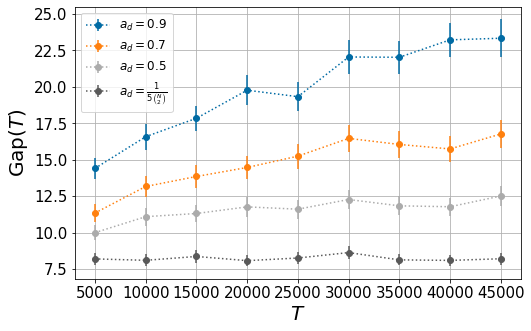
(a)

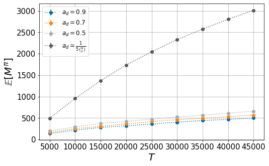
(b)

Figure 10: Dependence of system balancedness, number of flexes on the flex constant under the dynamic policy.

Appendix C Application to Parcel Delivery: A Case Study

C.1 Additional Details on Inputs

Derivation of transportation cost $c^{r}$.

This is based on an average truck speed of 15.75 km per hour in the dataset, a cost of gas of $0.956 per liter [Pri], and an average gas consumption of $0.35-0.5$ liters per km [Bud22].

Derivation of overtime cost $c^{o}$.

This is based on an average hourly wage of $22-$28 per hour for California truck drivers [Ind23], with an overtime payment multiplier of 1.5 [Doy22].

C.2 Creating a Default Truck Assignment via Clustering

To infer packages’ default truck assignments, we propose a heuristic for the capacitated $K$-means problem. Namely, we first apply a standard $K$-means clustering technique, letting $K=N$, to partition the packages into $N$ different zones. Given the geographic centers of each of these $N$ zones, we then re-assign packages to the zones, minimizing the total distance between packages and the center of their assigned zones, subject to a capacity constraint.

To formalize this latter step, we introduce some notation. Let $L$ denote the total number of packages that need to be clustered, and $z_{ij}$ be the binary variable that captures whether package $j$ is assigned to zone $i,\forall i=1,...,N,j=1,...,L$. We impose that each zone should be roughly balanced, i.e., the number of packages assigned to each zone should be within $\epsilon$ of the average number of packages per truck $L/N$, taking $\epsilon=200$. Finally, let $c_{ij}$ be the distance between package $j$ and the center of zone $i$. Then, the re-assignment problem is given in (73).

$$\begin{split}\min&\sum_{i=1}^{N}\sum_{j=1}^{L}c_{ij}z_{ij}\\ \text{s.t. }&L/N-\epsilon\leq\sum_{j=1}^{L}z_{ij}\leq L/N+\epsilon,\forall i\\ &\sum_{i=1}^{N}z_{ij}=1,\forall j,\quad z_{ij}\in\{0,1\},\forall i,j.\end{split}$$ (73)

C.3 Comparison of Historical and Synthetic Datasets

Throughout the period of interest, 448 historical routes originated from DLA8, serving a total of $L=57,359$ packages. Though routes took less than 7.50 hours on average to complete, approximately 30% of them exceeded 8 hours. Assuming inputs of $c^{o}=\$38$ per hour and $c^{r}=\$6.3$ per hour, this resulted in average overtime and transportation costs of $\$4.79$ and $\$14.24$, respectively, per route. Our re-sampled distribution of route completion times is roughly consistent with that of the historical data: the average completion time per route for our synthetic dataset is 7.42 hours, with 28.5% of routes exceeding 8 hours. Since the re-sampled data typically spans a larger geographic area per day, a larger fraction of the time is spent on travel, with average overtime and transportation costs of $\$6.14$ and $\$25.12$, respectively, per route. Despite the re-sampled data leading to both higher overtime and transportation costs, it preserves the feature that both overtime and transportation costs are important components of the cost objective, and the split of the costs among overtime and transportation is comparable with that of the historical dataset. Table 7 includes additional summary statistics on historical and synthetic routes.

	Route completion time (hours)				Unloading-to-travel time ratio				Number of stops per route
	Mean	$Q_{1}$	Median	$Q_{3}$	Mean	$Q_{1}$	Median	$Q_{3}$	Mean	$Q_{1}$	Median	$Q_{3}$
Historical	$7.50$	$6.91$	$7.58$	$8.10$	$2.62$	$1.73$	$2.40$	$3.34$	$129.03$	$106.75$	$131.00$	$152.00$
Bootstrapped	$7.42$	$6.77$	$7.44$	$8.10$	$0.92$	$0.62$	$0.84$	$1.15$	$83.33$	$76.00$	$83.00$	$90.00$

Table 7: Route Statistics for DLA8

C.4 Cost Minimization Heuristic

In this section, we outline a cost minimization heuristic as a point of comparison to the balancing policies examined in Section 4.3. Recall that in Algorithm 2 a flex is exerted if the difference in route completion times between two trucks exceeds a dynamic threshold that scales with $T-t.$ Here we follow a similar idea but pivot our approach slightly by opting to flex when the projected cost difference between flexing and not flexing surpasses the dynamic threshold.

Specifically, when determining whether to flex from $P(t)$ to truck $i,$ we use $y_{j}^{r}(t)$ and $y_{j}(t)$ to denote the predicted travel and route completion times of truck $j$ without flexing, and $\hat{y}_{j}^{r}(t)$ and $\hat{y}_{j}(t)$ to denote those times if the flex is implemented. Then, the expected cost difference between not flexing and flexing can be approximated by:

$$\begin{split}&c^{o}\left(\mathbb{E}\left[\left(y_{P(t)}(T+1)-8\right)^{+}\right]+\mathbb{E}\left[\left(y_{i}(T+1)-8\right)^{+}\right]-\mathbb{E}\left[\left(\hat{y}_{P(t)}(T+1)-8\right)^{+}\right]-\mathbb{E}\left[\left(\hat{y}_{i}(T+1)-8\right)^{+}\right]\right)\\ &\qquad+c^{r}\left(\mathbb{E}\left[y_{P(t)}^{r}(T+1)\right]+\mathbb{E}\left[y_{i}^{r}(T+1)\right]-\mathbb{E}\left[\hat{y}_{P(t)}^{r}(T+1)\right]-\mathbb{E}\left[\hat{y}_{i}^{r}(T+1)\right]\right).\end{split}$$ (74)

We trigger a flex into a truck that maximizes (74) if and only if this difference is at least $\frac{T-t}{M_{2}}.$ To find the distribution of $y_{j}(T+1)$ for a truck $j$ considered in (74), we assume future packages arriving in zone $j$ are drawn from a binomial distribution with $T-t$ trials and success probability $p_{j}$, with $p_{j}$ being bootstrapped from historical data. Let $N_{j}(T-t)$ denote the number of such packages. Then, we approximate $y_{j}(T+1)$ as:

$$y_{j}(T+1)=y_{j}(t)+\left(\texttt{INC}_{j}+\texttt{SER}_{j}\right)\cdot N_{j}(T-t)+\mathbbm{1}_{j=P(t)}\cdot\left(\texttt{INC}(S_{P(t)},t)+\texttt{SER}(t)\right),$$

where $\texttt{INC}_{j}$ and $\texttt{SER}_{j}$ are bootstrapped estimates of the incremental travel and unloading times for the no-flex policy. Distributions of $y_{j}^{r}(T+1),\hat{y}_{j}(T+1)$ and $\hat{y}_{j}^{r}(T+1)$ can be derived in a similar manner.

The performance of this heuristic is presented in Fig. 11 and Table 8. While this cost minimization heuristic effectively reduces average overtime, as shown by area II in Fig. 11, it does not provide additional cost savings relative to the Patient-Dynamic policy, which, recall, achieves cost savings of up to 7% relative to the no-flex policy. A closer comparison of the cost minimization heuristic and the Patient-Dynamic policy in Fig. 12 reveals that the former leads to a reduction in travel time but an increase in overtime. This is likely because the heuristic strongly depends on relatively accurate predictions of future travel and route completion times, which is challenging, despite access to bootstrapped data with i.i.d. package arrivals. The Patient-Dynamic policy, on the other hand, achieves strong performance with the need for significantly less information (namely, only approximations to the incremental travel time a package creates for a route).

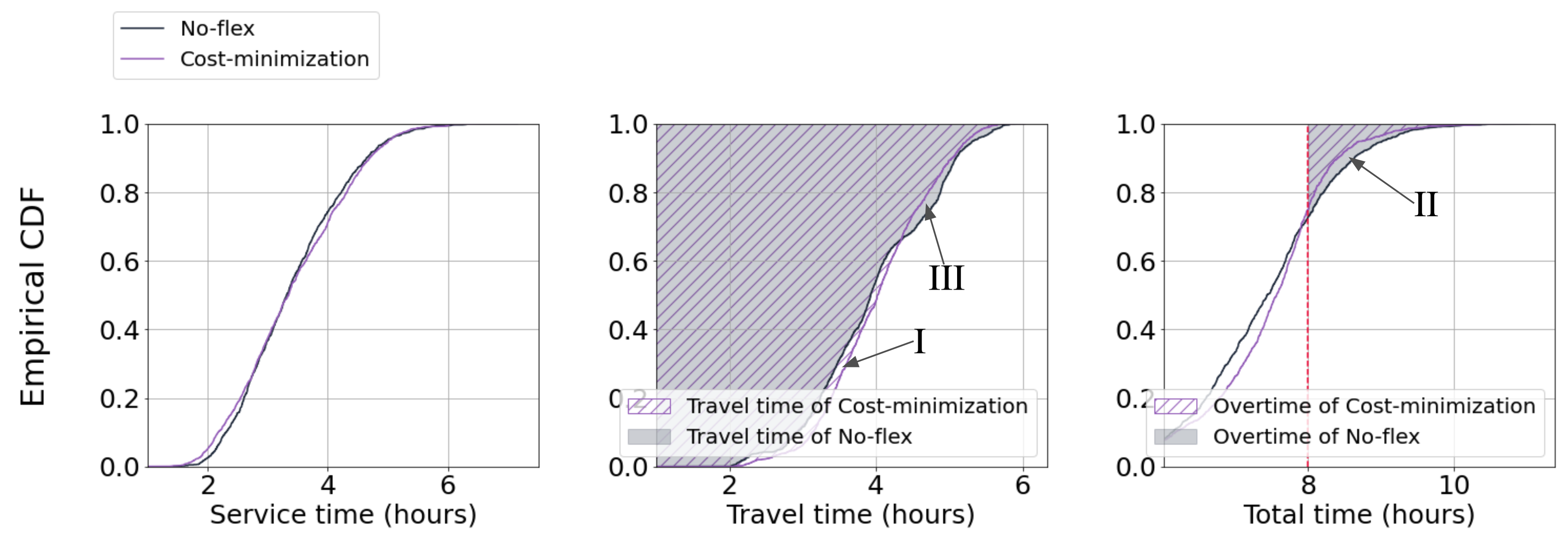
Figure 11: Unloading, travel, and total route completion times under the cost minimization heuristic and the no-flex policy. Area I captures the additional travel time required by the cost minimization heuristic. Areas II and III respectively capture the reduction in overtime and travel time of the cost minimization heuristic relative to the no-flex policy.

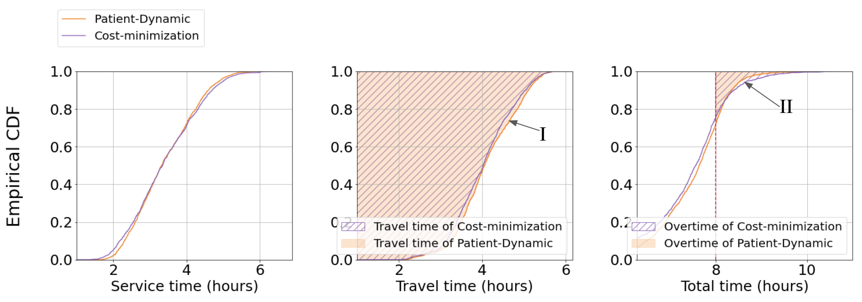
Figure 12: Unloading, travel, and total route completion times under the cost minimization heuristic and the Patient-Dynamic policy. Area I captures the reduction in travel time and Area II captures the additional overtime required by the cost minimization heuristic relative to the Patient-Dynamic policy.

Parameters			Costs
Travel cost	Overtime cost	Overtime threshold	No-flex	Cost-minimization	Relative difference
5.00	38.00	8.00	627.69	591.13	-5.82%
5.50	38.00	8.00	675.56	639.53	-5.33%
6.00	38.00	8.00	723.43	687.92	-4.91%
6.50	38.00	8.00	771.29	736.32	-4.53%
7.00	38.00	8.00	819.16	784.72	-4.20%
7.50	38.00	8.00	867.03	833.11	-3.91%
6.30	32.00	8.00	728.62	700.04	-3.92%
6.30	34.00	8.00	736.46	705.68	-4.18%
6.30	36.00	8.00	744.30	711.32	-4.43%
6.30	38.00	8.00	752.15	716.96	-4.68%
6.30	40.00	8.00	759.99	722.60	-4.92%
6.30	42.00	8.00	767.83	728.24	-5.16%
6.30	38.00	7.50	921.27	896.88	-2.65%
6.30	38.00	8.00	752.15	716.96	-4.68%
6.30	38.00	8.50	664.84	649.40	-2.32%
6.30	38.00	9.00	625.95	625.02	-0.15%
6.30	38.00	9.50	610.89	615.26	1.18%

Table 8: Sensitivity analyses for the costs of no-flex and cost-minimization policies

C.5 Additional Experiments

We further demonstrate the effectiveness of the Patient-Dynamic policy by applying it to historical data at two additional stations, DLA9 and DBO3. We observe a comparable degree of success in cost reduction at these stations, relative to the no-flex policy. As illustrated in Fig. 13, the application of the Patient-Dynamic policy effectively curtails overtime. Additionally, Table 9 reveals an average cost reduction of up to 5% for DLA9 and 6% for DBO3, further affirming the efficacy of the Patient-Dynamic policy.

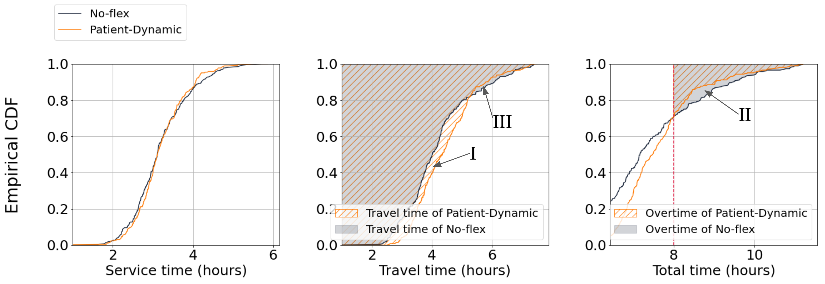
(a)

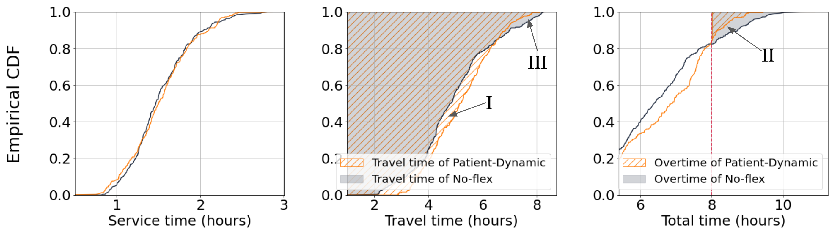
(b)

Figure 13: Unloading, travel, and total route completion times for DLA9 and DBO3. Area I captures the additional travel time required by the Patient-Dynamic policy. Areas II and III respectively capture the reduction in overtime and travel time of the Patient-Dynamic policy relative to the no-flex policy.

Parameters			Cost Reduction
Travel cost	Overtime cost	Overtime threshold	DLA8	DLA9	DBO3
5.00	38.00	8.00	7.18%	5.84%	6.39%
5.50	38.00	8.00	6.45%	5.18%	5.52%
6.00	38.00	8.00	5.81%	4.60%	4.77%
6.50	38.00	8.00	5.25%	4.08%	4.12%
7.00	38.00	8.00	4.76%	3.61%	3.55%
7.50	38.00	8.00	4.32%	3.18%	3.04%
6.30	32.00	8.00	4.33%	3.20%	3.06%
6.30	34.00	8.00	4.72%	3.57%	3.50%
6.30	36.00	8.00	5.10%	3.93%	3.94%
6.30	38.00	8.00	5.47%	4.28%	4.37%
6.30	40.00	8.00	5.83%	4.62%	4.79%
6.30	42.00	8.00	6.18%	4.94%	5.21%
6.30	38.00	7.50	1.16%	1.77%	2.20%
6.30	38.00	8.00	5.47%	4.28%	4.37%
6.30	38.00	8.50	3.18%	2.90%	2.11%
6.30	38.00	9.00	-0.57%	-0.29%	-1.45%
6.30	38.00	9.50	-2.26%	-2.52%	-3.84%

Table 9: Sensitivity analyses for the costs of no-flex and cost-minimization policies

C.6 On the uncapacitated assumption

We conclude this section by verifying the limitations of the uncapacitated assumption. In our experiments, a truck under the no-flex policy visits at most $117$ stops per day, with a 90th percentile of 98 stops; under Algorithm 2, a truck visits at most $117$ stops per day and has a 90th percentile of $99$ stops per day. Given the similarities in these values, we can reasonably deduce that if a truck does not encounter capacity constraints in the absence of balancing measures, it should also not face such constraints when implementing balancing policies.

References

- [ABKU94] Yossi Azar, Andrei Z Broder, Anna R Karlin, and Eli Upfal. Balanced allocations. In Proceedings of the twenty-sixth annual ACM symposium on theory of computing, pages 593–602, 1994.
- [Bud22] Budget Direct. Average Fuel Consumption in Australia. Online, 2022.
- [CD13a] John Gunnar Carlsson and Erick Delage. Robust partitioning for stochastic multivehicle routing. Operations research, 61(3):727–744, 2013.
- [CD13b] John Gunnar Carlsson and Raghuveer Devulapalli. Dividing a territory among several facilities. INFORMS Journal on Computing, 25(4):730–742, 2013.
- [CHH22] William Cook, Stephan Held, and Keld Helsgaun. Constrained local search for last-mile routing. Transportation Science, 2022.
- [CL06] Fan Chung and Linyuan Lu. Concentration inequalities and martingale inequalities: a survey. Internet Mathematics, 3(1):79–127, 2006.
- [CLSY21] John Gunnar Carlsson, Sheng Liu, Nooshin Salari, and Han Yu. Provably good region partitioning for on-time last-mile delivery. Rotman School of Management Working Paper, (3915544), 2021.
- [Doy22] Alison Doyle. How overtime pay is calculated. Online, 2022.
- [DP09] Devdatt P Dubhashi and Alessandro Panconesi. Concentration of measure for the analysis of randomized algorithms. Cambridge University Press, 2009.
- [DWWY21] Levi DeValve, Yehua Wei, Di Wu, and Rong Yuan. Understanding the value of fulfillment flexibility in an online retailing environment. Manufacturing & Service Operations Management, 2021.
- [EH21] Adam N Elmachtoub and Michael L Hamilton. The power of opaque products in pricing. Management Science, 2021.
- [Ell15] Glenn A Elliott. Real-time scheduling for GPUs with applications in advanced automotive systems. PhD thesis, The University of North Carolina at Chapel Hill, 2015.
- [ELZ21] Adam N Elmachtoub, Xiao Lei, and Yeqing Zhou. The value of consumer flexibility in scheduled service systems, 2021.
- [EWZ15] Adam N Elmachtoub, Yehua Wei, and Yeqing Zhou. Retailing with opaque products. Available at SSRN 2659211, 2015.
- [EYZ19] Adam N Elmachtoub, David Yao, and Yeqing Zhou. The value of flexibility from opaque selling. Available at SSRN 3483872, 2019.
- [Fel] William Feller. An introduction to probability theory and its applications. 1957.
- [FvR21] Daniel Freund and Garrett van Ryzin. Pricing fast and slow: Limitations of dynamic pricing mechanisms in ride-hailing. Available at SSRN 3931844, 2021.
- [FX08] Scott Fay and Jinhong Xie. Probabilistic goods: A creative way of selling products and services. Marketing Science, 27(4):674–690, 2008.
- [GP04] Guillermo Gallego and Robert Phillips. Revenue management of flexible products. Manufacturing & Service Operations Management, 6(4):321–337, 2004.
- [GRW+08] Bruce L Golden, Subramanian Raghavan, Edward A Wasil, et al. The vehicle routing problem: latest advances and new challenges, volume 43. Springer, 2008.
- [GS20] Geoffrey Grimmett and David Stirzaker. Probability and random processes. Oxford university press, 2020.
- [GY21] Negin Golrezaei and Evan Yao. Online resource allocation with time-flexible customers. arXiv preprint arXiv:2108.03517, 2021.
- [Har90] Ford W Harris. How many parts to make at once. Operations Research, 38(6):947–950, 1990.
- [HHL07] Dag Haugland, Sin C Ho, and Gilbert Laporte. Designing delivery districts for the vehicle routing problem with stochastic demands. European Journal of Operational Research, 180(3):997–1010, 2007.
- [Ind23] Indeed. Truck driver salaries in california. Online, 2023.
- [JG95] William C Jordan and Stephen C Graves. Principles on the benefits of manufacturing process flexibility. Management science, 41(4):577–594, 1995.
- [Jia07] Yabing Jiang. Price discrimination with opaque products. Journal of Revenue and Pricing Management, 6(2):118–134, 2007.
- [JNV09] Kinshuk Jerath, Serguei Netessine, and Senthil K Veeraraghavan. Selling to strategic customers: Opaque selling strategies. In Consumer-driven demand and operations management models, pages 253–300. Springer, 2009.
- [JW08] Patrick Jaillet and Michael R Wagner. Online vehicle routing problems: A survey. The Vehicle Routing Problem: Latest Advances and New Challenges, pages 221–237, 2008.
- [MAP+22] Daniel Merchan, Jatin Arora, Julian Pachon, Karthik Konduri, Matthias Winkenbach, Steven Parks, and Joseph Noszek. 2021 Amazon Last Mile Routing Research Challenge: Data set. Transportation Science, 2022.
- [Mit96] M Mitzenmacher. The power of two choices in randomized load balancing. PhD thesis, University of California at Berkeley, 1996.
- [Mit01] Michael Mitzenmacher. The power of two choices in randomized load balancing. IEEE Transactions on Parallel and Distributed Systems, 12(10):1094–1104, 2001.
- [MS22] Andrea Mor and Maria Grazia Speranza. Vehicle routing problems over time: a survey. Annals of Operations Research, 314(1):255–275, 2022.
- [Pri] Global Petrol Prices. Gasoline prices in the usa. https://www.globalpetrolprices.com/USA/gasoline_prices/. [Online; accessed 20-February-2023].
- [PTW10] Yuval Peres, Kunal Talwar, and Udi Wieder. The (1+ )-choice process and weighted balls-into-bins. In Proceedings of the twenty-first annual ACM-SIAM symposium on Discrete Algorithms, pages 1613–1619. SIAM, 2010.
- [RMS01] Andrea W Richa, M Mitzenmacher, and R Sitaraman. The power of two random choices: A survey of techniques and results. Combinatorial Optimization, 9:255–304, 2001.
- [RS98] Martin Raab and Angelika Steger. “balls into bins”—a simple and tight analysis. In International Workshop on Randomization and Approximation Techniques in Computer Science, pages 159–170. Springer, 1998.
- [RZ23] S Raghavan and Rui Zhang. The driver-aide problem: Coordinated logistics for last-mile delivery. 2023.
- [TV14] Paolo Toth and Daniele Vigo. Vehicle routing: problems, methods, and applications. SIAM, 2014.
- [TX13] John N Tsitsiklis and Kuang Xu. On the power of (even a little) resource pooling. Stochastic Systems, 2(1):1–66, 2013.
- [TX17] John N Tsitsiklis and Kuang Xu. Flexible queueing architectures. Operations Research, 65(5):1398–1413, 2017.
- [WWZ21] Shixin Wang, Xuan Wang, and Jiawei Zhang. A review of flexible processes and operations. Production and Operations Management, 30(6):1804–1824, 2021.
- [XC14] Yongbo Xiao and Jian Chen. Evaluating the potential effects from probabilistic selling of similar products. Naval Research Logistics (NRL), 61(8):604–620, 2014.
- [ZT22] Wenchang Zhu and Huseyin Topaloglu. Performance guarantees for network revenue management with flexible products. 2022.