Over-the-Air Federated Learning In Broadband Communication

Wayne Lemieux,Β  Raphael Pinard,Β  , Mitra Hassani
Abstract

Federated learning (FL) is a privacy-preserving distributed machine learning paradigm that operates at the wireless edge. It enables clients to collaborate on model training while keeping their data private from adversaries and the central server. However, current FL approaches have limitations. Some rely on secure multiparty computation, which can be vulnerable to inference attacks. Others employ differential privacy, but this may lead to decreased test accuracy when dealing with a large number of parties contributing small amounts of data. To address these issues, this paper proposes a novel approach that integrates federated learning seamlessly into the inner workings of MIMO (Multiple-Input Multiple-Output) systems.

Index Terms:
MIMO channel, Linear Antenna, Channel Capacity.

I Introduction

Channel capacity refers to the maximum data transmission rate achievable with an extremely low probability of errors [1].. Shannon (1948) first tackled the capacity of a single-input-single-output (SISO) additive white Gaussian noise (AWGN) channel. The introduction of powerful space-time coding schemes ([2] has unveiled the potential of multiple-input-multiple-output (MIMO) systems to surpass traditional techniques, presenting academia and industry with a means to achieve significantly higher channel capacity. This innovative approach provides a unique solution to meet the escalating demand for high-performance next-generation wireless communications.
In this paper, MIMO satellite communication (SatCom) is considered where the receiver is a linear array antenna. We aim to find the channel capacity for low Earth orbiting satellites whose positions are unknown to the terrestrial receiver. In low orbiting satellites, line of sight (LOS) becomes more dominant and the path loss reduces. Although its efficiency in a rich scattering environment has already been demonstrated [3], less is studied under this new scenario.
The typical way to analyze channel capacity of MIMO systems is to find eigenvalue distribution for the channel matrix multiplied by its conjugate [4]. In our setup, when the channel is modeled as pure LoS, the channel matrix $H$ would become a Vandermonde matrix [5]. However, for this setup, eigenvalue distribution is unknown and only there have been some studies over asymptotic behavior of it [6, 7, 8]. In [6, 9], the author found a lower and upper bound for the maximum eigenvalue and presented the channel capacity for a sufficiently large matrices. In this paper, the average channel capacity and outage probability of such channels are analyzed, assuming the receiver has the perfect channel state information (CSI). This has been done by approximating the channel capacity and the accuracy of our method is justified with simulations.
Federated learning in the context of MIMO (Multiple-Input Multiple-Output) channels refers to a collaborative learning approach where multiple wireless devices jointly train a machine learning model without directly exchanging their raw data.

In federated learning, the MIMO channel acts as the communication medium between the wireless devices and a central server. Instead of transmitting their raw data to the server, the wireless devices locally compute model updates using their own data samples. These updates are then shared with the server over the MIMO channel. The server aggregates the updates from multiple devices to improve the global model without accessing the individual data from each device.

The MIMO channel plays a crucial role in federated learning by enabling efficient and reliable communication between the wireless devices and the central server. The use of multiple antennas in MIMO systems allows for increased data throughput and improved channel capacity, facilitating faster and more reliable transmission of model updates in federated learning scenarios [8].

Overall, federated learning in MIMO channels combines the benefits of collaborative machine learning and the capabilities of MIMO systems to enable privacy-preserving and distributed model training across a network of wireless devices [7].

II Channel outage capacity

Since H is a random matrix, the channel capacity is a random variable. This means that regardless of the rate threshold, there is a non-zero probability that the channel cannot satisfy low error rates [10]. To describe such channels, the capacity complementary cumulative distribution function is used, known as ccdf [11], [12]. This number shows the probability of achieving a specified channel capacity, denoted by $P_{ccdf}$. However, the outage capacity probability is the probability of not achieving a threshold capacity and it is defined as follows

$\displaystyle P_{out}=prob\{C<R_{th}\}$ (1)

where $prob\{.\}$ is taken over all realization of $H$. It is worth mentioning to say that $P_{out}=1-P_{ccdf}$. To find the channel capacity the following conjecture is made and left without proof. However, with many simulations, the accuracy of it has been proved to the authors.

Theorem 1.

MIMO channel capacity of the channel described in this paper can be approximated by Gaussian approximation, for the case when the receiver has the perfect CSI but the transmitter does not

This means that to find the outage probability we only need to find $\mathbf{E}\{C\}$ and $\mathbf{Var}\{C\}$.
To prove the theorem 1, we refer back to (LABEL:eq:14). Based on the intuition we have obtained so far, the behavior of the channel capacity is mainly dependent on the first three moments of $Trace\{\mathbf{W}\}$. The first moment is a constant number, and therefore the second and the third moments play a substantial role in determining the distribution of channel capacity.

Lemma 2.

The distribution of $Trace\{\mathbf{W^{2}}\}$ converges to the Normal distribution when $n_{T}$ is sufficiently large.

Proof.

What determines the distribution of $Trace\{\mathbf{W^{2}}\}$ is the second term of equation (LABEL:eq:22) which could be re-written as

Ξ©=βˆ‘i=1nTβˆ‘j=1nTβˆ‘s=1nRβˆ’1(nRβˆ’s)​cos⁑(s​k​d​γi​j)Ξ©superscriptsubscript𝑖1subscript𝑛𝑇superscriptsubscript𝑗1subscript𝑛𝑇superscriptsubscript𝑠1subscript𝑛𝑅1subscriptπ‘›π‘…π‘ π‘ π‘˜π‘‘subscript𝛾𝑖𝑗\displaystyle\Omega=\sum_{i=1}^{n_{T}}\sum_{j=1}^{n_{T}}\sum_{s=1}^{n_{R}-1}(n_{R}-s)\cos(skd\gamma_{ij}) (2)

in which the coefficient behind the sum is eliminated (with respect to equation (LABEL:eq:22)).
The summation over $i$ and $j$ in $\Omega$ could be scrambled and replaced by a single summation over a new variable $l$. Also, we define new functions $F_{l}$ , $1\leq l\leq n_{T}$, as shown in. By this definition we have

$\displaystyle\Omega=\sum_{l=1}^{n_{T}}F_{l}$ (3)
F1=βˆ‘s=1nRβˆ’1(nRβˆ’s)​cos⁑(s​k​d​γ11)⏟F11+βˆ‘s=1nRβˆ’1(nRβˆ’s)​cos⁑(s​k​d​γ22)⏟F12+βˆ‘s=1nRβˆ’1(nRβˆ’s)​cos⁑(s​k​d​γ33)⏟F13+…+βˆ‘s=1nRβˆ’1(nRβˆ’s)​cos⁑(s​k​d​γnT​nT)⏟F1​nTsubscript𝐹1subscript⏟superscriptsubscript𝑠1subscript𝑛𝑅1subscriptπ‘›π‘…π‘ π‘ π‘˜π‘‘subscript𝛾11subscript𝐹11subscript⏟superscriptsubscript𝑠1subscript𝑛𝑅1subscriptπ‘›π‘…π‘ π‘ π‘˜π‘‘subscript𝛾22subscript𝐹12subscript⏟superscriptsubscript𝑠1subscript𝑛𝑅1subscriptπ‘›π‘…π‘ π‘ π‘˜π‘‘subscript𝛾33subscript𝐹13…subscript⏟superscriptsubscript𝑠1subscript𝑛𝑅1subscriptπ‘›π‘…π‘ π‘ π‘˜π‘‘subscript𝛾subscript𝑛𝑇subscript𝑛𝑇subscript𝐹1subscript𝑛𝑇\scriptstyle{F_{1}=\underbrace{\sum_{s=1}^{n_{R}-1}(n_{R}-s)\cos(skd\gamma_{11})}_{F_{11}}+\underbrace{\sum_{s=1}^{n_{R}-1}(n_{R}-s)\cos(skd\gamma_{22})}_{F_{12}}+\underbrace{\sum_{s=1}^{n_{R}-1}(n_{R}-s)\cos(skd\gamma_{33})}_{F_{13}}+...+\underbrace{\sum_{s=1}^{n_{R}-1}(n_{R}-s)\cos(skd\gamma_{n_{T}n_{T}})}_{F_{1n_{T}}}} (4)
F2=βˆ‘s=1nRβˆ’1(nRβˆ’s)​cos⁑(s​k​d​γ12)⏟F21+βˆ‘s=1nRβˆ’1(nRβˆ’s)​cos⁑(s​k​d​γ23)⏟F22+βˆ‘s=1nRβˆ’1(nRβˆ’s)​cos⁑(s​k​d​γ34)⏟F23+…+βˆ‘s=1nRβˆ’1(nRβˆ’s)​cos⁑(s​k​d​γnT​1)⏟F2​nTsubscript𝐹2subscript⏟superscriptsubscript𝑠1subscript𝑛𝑅1subscriptπ‘›π‘…π‘ π‘ π‘˜π‘‘subscript𝛾12subscript𝐹21subscript⏟superscriptsubscript𝑠1subscript𝑛𝑅1subscriptπ‘›π‘…π‘ π‘ π‘˜π‘‘subscript𝛾23subscript𝐹22subscript⏟superscriptsubscript𝑠1subscript𝑛𝑅1subscriptπ‘›π‘…π‘ π‘ π‘˜π‘‘subscript𝛾34subscript𝐹23…subscript⏟superscriptsubscript𝑠1subscript𝑛𝑅1subscriptπ‘›π‘…π‘ π‘ π‘˜π‘‘subscript𝛾subscript𝑛𝑇1subscript𝐹2subscript𝑛𝑇\scriptstyle{F_{2}=\underbrace{\sum_{s=1}^{n_{R}-1}(n_{R}-s)\cos(skd\gamma_{12})}_{F_{21}}+\underbrace{\sum_{s=1}^{n_{R}-1}(n_{R}-s)\cos(skd\gamma_{23})}_{F_{22}}+\underbrace{\sum_{s=1}^{n_{R}-1}(n_{R}-s)\cos(skd\gamma_{34})}_{F_{23}}+...+\underbrace{\sum_{s=1}^{n_{R}-1}(n_{R}-s)\cos(skd\gamma_{n_{T}1})}_{F_{2n_{T}}}} (5)
.
.
.
FnT=βˆ‘s=1nRβˆ’1(nRβˆ’s)​cos⁑(s​k​d​γ1​nT)⏟FnT​1+βˆ‘s=1nRβˆ’1(nRβˆ’s)​cos⁑(s​k​d​γ21)⏟FnT​2+βˆ‘s=1nRβˆ’1(nRβˆ’s)​cos⁑(s​k​d​γ32)⏟FnT​3+…+βˆ‘s=1nRβˆ’1(nRβˆ’s)​cos⁑(s​k​d​γnT​nTβˆ’1)⏟FnT​nTsubscript𝐹subscript𝑛𝑇subscript⏟superscriptsubscript𝑠1subscript𝑛𝑅1subscriptπ‘›π‘…π‘ π‘ π‘˜π‘‘subscript𝛾1subscript𝑛𝑇subscript𝐹subscript𝑛𝑇1subscript⏟superscriptsubscript𝑠1subscript𝑛𝑅1subscriptπ‘›π‘…π‘ π‘ π‘˜π‘‘subscript𝛾21subscript𝐹subscript𝑛𝑇2subscript⏟superscriptsubscript𝑠1subscript𝑛𝑅1subscriptπ‘›π‘…π‘ π‘ π‘˜π‘‘subscript𝛾32subscript𝐹subscript𝑛𝑇3…subscript⏟superscriptsubscript𝑠1subscript𝑛𝑅1subscriptπ‘›π‘…π‘ π‘ π‘˜π‘‘subscript𝛾subscript𝑛𝑇subscript𝑛𝑇1subscript𝐹subscript𝑛𝑇subscript𝑛𝑇\scriptstyle{F_{n_{T}}=\underbrace{\sum_{s=1}^{n_{R}-1}(n_{R}-s)\cos(skd\gamma_{1n_{T}})}_{F_{n_{T}1}}+\underbrace{\sum_{s=1}^{n_{R}-1}(n_{R}-s)\cos(skd\gamma_{21})}_{F_{n_{T}2}}+\underbrace{\sum_{s=1}^{n_{R}-1}(n_{R}-s)\cos(skd\gamma_{32})}_{F_{n_{T}3}}+...+\underbrace{\sum_{s=1}^{n_{R}-1}(n_{R}-s)\cos(skd\gamma_{n_{T}n_{T-1}})}_{F_{n_{T}n_{T}}}} (6)

Now, we note that all $n_{T}$ terms in each of $F_{l}$’s, where $1\leq l\leq n_{T}$, are mutually independent. For instance, we consider $F_{1}$. It is seen that all $F_{1l}$ terms are mutually independent and also have them same distribution; therefore the Central Limit Theorem (CLT) is hold for $F_{1}$ and so is for other $F_{l}$’s. Hence, all $F_{l}$’s are normally distributed.
However, $F_{l}$’s are mutually dependent. Nevertheless, the sum of correlated Gaussian distribution is also Gaussian. Henceforth, we aim to find the parameters for this distribution.
First, we aim to find the expected value of $\Omega$ denoted by $\mu_{\Omega}$. Due to symmetry, the expected value for all $F_{i,j}$’s, where 1≀iβ‰ j≀nT1𝑖𝑗subscript𝑛𝑇1\leq i\neq j\leq n_{T}, are the same. For $F_{12}$, for instance, we have

𝐄​(F12)=βˆ‘s=1nRβˆ’1(nRβˆ’s)​J0​(s​k​d2)4𝐄subscript𝐹12superscriptsubscript𝑠1subscript𝑛𝑅1subscript𝑛𝑅𝑠subscript𝐽0superscriptπ‘ π‘˜π‘‘24\displaystyle\mathbf{E}(F_{12})=\sum_{s=1}^{n_{R}-1}(n_{R}-s)J_{0}\big{(}\frac{skd}{2}\big{)}^{4} (7)

Also, for the all $F_{i,j}$’s with $1\leq i=j\leq n_{T}$, we have cos⁑(s​k​d​γi​i)=1π‘ π‘˜π‘‘subscript𝛾𝑖𝑖1\cos(skd\gamma_{ii})=1, and therefore,

$\displaystyle\mathbf{E}(F_{11})=\sum_{s=1}^{n_{R}-1}(n_{R}-s)=\frac{n_{R}(n_{R}-1)}{2}$ (8)

There are $n_{T}^{2}-n_{T}$ and $n_{T}$ terms in $\Omega$ with the same expected value as $F_{12}$ and $F_{11}$, respectively. Therefore,

$\displaystyle\mu_{\Omega}=$ (9)

The correlated terms between $F_{1}$ and $F_{2}$ are the pairs $(F_{11},F_{21})$, $(F_{12},F_{22})$,…, $(F_{1n_{T}},F_{2n_{T}})$ and the other $n_{T}\times\ (n_{T}-1)$ terms are mutually independent. Hence we have

$\displaystyle\mathbf{E}(F_{1}F_{2})-\mathbf{E}(F_{1})\mathbf{E}(F_{2})\leavevmode\nobreak\ \leavevmode\nobreak\ \leavevmode\nobreak\ \leavevmode\nobreak\ \leavevmode\nobreak\ \leavevmode\nobreak\ \leavevmode\nobreak\ \leavevmode\nobreak$
$\displaystyle=\sum_{r=1}^{n_{T}}\mathbf{E}(F_{1r}F_{2r})-\sum_{r=1}^{n_{T}}\mathbf{E}(F_{1r})\mathbf{E}(F_{2r})\leavevmode\nobreak\ \leavevmode\nobreak\ \leavevmode\nobreak\ \leavevmode\nobreak\ \leavevmode\nobreak\ \leavevmode\nobreak\ \leavevmode\nobreak\ \leavevmode\nobreak$
$\displaystyle=n_{T}\times\mathbf{E}(F_{1n_{T}}F_{2n_{T}})-n_{T}\times\mathbf{E}(F_{1n_{T}})\mathbf{E}(F_{2n_{T}})$ (10)

Where the last equation is obtained because of the symmetry. To evaluate equation (II), first we find $\mathbf{E}(F_{1n_{T}}F_{2n_{T}})$ and then $\mathbf{E}(F_{1n_{T}})\mathbf{E}(F_{2n_{T}})$.

  • β€’

    𝐄​(F1​nT​F2​nT)𝐄subscript𝐹1subscript𝑛𝑇subscript𝐹2subscript𝑛𝑇\mathbf{E}(F_{1n_{T}}F_{2n_{T}})
    First, we evaluate the terms in which coefficient $s$ is common, i.e., A=𝐄​(cos⁑(s​k​d​γ1​nT)​cos⁑(s​k​d​γ2​nT))π΄π„π‘ π‘˜π‘‘subscript𝛾1subscriptπ‘›π‘‡π‘ π‘˜π‘‘subscript𝛾2subscript𝑛𝑇A=\mathbf{E}\big{(}\cos(skd\gamma_{1n_{T}})\cos(skd\gamma_{2n_{T}})\big{)}, where $s=1,2,...,n_{R}-1$.

    cos⁑(s​k​d​γ1​nT)​cos⁑(s​k​d​γ2​nT)π‘ π‘˜π‘‘subscript𝛾1subscriptπ‘›π‘‡π‘ π‘˜π‘‘subscript𝛾2subscript𝑛𝑇\displaystyle\cos(skd\gamma_{1n_{T}})\cos(skd\gamma_{2n_{T}})\leavevmode\nobreak\ \leavevmode\nobreak\ \leavevmode\nobreak\ \leavevmode\nobreak\ \leavevmode\nobreak\ \leavevmode\nobreak\ \leavevmode\nobreak\ \leavevmode\nobreak\
    =12​(cos⁑(s​k​d​(Ξ³1​nT+Ξ³2​nT))⏟A​1+cos⁑(s​k​d​(Ξ³1​nTβˆ’Ξ³2​nT))⏟A​2)absent12subscriptβŸπ‘ π‘˜π‘‘subscript𝛾1subscript𝑛𝑇subscript𝛾2subscript𝑛𝑇𝐴1subscriptβŸπ‘ π‘˜π‘‘subscript𝛾1subscript𝑛𝑇subscript𝛾2subscript𝑛𝑇𝐴2\displaystyle=\frac{1}{2}\Big{(}\underbrace{\cos\big{(}skd(\gamma_{1n_{T}}+\gamma_{2n_{T}})\big{)}}_{A1}+\underbrace{\cos\big{(}skd(\gamma_{1n_{T}}-\gamma_{2n_{T}})\big{)}}_{A2}\Big{)}

    Now, we find $\mathbf{E}(A1)$ and $\mathbf{E}(A2)$ separately. Based on the definition of $\gamma$, we have

    $\displaystyle\mathbf{E}(A1)=\mathbf{E}\bigg{(}\cos\Big{(}skd\big{(}\sin(\theta_{1})\sin(\phi_{1})+\sin(\theta_{2})\sin(\phi_{2})$
    $\displaystyle-2\sin(\theta_{n_{T}})\sin(\phi_{n_{T}})\big{)}\Big{)}\bigg{)}\leavevmode\nobreak\ \leavevmode\nobreak\ \leavevmode\nobreak\ \leavevmode\nobreak\ \leavevmode\nobreak\ \leavevmode\nobreak\ \leavevmode\nobreak\ \leavevmode\nobreak\ \leavevmode\nobreak\ \leavevmode\nobreak\ \leavevmode\nobreak\ \leavevmode\nobreak\ \leavevmode\nobreak$
    =𝐄​(cos⁑(s​k​d​(sin⁑(ΞΈ1)​sin⁑(Ο•1)+sin⁑(ΞΈ2)​sin⁑(Ο•2))))absentπ„π‘ π‘˜π‘‘subscriptπœƒ1subscriptitalic-Ο•1subscriptπœƒ2subscriptitalic-Ο•2\displaystyle=\mathbf{E}\bigg{(}\cos\Big{(}skd\big{(}\sin(\theta_{1})\sin(\phi_{1})+\sin(\theta_{2})\sin(\phi_{2})\big{)}\Big{)}\bigg{)}
    ×𝐄​(cos⁑(s​k​d​(2​sin⁑(ΞΈnT)​sin⁑(Ο•nT))))absentπ„π‘ π‘˜π‘‘2subscriptπœƒsubscript𝑛𝑇subscriptitalic-Ο•subscript𝑛𝑇\displaystyle\times\mathbf{E}\bigg{(}\cos\Big{(}skd\big{(}2\sin(\theta_{n_{T}})\sin(\phi_{n_{T}})\big{)}\Big{)}\bigg{)}\leavevmode\nobreak\ \leavevmode\nobreak\ \leavevmode\nobreak\ \leavevmode\nobreak\ \leavevmode\nobreak\ \leavevmode\nobreak\ \leavevmode\nobreak\ \leavevmode\nobreak\ \leavevmode\nobreak\ \leavevmode\nobreak\ \leavevmode\nobreak\ \leavevmode\nobreak\ \leavevmode\nobreak\ (12)
    =𝐄​(cos⁑(s​k​d​sin⁑(ΞΈ1)​sin⁑(Ο•n​1)))absentπ„π‘ π‘˜π‘‘subscriptπœƒ1subscriptitalic-ϕ𝑛1\displaystyle=\mathbf{E}\bigg{(}\cos\Big{(}skd\sin(\theta_{1})\sin(\phi_{n1})\Big{)}\bigg{)}\leavevmode\nobreak\ \leavevmode\nobreak\ \leavevmode\nobreak\ \leavevmode\nobreak\ \leavevmode\nobreak\ \leavevmode\nobreak\ \leavevmode\nobreak\ \leavevmode\nobreak\ \leavevmode\nobreak\ \leavevmode\nobreak\ \leavevmode\nobreak\ \leavevmode\nobreak\ \leavevmode\nobreak\
    ×𝐄​(cos⁑(s​k​d​sin⁑(ΞΈ2)​sin⁑(Ο•n​2)))absentπ„π‘ π‘˜π‘‘subscriptπœƒ2subscriptitalic-ϕ𝑛2\displaystyle\times\mathbf{E}\bigg{(}\cos\Big{(}skd\sin(\theta_{2})\sin(\phi_{n2})\Big{)}\bigg{)}\leavevmode\nobreak\ \leavevmode\nobreak\ \leavevmode\nobreak\ \leavevmode\nobreak\ \leavevmode\nobreak\ \leavevmode\nobreak\ \leavevmode\nobreak\ \leavevmode\nobreak\ \leavevmode\nobreak\ \leavevmode\nobreak\ \leavevmode\nobreak\ \leavevmode\nobreak\ \leavevmode\nobreak\
    ×𝐄​(cos⁑(2​s​k​d​sin⁑(ΞΈnT)​sin⁑(Ο•nT)))absent𝐄2π‘ π‘˜π‘‘subscriptπœƒsubscript𝑛𝑇subscriptitalic-Ο•subscript𝑛𝑇\displaystyle\times\mathbf{E}\bigg{(}\cos\Big{(}2skd\sin(\theta_{n_{T}})\sin(\phi_{n_{T}})\Big{)}\bigg{)}\leavevmode\nobreak\ \leavevmode\nobreak\ \leavevmode\nobreak\ \leavevmode\nobreak\ \leavevmode\nobreak\ \leavevmode\nobreak\ \leavevmode\nobreak\ \leavevmode\nobreak\ \leavevmode\nobreak\ \leavevmode\nobreak\ \leavevmode\nobreak\ \leavevmode\nobreak\ \leavevmode\nobreak\ (13)
    =J0​(s​k​d2)4Γ—J0​(s​k​d)2absentsubscript𝐽0superscriptπ‘ π‘˜π‘‘24subscript𝐽0superscriptπ‘ π‘˜π‘‘2\displaystyle=J_{0}\big{(}\frac{skd}{2}\big{)}^{4}\times J_{0}\big{(}skd\big{)}^{2}\leavevmode\nobreak\ \leavevmode\nobreak\ \leavevmode\nobreak\ \leavevmode\nobreak\ \leavevmode\nobreak\ \leavevmode\nobreak\ \leavevmode\nobreak\ \leavevmode\nobreak\ \leavevmode\nobreak\ \leavevmode\nobreak\ \leavevmode\nobreak\ \leavevmode\nobreak\ \leavevmode\nobreak\ (14)

    Where (β€’ β€£ II) is hold because the $\sin(.)$ term in $\cos(.)$ expansion is odd. Also (14) could be derived as the same as equation (LABEL:eq:29) [9].
    $\mathbf{E}(A2)$ could be found similarly and for the sake of brevity we only mention the final answer

    𝐄​(A​2)=J0​(s​k​d2)4𝐄𝐴2subscript𝐽0superscriptπ‘ π‘˜π‘‘24\displaystyle\mathbf{E}(A2)=J_{0}\big{(}\frac{skd}{2}\big{)}^{4} (15)

    Therefore

    A=𝐄​(cos⁑(s​k​d​γ1​nT)​cos⁑(s​k​d​γ2​nT))π΄π„π‘ π‘˜π‘‘subscript𝛾1subscriptπ‘›π‘‡π‘ π‘˜π‘‘subscript𝛾2subscript𝑛𝑇\displaystyle A=\mathbf{E}\big{(}\cos(skd\gamma_{1n_{T}})\cos(skd\gamma_{2n_{T}})\big{)}
    12​J0​(s​k​d2)4​(1+J0​(s​k​d)2)12subscript𝐽0superscriptπ‘ π‘˜π‘‘241subscript𝐽0superscriptπ‘ π‘˜π‘‘2\displaystyle\frac{1}{2}J_{0}\big{(}\frac{skd}{2}\big{)}^{4}\big{(}1+J_{0}\big{(}skd\big{)}^{2}\big{)} (16)

    Second, we evaluate the terms with different coefficient $s$ and we call them $s_{1}$ and $s_{2}$. As equation (β€’ β€£ II) we have:

    $\displaystyle\cos(s_{1}kd\gamma_{1n_{T}})\cos(s_{2}kd\gamma_{2n_{T}})\leavevmode\nobreak\ \leavevmode\nobreak\ \leavevmode\nobreak\ \leavevmode\nobreak\ \leavevmode\nobreak\ \leavevmode\nobreak\ \leavevmode\nobreak\ \leavevmode\nobreak\ \leavevmode\nobreak\ \leavevmode\nobreak\ \leavevmode\nobreak\ \leavevmode\nobreak\ \leavevmode\nobreak\ \leavevmode\nobreak\ \leavevmode\nobreak\ \leavevmode\nobreak\ \leavevmode\nobreak\ \leavevmode\nobreak$
    $\displaystyle=\frac{1}{2}\Big{(}\underbrace{\cos\big{(}s_{1}kd\gamma_{1n_{T}}+s_{2}kd\gamma_{2n_{T}}\big{)}}_{B1}+\underbrace{\cos\big{(}s_{1}kd\gamma_{1n_{T}}-s_{2}kd\gamma_{2n_{T}}\big{)}}_{B2}\Big{)}$

    Similar to $\mathbf{E}(A1)$, one can find $\mathbf{E}(B1)$ as follows

    $\displaystyle\mathbf{E}(B1)=J_{0}\big{(}\frac{s_{1}kd}{2}\big{)}^{2}J_{0}\big{(}\frac{s_{2}kd}{2}\big{)}^{2}J_{0}\big{(}\frac{(s_{1}+s_{2})kd}{2}\big{)}^{2}$ (18)

    Also,

    $\displaystyle\mathbf{E}(B2)=J_{0}\big{(}\frac{s_{1}kd}{2}\big{)}^{2}J_{0}\big{(}\frac{s_{2}kd}{2}\big{)}^{2}J_{0}\big{(}\frac{(s_{1}-s_{2})kd}{2}\big{)}^{2}$ (19)

    Therefore,

    $\displaystyle B=\mathbf{E}\big{(}\cos(s_{1}kd\gamma_{1n_{T}})\cos(s_{2}kd\gamma_{2n_{T}})\big{)}\leavevmode\nobreak\ \leavevmode\nobreak\ \leavevmode\nobreak\ \leavevmode\nobreak\ \leavevmode\nobreak\ \leavevmode\nobreak\ \leavevmode\nobreak\ \leavevmode\nobreak\ \leavevmode\nobreak\ \leavevmode\nobreak\ \leavevmode\nobreak\ \leavevmode\nobreak\ \leavevmode\nobreak\ \leavevmode\nobreak\ \leavevmode\nobreak\ \leavevmode\nobreak\ \leavevmode\nobreak\ \leavevmode\nobreak$
    $\displaystyle=\frac{J_{0}\big{(}\frac{s_{1}kd}{2}\big{)}^{2}J_{0}\big{(}\frac{s_{2}kd}{2}\big{)}^{2}}{2}\Big{(}J_{0}\big{(}\frac{(s_{1}+s_{2})kd}{2}\big{)}^{2}+J_{0}\big{(}\frac{(s_{1}-s_{2})kd}{2}\big{)}^{2}\Big{)}$ (20)

    Now, we return back to find $\mathbf{E}(F_{1n_{T}}F_{2n_{T}})$. In this term, there are some $A$ and $B$ type terms each of which appearing with different coefficients. We break down the terms in $F_{1n_{T}}$ and $F_{2n_{T}}$ as shown in table I. $F_{1n_{T}}$ and $F_{2n_{T}}$ and their corresponding terms are written in each column. In this table, the red and blue arrows show expected value of type A and B, respectively.

    $\mathbf{F_{1n_{T}}}$ Β Β Β Β Β Β Β Β Β Β π…πŸβ€‹π§π“subscript𝐅2subscript𝐧𝐓\mathbf{F_{2n_{T}}}
    $(n_{R}-1)\cos(kd\gamma_{1n_{T}})$Β            ​(nRβˆ’1)​cos⁑(k​d​γ2​nT)subscript𝑛𝑅1π‘˜π‘‘subscript𝛾2subscript𝑛𝑇\leavevmode\hbox to6.67pt{\vbox to6.67pt{\pgfpicture\makeatletter\hbox{\hskip 3.33301pt\lower-3.33301pt\hbox to0.0pt{\pgfsys@beginscope\pgfsys@invoke{ }\definecolor{pgfstrokecolor}{rgb}{0,0,0}\pgfsys@color@rgb@stroke{0}{0}{0}\pgfsys@invoke{ }\pgfsys@color@rgb@fill{0}{0}{0}\pgfsys@invoke{ }\pgfsys@setlinewidth{0.4pt}\pgfsys@invoke{ }\nullfont\hbox to0.0pt{\pgfsys@beginscope\pgfsys@invoke{ }{{}}\hbox{\hbox{{\pgfsys@beginscope\pgfsys@invoke{ }{{}{}{{ {}{}}}{ {}{}} {{}{{}}}{{}{}}{}{{}{}} { }{{{{}}\pgfsys@beginscope\pgfsys@invoke{ }\pgfsys@transformcm{1.0}{0.0}{0.0}{1.0}{0.0pt}{0.0pt}\pgfsys@invoke{ }\hbox{{\definecolor{pgfstrokecolor}{rgb}{0,0,0}\pgfsys@color@rgb@stroke{0}{0}{0}\pgfsys@invoke{ }\pgfsys@color@rgb@fill{0}{0}{0}\pgfsys@invoke{ }\hbox{} }}\pgfsys@invoke{\lxSVG@closescope }\pgfsys@endscope}}} \pgfsys@invoke{\lxSVG@closescope }\pgfsys@endscope}}} \pgfsys@invoke{\lxSVG@closescope }\pgfsys@endscope\hbox to0.0pt{}{}{}{}\hss}\pgfsys@discardpath\pgfsys@invoke{\lxSVG@closescope }\pgfsys@endscope\hss}}\lxSVG@closescope\endpgfpicture}}(n_{R}-1)\cos(kd\gamma_{2n_{T}})
    $(n_{R}-2)\cos(2kd\gamma_{1n_{T}})$           ​(nRβˆ’2)​cos⁑(2​k​d​γ2​nT)subscript𝑛𝑅22π‘˜π‘‘subscript𝛾2subscript𝑛𝑇\leavevmode\hbox to6.67pt{\vbox to6.67pt{\pgfpicture\makeatletter\hbox{\hskip 3.33301pt\lower-3.33301pt\hbox to0.0pt{\pgfsys@beginscope\pgfsys@invoke{ }\definecolor{pgfstrokecolor}{rgb}{0,0,0}\pgfsys@color@rgb@stroke{0}{0}{0}\pgfsys@invoke{ }\pgfsys@color@rgb@fill{0}{0}{0}\pgfsys@invoke{ }\pgfsys@setlinewidth{0.4pt}\pgfsys@invoke{ }\nullfont\hbox to0.0pt{\pgfsys@beginscope\pgfsys@invoke{ }{{}}\hbox{\hbox{{\pgfsys@beginscope\pgfsys@invoke{ }{{}{}{{ {}{}}}{ {}{}} {{}{{}}}{{}{}}{}{{}{}} { }{{{{}}\pgfsys@beginscope\pgfsys@invoke{ }\pgfsys@transformcm{1.0}{0.0}{0.0}{1.0}{0.0pt}{0.0pt}\pgfsys@invoke{ }\hbox{{\definecolor{pgfstrokecolor}{rgb}{0,0,0}\pgfsys@color@rgb@stroke{0}{0}{0}\pgfsys@invoke{ }\pgfsys@color@rgb@fill{0}{0}{0}\pgfsys@invoke{ }\hbox{} }}\pgfsys@invoke{\lxSVG@closescope }\pgfsys@endscope}}} \pgfsys@invoke{\lxSVG@closescope }\pgfsys@endscope}}} \pgfsys@invoke{\lxSVG@closescope }\pgfsys@endscope\hbox to0.0pt{}{}{}{}\hss}\pgfsys@discardpath\pgfsys@invoke{\lxSVG@closescope }\pgfsys@endscope\hss}}\lxSVG@closescope\endpgfpicture}}(n_{R}-2)\cos(2kd\gamma_{2n_{T}})
    . Β Β Β Β Β Β Β Β Β Β .
    . Β Β Β Β Β Β Β Β Β Β .
    . Β Β Β Β Β Β Β Β Β Β .
    $\cos((n_{R}-1)kd\gamma_{1n_{T}})$Β            ​cos⁑((nRβˆ’1)​k​d​γ2​nT)subscript𝑛𝑅1π‘˜π‘‘subscript𝛾2subscript𝑛𝑇\leavevmode\hbox to6.67pt{\vbox to6.67pt{\pgfpicture\makeatletter\hbox{\hskip 3.33301pt\lower-3.33301pt\hbox to0.0pt{\pgfsys@beginscope\pgfsys@invoke{ }\definecolor{pgfstrokecolor}{rgb}{0,0,0}\pgfsys@color@rgb@stroke{0}{0}{0}\pgfsys@invoke{ }\pgfsys@color@rgb@fill{0}{0}{0}\pgfsys@invoke{ }\pgfsys@setlinewidth{0.4pt}\pgfsys@invoke{ }\nullfont\hbox to0.0pt{\pgfsys@beginscope\pgfsys@invoke{ }{{}}\hbox{\hbox{{\pgfsys@beginscope\pgfsys@invoke{ }{{}{}{{ {}{}}}{ {}{}} {{}{{}}}{{}{}}{}{{}{}} { }{{{{}}\pgfsys@beginscope\pgfsys@invoke{ }\pgfsys@transformcm{1.0}{0.0}{0.0}{1.0}{0.0pt}{0.0pt}\pgfsys@invoke{ }\hbox{{\definecolor{pgfstrokecolor}{rgb}{0,0,0}\pgfsys@color@rgb@stroke{0}{0}{0}\pgfsys@invoke{ }\pgfsys@color@rgb@fill{0}{0}{0}\pgfsys@invoke{ }\hbox{} }}\pgfsys@invoke{\lxSVG@closescope }\pgfsys@endscope}}} \pgfsys@invoke{\lxSVG@closescope }\pgfsys@endscope}}} \pgfsys@invoke{\lxSVG@closescope }\pgfsys@endscope\hbox to0.0pt{}{}{}{}\hss}\pgfsys@discardpath\pgfsys@invoke{\lxSVG@closescope }\pgfsys@endscope\hss}}\lxSVG@closescope\endpgfpicture}}\cos((n_{R}-1)kd\gamma_{2n_{T}})
    Table I: The terms in $F_{1n_{T}}$ and $F_{2n_{T}}$. The red and blue arrows show expected value of type A and B, respectively

    Hence,

    𝐄​(F1​nT​F2​nT)=𝐄​{R​e​d​A​r​r​o​w​s}+𝐄​{B​l​u​e​A​r​r​o​w​s}𝐄subscript𝐹1subscript𝑛𝑇subscript𝐹2subscriptπ‘›π‘‡π„π‘…π‘’π‘‘π΄π‘Ÿπ‘Ÿπ‘œπ‘€π‘ π„π΅π‘™π‘’π‘’π΄π‘Ÿπ‘Ÿπ‘œπ‘€π‘ \displaystyle\mathbf{E}(F_{1n_{T}}F_{2n_{T}})=\mathbf{E}\{Red\leavevmode\nobreak\ Arrows\}+\mathbf{E}\{Blue\leavevmode\nobreak\ Arrows\} (21)

    Summation over red arrows, which are expected value of type A, yields to

    𝐄​{R​e​d​A​r​r​o​w​s}=βˆ‘s=1nRβˆ’1(nRβˆ’s)2π„π‘…π‘’π‘‘π΄π‘Ÿπ‘Ÿπ‘œπ‘€π‘ superscriptsubscript𝑠1subscript𝑛𝑅1superscriptsubscript𝑛𝑅𝑠2\displaystyle\mathbf{E}\{Red\leavevmode\nobreak\ Arrows\}=\sum_{s=1}^{n_{R}-1}(n_{R}-s)^{2}
    Γ—12​J0​(s​k​d2)4​(1+J0​(s​k​d)2)absent12subscript𝐽0superscriptπ‘ π‘˜π‘‘241subscript𝐽0superscriptπ‘ π‘˜π‘‘2\displaystyle\times\frac{1}{2}J_{0}\big{(}\frac{skd}{2}\big{)}^{4}\big{(}1+J_{0}\big{(}skd\big{)}^{2}\big{)} (22)

    Also for the blue arrows we have

    𝐄​{B​l​u​e​A​r​r​o​w​s}=βˆ‘s2=1nRβˆ’1βˆ‘s1β‰ s2nRβˆ’1(nRβˆ’s2)​(nRβˆ’s1)π„π΅π‘™π‘’π‘’π΄π‘Ÿπ‘Ÿπ‘œπ‘€π‘ superscriptsubscriptsubscript𝑠21subscript𝑛𝑅1superscriptsubscriptsubscript𝑠1subscript𝑠2subscript𝑛𝑅1subscript𝑛𝑅subscript𝑠2subscript𝑛𝑅subscript𝑠1\displaystyle\mathbf{E}\{Blue\leavevmode\nobreak\ Arrows\}=\sum_{s_{2}=1}^{n_{R}-1}\sum_{s_{1}\neq s_{2}}^{n_{R}-1}(n_{R}-s_{2})(n_{R}-s_{1})
    $\displaystyle\times\frac{J_{0}\big{(}\frac{s_{1}kd}{2}\big{)}^{2}J_{0}\big{(}\frac{s_{2}kd}{2}\big{)}^{2}}{2}\leavevmode\nobreak\ \leavevmode\nobreak\ \leavevmode\nobreak\ \leavevmode\nobreak\ \leavevmode\nobreak\ \leavevmode\nobreak\ \leavevmode\nobreak\ \leavevmode\nobreak\ \leavevmode\nobreak\ \leavevmode\nobreak\ \leavevmode\nobreak$
    $\displaystyle\times\Big{(}J_{0}\big{(}\frac{(s_{1}+s_{2})kd}{2}\big{)}^{2}+J_{0}\big{(}\frac{|s_{1}-s_{2}|kd}{2}\big{)}^{2}\Big{)}$ (23)
  • β€’

    𝐄​(F1​nT)​𝐄​(F2​nT)𝐄subscript𝐹1subscript𝑛𝑇𝐄subscript𝐹2subscript𝑛𝑇\mathbf{E}(F_{1n_{T}})\mathbf{E}(F_{2n_{T}})
    Due to symmetry we have $\mathbf{E}(F_{1n_{T}})=\mathbf{E}(F_{2n_{T}})$ and

    𝐄​(F1​nT)=βˆ‘s=1nRβˆ’1(nRβˆ’s)​J0​(s​k​d2)4𝐄subscript𝐹1subscript𝑛𝑇superscriptsubscript𝑠1subscript𝑛𝑅1subscript𝑛𝑅𝑠subscript𝐽0superscriptπ‘ π‘˜π‘‘24\displaystyle\mathbf{E}(F_{1n_{T}})=\sum_{s=1}^{n_{R}-1}(n_{R}-s)J_{0}\big{(}\frac{skd}{2}\big{)}^{4} (24)

Now, we aim to find the denominator of equation (LABEL:eq:CF). First we note that, due to symmetry, $\sqrt{\mathbf{Var}(F_{1})\mathbf{Var}(F_{n+1})}=\mathbf{Var}(F_{1})$.
Also,

π•πšπ«β€‹(F1)=βˆ‘i=1nTπ•πšπ«β€‹(F1​i)+βˆ‘i=1nTβˆ‘iβ‰ jnT𝐂𝐨𝐯​(F1​i​F1​j)π•πšπ«subscript𝐹1superscriptsubscript𝑖1subscriptπ‘›π‘‡π•πšπ«subscript𝐹1𝑖superscriptsubscript𝑖1subscript𝑛𝑇superscriptsubscript𝑖𝑗subscript𝑛𝑇𝐂𝐨𝐯subscript𝐹1𝑖subscript𝐹1𝑗\displaystyle\mathbf{Var}(F_{1})=\sum_{i=1}^{n_{T}}\mathbf{Var}(F_{1i})+\sum_{i=1}^{n_{T}}\sum_{i\neq j}^{n_{T}}\mathbf{Cov}(F_{1i}F_{1j}) (25)
$\displaystyle=n_{T}\mathbf{Var}(F_{1i})+\frac{n_{T}(n_{T}-1)}{2}\mathbf{Cov}(F_{1n_{T}}F_{1n_{T}-1})$ (26)

Where the latter is obtained due to symmetry. $\mathbf{Cov}(F_{1n_{T}}F_{1n_{T}-1})$ was implicitly obtained in the previous part. For $\mathbf{Var}(F_{1n_{T}})$, we need to first find

𝐄​(F1​nT)=βˆ‘s=1nRβˆ’1(nRβˆ’s)​J0​(s​k​d2)4𝐄subscript𝐹1subscript𝑛𝑇superscriptsubscript𝑠1subscript𝑛𝑅1subscript𝑛𝑅𝑠subscript𝐽0superscriptπ‘ π‘˜π‘‘24\displaystyle\mathbf{E}(F_{1n_{T}})=\sum_{s=1}^{n_{R}-1}(n_{R}-s)J_{0}\big{(}\frac{skd}{2}\big{)}^{4} (27)

Furthermore,

π•πšπ«β€‹(F1​nT)=βˆ‘s=1nRβˆ’1(nRβˆ’s)2Γ—12​(1+J0​(s​k​d)4)π•πšπ«subscript𝐹1subscript𝑛𝑇superscriptsubscript𝑠1subscript𝑛𝑅1superscriptsubscript𝑛𝑅𝑠2121subscript𝐽0superscriptπ‘ π‘˜π‘‘4\displaystyle\mathbf{Var}(F_{1n_{T}})=\sum_{s=1}^{n_{R}-1}(n_{R}-s)^{2}\times\frac{1}{2}\big{(}1+J_{0}\big{(}skd\big{)}^{4}\big{)}
+βˆ‘s2=1nRβˆ’1βˆ‘s1β‰ s2nRβˆ’1(nRβˆ’s2)​(nRβˆ’s1)superscriptsubscriptsubscript𝑠21subscript𝑛𝑅1superscriptsubscriptsubscript𝑠1subscript𝑠2subscript𝑛𝑅1subscript𝑛𝑅subscript𝑠2subscript𝑛𝑅subscript𝑠1\displaystyle+\sum_{s_{2}=1}^{n_{R}-1}\sum_{s_{1}\neq s_{2}}^{n_{R}-1}(n_{R}-s_{2})(n_{R}-s_{1})
$\displaystyle\times\frac{1}{2}\Big{(}J_{0}\big{(}\frac{(s_{1}+s_{2})kd}{2}\big{)}^{4}+J_{0}\big{(}\frac{|s_{1}-s_{2}|kd}{2}\big{)}^{4}\Big{)}$
βˆ’(βˆ‘s=1nRβˆ’1(nRβˆ’s)​J0​(s​k​d2)4)2superscriptsuperscriptsubscript𝑠1subscript𝑛𝑅1subscript𝑛𝑅𝑠subscript𝐽0superscriptπ‘ π‘˜π‘‘242\displaystyle-\Big{(}\sum_{s=1}^{n_{R}-1}(n_{R}-s)J_{0}\big{(}\frac{skd}{2}\big{)}^{4}\Big{)}^{2} (28)

All in all, correlation coefficient could be simplified as stated in equation

$$\scriptstyle{C_{F}(n)=\frac{\mathbf{Cov}(F_{1n_{T}}F_{1n_{T}-1})}{(\frac{n_{T}-1}{2})\mathbf{Cov}(F_{1n_{T}}F_{1n_{T}-1})+\sum_{s_{2}=1}^{n_{R}-1}\sum_{s_{1}=1}^{n_{R}-1}(n_{R}-s_{2})(n_{R}-s_{1})\frac{1}{2}\Big{(}J_{0}\big{(}\frac{(s_{1}+s_{2})kd}{2}\big{)}^{4}+J_{0}\big{(}\frac{|s_{1}-s_{2}|kd}{2}\big{)}^{4}\Big{)}-\sum_{s_{2}=1}^{n_{R}-1}\sum_{s_{1}=1}^{n_{R}-1}(n_{R}-s_{2})(n_{R}-s_{1})J_{0}\big{(}\frac{s1kd}{2}\big{)}^{4}J_{0}\big{(}\frac{s2kd}{2}\big{)}^{4}}}$$ (29)
CF​(n)=βˆ‘s2=1nRβˆ’1βˆ‘s1=1nRβˆ’1(nRβˆ’s2)​(nRβˆ’s1)​J0​(s1​k​d2)2​J0​(s2​k​d2)22​(J0​((s1+s2)​k​d2)2+J0​(|s1βˆ’s2|​k​d2)2)βˆ’(βˆ‘s=1nRβˆ’1(nRβˆ’s)​J0​(s​k​d2)4)2βˆ‘s2=1nRβˆ’1βˆ‘s1=1nRβˆ’1(nRβˆ’s2)​(nRβˆ’s1)​12​(J0​((s1+s2)​k​d2)4+J0​(|s1βˆ’s2|​k​d2)4)subscript𝐢𝐹𝑛superscriptsubscriptsubscript𝑠21subscript𝑛𝑅1superscriptsubscriptsubscript𝑠11subscript𝑛𝑅1subscript𝑛𝑅subscript𝑠2subscript𝑛𝑅subscript𝑠1subscript𝐽0superscriptsubscript𝑠1π‘˜π‘‘22subscript𝐽0superscriptsubscript𝑠2π‘˜π‘‘222subscript𝐽0superscriptsubscript𝑠1subscript𝑠2π‘˜π‘‘22subscript𝐽0superscriptsubscript𝑠1subscript𝑠2π‘˜π‘‘22superscriptsuperscriptsubscript𝑠1subscript𝑛𝑅1subscript𝑛𝑅𝑠subscript𝐽0superscriptπ‘ π‘˜π‘‘242superscriptsubscriptsubscript𝑠21subscript𝑛𝑅1superscriptsubscriptsubscript𝑠11subscript𝑛𝑅1subscript𝑛𝑅subscript𝑠2subscript𝑛𝑅subscript𝑠112subscript𝐽0superscriptsubscript𝑠1subscript𝑠2π‘˜π‘‘24subscript𝐽0superscriptsubscript𝑠1subscript𝑠2π‘˜π‘‘24\scriptstyle{C_{F}(n)=\frac{\sum_{s_{2}=1}^{n_{R}-1}\sum_{s_{1}=1}^{n_{R}-1}(n_{R}-s_{2})(n_{R}-s_{1})\frac{J_{0}\big{(}\frac{s_{1}kd}{2}\big{)}^{2}J_{0}\big{(}\frac{s_{2}kd}{2}\big{)}^{2}}{2}\Big{(}J_{0}\big{(}\frac{(s_{1}+s_{2})kd}{2}\big{)}^{2}+J_{0}\big{(}\frac{|s_{1}-s_{2}|kd}{2}\big{)}^{2}\Big{)}-\Big{(}\sum_{s=1}^{n_{R}-1}(n_{R}-s)J_{0}\big{(}\frac{skd}{2}\big{)}^{4}\Big{)}^{2}}{\sum_{s_{2}=1}^{n_{R}-1}\sum_{s_{1}=1}^{n_{R}-1}(n_{R}-s_{2})(n_{R}-s_{1})\frac{1}{2}\Big{(}J_{0}\big{(}\frac{(s_{1}+s_{2})kd}{2}\big{)}^{4}+J_{0}\big{(}\frac{|s_{1}-s_{2}|kd}{2}\big{)}^{4}\Big{)}}} (30)

∎

The remaining of this section is divided into 2 subsections; In the II-A, we find the variance of the channel and in II-B, $P_{out}$ is calculated and some simulation results are provided to demonstrate the accuracy of the conjecture we made.

II-A Variance of the channel capacity

Since $\mathbf{Var}\{C\}=\mathbf{E}\{C^{2}\}-\big{(}\mathbf{E}\{C\}\big{)}^{2}$ and we have already found $\mathbf{E}\{C\}$ in LABEL:E(C), we aim to find $\mathbf{E}\{C^{2}\}$ in this part.
We have

$\displaystyle C^{2}=\Big{(}\sum_{i=1}^{n_{T}}\log_{2}\big{(}1+\frac{P}{\sigma^{2}}\lambda_{i}\big{)}\Big{)}^{2}\leavevmode\nobreak\ \leavevmode\nobreak\ \leavevmode\nobreak\ \leavevmode\nobreak\ \leavevmode\nobreak\ \leavevmode\nobreak\ \leavevmode\nobreak\ \leavevmode\nobreak\ \leavevmode\nobreak\ \leavevmode\nobreak\ \leavevmode\nobreak\ \leavevmode\nobreak\ \leavevmode\nobreak\ \leavevmode\nobreak\ \leavevmode\nobreak\ \leavevmode\nobreak\ \leavevmode\nobreak\ \leavevmode\nobreak$
=βˆ‘i=1nTlog22⁑(1+PΟƒ2​λi)⏟C​1+βˆ‘iβ‰ jnTlog2⁑(1+PΟƒ2​λi)​log2⁑(1+PΟƒ2​λj)⏟C​2absentsubscript⏟superscriptsubscript𝑖1subscript𝑛𝑇superscriptsubscript221𝑃superscript𝜎2subscriptπœ†π‘–πΆ1subscript⏟superscriptsubscript𝑖𝑗subscript𝑛𝑇subscript21𝑃superscript𝜎2subscriptπœ†π‘–subscript21𝑃superscript𝜎2subscriptπœ†π‘—πΆ2\displaystyle=\underbrace{\sum_{i=1}^{n_{T}}\log_{2}^{2}\big{(}1+\frac{P}{\sigma^{2}}\lambda_{i}\big{)}}_{C1}+\underbrace{\sum_{i\neq j}^{n_{T}}\log_{2}\big{(}1+\frac{P}{\sigma^{2}}\lambda_{i}\big{)}\log_{2}\big{(}1+\frac{P}{\sigma^{2}}\lambda_{j}\big{)}}_{C2} (31)

and each $\log_{2}(.)$ term can be approximated by its Taylor expansion. The results we obtained in section LABEL:E(C) suggest that we can only keep those terms with their power less than equal to 3 to approximate the $\log$ terms.
First we find $C1$

$\displaystyle C1=\big{(}\frac{1}{\ln(2)}\big{)}^{2}\sum_{i=1}^{n_{T}}\Big{(}\frac{P}{\sigma^{2}}\lambda_{i}-\frac{(\frac{P}{\sigma^{2}}\lambda_{i})^{2}}{2}+\frac{(\frac{P}{\sigma^{2}}\lambda_{i})^{3}}{3}+...\Big{)}^{2}$
$\displaystyle=\big{(}\frac{1}{\ln(2)}\big{)}^{2}\sum_{i=1}^{n_{T}}\Big{(}\big{(}\frac{P}{\sigma^{2}}\lambda_{i}\big{)}^{2}-\big{(}\frac{P}{\sigma^{2}}\lambda_{i}\big{)}^{3}+...\Big{)}$
$\displaystyle\approx\big{(}\frac{1}{\ln(2)}\big{)}^{2}\Big{(}\big{(}\frac{P}{\sigma^{2}}\big{)}^{2}Trace(\mathbf{W}^{2})-\big{(}\frac{P}{\sigma^{2}}\big{)}^{3}Trace(\mathbf{W}^{3})\Big{)}$ (32)

For $C2$ we have

$\displaystyle C2=\big{(}\frac{1}{\ln(2)}\big{)}^{2}\leavevmode\nobreak\ \leavevmode\nobreak\ \leavevmode\nobreak\ \leavevmode\nobreak\ \leavevmode\nobreak\ \leavevmode\nobreak\ \leavevmode\nobreak\ \leavevmode\nobreak\ \leavevmode\nobreak\ \leavevmode\nobreak\ \leavevmode\nobreak\ \leavevmode\nobreak\ \leavevmode\nobreak\ \leavevmode\nobreak\ \leavevmode\nobreak\ \leavevmode\nobreak\ \leavevmode\nobreak\ \leavevmode\nobreak\ \leavevmode\nobreak\ \leavevmode\nobreak\ \leavevmode\nobreak\ \leavevmode\nobreak\ \leavevmode\nobreak\ \leavevmode\nobreak\ \leavevmode\nobreak\ \leavevmode\nobreak\ \leavevmode\nobreak\ \leavevmode\nobreak\ \leavevmode\nobreak\ \leavevmode\nobreak\ \leavevmode\nobreak\ \leavevmode\nobreak\ \leavevmode\nobreak\ \leavevmode\nobreak\ \leavevmode\nobreak\ \leavevmode\nobreak\ \leavevmode\nobreak\ \leavevmode\nobreak\ \leavevmode\nobreak\ \leavevmode\nobreak\ \leavevmode\nobreak\ \leavevmode\nobreak\ \leavevmode\nobreak\ \leavevmode\nobreak\ \leavevmode\nobreak\ \leavevmode\nobreak\ \leavevmode\nobreak\ \leavevmode\nobreak$
Γ—βˆ‘iβ‰ jnT(PΟƒ2Ξ»iβˆ’(PΟƒ2​λi)22+…)(PΟƒ2Ξ»jβˆ’(PΟƒ2​λj)22+…)\displaystyle\times\sum_{i\neq j}^{n_{T}}\Big{(}\frac{P}{\sigma^{2}}\lambda_{i}-\frac{(\frac{P}{\sigma^{2}}\lambda_{i})^{2}}{2}+...\Big{)}\Big{(}\frac{P}{\sigma^{2}}\lambda_{j}-\frac{(\frac{P}{\sigma^{2}}\lambda_{j})^{2}}{2}+...\Big{)}\leavevmode\nobreak\ \leavevmode\nobreak\ \leavevmode\nobreak\ \leavevmode\nobreak\ \leavevmode\nobreak\ \leavevmode\nobreak\ \leavevmode\nobreak\ \leavevmode\nobreak\
β‰ˆ(1ln⁑(2))2β€‹βˆ‘iβ‰ jnT((PΟƒ2)2​λi​λjβˆ’(PΟƒ2)3​λi2​λj2βˆ’(PΟƒ2)3​λi​λj22)absentsuperscript122superscriptsubscript𝑖𝑗subscript𝑛𝑇superscript𝑃superscript𝜎22subscriptπœ†π‘–subscriptπœ†π‘—superscript𝑃superscript𝜎23superscriptsubscriptπœ†π‘–2subscriptπœ†π‘—2superscript𝑃superscript𝜎23subscriptπœ†π‘–superscriptsubscriptπœ†π‘—22\displaystyle\approx\big{(}\frac{1}{\ln(2)}\big{)}^{2}\sum_{i\neq j}^{n_{T}}\Big{(}\big{(}\frac{P}{\sigma^{2}}\big{)}^{2}\lambda_{i}\lambda_{j}-\big{(}\frac{P}{\sigma^{2}}\big{)}^{3}\frac{\lambda_{i}^{2}\lambda_{j}}{2}-\big{(}\frac{P}{\sigma^{2}}\big{)}^{3}\frac{\lambda_{i}\lambda_{j}^{2}}{2}\Big{)}\leavevmode\nobreak\ \leavevmode\nobreak\ \leavevmode\nobreak\ \leavevmode\nobreak\ \leavevmode\nobreak\
=(1ln⁑(2))2​(βˆ‘iβ‰ jnT(PΟƒ2)2​λi​λj⏟C​21βˆ’βˆ‘iβ‰ jnT(PΟƒ2)3​λi2⏟C​22​λj)absentsuperscript122subscript⏟superscriptsubscript𝑖𝑗subscript𝑛𝑇superscript𝑃superscript𝜎22subscriptπœ†π‘–subscriptπœ†π‘—πΆ21subscript⏟superscriptsubscript𝑖𝑗subscript𝑛𝑇superscript𝑃superscript𝜎23superscriptsubscriptπœ†π‘–2𝐢22subscriptπœ†π‘—\displaystyle=\big{(}\frac{1}{\ln(2)}\big{)}^{2}\Big{(}\underbrace{\sum_{i\neq j}^{n_{T}}\big{(}\frac{P}{\sigma^{2}}\big{)}^{2}\lambda_{i}\lambda_{j}}_{C21}-\underbrace{\sum_{i\neq j}^{n_{T}}\big{(}\frac{P}{\sigma^{2}}\big{)}^{3}\lambda_{i}^{2}}_{C22}\lambda_{j}\Big{)}\leavevmode\nobreak\ \leavevmode\nobreak\ \leavevmode\nobreak\ \leavevmode\nobreak\ \leavevmode\nobreak\ \leavevmode\nobreak\ \leavevmode\nobreak\ \leavevmode\nobreak\ \leavevmode\nobreak\ \leavevmode\nobreak\ (33)

To find $C21$ we know that

$\displaystyle\big{(}Trace(\mathbf{W})\big{)}^{2}=\Big{(}\sum_{i=1}^{n_{T}}\big{(}\lambda_{i}\big{)}\Big{)}^{2}$
=βˆ‘i=1nT(Ξ»i2)+βˆ‘iβ‰ jnTΞ»i​λjabsentsuperscriptsubscript𝑖1subscript𝑛𝑇superscriptsubscriptπœ†π‘–2superscriptsubscript𝑖𝑗subscript𝑛𝑇subscriptπœ†π‘–subscriptπœ†π‘—\displaystyle=\sum_{i=1}^{n_{T}}\big{(}\lambda_{i}^{2}\big{)}+\sum_{i\neq j}^{n_{T}}\lambda_{i}\lambda_{j}
=T​r​a​c​e​(π–πŸ)+βˆ‘iβ‰ jnTΞ»i​λjabsentπ‘‡π‘Ÿπ‘Žπ‘π‘’superscript𝐖2superscriptsubscript𝑖𝑗subscript𝑛𝑇subscriptπœ†π‘–subscriptπœ†π‘—\displaystyle=Trace(\mathbf{W^{2}})+\sum_{i\neq j}^{n_{T}}\lambda_{i}\lambda_{j} (34)

and therefore

$\displaystyle C21=\big{(}\frac{P}{\sigma^{2}}\big{)}^{2}\Big{(}\big{(}Trace(\mathbf{W})\big{)}^{2}-Trace(\mathbf{W^{2}})\Big{)}$ (35)

To find $C22$, considering that $\sum_{i=1}^{n_{T}}\big{(}\lambda_{i}\big{)}=Trace(\mathbf{W})=1$, we have

$\displaystyle Trace(\mathbf{W^{2}})=\Big{(}\sum_{i=1}^{n_{T}}\lambda_{i}^{2}\Big{)}\Big{(}\sum_{i=1}^{n_{T}}\lambda_{i}\Big{)}$
=βˆ‘i=1nTΞ»i3+βˆ‘iβ‰ jnTΞ»i2​λjabsentsuperscriptsubscript𝑖1subscript𝑛𝑇superscriptsubscriptπœ†π‘–3superscriptsubscript𝑖𝑗subscript𝑛𝑇superscriptsubscriptπœ†π‘–2subscriptπœ†π‘—\displaystyle=\sum_{i=1}^{n_{T}}\lambda_{i}^{3}+\sum_{i\neq j}^{n_{T}}\lambda_{i}^{2}\lambda_{j}
=T​r​a​c​e​(π–πŸ‘)+βˆ‘iβ‰ jnTΞ»i2​λjabsentπ‘‡π‘Ÿπ‘Žπ‘π‘’superscript𝐖3superscriptsubscript𝑖𝑗subscript𝑛𝑇superscriptsubscriptπœ†π‘–2subscriptπœ†π‘—\displaystyle=Trace(\mathbf{W^{3}})+\sum_{i\neq j}^{n_{T}}\lambda_{i}^{2}\lambda_{j} (36)

and thus

$\displaystyle C22=\big{(}\frac{P}{\sigma^{2}}\big{)}^{3}\Big{(}\big{(}Trace(\mathbf{W})\big{)}^{2}-Trace(\mathbf{W^{3}})\Big{)}$ (37)

Now we can find $C^{2}$ as follows:

$\displaystyle C^{2}\approx\big{(}\frac{1}{\ln(2)}\big{)}^{2}\Big{(}\big{(}Trace(\mathbf{W})\big{)}^{2}-Trace(\mathbf{W^{2}})\Big{)}$
$\displaystyle=\big{(}\frac{1}{\ln(2)}\big{)}^{2}\Big{(}1-Trace(\mathbf{W^{2}})\Big{)}\leavevmode\nobreak\ \leavevmode\nobreak\ \leavevmode\nobreak\ \leavevmode\nobreak\ \leavevmode\nobreak\ \leavevmode\nobreak\ \leavevmode\nobreak\ \leavevmode\nobreak$ (38)

Hence,

$\displaystyle\mathbf{E}\{C^{2}\}\approx\big{(}\frac{1}{\ln(2)}\big{)}^{2}\Big{(}1-\mathbf{E}\big{\{}Trace(\mathbf{W^{2}})\big{\}}\Big{)}$ (39)

and $\mathbf{E}\big{\{}Trace(\mathbf{W^{2}})\big{\}}$ is found by equation (LABEL:eq:30)

II-B Calculating $P_{out}$ and demonstrating its accuracy

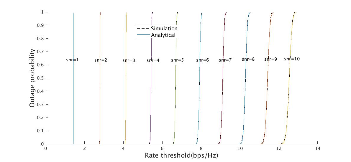
Now, considering equation (1) the Gaussian approximated outage capacity $P_{out}$ can be found as follows

$\displaystyle P_{out}=1-Q\Big{(}\frac{R_{th}-\mathbf{E}\{C\}}{\sqrt{\mathbf{Var}\{C\}}}\Big{)}$
$\displaystyle=Q\Big{(}\frac{\mathbf{E}\{C\}-R_{th}}{\sqrt{\mathbf{Var}\{C\}}}\Big{)}$ (40)

where $Q$ is the tail distribution function of the standard normal distribution and is defined as

$\displaystyle Q(x)=\frac{1}{\sqrt{2\pi}}\int_{x}^{\infty}e^{\frac{-t^{2}}{2}}dt$ (41)

Here, we show the simulation result for outage capacity and we compare it to the one found by (II-B).

Refer to caption
Figure 1: Outage capacity for different number of satellites and receive antenna elements, SNR=10dB. Solid lines and dashed lines represent the outage capacity found by equation (II-B) and simulation, respectively.

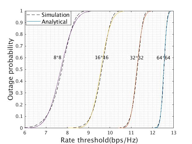
Figure 1 justifies the accuracy of our conjecture.

Refer to caption
Figure 2: Outage capacity of a 64 $\times$ 64 MIMO setup for different SNR’s. Solid lines and dashed lines represent the outage capacity found by equation (II-B) and simulation, respectively.

Appendix A Array factor derivation

The more general form the array factor expression is found using the following expression:

$\displaystyle AF(\theta,\phi)=\sum_{m=0}^{M-1}I_{m}e^{jk\hat{r}.\overrightarrow{r}_{m}}$ (42)

where $\overrightarrow{r}_{m}$ is the position vector to the $m^{th}$ element and $\hat{r}$ is a unit vector pointing in the direction of interest, i.e.,

$\displaystyle\hat{r}=\sin\theta\cos\phi\hat{x}+\sin\theta\sin\phi\hat{y}+\cos\theta\hat{z}$ (43)

and for a linear configuration evenly distributed along y axis with spacing d, $\overrightarrow{r}_{m}=md\hat{y}$. Therefore $\hat{r}.\overrightarrow{r}_{m}=\sin\theta\sin\phi$ and the equation LABEL:eq:4 is derived.

Appendix B Proof of theorem

Characteristic polynomial of an $n\times n$matrix $A$ could be written in terms of traces of matrices $A,A^{2},...,A^{n}$ as follows [13]

$\displaystyle P(\lambda)=b_{0}\lambda^{n}+b_{1}\lambda^{n-1}+b_{2}\lambda^{n-2}+...+b_{n-1}\lambda+b_{n}$ (44)

where

$\displaystyle b_{0}=(-1)^{n},\leavevmode\nobreak\ \leavevmode\nobreak\ \leavevmode\nobreak\ \leavevmode\nobreak\ \leavevmode\nobreak\ \leavevmode\nobreak\ b1=-(-1)^{n}\mathbf{T}_{1}^{A}\leavevmode\nobreak\ \leavevmode\nobreak\ \leavevmode\nobreak\ \leavevmode\nobreak\ \leavevmode\nobreak\ \leavevmode\nobreak\ \leavevmode\nobreak\ \leavevmode\nobreak\ \leavevmode\nobreak\ \leavevmode\nobreak\ \leavevmode\nobreak\ \leavevmode\nobreak$
$\displaystyle b_{2}=-\frac{1}{2}\big{(}b_{1}\mathbf{T}_{1}^{A}+(-1)^{n}\mathbf{T}_{2}^{A}\big{)}\leavevmode\nobreak\ \leavevmode\nobreak\ \leavevmode\nobreak\ \leavevmode\nobreak\ \leavevmode\nobreak\ \leavevmode\nobreak\ \leavevmode\nobreak\ \leavevmode\nobreak\ \leavevmode\nobreak\ \leavevmode\nobreak\ \leavevmode\nobreak\ \leavevmode\nobreak$
$\displaystyle.\leavevmode\nobreak\ \leavevmode\nobreak\ \leavevmode\nobreak\ \leavevmode\nobreak\ \leavevmode\nobreak\ \leavevmode\nobreak\ \leavevmode\nobreak\ \leavevmode\nobreak\ \leavevmode\nobreak\ \leavevmode\nobreak\ \leavevmode\nobreak\ \leavevmode\nobreak\ \leavevmode\nobreak\ \leavevmode\nobreak\ \leavevmode\nobreak\ \leavevmode\nobreak\ \leavevmode\nobreak\ \leavevmode\nobreak\ \leavevmode\nobreak\ \leavevmode\nobreak\ \leavevmode\nobreak\ \leavevmode\nobreak\ \leavevmode\nobreak\ \leavevmode\nobreak$
$\displaystyle b_{n}=-\frac{1}{n}\big{(}b_{n-1}\mathbf{T}_{1}^{A}+b_{n-2}\mathbf{T}_{2}^{A}+...+b_{1}\mathbf{T}_{n-1}+(-1)^{n}\mathbf{T}_{n}^{A}\big{)}$ (45)

and $\mathbf{T}_{1}^{A},\mathbf{T}_{2}^{A},...,\mathbf{T}_{n}^{A}$ denote the traces of matrices $A,A^{2},...,A^{n}$. Also, the summation of roots of equation (46) is equal to $\frac{-b_{1}}{b_{0}}=\mathbf{T}_{1}^{A}$.
On the other hand, eigenvalues of matrix $A^{k}$ are eigenvalues of matrix $A$ each to the power of $k$. Therefore if $\lambda_{1},\lambda_{2},...,\lambda_{n}$ are eigenvalues of matrix $A$, then $\lambda_{1}^{k},\lambda_{2}^{k},...,\lambda_{n}^{k}$ would be those of matrix $A^{k}$, and thus

$\displaystyle\sum_{i=1}^{n}\lambda_{i}^{k}=\mathbf{T}_{1}^{A^{k}}$ (46)

And the theorem is proved.

Appendix C Average channel capacity for a linear array along z axis

The array factor for a linear array along z axis is mentioned in (LABEL:eq:49), where $0\leq\theta\leq\frac{\pi}{2}$. It stands to reason that again $Trace(\mathbf{W})=1$. Using the formula we obtained in (LABEL:eq:23), one can justify that

$\displaystyle\mathbf{E}\Big{\{}Trace(\mathbf{W}^{2})\Big{\}}=\frac{1}{(n_{R}n_{T})^{2}}\Big{(}n_{R}^{2}n_{T}+n_{R}n_{T}(n_{T}-1)+\leavevmode\nobreak\ \leavevmode\nobreak\ \leavevmode\nobreak\ \leavevmode\nobreak\ \leavevmode\nobreak\ \leavevmode\nobreak\ \leavevmode\nobreak\ \leavevmode\nobreak\ \leavevmode\nobreak\ \leavevmode\nobreak\ \leavevmode\nobreak\ \leavevmode\nobreak\ \leavevmode\nobreak$
$\displaystyle 2\sum_{s=1}^{n_{R}-1}(n_{R}-s)n_{T}(n_{T}-1)J_{0}\big{(}\frac{skd}{2}\big{)}^{2}\Big{)}\leavevmode\nobreak\ \leavevmode\nobreak\ \leavevmode\nobreak\ \leavevmode\nobreak\ \leavevmode\nobreak\ \leavevmode\nobreak\ \leavevmode\nobreak\ \leavevmode\nobreak\ \leavevmode\nobreak\ \leavevmode\nobreak\ \leavevmode\nobreak\ \leavevmode\nobreak\ \leavevmode\nobreak$ (47)

Also to obtain the third moment from equation (LABEL:eq:31), we have

$\displaystyle\mathbf{E}\Big{\{}Trace(\mathbf{W}^{2})\Big{\}}=\frac{1}{(n_{R}n_{T})^{3}}\Bigg{(}n_{R}^{3}nT+3n_{R}^{2}n_{T}(n_{T}-1)\leavevmode\nobreak\ \leavevmode\nobreak\ \leavevmode\nobreak\ \leavevmode\nobreak\ \leavevmode\nobreak\ \leavevmode\nobreak$
$\displaystyle+n_{R}n_{T}(n_{T}-1)(n_{T}-2)\leavevmode\nobreak\ \leavevmode\nobreak\ \leavevmode\nobreak\ \leavevmode\nobreak\ \leavevmode\nobreak\ \leavevmode\nobreak\ \leavevmode\nobreak\ \leavevmode\nobreak\ \leavevmode\nobreak\ \leavevmode\nobreak\ \leavevmode\nobreak\ \leavevmode\nobreak$
+6β€‹βˆ‘s=1nRβˆ’1nR​(nRβˆ’s)​nT​(nTβˆ’1)​J0​(s​k​d2)46superscriptsubscript𝑠1subscript𝑛𝑅1subscript𝑛𝑅subscript𝑛𝑅𝑠subscript𝑛𝑇subscript𝑛𝑇1subscript𝐽0superscriptπ‘ π‘˜π‘‘24\displaystyle+6\sum_{s=1}^{n_{R}-1}n_{R}(n_{R}-s)n_{T}(n_{T}-1)J_{0}\big{(}\frac{skd}{2}\big{)}^{4}\leavevmode\nobreak\ \leavevmode\nobreak\ \leavevmode\nobreak\ \leavevmode\nobreak\ \leavevmode\nobreak\ \leavevmode\nobreak\ \leavevmode\nobreak\ \leavevmode\nobreak\ \leavevmode\nobreak\ \leavevmode\nobreak\ \leavevmode\nobreak\ \leavevmode\nobreak\
+6β€‹βˆ‘s=1nRβˆ’1(nTβˆ’2)β€‹βˆk=02(k+s)​J0​((nRβˆ’s)​k​d2)26superscriptsubscript𝑠1subscript𝑛𝑅1subscript𝑛𝑇2superscriptsubscriptproductπ‘˜02π‘˜π‘ subscript𝐽0superscriptsubscriptπ‘›π‘…π‘ π‘˜π‘‘22\displaystyle+6\sum_{s=1}^{n_{R}-1}(n_{T}-2)\prod_{k=0}^{2}(k+s)J_{0}\big{(}\frac{(n_{R}-s)kd}{2}\big{)}^{2}\leavevmode\nobreak\ \leavevmode\nobreak\ \leavevmode\nobreak\ \leavevmode\nobreak\ \leavevmode\nobreak\ \leavevmode\nobreak\ \leavevmode\nobreak\ \leavevmode\nobreak\
+6β€‹βˆ‘s=1nRβˆ’12(nTβˆ’2)β€‹βˆk=02(nRβˆ’2​s+k)​J0​(s​k​d2)4​J0​(s​k​d)6superscriptsubscript𝑠1subscript𝑛𝑅12subscript𝑛𝑇2superscriptsubscriptproductπ‘˜02subscript𝑛𝑅2π‘ π‘˜subscript𝐽0superscriptπ‘ π‘˜π‘‘24subscript𝐽0π‘ π‘˜π‘‘\displaystyle+6\sum_{s=1}^{\frac{n_{R}-1}{2}}(n_{T}-2)\prod_{k=0}^{2}(n_{R}-2s+k)J_{0}\big{(}\frac{skd}{2}\big{)}^{4}J_{0}\big{(}{skd}\big{)}\leavevmode\nobreak\ \leavevmode\nobreak\ \leavevmode\nobreak\ \leavevmode\nobreak\ \leavevmode\nobreak\ \leavevmode\nobreak\ \leavevmode\nobreak\ \leavevmode\nobreak\
$\displaystyle+\Big{(}6\sum_{s=1}^{n_{R}-1}\sum_{t=1}^{n_{R}-2s}(n_{R}-2m)^{+}(n_{T}-2)\times\leavevmode\nobreak\ \leavevmode\nobreak\ \leavevmode\nobreak\ \leavevmode\nobreak\ \leavevmode\nobreak\ \leavevmode\nobreak\ \leavevmode\nobreak\ \leavevmode\nobreak$
$\displaystyle\prod_{k=0}^{2}(2n_{R}-2t-2s+2+k)\times\leavevmode\nobreak\ \leavevmode\nobreak\ \leavevmode\nobreak\ \leavevmode\nobreak\ \leavevmode\nobreak\ \leavevmode\nobreak\ \leavevmode\nobreak\ \leavevmode\nobreak$
$\displaystyle J_{0}\big{(}\frac{skd}{2}\big{)}J_{0}\big{(}\frac{(s+t)kd}{2}\big{)}J_{0}\big{(}\frac{(2s+t)kd}{2}\big{)}\Big{)}\Bigg{)}\leavevmode\nobreak\ \leavevmode\nobreak\ \leavevmode\nobreak\ \leavevmode\nobreak\ \leavevmode\nobreak\ \leavevmode\nobreak\ \leavevmode\nobreak\ \leavevmode\nobreak\ \leavevmode\nobreak$ (48)

References

  • [1] R.Β G. Gallager, Information theory and reliable communication.Β Β Β Springer, 1968, vol.Β 2.
  • [2] C.Β E. Shannon, β€œA mathematical theory of communication,” Bell system technical journal, vol.Β 27, no.Β 3, pp. 379–423, 1948.
  • [3] G.Β E. Corazza, Digital satellite communications.Β Β Β Springer Science & Business Media, 2007.
  • [4] Y.Β W. Liang and B.Β Columbia, β€œErgodic and outage capacity of narrowband mimo gaussian channels,” Dept. of Electrical and computer Engg. University of British Columbia, Vancouver, British Columbia, 2005.
  • [5] R.Β A. Horn and C.Β R. Johnson, Matrix analysis.Β Β Β Cambridge university press, 2012.
  • [6] G.Β H. Tucci and P.Β A. Whiting, β€œEigenvalue results for large scale random vandermonde matrices with unit complex entries,” IEEE Transactions on Information Theory, vol.Β 57, no.Β 6, pp. 3938–3954, 2011.
  • [7] S.Β M. Hamidi, M.Β Mehrabi, A.Β K. Khandani, and D.Β GΓΌndΓΌz, β€œOver-the-air federated learning exploiting channel perturbation,” in 2022 IEEE 23rd International Workshop on Signal Processing Advances in Wireless Communication (SPAWC).Β Β Β IEEE, 2022, pp. 1–5.
  • [8] S.Β M. Hamidi, S.Β Herath, A.Β Bayesteh, and A.Β K. Khandani, β€œSystems and methods for communication resource usage control,” MayΒ 30 2019, uS Patent App. 15/824,352.
  • [9] P.Β Struhsaker, P.Β Posner, S.Β M. Hamidi, and A.Β K. Khandani, β€œMethods for formation of antenna array from sub-arrays,” Aug.Β 25 2020, uS Patent 10,756,443.
  • [10] E.Β Telatar, β€œCapacity of multi-antenna gaussian channels,” European transactions on telecommunications, vol.Β 10, no.Β 6, pp. 585–595, 1999.
  • [11] G.Β J. Foschini and M.Β J. Gans, β€œOn limits of wireless communications in a fading environment when using multiple antennas,” Wireless personal communications, vol.Β 6, no.Β 3, pp. 311–335, 1998.
  • [12] P.Β J. Smith and M.Β Shafi, β€œOn a gaussian approximation to the capacity of wireless mimo systems,” in 2002 IEEE International Conference on Communications. Conference Proceedings. ICC 2002 (Cat. No. 02CH37333), vol.Β 1.Β Β Β IEEE, 2002, pp. 406–410.
  • [13] L.Β L. Pennisi, β€œCoefficients of the characteristic polynomial,” Mathematics magazine, vol.Β 60, no.Β 1, pp. 31–33, 1987.