Learning in Domain Randomization via Continuous
Time Non-Stochastic Control

Abstract

Domain randomization is a popular method for robustly training agents to adapt to diverse environments and real-world tasks. In this paper, we examine how to train an agent in domain randomization environments from a nonstochastic control perspective. We first theoretically study online control of continuous-time linear systems under nonstochastic noises. We present a novel two-level online algorithm, by integrating a higher-level learning strategy and a lower-level feedback control strategy. This method offers a practical solution, and for the first time achieves sublinear regret in continuous-time nonstochastic systems. Compared to standard online learning algorithms, our algorithm features a stack & skip procedure. By applying stack & skip to the SAC (Soft Actor-Critic) algorithm, we achieved improved results in multiple reinforcement learning tasks within domain randomization environments. Our work provides new insights into nonasymptotic analyses of controlling continuous-time systems. Further, our work justifies the importance of stacked & skipped in controller learning under nonstochastic environments.

1 Introduction

A major challenge in robotics is to deploy simulated controllers into real-world systems. This process, known as sim-to-real transfer, can be difficult due to misspecified dynamics, unanticipated real-world perturbations, and non-stationary environments. Various strategies have been proposed to address these issues, including domain randomization, meta-learning, and domain adaptation [32, 11, 5].

In this work, we focus on domain randomization(DR) proposed by [28], which emerges as a pivotal strategy to bridge the sim-to-real gap. This approach focuses on training policies to optimize performance across a wide range of simulated models [30, 18]. In this context, each model’s parameters are randomly sampled from a predetermined task distribution.

The efficacy of DR is particularly notable in its ability to train controllers exclusively within simulated environments, which can then be seamlessly transferred to real world robotic systems [27, 21]. Additionally, the fine-tuning of DR distributions using real-world data, as demonstrated by [16], further enhances its practical applicability and effectiveness.

Although the domain randomization method has shown great effectiveness in experimental results, training agents within a domain randomization environment poses a significant challenge. To accommodate different environments, the strategies developed by agents tend to be overly conservative [15, 2]. Consequently, determining the appropriate distribution of randomization is a challenge, as too much or too little randomization can lead to suboptimal outcomes [31, 16].

Our work starts from the observation that learning in Domain Randomization (DR) differs significantly from stochastic or robust learning problems. In DR, sampling from environmental variables occurs at the beginning of each episode, rather than at every step, distinguishing it from stochastic learning where randomness is step-wise identical and independent. This episodic sampling approach allows agents in DR to exploit environmental conditions and adapt to episodic changes within an episode. On the other hand, robust learning prioritizes worst-case scenarios depending on the an agent’s policy. DR, however, is concerned with the distribution of conditions aimed for broad applicability rather than worst-case perturbations.

Hence, following the research of [1], we provide an analysis of the domain randomization problem from an online non-stochastic control perspective. Online non-stochastic learning problem requires iteratively updating the controller after deployment based on collected trajectories under unknown system perturbations. Significant progress has been made in this field [10, 6, 4]. However, a gap remains as little previous analysis of non-stochastic control has specifically investigated continuous-time systems, but training environments in DR often evolve continuously in time [30, 14, 33].

This work addresses the above problems. Our contributions are summarized below. First, our work analyzes the regret bound for continuous-time online nonstochastic control by studying a two-level controller. The higher-level controller symbolizes the policy learning process and updates the policy at a low frequency to minimize regret. The lower-level controller delivers high-frequency feedback control input to reduce discretization error. We prove the main theorem in Section 5 and our algorithm achieves $O(\sqrt{T}\log(T))$ sublinear regret in time horizon $T$.

Second, we implement the ideas from our theoretical analysis and test them in experiments. We utilize information from past states with some skip to enable faster adaptation to environmental changes. Although the aforementioned concepts are often adopted experimentally as frame stacking and frame skipping, there is relatively little known regarding the appropriate scenarios for applying these techniques. Our analysis and experiments show that these techniques are particularly effective in developing adaptive policy to uncertain environment. Our experiments in domain randomization settings confirm that these techniques substantially improve agents’ rewards.

2 Related Works

Domain randomization

Domain randomization, which is proposed by [28], is a commonly used technique for training agents to adapt to different (real) environments by training in randomized simulated environments. From the empirical perspective, many previous works focus on designing efficient algorithms for learning in a randomized simulated environment (by randomizing environmental settings, such as friction coefficient) such that the algorithm can adapt well in a new environment, [18, 34, 15, 17, 19]. Other works study how to effectively randomize the simulated environment so that the trained algorithm would generalize well in other environments [31, 16, 26]. However, it is unclear why domain randomization works in theory. Limited previous works [5] and [12], have concentrated on theoretically analyzing the sim-to-real gap within specific domain randomization models.

Online non-stochastic control

In online non-stochastic control, the learning algorithm interacts with the environment and updates the policy in each round aiming to achieve sublinear regret with adversarial noise. [1] first studied this setting, and subsequent works studied the adversarial noise with various settings, such as quadratic cost [4], partial observations [24, 23] and unknown dynamical system [10, 6], yielding varying theoretical guarantees like online competitive ratio [8, 22]. Compared to discrete systems, there has been relatively little research on online continuous-time control. Recently, [4] studied online continuous-time linear quadratic control under Brownian noise and unknown system dynamics.

3 Problem Setting

In this section, we first provide a brief introduction to the definitions of stochastic, robust, and non-stochastic control, along with their relationships to the domain randomization setup. We then proceed to introduce the continuous-time non-stochastic control setup.

3.1 Stochastic, Robust Control and Domain Randomization

First, we describe the basic structure of a control problem, which can be viewed as a specific instance of a Markov Decision Process (MDP) with transition dynamics. The state transitions are governed by the following equation:

$$x_{t+1}=f(x_{t},u_{t})+w_{t}\,,$$

where $x_{t}$ denotes the state at time $t$, $u_{t}$ represents the action taken by the controller at time $t$, $f$ is the transition function determining the next state, and $w_{t}$ is the environmental disturbance at time $t$.

The objective of a control problem is to devise an algorithm that outputs a policy $u_{t}=\pi(x_{t})$, aiming to minimize the future cost function for a system with dynamics $f$ and environmental disturbance $w_{t}$. Specifically, for any algorithm $\mathcal{A}$, the cumulative cost over a time horizon $T$ is:

$$J_{T}(\mathcal{A})=\sum_{t=0}^{T}c_{t}(x_{t},u_{t})\,.$$

In the context of stochastic control, as discussed in [7], the disturbance $w_{t}$ follows a distribution $\nu$, with the aim being to minimize the expected cost value:

$$\min_{\mathcal{A}}\mathbb{E}_{w_{t}\sim\nu}[J_{T}(\mathcal{A})].$$ (Stochastic control)

In the realm of robust control, as outlined in [25, 13], the disturbance may adversarially depend on each action taken, leading to the goal of minimizing worst-case cost:

$$\min_{u_{1}}\max_{w_{1:T}}\min_{u_{2}}\ldots\min_{u_{t}}\max_{w_{T}}J_{T}(\mathcal{A}).$$ (Robust control)

We then proceed to establish the framework for domain randomization. When training the agent, we select an environment from the distribution $\nu$ in each episode. Each distinct environment has an associated set of disturbances ${w_{t}}$. However, these disturbances remain fixed once the environment is chosen, unaffected by the agent’s interactions within that environment. Given our limited knowledge about the real-world distribution $\nu$, we focus on optimizing the agent’s performance within its training scope set $\mathcal{V}$. To this end, we aim to minimize the following cost:

$$\min_{\mathcal{A}}\max_{\nu\in\mathcal{V}}\mathbb{E}_{w\sim\nu}[J_{T}(\mathcal{A})].$$ (Domain randomization)

From the aforementioned discussion, it becomes clear that the Domain Randomization (DR) setup diverges significantly from traditional stochastic or robust control. Firstly, unlike in stochastic frameworks, the randomness of disturbance in DR only occurs during the initial environment sampling, rather than at each step of the transition. Secondly, since the system dynamics do not actively counter the controller, this setup does not align with robust control principles.

So how should we analysis DR from a linear control prospective? Notice that [1] also introduces the concept of non-stochastic control. In this context, the disturbance, while not disclosed to the learner beforehand, remains fixed throughout the episode and does not adaptively respond to the control policy. Our goal is to minimize the cost without prior knowledge of the disturbance:

$$\min_{\mathcal{A}}\max_{w_{1:T}}J_{T}(\mathcal{A}).$$ (Non-stochastic control)

In this framework, there’s a clear parallel to domain randomization: fixed yet unknown disturbances in non-stochastic control mirror the unknown training environments in DR. As the agent continually interacts with these environments, it progressively adapts, mirroring the adaptive process seen in domain randomization. Therefore, we propose to study DR from a non-stochastic control perspective.

3.2 Continuous-time Linear Systems and Non-stochastic Continuous Control

Given that training environments in DR often evolve continuously over time and considering the challenges in analyzing nonlinear transitions in $f$, we opt for a continuous-time linear system for theoretical analysis. The transitions and costs in this system are defined as follows:

$$\dot{x}_{t}=Ax_{t}+Bu_{t}+w_{t}\,,\hskip 8.53581ptJ_{T}(\mathcal{A})=\int_{0}^{T}c_{t}(x_{t},u_{t})dt\,.$$

In this framework, we assume that the distribution of $w_{t}$ is fixed, yet unknown to the learner beforehand. The value function of the linear system, represented by the cost $c_{t}(x_{t},u_{t})$, is also not known in advance and is revealed only after the action $u_{t}$ is executed at time $t$. In this continuous-time setup, an online policy $\pi$ is defined as a function mapping known states to actions, i.e., $u_{t}=\pi({x_{\xi}|\xi\in[0,t]})$. Consequently, our objective is to develop an algorithm that formulates such an online policy to minimize the cumulative cost incurred:

$$\min_{\mathcal{A}}\max_{w_{1:T}}J_{T}(\mathcal{A})\,.$$

Although this extension to the setup is a logical progression, the analysis for continuous-time non-stochastic control presents significant differences. As a result, we cannot directly apply the methods used previously, a topic we delve into later in Section 5.

3.3 Assumptions

We operate under the following assumptions throughout this paper. To be concise, we denote $\|\cdot\|$ as the $L_{2}$ norm of the vector and matrix. Firstly, we make assumptions concerning the system dynamics and noise:

Assumption 1.

The matrices that govern the dynamics are bounded, meaning $\|A\|\leq\kappa_{A}$ and $\|B\|\leq\kappa_{B}$, where $\kappa_{A}$ and $\kappa_{B}$ are constants. Moreover, the perturbation and its derivative are both continuous and bounded: $\left\|w_{t}\right\|,\left\|\dot{w}_{t}\right\|\leq W$, with $W$ being a constant.

These assumptions ensure that we can bound the states and actions, as well as their first and second-order derivatives. Next, we make assumptions regarding the cost function:

Assumption 2.

The costs $c_{t}(x,u)$ are convex. Additionally, if there exists a constant $D$ such that $\|x\|,\|u\|\leq D$, then $\left|c_{t}(x,u)\right|\leq\beta D^{2},\left\|\nabla_{x}c_{t}(x,u)\right\|,\left\|\nabla_{u}c_{t}(x,u)\right\|\leq GD$.

This assumption implies that if the differences between states and actions are small, then the error in their cost will also be relatively small. We next describe our baseline policy class which is introduced in [7]:

Definition 1.

A linear policy $K$ is $(\kappa,\gamma)$-strongly stable if, for any $h>0$ that is sufficiently small, there exist matrices $L_{h},P$ such that $I+h(A-BK)=PL_{h}P^{-1}$, with the following two conditions:

1. The norm of $L_{h}$ is strictly smaller than unity and dependent on $h$, i.e., $\|L_{h}\|\leq 1-h\gamma$.

2. The controller and transforming matrices are bounded, i.e., $\|K\|\leq\kappa$ and $\|P\|,\left\|P^{-1}\right\|\leq\kappa$.

The above definition ensures the system can be stabilized by a linear controller $K$.

3.4 Regret formulation

To evaluate the designed algorithm, we follow the setup in [7, 1] and use regret, which is defined as the cumulative difference between the cost incurred by the policy of our algorithm and the cost incurred by the best policy in hindsight. Let $\mathcal{K}$ denotes the class of strongly stable linear policy, i.e. $\mathcal{K}=\{K:K$ is $(\kappa,\gamma)$-strongly stable$\}$. Then we try to minimize the regret of algorithm:

$$\min_{\mathcal{A}}\max_{w_{1:T}}\mathrm{Regret}(\mathcal{A})=\min_{\mathcal{A}}\max_{w_{1:T}}(J_{T}(\mathcal{A})-\min_{K\in\mathcal{K}}J_{T}(K))\,.$$

4 Algorithm Design

In this section, we outline the design of our algorithm, which is built upon a two-level controller update approach. The higher-level controller implements the Online convex optimization with memory [3] framework to sporadically update the policy, while the lower-level controller offers high-frequency control input to minimize discretization error.

Our lower-level controller utilizes the Disturbance-Action policy class(DAC) [1]. We introduce our definition of the DAC policy in the continuous system:

Definition 2.

The Disturbance-Action Policy Class(DAC) and the disturbance are defined as:

$$u_{t}=-Kx_{t}+\sum_{i=1}^{l}M^{i}_{t}\hat{w}_{t-i}\,,\hskip 8.53581pt\hat{w}_{t}=\frac{x_{t+1}-x_{t}-h(Ax_{t}+Bu_{t})}{h}\,.$$ (1)

where $K$ is a fixed strongly stable policy, $l$ is a parameter that signifies the dimension of the policy class, $M_{t}=\{M^{1}_{t},\ldots,M^{l}_{t}\}$ is the weighting parameter of the disturbance at step $t$, and $\hat{w}_{t}$ is the estimated disturbance.

Our higher-level controller adopts the OCO with memory framework. A technical challenge lies in balancing the approximation error and OCO regret. To achieve a low approximation error, we desire the policy update interval $H$ to be inversely proportional to the sampling distance $h$. However, this relationship leads to large OCO regret. To mitigate this issue, we introduce a new parameter $m=\Theta(\frac{1}{h})$, representing the lookahead window. We update the parameter $M_{t}$ only once every $m$ iteration, reducing the OCO regret without negatively impacting the approximation error:

$$M_{t+1}=\left\{\begin{aligned} &\Pi_{\mathcal{M}}\left(M_{t}-\eta\nabla g_{t}(M)\right)&&{\text{if }t\text{ mod }m==0}\,,\\ &M_{t}&&{\text{otherwise}}\,.\end{aligned}\right.$$

For notational convenience, we denote $\tilde{M}_{[t/m]}=M_{t}$. Due to the properties of the OCO with memory structure, we need to consider only the previous $Hm$ states and actions, rather than all states. Then we define the ideal state, action, and cost in the following:

Definition 3.

The ideal state $y_{t}$, action $v_{t}$ and cost $f_{t}$ at time $t\in[im,(i+1)m-1]$ are defined as

$$y_{t}=x_{t}(\tilde{M}_{i-H},...,\tilde{M}_{i}),\hskip 2.84526ptv_{t}=-Ky_{t}+\sum_{j=1}^{l}M_{i}^{j}w_{t-i},\hskip 2.84526ptf_{i}\left(\tilde{M}_{i-H},\ldots,\tilde{M}_{i}\right)=\sum_{t=im}^{(i+1)m-1}c_{t}\left(y_{t},v_{t}\right)\,.$$

where the notation indicates that assume the state $x_{t-H}$ is $0$ and apply the DAC policy $\left(\tilde{M}_{i-H},\ldots,\tilde{M}_{i}\right)$ at all time steps from $t-Hm$ to $t$ and $M^{j}_{i}$ refers to the $j^{th}$ component of vector $M_{i}$.

With all the concepts presented above, we are now prepared to introduce our algorithm:

Algorithm 1 Continuous two-level online control algorithm

  Input: step size $\eta$, sample distance $h$, policy update parameters $H,m$, parameters $\kappa,\gamma,T$.

  Define sample numbers $n=\lceil T/h\rceil$, OCO policy update times $p=\lceil n/m\rceil$.

  Define DAC policy update class $\mathcal{M}=\left\{\tilde{M}=\left\{\tilde{M}^{[1]}\ldots\tilde{M}^{[Hm]}\right\}:\left\|\tilde{M}^{[i]}\right\|\leq 2\kappa^{3}(1-\gamma)^{i-1}\right\}$.

  Initialize $M_{0}\in\mathcal{M}$ arbitrarily.

  for $k=0,\ldots,p-1$ do

     for $s=0,\ldots,m-1$ do

        Denote the discretization time $t=km+s$.

        Use the action $u_{t}=-Kx_{t}+h\sum_{i=1}^{Hm}\tilde{M}_{k}^{i}\hat{w}_{t-i}$ during the time period $[th,(t+1)h]$.

        Observe the new state $x_{t+1}$ at time $(t+1)h$ and update $\hat{w}_{t}$.

     end for

     Define the function $g_{k}(M)=f_{k}(M,\ldots,M)$.

     Update OCO policy $\tilde{M}_{k+1}=\Pi_{\mathcal{M}}\left(\tilde{M}_{k}-\eta\nabla g_{k}(\tilde{M}_{k})\right)$.

  end for

5 Main Result

In this section, we present the primary theorem of online continuous control regret analysis:

Theorem 1.

Under Assumption 1, 2, a step size of $\eta=\Theta(\sqrt{\frac{m}{Th}})$, and a DAC policy update frequency $m=\Theta(\frac{1}{h})$, Algorithm 1 attains a regret bound of

$$J_{T}(\mathcal{A})-\min_{K\in\mathcal{K}}J_{T}(K)\leq O(n(1-h\gamma)^{\frac{H}{h}})+O(\sqrt{nh})+O(Th)\,.$$

With the sampling distance $h=\Theta(\frac{1}{\sqrt{T}})$, and the OCO policy update parameter $H=\Theta(\log(T))$, Algorithm 1 achieves a regret bound of

$$J_{T}(\mathcal{A})-\min_{K\in\mathcal{K}}J_{T}(K)\leq O\left(\sqrt{T}\log\left(T\right)\right)\,.$$

Theorem 1 demonstrates a regret that matches the regret of a discrete system in [1]. We balance discretization error, approximation error, and OCO with memory regret by selecting an appropriate update frequency for the policy. Here, $O(\cdot)$ and $\Theta(\cdot)$ are abbreviations for the polynomial factors of universal constants in the assumption.

Considering the length limit for article submission, the details of the proof can be found at the appendix. We only highlight some proof sketches here.

Key Lemmas in the Proof

We first explain why we cannot directly apply the methods for discrete nonstochastic control from [1] to our work. To utilize Assumption 2, it is necessary first to establish a union bound over the states. In a discrete-time system, it can be easily proved by applying the dynamics inequality $\|x_{t+1}\|\leq a\|x_{t}\|+b$ (where $a<1$) and the induction method presented in [1]. However, for a continuous-time system, a different approach is necessary because we only have the differential equation instead of the state recurrence formula.

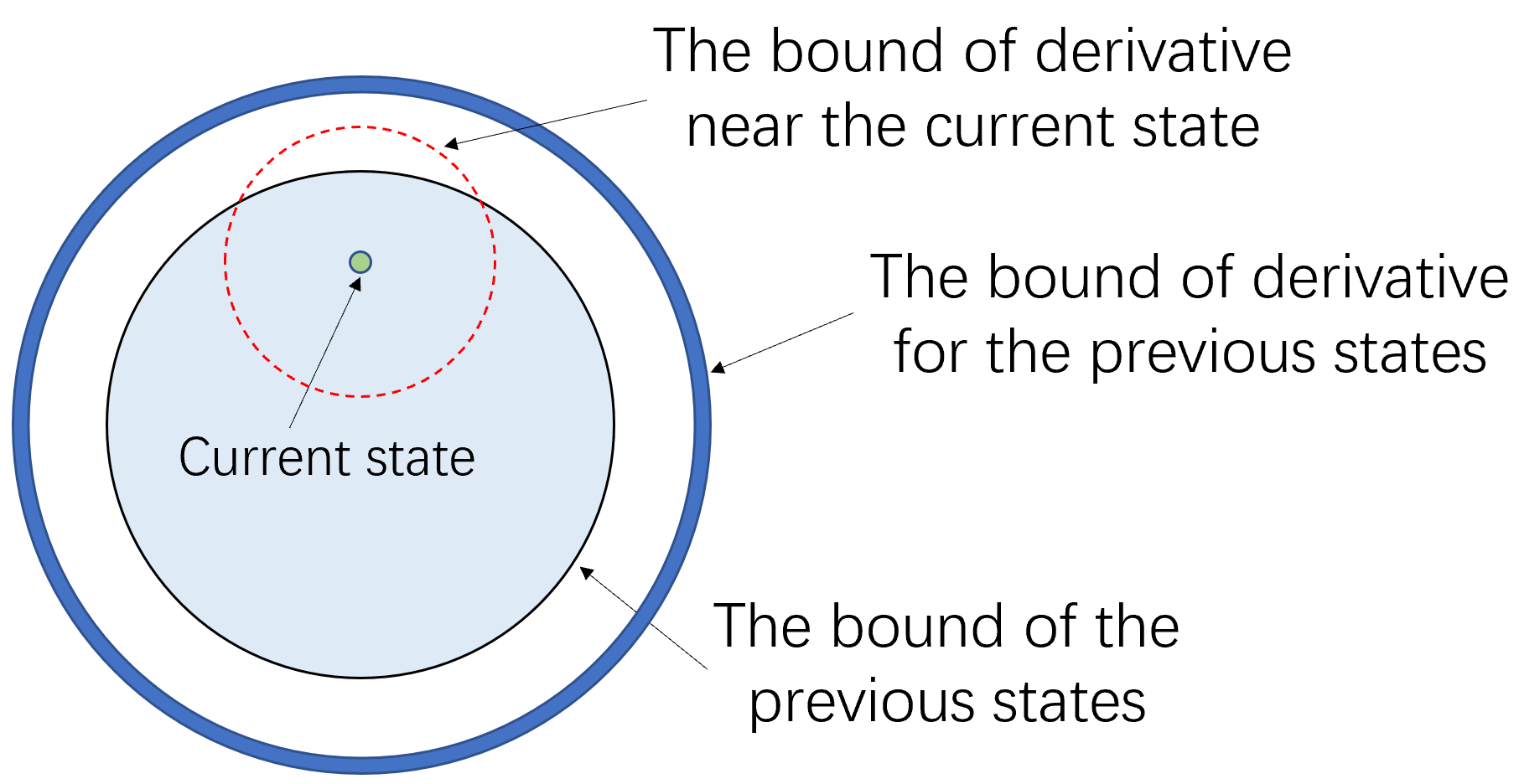
Figure 1: Bounding the states and their derivatives separately.

To overcome this challenge, we employ Gronwall’s inequality to bound the first and second-order derivatives in the neighborhood of the current state. We then use these bounded properties, in conjunction with an estimation of previous noise, to bound the distance to the next state. Through an iterative application of this method, we can argue that all states and actions are bounded.

Another challenge is that we need to discretize the system but we must overcome the curse of dimensionality caused by discretization. In continuous-time systems, the number of states is inversely proportional to the discretization parameter $h$, which also determines the size of the OCO memory buffer. Thus, if we set the OCO memory buffer size as $H=O(\log(T)/h)$ to attain a sublinear ideal cost approximation error $|c_{t}(x_{t},u_{t})-c_{t}(y_{t},v_{t})|$, the associated regret of OCO with memory will be $O(\sqrt{T}/h^{2.5})$. This regret could become excessively large if $h$ is small enough to allow for minimal discretization error. To overcome this problem, we designed a two-level algorithm to reduce the number of policy updates. We only update the policy once in $m=\Theta\left(\frac{1}{h}\right)$ states in the outer level of the algorithm. Therefore, the regret of OCO with memory will be $O(\sqrt{T})$ which is unrelated to $h$ and we finally achieve sublinear regret.

6 Experiments

In this section, we apply our theoretical analysis to the practical training of agents. First we highlight the key difference between our algorithm and traditional online policy optimization.

1. Stack: While standard online policy optimization learns the optimal policy from the current state $u_{t}=\phi(x_{t})$, an optimal non-stochastic controller employs the DAC policy as outlined in equation 1. Leveraging information from past states aids the agent in adapting to dynamic environments.

2. Skip: Different from the analysis in [1], in a continuous-time system we update the state information every few steps, rather than updating it at every step. This solves the curse of dimensionality caused by discretization in continuous-time system.

The above inspires us with an intuitive strategy for training agents by stacking past observations with some observations to skip. We denote this as Stack & skip for convenience. Stack & skip is frequently used as a heuristic in reinforcement learning, yet little was known about when and why such a technique could boost agent performance. Through our theoretical analysis and experiments below, we show that stack & skip should be used when the deployed environments have non-stochastic dynamics, such as domain randomization.

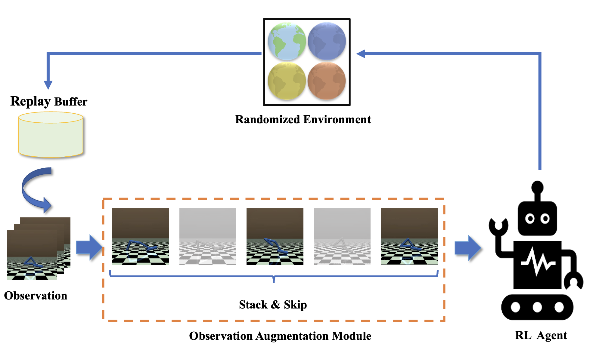
Figure 2: Leverage past observation of states with some skip

Environment	Parameters	DR distribution
Hopper	Joint damping	[0.5, 1.5]
	Foot friction	[1, 3]
	Height of head	[1.2, 1.7]
	Torso size	[0.025, 0.075]
Half-Cheetah	Joint damping	[0.005, 0.015]
	Foot friction	[3, 7]
	Torso size	[0.04, 0.06]
Walker2D	Joint damping	[0.05, 0.15]
	Density	[500, 1500]
	Torso size	[0.025, 0.075]

Table 1: The DR distributions of environment.

Environment Setting

We conduct experiments on the hopper, half-cheetah, and walker2d benchmarks using the MuJoCo simulator [29]. The randomized parameters include environmental physical parameters such as damping and friction, as well as the agent properties such as torso size. We set the range of our domain randomization to follow a distribution with default parameters as the mean value, shown in Table 1. When training in the domain randomization environment, the parameter is uniformly sampled from this distribution. To analyze the result of generalization, we only change one of the parameters and keep the other parameters as the mean of its distribution in each test environment.

Algorithm Design and Baseline

We design a practical meta-algorithm that converts any standard deep RL algorithm into a domain-adaptive algorithm, shown in Figure 2. In this algorithm, we augment the original state observation $o_{t}^{\mathrm{old}}$ at time $t$ with past observations, resulting in $o_{t}^{\mathrm{new}}=[o_{t}^{\mathrm{old}},o_{t-m}^{\mathrm{old}},\ldots,o_{t-(h-1)m}^{\mathrm{old}}]$. Here $h$ is the number of past states we leverage and $m$ is the number of states we skip when we get each of the past states. For clarity in our results, we selected the SAC algorithm for evaluation. We use a variant of Soft Actor-Critic (SAC) [20] and leverage past states with some skip as our algorithm. We compare our algorithm with the standard SAC algorithm training on domain randomization environments as our baseline.

Impact of Frame Stack and Frame Skip

To understand the effects of the frame stack number $h$ and frame skip number $m$, we carried out experiments in the hopper environment with different $h$ and $m$. Figure 4 shows that the performance increases significantly when the frame stack number is increased from $1$ to $3$, and remains roughly unchanged when the frame stack number continues to climb up. Figure 4 shows that the optimal frame skip number is $3$, while both too large or too small frame skip numbers result in sub-optimal results. Therefore, in the following experiments we fix the parameter $h=3$, $m=3$. We train our algorithm with this parameter and standard SAC on hopper and test the performance on more environments. Figure 5 shows that our algorithm outperforms the baseline in all environments.

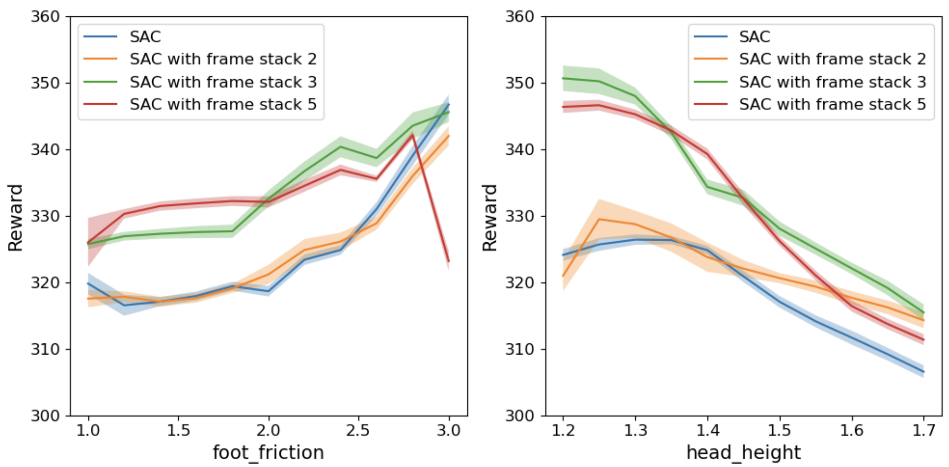
Figure 3: Impact of frame stack number.

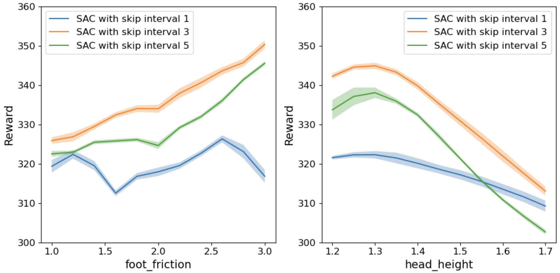
Figure 4: Impact of frame skip number.

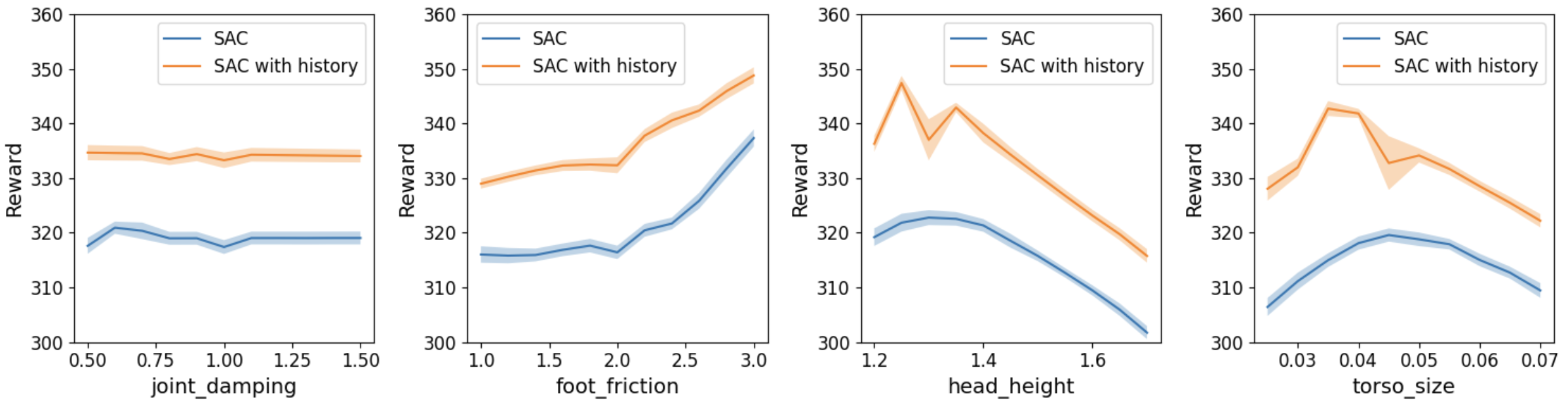
Figure 5: Agents’ reward in various test environments of hopper.

Results on Other Environments

Each algorithm was trained using three distinct random seeds in the half-cheetah and walker2d domain randomization (DR) environments. Consistent with previous experiments, we employed a frame stack number of $h=3$ and frame skip number of $m=3$. The comparative performance of our algorithm and the baseline algorithm, across various domain parameters, is presented in Figure 6. The result clearly demonstrates that our algorithm consistently outperforms the baseline in all evaluated test environments.

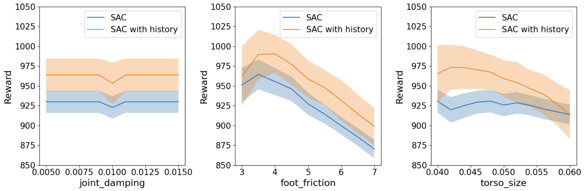
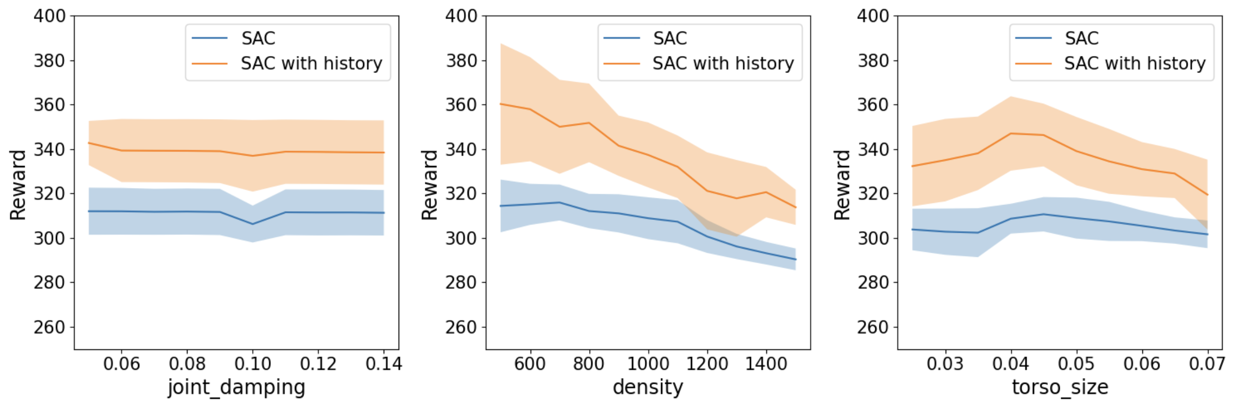
Figure 6: Performance in half-cheetah(Top) and walker2d(Bottom).

7 Conclusions and Future Directions

In this paper, we propose a two-level online controller for continuous-time linear systems with adversarial disturbances, aiming to achieve sublinear regret. This approach is grounded in our examination of agent training in domain randomization environments from an online control perspective. At the higher level, our controller employs the Online Convex Optimization (OCO) with memory framework to update policies at a low frequency, thus reducing regret. The lower level uses the DAC policy to align the system’s actual state more closely with the idealized setting.

In our empirical evaluation, applying our algorithm’s core principles to the SAC (Soft Actor-Critic) algorithm led to significantly improved results in multiple reinforcement learning tasks within domain randomization environments. This highlights the adaptability and effectiveness of our approach in practical scenarios.

For future research, there are several promising directions in online non-stochastic control of continuous-time systems. These include extending our methods to systems with unknown dynamics, exploring the impact of assuming strong convexity in cost functions, and shifting the focus from regret to the competitive ratio. Further research can also explore how to utilize historical information more effectively to enhance agent training in domain randomization environments. This might involve employing time series analysis instead of simply incorporating parameters into neural network training.

In the appendix we define $n$ as the smallest integer greater than or equal to $\frac{T}{h}$, and we use the shorthand $c_{ih}$, $x_{ih}$, $u_{ih}$, and $w_{ih}$ as $c_{i}$, $x_{i}$, $u_{i}$, and $w_{i}$, respectively. First we provide the proof of our main theorem there.

Appendix A Proof of Theorem 1

See 1

Proof.

We denote $u^{\ast}_{t}=K^{\ast}x^{\ast}_{t}$ as the optimal state and action that follows the policy specified by $K^{\ast}$, where $K^{\ast}=\arg\max_{K\in\mathcal{K}}J_{T}(K)$.

We then discretize and decompose the regret as follows:

$$J_{T}(\mathcal{A})-\min_{K\in\mathcal{K}}J_{T}(K) =\int_{0}^{T}c_{t}(x_{t},u_{t})dt-\int_{0}^{T}c_{t}(x^{*}_{t},u^{*}_{t})dt$$

$$=\sum_{i=0}^{n-1}\int_{ih}^{(i+1)h}c_{t}(x_{t},u_{t})dt-\sum_{i=0}^{n-1}\int_{ih}^{(i+1)h}c_{t}(x^{\ast}_{t},u^{\ast}_{t})dt$$

$$=h\left(\sum_{i=0}^{n-1}c_{i}(x_{i},u_{i})-\sum_{i=0}^{n-1}c_{i}(x^{*}_{i},u^{*}_{i})\right)+R_{0}\,,$$

where $R_{0}$ represents the discretization error.

We define $p$ as the smallest integer greater than or equal to $\frac{n}{m}$, then the first term can be further decomposed as

$$\sum_{i=0}^{n-1}c_{i}(x_{i},u_{i})-\sum_{i=0}^{n-1}c_{i}(x^{*}_{i},u^{*}_{i})$$

$$= \sum_{i=0}^{p-1}\sum_{j=im}^{(i+1)m-1}c_{i}(x_{i},u_{i})-\sum_{i=0}^{p-1}\sum_{j=im}^{(i+1)m-1}c_{i}(x^{*}_{i},u^{*}_{i})$$

$$= \sum_{i=0}^{p-1}\left(\sum_{j=im}^{(i+1)m-1}c_{i}(x_{i},u_{i})-\sum_{j=im}^{(i+1)m-1}c_{i}(y_{i},v_{i})\right)+\sum_{i=0}^{p-1}\sum_{j=im}^{(i+1)m-1}c_{i}(y_{i},v_{i})-\sum_{i=0}^{p-1}\sum_{j=im}^{(i+1)m-1}c_{i}(x^{*}_{i},u^{*}_{i})$$

$$= \sum_{i=0}^{p-1}\left(\sum_{j=im}^{(i+1)m-1}c_{i}(x_{i},u_{i})-f_{i}(\tilde{M}_{i-H},\ldots,\tilde{M_{i}})\right)+\sum_{i=0}^{p-1}f_{i}(\tilde{M}_{i-H},\ldots,\tilde{M_{i}})$$

$$-\min_{M\in\mathcal{M}}\sum_{i=0}^{p-1}f_{i}(M,\ldots,M)+\min_{M\in\mathcal{M}}\sum_{i=0}^{p-1}f_{i}(M,\ldots,M)-\sum_{i=0}^{p-1}\sum_{j=im}^{(i+1)m-1}c_{i}(x^{*}_{i},u^{*}_{i})\,,$$

where the last equality is by the definition of the idealized cost function.

Let us denote

$$R_{1}=\ \sum_{i=0}^{p-1}\left(\sum_{j=im}^{(i+1)m-1}c_{i}(x_{i},u_{i})-f_{i}(\tilde{M}_{i-H},\ldots,\tilde{M_{i}})\right)\,,$$

$$R_{2}=\ \sum_{i=0}^{p-1}f_{i}(\tilde{M}_{i-H},\ldots,\tilde{M_{i}})-\min_{M\in\mathcal{M}}\sum_{i=0}^{p-1}f_{i}(M,\ldots,M)\,,$$

$$R_{3}=\ \min_{M\in\mathcal{M}}\sum_{i=0}^{p-1}f_{i}(M,\ldots,M)-\sum_{i=0}^{p-1}\sum_{j=im}^{(i+1)m-1}c_{i}(x^{*}_{i},u^{*}_{i})\,.$$

Then we have the regret decomposition as

$$\mathrm{Regret}(T)=h(R_{1}+R_{2}+R_{3})+O(hT)\,.$$

We then separately upper bound each of the four terms.

The term $R_{0}$ represents the error caused by discretization, which decreases as the number of sampling points increases and the sampling distance $h$ decreases. This is because more sampling points make our approximation of the continuous system more accurate. Using Lemma 3, we get the following upper bound: $R_{0}\leq O(hT)$.

The term $R_{1}$ represents the difference between the actual cost and the approximate cost. For a fixed $h$, this error decreases as the number of sample points looked ahead $m$ increases, while it increases as the sampling distance $h$ decreases. This is because the closer adjacent points are, the slower the convergence after approximation. By Lemma 4 we can bound it as $R_{1}\leq O(n(1-h\gamma)^{Hm})$.

The term $R_{2}$ is incurred due to the regret of the OCO with memory algorithm. Note that this term is determined by learning rate $\eta$ and the policy update frequency $m$. Choosing suitable parameters and using Lemma 5, we can obtain the following upper bound: $R_{2}\leq O(\sqrt{n/h})$.

The term $R_{3}$ represents the difference between the ideal optimal cost and the actual optimal cost. Since the accuracy of the DAC policy approximation of the optimal policy depends on its degree of freedom $l$, a higher degree of freedom leads to a more accurate approximation of the optimal policy. We use Lemma 6 and choose $l=Hm$ to bound this error: $R_{3}\leq O(n(1-h\gamma)^{Hm})$.

By summing up these four terms and taking $m=\Theta(\frac{1}{h})$, we get:

$$\text{Regret}(T)\leq O(nh(1-h\gamma)^{\frac{H}{h}})+O(\sqrt{nh})+O(hT)\,.$$

Finally, we choose $h=\Theta\left(\frac{1}{\sqrt{T}}\right)$, $m=\Theta\left(\frac{1}{h}\right)$, $H=\Theta(log(T))$, the regret is bounded by

$$\text{Regret}(T)\leq O(\sqrt{T}\log(T))\,.$$

∎

Appendix B Key Lemmas

In this section, we will primarily discuss the rationale behind the proof of our key lemmas.

Bounding the States and Actions

First, we need to prove all the states and actions are bounded.

Lemma 2.

Under Assumption 1 and 2, choosing arbitrary $h$ in the interval $[0,h_{0}]$ where $h_{0}$ is a constant only depends on the parameters in the assumption, we have for any $t$ and policy $M_{i}$, $\|x_{t}\|,\|y_{t}\|,\|u_{t}\|,\|v_{t}\|\leq D$. $\|x_{t}-y_{t}\|,\|u_{t}-v_{t}\|\leq\kappa^{2}(1+\kappa)(1-h\gamma)^{Hm+1}D$. In particular, taking all the $M_{t}=0$ and $K=K^{*}$, we obtain the actual optimal solution $\|x^{*}_{t}\|,\|u^{*}_{t}\|\leq D$.

The proof of this Lemma mainly use the Gronwall inequality and the induction method.

Then we analyze the discretization error of the system.

Bounding the Discretization Error

Analyzing a continuous system can be arduous; hence, we employ discretization with distance $h$ to facilitate the analysis.

Lemma 3.

Under Assumption 2, Algorithm 1 attains the following bound of $R_{0}$:

$$R_{0}=\sum_{i=0}^{n-1}\int_{ih}^{(i+1)h}(c_{t}(x_{t},u_{t})-c_{t}(x^{\ast}_{t},u^{\ast}_{t}))dt-h\sum_{i=0}^{n-1}\left(c_{i}(x_{i},u_{i})-c_{i}(x^{*}_{i},u^{*}_{i})\right)\leq 2GDhT\,.$$

This lemma indicates that the discretization error is directly proportional to the sample distance $h$. In other words, increasing the number of sampling points leads to more accurate estimation of system.

Based on Lemma 2, we know that $\|x_{t}\|,\|u_{t}\|\leq D$. By utilizing assumption 2, we can deduce that:

$$|c_{t}(x_{t},u_{t})-c_{ih}(x_{ih},u_{ih})|\leq\max_{x,u}(\left\|\nabla_{x}c_{t}(x,u)\right\|+\left\|\nabla_{u}c_{t}(x,u)\right\|)(t-ih)\leq GD(t-ih)\,.$$

Summing up all these terms, we obtain the bound for the discretization error.

Bounding the Difference between Ideal Cost and Actual Cost

The following lemma describes the upper bound of the error by approximating the ideal state and action:

Lemma 4.

Under Assumption 1 and 2, Algorithm 1 attains the following bound of $R_{1}$:

$$R_{1}=\ \sum_{i=0}^{p-1}\left(\sum_{j=im}^{(i+1)m-1}c_{i}(x_{i},u_{i})-f_{i}\left(\tilde{M}_{i-H},\ldots,\tilde{M_{i}}\right)\right)\leq nGD^{2}\kappa^{2}(1+\kappa)(1-h\gamma)^{Hm+1}\,.$$

From this lemma, it is evident that for a fixed sample distance $h$, the error diminishes as the number of sample points looked ahead $m$ increases. However, as the sampling distance $h$ decreases, the convergence rate of this term becomes slower. Therefore, it is not possible to select an arbitrarily small value for $h$ in order to minimize the discretization error $R_{0}$.

We need to demonstrate that the discrepancy between $x_{t}$ and $y_{t}$, as well as $u_{t}$ and $v_{t}$, is sufficiently small, given assumption 1. This can be proven by analyzing the state evolution under the DAC policy.

By utilizing Assumption 2 and Lemma 2, we can deduce the following inequality:

$$\left|c_{t}\left(x_{t},u_{t}\right)-c_{t}\left(y_{t},v_{t}\right)\right|\leq\ \left|c_{t}\left(x_{t},u_{t}\right)-c_{t}\left(y_{t},u_{t}\right)\right|+\left|c_{t}\left(y_{t},u_{t}\right)-c_{t}\left(y_{t},v_{t}\right)\right|$$

$$\leq\ GD\|x_{t}-y_{t}\|+GD\|u_{t}-v_{t}\|\,.$$

Summing over all the terms and use Lemma 2, we can derive an upper bound for $R_{1}$.

Next, we analyze the regret of Online Convex Optimization (OCO) with a memory term.

Bounding the Regret of OCO with Memory

To analyze OCO with a memory term, we provide an overview of the framework established by [3] in online convex optimization. The framework considers a scenario where, at each time step $t$, an online player selects a point $x_{t}$ from a set $\mathcal{K}\subset\mathbb{R}^{d}$. At each time step, a loss function $f_{t}:\mathcal{K}^{H+1}\rightarrow\mathbb{R}$ is revealed, and the player incurs a loss of $f_{t}\left(x_{t-H},\ldots,x_{t}\right)$. The objective is to minimize the policy regret, which is defined as

$$\mathrm{PolicyRegret}=\sum_{t=H}^{T}f_{t}\left(x_{t-H},\ldots,x_{t}\right)-\min_{x\in\mathcal{K}}\sum_{t=H}^{T}f_{t}(x,\ldots,x)\,.$$

In this setup, the first term corresponds to the DAC policy we choose, while the second term is used to approximate the optimal strongly stable linear policy.

Lemma 5.

Under Assumption 1 and 2, choosing $m=\frac{C}{h}$ and $\eta=\Theta(\frac{m}{Th})$, Algorithm 1 attains the following bound of $R_{2}$:

$$R_{2} =\sum_{i=0}^{p-1}f_{i}(\tilde{M}_{i-H},\ldots,\tilde{M_{i}})-\min_{M\in\mathcal{M}}\sum_{i=0}^{p-1}f_{i}(M,\ldots,M)$$

$$\leq\frac{4a}{\gamma}\sqrt{\frac{GDC^{2}\kappa^{2}(\kappa+1)W_{0}\kappa_{B}}{\gamma}(\frac{GDC\kappa^{2}(\kappa+1)W_{0}\kappa_{B}}{\gamma}+C^{2}\kappa^{3}\kappa_{B}W_{0}H^{2})\frac{n}{h}}\,.$$

To analyze this term, we can transform the problem into an online convex optimization with memory and utilize existing results presented by [3] for it. By applying their results, we can derive the following bound:

$$\sum_{t=H}^{T}f_{t}\left(x_{t-H},\ldots,x_{t}\right)-\min_{x\in\mathcal{K}}\sum_{t=H}^{T}f_{t}(x,\ldots,x)\leq O\left(D\sqrt{G_{f}\left(G_{f}+LH^{2}\right)T}\right)\,.$$

Taking into account the bounds on the diameter, Lipschitz constant, and the gradient, we can ultimately derive an upper bound for $R_{2}$.

Bounding the Approximation Error of DAC Policy

Lastly, we aim to establish a bound on the approximation error between the optimal DAC policy and the unknown optimal linear policy.

Lemma 6.

Under Assumption 1 and 2, Algorithm 1 attains the following bound of $R_{3}$:

$$R_{3} =\min_{M\in\mathcal{M}}\sum_{i=0}^{p-1}f_{i}(M,...,M)-\sum_{i=0}^{p-1}\sum_{j=im}^{(i+1)m-1}c_{i}(x^{*}_{i},u^{*}_{i})\leq 3n(1-h\gamma)^{Hm}GDW_{0}\kappa^{3}a(lh\kappa_{B}+1)\,.$$

The intuition behind this lemma is that the evolution of states leads to an approximation of the optimal linear policy in hindsight, where $u_{t}^{*}=-K^{*}x_{t}$ if we choose $M^{*}=\{M^{i}\}$, where $M^{i}=(K-K^{*})(I+h(A-BK^{*}))^{i}$. Although the optimal policy $K^{*}$ is unknown, such an upper bound is attainable because the left-hand side represents the minimum of $M\in\mathcal{M}$.

Appendix C The evolution of the state

In this section we will prove that using the DAC policy, the states and actions are uniformly bounded. The difference between ideal and actual states and the difference between ideal and actual action is very small.

We begin with expressions of the state evolution using DAC policy:

Lemma 7.

We have the evolution of the state and action:

$$x_{t+1}=\ Q^{l+1}_{h}x_{t-l}+h\sum_{i=0}^{2l}\Psi_{t,i}\hat{w}_{t-i}\,,$$

$$y_{t+1}=\ h\sum_{i=0}^{2Hm}\Psi_{t,i}\hat{w}_{t-i}\,,$$

$$v_{t}=\ -Ky_{t}+h\sum_{j=1}^{Hm}M_{t}^{j}\hat{w}_{t-j}\,.$$

where $\Psi_{t,i}$ represent the coefficients of $\hat{w}_{t-i}$:

$$\Psi_{t,i}=Q^{i}_{h}\mathbf{1}_{i\leq l}+h\sum_{j=0}^{l}Q^{j}_{h}BM_{t-j}^{i-j}\mathbf{1}_{i-j\in[1,l]}\,.$$

Proof.

Define $Q_{h}=I+h(A-BK)$. Using the Taylor expansion of $x_{t}$ and denoting $r_{t}$ as the second-order residue term, we have

$$x_{t+1}=x_{t}+h\dot{x}_{t}+h^{2}r_{t}=x_{t}+h(Ax_{t}+Bu_{t}+w_{t})+h^{2}r_{t}\,.$$

Then we calculate the difference between $w_{i}$ and $\hat{w}_{i}$:

$$\hat{w}_{t}-w_{t}=\frac{x_{t+1}-x_{t}-h(Ax_{t}+Bu_{t}+w_{t})}{h}=hr_{t}\,.$$

Using the definition of DAC policy and the difference between disturbance, we have

$$x_{t+1} =x_{t}+h\left(Ax_{t}+B\left(-Kx_{t}+h\sum_{i=1}^{l}M_{t}^{i}\hat{w}_{t-i}\right)+\hat{w}_{t}-hr_{t}\right)+h^{2}r_{t}$$

$$=(I+h(A-BK))x_{t}+h\left(Bh\sum_{i=1}^{l}M_{t}^{i}\hat{w}_{t-i}+\hat{w}_{t}\right)$$

$$=Q_{h}x_{t}+h\left(Bh\sum_{i=1}^{l}M_{t}^{i}\hat{w}_{t-i}+\hat{w_{t}}\right)$$

$$=Q^{2}_{h}x_{t-1}+h\left(Q_{h}\left(Bh\sum_{i=1}^{l}M_{t-1}^{i}\hat{w}_{t-1-i}+\hat{w}_{t-1}\right)\right)+h\left(Bh\sum_{i=1}^{l}M_{t}^{i}\hat{w}_{t-i}+\hat{w_{t}}\right)$$

$$=Q^{l+1}_{h}x_{t-l}+h\sum_{i=0}^{2l}\Psi_{t,i}\hat{w}_{t-i}\,,$$

where the last equality is by recursion and $\Psi_{t,i}$ represent the coefficients of $\hat{w}_{t-i}$.

Then we calculate the coefficients of $w_{t-i}$ and get the following result:

$$\Psi_{t,i}=Q^{i}_{h}\mathbf{1}_{i\leq l}+h\sum_{j=0}^{l}Q^{j}_{h}BM_{t-j}^{i-j}\mathbf{1}_{i-j\in[1,l]}\,.$$

By the ideal definition of $y_{t+1}$ and $v_{t}$(only consider the effect of the past $Hm$ steps while planning, assume $x_{t-Hm}=0$), taking $l=Hm$ we have

$$y_{t+1}=\ h\sum_{i=0}^{2Hm}\Psi_{t,i}\hat{w}_{t-i},$$

$$v_{t}=\ -Ky_{t}+h\sum_{j=1}^{Hm}M_{t}^{j}\hat{w}_{t-j}\,.$$ ∎

Then we prove the norm of the transition matrix is bounded.

Lemma 8.

We have the following bound of the transition matrix:

$$\left\|\Psi_{t,i}\right\|\leq a(lh\kappa_{B}+1)\kappa^{2}(1-h\gamma)^{i-1}\,.$$

Proof.

By the definition of strongly stable policy, we know

$$\|Q^{i}_{h}\|=\|(PL_{h}P^{-1})^{i}\|=\|P(L_{h})^{i}P^{-1}\|\leq\|P\|\|L_{h}\|^{i}\|P^{-1}\|\leq a\kappa^{2}(1-h\gamma)^{i}\,.$$ (2)

By the definition of $\Psi_{t,i}$, we have

$$\left\|\Psi_{t,i}\right\| =\left\|Q^{i}_{h}\mathbf{1}_{i\leq l}+h\sum_{j=0}^{l}Q^{j}_{h}BM_{t-j}^{i-j}\mathbf{1}_{i-j\in[1,l]}\right\|$$

$$\leq\kappa^{2}(1-h\gamma)^{i}+ah\sum_{j=1}^{l}\kappa_{B}\kappa^{2}(1-h\gamma)^{j}(1-h\gamma)^{i-j-1}$$

$$\leq\kappa^{2}(1-h\gamma)^{i}+alh\kappa_{B}\kappa^{2}(1-h\gamma)^{i-1}\leq a(lh\kappa_{B}+1)\kappa^{2}(1-h\gamma)^{i-1}\,,$$

where the first inequality is due to equation 2, assumption 1 and the condition of $\left\|M_{t}^{i}\right\|\leq a(1-h\gamma)^{i-1}$. ∎

After that, we can uniformly bound the state $x_{t}$ and its first and second-order derivative.

Lemma 9.

For any $t\in[0,T]$, choosing arbitrary $h$ in the interval $[0,h_{0}]$ where $h_{0}$ is a constant only depends on the parameters in the assumption, we have $\|x_{t}\|\leq D_{1}$, $\|\dot{x}_{t}\|\leq D_{2}$, $\|\ddot{x}_{t}\|\leq D_{3}$ and the estimatation of disturbance is bounded by $\|\hat{w}_{t}\|\leq W_{0}$. Moreover, $D_{1}$, $D_{2}$, $D_{3}$ are only depend on the parameters in the assumption.

Proof.

We prove this lemma by induction. When $t=0$, it is clear that $x_{0}$ satisfies this condition. Suppose $x_{t}\leq D_{1}$, $\dot{x}_{t}\leq D_{2}$, $\ddot{x}_{t}\leq D_{3}$, $\hat{w}_{t}\leq W_{0}$ for any $t\leq t_{0}$, where $t_{0}=kh$ is the $k$-th discretization point. Then for $t\in[t_{0},t_{0}+h]$, we first prove that $\dot{x}_{t}\leq D_{2}$, $\ddot{x}_{t}\leq D_{3}$.

By Assumption 1 and our definition of $u_{t}$, we know that for any $t\in[t_{0},t_{0}+h]$. Thus, we have

$$\|\dot{x}_{t}\| =\|Ax_{t}+Bu_{t}+w_{t}\|$$

$$=\|Ax_{t}+B(-Kx_{t_{0}}+h\sum_{i=1}^{l}M^{i}_{k}\hat{w}_{k-i})+w_{t}\|$$

$$\leq\kappa_{A}\|x_{t}\|+\kappa_{B}\kappa\|x_{t_{0}}\|+h\sum_{i=1}^{l}(1-h\gamma)^{i-1}W_{0}+W$$

$$\leq\kappa_{A}\|x_{t}\|+\kappa_{B}\kappa D_{1}+\frac{W_{0}}{\gamma}+W\,,$$

where the first inequality is by the induction hypothesis $\hat{w}_{t}\leq W_{0}$ for any $t\leq t_{0}$ and $M^{i}_{k}\leq(1-h\gamma)^{i-1}$, the second inequality is by the induction hypothesis $x_{t}\leq D_{1}$ for any $t\leq t_{0}$.

For any $t\in[t_{0},t_{0}+h]$, because we choose the fixed policy $u_{t}\equiv u_{t_{0}}$, so we have $\dot{u}_{t}=0$ and

$$\|\ddot{x}_{t}\| =\|A\dot{x}_{t}+B\dot{u}_{t}+w_{t}\|=\|A\dot{x}_{t}+w_{t}\|\leq\kappa_{A}\|\dot{x}_{t}\|+W\,.$$

By the Newton-Leibniz formula, we have for any $\zeta\in[0,h]$,

$$\dot{x}_{t_{0}+\zeta}-\dot{x}_{t_{0}}=\int_{0}^{\zeta}\ddot{x}_{t_{0}+\xi}d_{\xi}\,.$$

Then we have

$$\|\dot{x}_{t_{0}+\zeta}\| \leq\|\dot{x}_{t_{0}}\|+\int_{0}^{\zeta}\|\ddot{x}_{t_{0}+\xi}\|d_{\xi}$$

$$\leq\|\dot{x}_{t_{0}}\|+\int_{0}^{\zeta}(\kappa_{A}\|\dot{x}_{t_{0}+\xi}\|+W)d_{\xi}$$

$$=\|\dot{x}_{t_{0}}\|+W\zeta+\kappa_{A}\int_{0}^{\zeta}\|\dot{x}_{t_{0}+\xi}\|d_{\xi}\,.$$

By Gronwall inequality, we have

$$\|\dot{x}_{t_{0}+\zeta}\| \leq\|\dot{x}_{t_{0}}\|+W\zeta+\int_{0}^{\zeta}(\|\dot{x}_{t_{0}}\|+W\xi)\exp(\kappa_{A}(\zeta-\xi))d_{\xi}\,.$$

Then we have

$$\|\dot{x}_{t_{0}+\zeta}\| \leq\|\dot{x}_{t_{0}}\|+W\zeta+\int_{0}^{\zeta}(\|\dot{x}_{t_{0}}\|+W\zeta)\exp(\kappa_{A}\zeta))d_{\xi}$$

$$=(\|\dot{x}_{t_{0}}\|+W\zeta)(1+\zeta\exp(\kappa_{A}\zeta))$$

$$\leq\left(\kappa_{A}\|x_{t_{0}}\|+\kappa_{B}\kappa D_{1}+\frac{W_{0}}{\gamma}+W+Wh\right)(1+h\exp(\kappa_{A}h))$$

$$\leq\left((\kappa_{A}+\kappa_{B}\kappa)D_{1}+\frac{W_{0}}{\gamma}+W+Wh\right)(1+h\exp(\kappa_{A}h))$$

$$\leq\left((\kappa_{A}+\kappa_{B}\kappa)D_{1}+\frac{W_{0}}{\gamma}+2W\right)(1+\exp(\kappa_{A}))\,,$$

where the first inequality is by the relation $\xi\leq\zeta$, the second inequality is by the relation $\zeta\leq h$ and the bounding property of first-order derivative, the third inequality is by the induction hypothesis and the last inequality is due to $h\leq 1$.

By the relation $\|\ddot{x}_{t}\|\leq\kappa_{A}\|\dot{x}_{t}\|+W$, we have

$$\|\ddot{x}_{t_{0}+\zeta}\| \leq\kappa_{A}D_{2}+W\,.$$

So we choose $D_{3}=\kappa_{A}D_{2}+W$. By the equation, we have

$$\|\hat{w}_{t}-w_{t}\| =\left\|\frac{x_{t+1}-x_{t}-h(Ax_{t}+Bu_{t}+w_{t})}{h}\right\|$$

$$=\left\|\frac{x_{t+1}-x_{t}-h\dot{x}_{t}}{h}\right\|=\left\|\frac{\int_{0}^{h}(\dot{x}_{t+\xi}-\dot{x}_{t})d\xi}{h}\right\|=\left\|\frac{\int_{0}^{h}\int_{0}^{\xi}\ddot{x}_{t+\zeta}d\zeta d\xi}{h}\right\|$$

$$\leq\frac{\int_{0}^{h}\int_{0}^{\xi}\|\ddot{x}_{t+\zeta}\|d\zeta d\xi}{h}$$

$$\leq hD_{3}\,,$$

where in the second line we use the Newton-Leibniz formula, the inequality is by the conclusion $\|\ddot{x}_{t}\|\leq D_{3}$ which we have proved before. By Assumption 1, we have

$$\|\hat{w}_{t}\|\leq W+hD_{3}\,.$$

Choosing $D_{3}=\kappa_{A}D_{2}+W$, $W_{0}=W+hD_{3}=W+h(\kappa_{A}D_{2}+W)$, we get

$$\|\dot{x}_{t_{0}+\zeta}\| \leq((\kappa_{A}+\kappa_{B}\kappa)D_{1}+\frac{W_{0}}{\gamma}+2W)(1+\exp(\kappa_{A}))$$

$$\leq((\kappa_{A}+\kappa_{B}\kappa)D_{1}+\frac{W+h(\kappa_{A}D_{2}+W)}{\gamma}+2W)(1+\exp(\kappa_{A}))$$

$$\leq D_{2}\left(\frac{h\kappa_{A}}{\gamma}(1+\exp(\kappa_{A}))\right)+\left((\kappa_{A}+\kappa_{B}\kappa)D_{1}+\frac{(1+h+2\gamma)W}{\gamma}\right)(1+\exp(\kappa_{A})))\,.$$

Using the notation

$$\beta_{1} =\frac{h\kappa_{A}}{\gamma}(1+\exp(\kappa_{A}))\,,$$

$$\beta_{2} =\left((\kappa_{A}+\kappa_{B}\kappa)D_{1}+\frac{2(1+\gamma)W}{\gamma}\right)(1+\exp(\kappa_{A}))\,.$$

When $h<\frac{\gamma}{2\kappa_{A}(1+\exp(\kappa_{A}))}$, we have $\beta_{1}<\frac{1}{2}$. Taking $D_{2}=2\beta_{2}$ we get

$$\|\dot{x}_{t_{0}+\zeta}\| \leq\beta_{1}D_{2}+\beta_{2}\leq D_{2}\,.$$

So we have proved that for any $t\in[t_{0},t_{0}+h]$, $\|\dot{x}_{t}\|\leq D_{2}$, $\|\ddot{x}_{t}\|\leq D_{3}$, $\|\hat{w}_{t}\|\leq W_{0}$.

Then we choose suitable $D_{1}$ and prove that for any $t\in[t_{0},t_{0}+h]$, $\|x_{t}\|\leq D_{1}$.

Using Lemma 7, we have

$$x_{t+1} =h\sum_{i=0}^{t}\Psi_{t,i}\hat{w}_{t-i}\,.$$

By the induction hypothesis of bounded state and estimation noise in $[0,t_{0}]$ together with Lemma 8, we have

$$\|x_{t+1}\| \leq h\sum_{i=0}^{t}(lh\kappa_{B}+1)\kappa^{2}(1-h\gamma)^{i}(W+hD_{3})$$

$$\leq\frac{(lh\kappa_{B}+1)\kappa^{2}(W+hD_{3})}{\gamma}\,.$$

Then, by the Taylor expansion and the inequality $\dot{x}_{t}\leq D_{2}$ , we have for any $\zeta\in[0,h]$,

$$\|x_{t+1}-x_{t+\zeta}\| =\|\int^{h}_{\zeta}\dot{x}_{t+\xi}d\xi\|\leq(h-\zeta)D_{2}\leq hD_{2}\,.$$

Therefore we have

$$\|x_{t+\zeta}\| \leq\|x_{t+1}\|+hD_{2}\leq\frac{(lh\kappa_{B}+1)\kappa^{2}(W+hD_{3})}{\gamma}+hD_{2}$$

$$=\frac{(lh\kappa_{B}+1)\kappa^{2}W(1+h)}{\gamma}+hD_{2}\left(\frac{(lh\kappa_{B}+1)\kappa^{2}\kappa_{A}}{\gamma}+1\right)$$

$$\leq\frac{(l\kappa_{B}+1)2\kappa^{2}W}{\gamma}+hD_{2}\left(\frac{(l\kappa_{B}+1)\kappa^{2}\kappa_{A}}{\gamma}+1\right)\,.$$

In the last inequality we use $h\leq 1$.

By the relation $D_{2}=\beta_{2}/(1-\beta_{1})$ and $\beta_{1}\leq\frac{1}{2}$, we know that

$$D_{2}\leq 2\left((\kappa_{A}+\kappa_{B}\kappa)D_{1}+\frac{2(1+\gamma)W}{\gamma}\right)(1+\exp(\kappa_{A})).$$

Using the notation

$$\gamma_{1} =2h(\kappa_{A}+\kappa_{B}\kappa)(1+\exp(\kappa_{A}))\,,$$

$$\gamma_{2} =\frac{(l\kappa_{B}+1)2\kappa^{2}W}{\gamma}+4\frac{(1+\gamma)W}{\gamma}(1+\exp(\kappa_{A}))\left(\frac{(l\kappa_{B}+1)\kappa^{2}\kappa_{A}}{\gamma}+1\right)\,.$$

We have $\|x_{t+\zeta}\|\leq\gamma_{1}D_{1}+\gamma_{2}$.

From the equation of $\gamma_{1}$ we know that when $h\leq\frac{1}{4(\kappa_{A}+\kappa_{B}\kappa)(1+\exp(\kappa_{A}))}$ we have $\gamma_{1}\leq\frac{1}{2}$. Then we choose $D_{1}=2\gamma_{2}$, we finally get

$$\|x_{t+\zeta}\| \leq\gamma_{1}D_{1}+\gamma_{2}\leq D_{1}\,.$$

Finally, set

$$h_{0}=\min\left\{1,\frac{\gamma}{\kappa_{A}(1+\exp(\kappa_{A}))},\frac{1}{4(\kappa_{A}+\kappa_{B}\kappa)(1+\exp(\kappa_{A}))}\right\}\,,$$

By the relationship $D_{1}=2\gamma_{2}$, $D_{2}=2\beta_{2}$, $D_{3}=\kappa_{A}D_{2}+W$, $W_{0}=W+hD_{3}$,

we can verify the induction hypothesis. Moreover, we know that $D_{1}$, $D_{2}$, $D_{3}$ are not depend on $h$. Therefore we have proved the claim.

∎

The last step is then to bound the action and the approximation errors of states and actions.

See 2

Proof.

By Lemma 8, we have

$$\left\|\Psi_{t,i}\right\|\leq a(lh\kappa_{B}+1)\kappa^{2}(1-h\gamma)^{i-1}\,.$$

By Lemma 9 we know that for any $h$ in $[0,h_{0}]$, where

$$h_{0}=\min\left\{1,\frac{\gamma}{\kappa_{A}(1+\exp(\kappa_{A}))},\frac{1}{4(\kappa_{A}+\kappa_{B}\kappa)(1+\exp(\kappa_{A}))}\right\}\,,$$

we have $\|x_{t}\|\leq D_{1}$.

By Lemma 7, Lemma 8 and Lemma 9, we have

$$\|y_{t+1}\| =\|h\sum_{i=0}^{2Hm}\Psi_{t,i}\hat{w}_{t-i}\|$$

$$\leq hW_{0}\sum_{i=0}^{2Hm}a(lh\kappa_{B}+1)\kappa^{2}(1-h\gamma)^{i-1}$$

$$\leq\frac{aW_{0}(lh\kappa_{B}+1)\kappa^{2}}{\gamma}=\tilde{D}_{1}\,.$$

Via the definition of $x_{t},y_{t}$, we have

$$\left\|x_{t}-y_{t}\right\|\leq\kappa^{2}(1-h\gamma)^{Hm+1}\left\|x_{t-Hm}\right\|\leq\kappa^{2}(1-h\gamma)^{Hm+1}D_{1}\,.$$

For the actions

$$u_{t}=\ -Kx_{t}+h\sum_{i=1}^{Hm}M_{t}^{i}\hat{w}_{t-i}\,,$$

$$v_{t}=\ -Ky_{t}+h\sum_{i=1}^{Hm}M_{t}^{i}\hat{w}_{t-i}\,,$$

we can derive the bound

$$\left\|u_{t}\right\|\leq\ \left\|Kx_{t}\right\|+h\sum_{i=1}^{Hm}\left\|M_{t}^{i}\hat{w}_{t-i}\right\|\leq\kappa\left\|x_{t}\right\|+W_{0}h\sum_{i=1}^{Hm}a(1-h\gamma)^{i-1}\leq\kappa D_{1}+\frac{aW_{0}}{\gamma}\,,$$

$$\left\|v_{t}\right\|\leq\ \left\|Ky_{t}\right\|+h\sum_{i=1}^{Hm}\left\|M_{t}^{i}\hat{w}_{t-i}\right\|\leq\kappa\left\|y_{t}\right\|+W_{0}h\sum_{i=1}^{Hm}a(1-h\gamma)^{i-1}\leq\kappa\tilde{D}_{1}+\frac{aW_{0}}{\gamma}\,,$$

$$\left\|u_{t}-v_{t}\right\|\leq\ \|K\|\left\|x_{t}-y_{t}\right\|\leq\kappa^{3}(1-h\gamma)^{Hm+1}D_{1}\,.$$

Taking $D=\max\{D_{1},\tilde{D}_{1},\kappa D_{1}+\frac{W_{0}}{\gamma},\kappa\tilde{D}_{1}+\frac{W_{0}}{\gamma}\}$, we get $\|x_{t}\|,\|y_{t}\|,\|u_{t}\|,\|v_{t}\|\leq D$.

We also have

$$\|x_{t}-y_{t}\|+\|u_{t}-v_{t}\|\leq\kappa^{2}(1-h\gamma)^{Hm+1}D_{1}+\kappa^{3}(1-h\gamma)^{Hm+1}D_{1}\leq\kappa^{2}(1+\kappa)(1-h\gamma)^{Hm+1}D\,.$$

In particular, the optimal policy can be recognized as taking the DAC policy with all the $M_{t}$ equal to 0 and the fixed strongly stable policy $K=K^{*}$. So we also have $\|x^{*}_{t}\|,\|u^{*}_{t}\|\leq D$.

∎

Now we have finished the analysis of evolution of the states. It will be helpful to prove the key lemmas in this paper.

Appendix D Proof of Lemma 3

In this section we will prove the following lemma: See 3

Proof.

By Assumption 2 and Lemma 9, we have

$$|c_{t}(x_{t},u_{t})-c_{ih}(x_{ih},u_{ih})|\leq\max_{x,u}(\left\|\nabla_{x}c_{t}(x,u)\right\|+\left\|\nabla_{u}c_{t}(x,u)\right\|)(t-ih)\leq GD(t-ih)\,.$$

Therefore we have

$$| \sum_{i=0}^{n-1}\int_{ih}^{(i+1)h}c_{t}(x_{t},u_{t})dt-h\sum_{i=0}^{n-1}c_{i}(x_{i},u_{i})|$$

$$= |\sum_{i=0}^{n-1}\int_{ih}^{(i+1)h}(c_{t}(x_{t},u_{t})-c_{ih}(x_{ih},u_{ih}))dt|$$

$$\leq GD\sum_{i=0}^{n-1}\int_{ih}^{(i+1)h}(t-ih)dt\leq GDnh^{2}=GDhT\,.$$

A similar bound can easily be established by lemma 9 about the optimal state and policy:

$$|\sum_{i=0}^{n-1}\int_{ih}^{(i+1)h}c_{t}(x^{\ast}_{t},u^{\ast}_{t})dt-\sum_{i=0}^{n-1}c_{i}(x^{*}_{i},u^{*}_{i})|\leq GDhT\,.$$

Taking sum of the two terms we get $R_{0}\leq 2GDhT$.

∎

Appendix E Proof of Lemma 4

In this section we will prove the following lemma: See 4

Proof.

Using Lemma 2 and Assumption 2, have the approximation error between ideal cost and actual cost bounded as,

$$\left|c_{t}\left(x_{t},u_{t}\right)-c_{t}\left(y_{t},v_{t}\right)\right| \leq\left|c_{t}\left(x_{t},u_{t}\right)-c_{t}\left(y_{t},u_{t}\right)\right|+\left|c_{t}\left(y_{t},u_{t}\right)-c_{t}\left(y_{t},v_{t}\right)\right|$$

$$\leq GD\|x_{t}-y_{t}\|+GD\|u_{t}-v_{t}\|$$

$$\leq GD^{2}\kappa^{2}(1+\kappa)(1-h\gamma)^{Hm+1}\,,$$

where the first inequality is by triangle inequality, the second inequality is by Assumption 2, Lemma 2, and the third inequality is by Lemma 2.

With this, we have

$$R_{1} =\sum_{i=0}^{p-1}\left(\sum_{j=im}^{(i+1)m-1}c_{i}(x_{i},u_{i})-f_{i}(\tilde{M}_{i-H},...,\tilde{M_{i}})\right)$$

$$=\sum_{i=0}^{p-1}\left(\sum_{j=im}^{(i+1)m-1}c_{i}(x_{i},u_{i})-\sum_{j=im}^{(i+1)m-1}c_{i}(y_{i},v_{i})\right)$$

$$\leq\sum_{i=0}^{p-1}\sum_{j=im}^{(i+1)m-1}GD^{2}\kappa^{2}(1+\kappa)(1-h\gamma)^{Hm+1}\leq nGD^{2}\kappa^{2}(1+\kappa)(1-h\gamma)^{Hm+1}\,.$$

∎

Appendix F Proof of Lemma 5

Before we start the proof of Lemma 5, we first present an overview of the online convex optimization (OCO) with memory framework. Consider the setting where, for every $t$, an online player chooses some point $x_{t}\in$ $\mathcal{K}\subset\mathbb{R}^{d}$, a loss function $f_{t}:\mathcal{K}^{H+1}\mapsto\mathbb{R}$ is revealed, and the learner suffers a loss of $f_{t}\left(x_{t-H},\ldots,x_{t}\right)$. We assume a certain coordinate-wise Lipschitz regularity on $f_{t}$ of the form such that, for any $j\in\{1,\ldots,H\}$, for any $x_{1},\ldots,x_{H},\tilde{x}_{j}\in\mathcal{K}$

$$\left|f_{t}\left(x_{1},\ldots,x_{j},\ldots,x_{H}\right)-f_{t}\left(x_{1},\ldots,\tilde{x}_{j},\ldots,x_{H}\right)\right|\leq L\left\|x_{j}-\tilde{x}_{j}\right\|\,.$$

In addition, we define $\tilde{f}_{t}(x)=f_{t}(x,\ldots,x)$, and we let

$$G_{f}=\sup_{t\in\{1,\ldots,T\},x\in\mathcal{K}}\left\|\nabla\tilde{f}_{t}(x)\right\|,\quad D_{f}=\sup_{x,y\in\mathcal{K}}\|x-y\|\,.$$

The resulting goal is to minimize the policy regret, which is defined as

$$\mathrm{Regret}=\sum_{t=H}^{T}f_{t}\left(x_{t-H},\ldots,x_{t}\right)-\min_{x\in\mathcal{K}}\sum_{t=H}^{T}f_{t}(x,\ldots,x)\,.$$

Algorithm 2 Online Gradient Descent with Memory (OGD-M)

  Input: Step size $\eta$, functions $\left\{f_{t}\right\}_{t=m}^{T}$.

  Initialize $x_{0},\ldots,x_{H-1}\in\mathcal{K}$ arbitrarily.

  for $t=H,\ldots,T$ do

     Play $x_{t}$, suffer loss $f_{t}\left(x_{t-H},\ldots,x_{t}\right)$.

     Set $x_{t+1}=\Pi_{\mathcal{K}}\left(x_{t}-\eta\nabla\tilde{f}_{t}(x)\right)$.

  end for

To minimize this regret, a commonly used algorithm is the Online Gradient descent. By running the Algorithm 2, we may bound the policy regret by the following lemma:

Lemma 10.

Let $\left\{f_{t}\right\}_{t=1}^{T}$ be Lipschitz continuous loss functions with memory such that $\tilde{f}_{t}$ are convex. Then by runnning algorithm 2 itgenerates a sequence $\left\{x_{t}\right\}_{t=1}^{T}$ such that

$$\sum_{t=H}^{T}f_{t}\left(x_{t-H},\ldots,x_{t}\right)-\min_{x\in\mathcal{K}}\sum_{t=H}^{T}f_{t}(x,\ldots,x)\leq\frac{D^{2}_{f}}{\eta}+TG_{f}^{2}\eta+LH^{2}\eta G_{f}T\,.$$

Furthermore, setting $\eta=\frac{D_{f}}{\sqrt{G_{f}\left(G_{f}+LH^{2}\right)T}}$ implies that

$$\mathrm{PolicyRegret}\leq 2D_{f}\sqrt{G_{f}\left(G_{f}+LH^{2}\right)T}\,.$$

Proof.

By the standard OGD analysis [9], we know that

$$\sum_{t=H}^{T}\tilde{f}_{t}\left(x_{t}\right)-\min_{x\in\mathcal{K}}\sum_{t=H}^{T}\tilde{f}_{t}(x)\leq\frac{D^{2}_{f}}{\eta}+TG^{2}\eta.$$

In addition, we know by the Lipschitz property, for any $t\geq H$, we have

$$\left|f_{t}\left(x_{t-H},\ldots,x_{t}\right)-f_{t}\left(x_{t},\ldots,x_{t}\right)\right| \leq L\sum_{j=1}^{H}\left\|x_{t}-x_{t-j}\right\|\leq L\sum_{j=1}^{H}\sum_{l=1}^{j}\left\|x_{t-l+1}-x_{t-l}\right\|$$

$$\leq L\sum_{j=1}^{H}\sum_{l=1}^{j}\eta\left\|\nabla\tilde{f}_{t-l}\left(x_{t-l}\right)\right\|\leq LH^{2}\eta G,$$

and so we have that

$$\left|\sum_{t=H}^{T}f_{t}\left(x_{t-H},\ldots,x_{t}\right)-\sum_{t=H}^{T}f_{t}\left(x_{t},\ldots,x_{t}\right)\right|\leq TLH^{2}\eta G.$$

It follows that

$$\sum_{t=H}^{T}f_{t}\left(x_{t-H},\ldots,x_{t}\right)-\min_{x\in\mathcal{K}}\sum_{t=H}^{T}f_{t}(x,\ldots,x)\leq\frac{D^{2}_{f}}{\eta}+TG_{f}^{2}\eta+LH^{2}\eta G_{f}T\,.$$

∎

In this setup, the first term corresponds to the DAC policy we make, and the second term is used to approximate the optimal strongly stable linear policy. It is worth noting that the cost of OCO with memory depends on the update frequency $H$. Therefore, we propose a two-level online controller. The higher-level controller updates the policy with accumulated feedback at a low frequency to reduce the regret, whereas a lower-level controller provides high-frequency updates of the DAC policy to reduce the discretization error. In the following part, we define the update distance of the DAC policy as $l=Hm$, where $m$ is the ratio of frequency between the DAC policy update and OCO memory policy update. Formally, we update the value of $M_{t}$ once every $m$ transitions, where $g_{t}$ represents a loss function.

$$M_{t+1}=\left\{\begin{aligned} &\Pi_{\mathcal{M}}\left(M_{t}-\eta\nabla g_{t}(M)\right)&&{\text{if }t\%m==0}\\ &M_{t}&&{\text{otherwise}}\,.\end{aligned}\right.$$

From now on, we denote $\tilde{M}_{t}=M_{tm}$ for the convenience to remove the duplicate elements. By the definition of ideal cost, we know that it is a well-defined definition.

By Lemma 7 we know that

$$y_{t+1}=h\sum_{i=0}^{2Hm}\Psi_{t,i}\hat{w}_{t-i},$$

$$v_{t}=-Ky_{t}+h\sum_{j=1}^{Hm}M_{t}^{j}\hat{w}_{t-j}\,,$$

where

$$\Psi_{t,i}=Q^{i}_{h}\mathbf{1}_{i\leq l}+h\sum_{j=0}^{l}Q^{j}_{h}BM_{t-j}^{i-j}\mathbf{1}_{i-j\in[1,l]}\,.$$

So we know that $y_{t}$ and $y_{t}$ are linear combination of $M_{t}$, therefore

$$f_{i}\left(\tilde{M}_{i-H},\ldots,\tilde{M}_{i}\right)=\sum_{t=im}^{(i+1)m-1}c_{t}\left(y_{t}\left(\tilde{M}_{i-H},\ldots,\tilde{M}_{i}\right),v_{t}\left(\tilde{M}_{i-H},\ldots,\tilde{M}_{i}\right)\right).$$

is convex in $M_{t}$. So we can use the OCO with memory structure to solve this problem.

By Lemma 9 we know that $y_{t}$ and $v_{t}$ are bounded by $D$. Then we need to calculate the diameter, Lipchitz constant, and gradient bound of this function $f_{i}$. In the following, we choose the DAC policy parameter $l=Hm$.

Lemma 11.

(Bounding the diameter) We have

$$D_{f}=\sup_{M_{i},M_{j}\in\mathcal{M}}\|M_{i}-M_{j}\|\leq\frac{2a}{h\gamma}$$

.

Proof.

By the definition of $\mathcal{M}$, taking $l=Hm$ we know that

$$\sup_{M_{i},M_{j}\in\mathcal{M}}\|M_{i}-M_{j}\| \leq\sum_{k=1}^{Hm}\|M^{k}_{i}-M^{k}_{j}\|$$

$$\leq\sum_{k=1}^{Hm}2a(1-h\gamma)^{k-1}$$

$$\leq\frac{2a}{h\gamma}\,.$$

∎

Lemma 12.

(Bounding the Lipschitz Constant) Consider two policy sequences $\left\{\tilde{M}_{i-H}\ldots\tilde{M}_{i-k}\ldots\tilde{M}_{i}\right\}$ and $\left\{\tilde{M}_{i-H}\ldots\hat{M}_{i-k}\ldots\tilde{M}_{i}\right\}$ which differ in exactly one policy played at a time step $t-k$ for $k\in\{0,\ldots,H\}$. Then we have that

$$\left|f_{i}\left(\tilde{M}_{i-H}\ldots\tilde{M}_{i-k}\ldots\tilde{M}_{i}\right)-f_{i}\left(\tilde{M}_{i-H}\ldots\hat{M}_{i-k}\ldots\tilde{M}_{i}\right)\right|\leq C^{2}\kappa^{3}\kappa_{B}W_{0}\sum_{j=0}^{Hm}\|\tilde{M}^{j}_{i-k}-\hat{M}^{j}_{i-k}\|\,,$$

where $C$ is a constant.

Proof.

By the definition we have

$$\left\|y_{t}-\tilde{y}_{t}\right\| =\|h\sum_{i=0}^{2Hm}h\sum_{j=0}^{Hm}Q^{j}_{h}B(M_{t-j}^{i-j}-\tilde{M}_{t-j}^{i-j})\mathbf{1}_{i-j\in[1,Hm]}\hat{w}_{t-i}\|$$

$$\leq h^{2}\kappa^{2}\kappa_{B}W_{0}\sum_{i=0}^{2Hm}\sum_{j=0}^{Hm}\|M_{t-j}^{i-j}-\tilde{M}_{t-j}^{i-j}\|\mathbf{1}_{i-j\in[1,Hm]}$$

$$\leq h^{2}\kappa^{2}\kappa_{B}W_{0}m\sum_{j=0}^{Hm}\|\tilde{M}^{j}_{i-k}-\hat{M}^{j}_{i-k}\|$$

$$=hC\kappa^{2}\kappa_{B}W_{0}\sum_{j=0}^{Hm}\|\tilde{M}^{j}_{i-k}-\hat{M}^{j}_{i-k}\|\,.$$

Where the first inequality is by $\|Q^{j}_{h}\|\leq\kappa^{2}(1-h\gamma)^{j-1}\leq\kappa^{2}$ and lemma 9 of bounded estimation disturbance, the second inequality is by the fact that $M_{i-k}$ have taken $m$ times, the last equality is by $m=\frac{C}{h}$. Furthermore, we have that

$$\left\|v_{t}-\tilde{v}_{t}\right\|=\|-K\left(y_{t}-\tilde{y}_{t}\right)\|\leq hC\kappa^{3}\kappa_{B}W_{0}\sum_{j=0}^{Hm}\left\|\tilde{M}_{i-k}^{j}-\hat{M}_{i-k}^{j}\right\|\,.$$

Therefore using Assumption 2, Lemma 9 and Lemma 2 we immediately get that

$$\left|f_{i}\left(\tilde{M}_{i-H}\ldots\tilde{M}_{i-k}\ldots\tilde{M}_{i}\right)-f_{i}\left(\tilde{M}_{i-H}\ldots\hat{M}_{i-k}\ldots\tilde{M}_{i}\right)\right|\leq C^{2}\kappa^{3}\kappa_{B}W_{0}\sum_{j=0}^{Hm}\|\tilde{M}^{j}_{i-k}-\hat{M}^{j}_{i-k}\|\,.$$

∎

Lemma 13.

(Bounding the Gradient) We have the following bound for the gradient:

$$\left\|\nabla_{M}f_{t}(M\ldots M)\right\|_{F}\leq\frac{GDC\kappa^{2}(\kappa+1)W_{0}\kappa_{B}}{\gamma}$$

Proof.

Since $M$ is a matrix, the $\ell_{2}$ norm of the gradient $\nabla_{M}f_{t}$ corresponds to the Frobenius norm of the $\nabla_{M}f_{t}$ matrix. So it will be sufficient to derive an absolute value bound on $\nabla_{M_{p,q}^{[r]}}f_{t}(M,\ldots,M)$ for all $r,p,q$. To this end, we consider the following calculation. Using lemma 9 we get that $y_{t}(M\ldots M),v_{t}(M\ldots M)\leq D$. Therefore, using Assumption 2 we have that

$$\left|\nabla_{M_{p,q}^{[r]}}c_{t}(M\ldots M)\right|\leq GD\left(\left\|\frac{\partial y_{t}(M)}{\partial M_{p,q}^{[r]}}+\frac{\partial v_{t}(M\ldots M)}{\partial M_{p,q}^{[r]}}\right\|\right).$$

We now bound the quantities on the right-hand side:

$$\left\|\frac{\delta y_{t}(M\ldots M)}{\delta M_{p,q}^{[r]}}\right\| =\left\|h\sum_{i=0}^{2Hm}h\sum_{j=1}^{Hm}\left[\frac{\partial Q_{h}^{j}BM^{[i-j]}}{\partial M_{p,q}^{[r]}}\right]\hat{w}_{t-i}\mathbf{1}_{i-j\in[1,H]}\right\|$$

$$\leq h^{2}\sum_{i=r}^{r+Hm}\left\|\left[\frac{\partial Q_{h}^{i-r}BM^{[r]}}{\partial M_{p,q}^{[r]}}\right]w_{t-i}\right\|$$

$$\leq h^{2}\kappa^{2}W_{0}\kappa_{B}\frac{1}{h\gamma}=\frac{h\kappa^{2}W_{0}\kappa_{B}}{\gamma}\,.$$

Similarly,

$$\left\|\frac{\partial v_{t}(M\ldots M)}{\partial M_{p,q}^{[r]}}\right\|\leq\kappa\left\|\frac{\delta y_{t}(M\ldots M)}{\delta M_{p,q}^{[r]}}\right\|\leq\kappa\frac{h\kappa^{2}W_{0}\kappa_{B}}{\gamma}\leq\frac{h\kappa^{3}W_{0}\kappa_{B}}{\gamma}\,.$$

Combining the above inequalities with

$$f_{i}\left(\tilde{M}_{i-H},\ldots,\tilde{M}_{i}\right)=\sum_{t=im}^{(i+1)m-1}c_{t}\left(y_{t}\left(\tilde{M}_{i-H},\ldots,\tilde{M}_{i}\right),v_{t}\left(\tilde{M}_{i-H},\ldots,\tilde{M}_{i}\right)\right)\,.$$

gives the bound that

$$\left\|\nabla_{M}f_{t}(M\ldots M)\right\|_{F}\leq\frac{GDC\kappa^{2}(\kappa+1)W_{0}\kappa_{B}}{\gamma}\,.$$

∎

Finally we prove Lemma 5:

See 5

Proof.

By Lemma 10 we have

$$R_{2}\leq 2D_{f}\sqrt{G_{f}\left(G_{f}+LH^{2}\right)p}$$

By Lemma 11, Lemma 12, and Lemma 13 we have

$$R_{2} \leq 2D_{f}\sqrt{G_{f}\left(G_{f}+LH^{2}\right)p}$$

$$\leq 2\frac{2a}{h\gamma}\sqrt{\frac{GDC\kappa^{2}(\kappa+1)W_{0}\kappa_{B}}{\gamma}(\frac{GDC\kappa^{2}(\kappa+1)W_{0}\kappa_{B}}{\gamma}+C^{2}\kappa^{3}\kappa_{B}W_{0}H^{2})\frac{n}{m}}$$

$$\leq\frac{4a}{\gamma}\sqrt{\frac{GDC^{2}\kappa^{2}(\kappa+1)W_{0}\kappa_{B}}{\gamma}(\frac{GDC\kappa^{2}(\kappa+1)W_{0}\kappa_{B}}{\gamma}+C^{2}\kappa^{3}\kappa_{B}W_{0}H^{2})\frac{n}{h}}\,.$$

∎

Appendix G Proof of Lemma 6

In this section, we will prove the approximation value of DAC policy and optimal policy is sufficiently small. First, we introduce the following:

Lemma 14.

For any two $(\kappa,\gamma)$-strongly stable matrices $K^{*},K$, there exists $M=\left(M^{1},\ldots,M^{Hm}\right)$ where

$$M^{i}=\left(K-K^{*}\right)\left(I+h(A-BK^{*})\right)^{i-1}\,,$$

such that

$$c_{t}(x_{t}(M),u_{t}(M))-c_{t}(x^{*}_{t},u^{*}_{t})\leq GDW_{0}\kappa^{3}a(lh\kappa_{B}+1)(1-h\gamma)^{Hm}\,.$$

Proof.

Denote $Q_{h}(K)=I+h(A-BK)$, $Q_{h}(K^{*})=I+h(A-BK^{*})$. By Lemma 7 we have

$$x^{*}_{t+1}=h\sum_{i=0}^{t}Q^{i}_{h}(K^{*})\hat{w}_{t-i}\,.$$

Consider the following calculation for $i\leq Hm$ and $M^{i}=\left(K-K^{*}\right)\left(I+h(A-BK^{*})\right)^{i-1}$:

$$\Psi_{t,i}\left(M,\ldots,M\right) =Q^{i}_{h}(K)+h\sum_{j=1}^{i}Q^{i-j}_{h}(K)BM^{j}$$

$$=Q^{i}_{h}(K)+h\sum_{j=1}^{i}Q^{i-j}_{h}(K)B\left(K-K^{*}\right)Q^{j-1}_{h}(K^{*})$$

$$=Q^{i}_{h}(K)+\sum_{j=1}^{i}Q^{i-j}_{h}(K)(Q_{h}(K^{*})-Q_{h}(K))Q^{j-1}_{h}(K^{*})$$

$$=Q^{i}_{h}(K^{*})\,,$$

where the final equality follows as the sum telescopes. Therefore, we have that

$$x_{t+1}(M)=h\sum_{i=0}^{Hm}Q^{i}_{h}(K^{*})\hat{w}_{t-i}+h\sum_{i=Hm+1}^{t}\Psi_{t,i}\hat{w}_{t-i}\,.$$

Then we obtain that

$$\left\|x_{t+1}(M)-x^{*}_{t+1}\right\|\leq hW_{0}\sum_{i=Hm+1}^{t}(\left\|\Psi_{t,i}\left(M_{*}\right)\right\|+\|Q^{i}_{h}(K^{*})\|)\,.$$

Using Definition 1 and Lemma 7 we finally get

$$\left\|x_{t+1}(M)-x^{*}_{t+1}\right\| \leq hW_{0}(\sum_{i=Hm+1}^{t}((lh\kappa_{B}+1)a\kappa^{2}(1-h\gamma)^{i-1})+\kappa^{2}(1-h\gamma)^{i})$$

$$\leq W_{0}(lh\kappa_{B}+2)a\kappa^{2}(1-h\gamma)^{Hm}\,.$$

We also have

$$\left\|u^{*}_{t}-u_{t}\left(M\right)\right\| =\left\|-K^{*}x^{*}_{t}+Kx_{t}\left(M\right)-h\sum_{i=0}^{Hm}M^{i}\hat{w}_{t-i}\right\|$$

$$=\|(K-K^{*})x^{*}_{t}+K(x_{t}(M)-x^{*}_{t})-h\sum_{i=0}^{Hm}M^{i}\hat{w}_{t-i}\|$$

$$=\|(K-K^{*})h\sum_{i=0}^{t-1}Q^{i}_{h}(K^{*})\hat{w}_{t-i}+K(x_{t}(M)-x^{*}_{t})-h\sum_{i=0}^{Hm}M^{i}\hat{w}_{t-i}\|$$

$$=\|K(x_{t}(M)-x^{*}_{t})-h\sum_{i=Hm+1}^{t-1}(K-K^{*})Q^{i-1}_{h}(K^{*})\hat{w}_{t-i}\|$$

$$=\|Kh\sum_{i=Hm+1}^{t-1}(\Psi_{t,i}-Q^{i-1}_{h}(K^{*}))\hat{w}_{t-i}-h\sum_{i=Hm+1}^{t-1}(K-K^{*})Q^{i-1}_{h}(K^{*})\hat{w}_{t-i}\|$$

$$=\left\|h\sum_{i=Hm+1}^{t-1}K^{*}\left(Q^{i-1}_{h}(K^{*})+\Psi_{t,i}\right)\hat{w}_{t-i}\right\|$$

$$\leq W_{0}\kappa((1-h\gamma)^{Hm}+a(lh\kappa_{B}+1)\kappa^{2}(1-h\gamma)^{Hm})$$

$$=W_{0}\kappa(a(lh\kappa_{B}+1)\kappa^{2}+1)(1-h\gamma)^{Hm})\,,$$

where the inequality is by Definition 1 and Lemma 8.

Finally, we have

$$\left|c_{t}\left(x_{t}(M),u_{t}(M)\right)-c_{t}\left(x^{*}_{t},u^{*}_{t}\right)\right|$$

$$\leq \left|c_{t}\left(x_{t}(M),u_{t}(M)\right)-c_{t}\left(x^{*}_{t},u_{t}(M)\right)\right|+\left|c_{t}\left(x^{*}_{t},u_{t}(M)\right)-c_{t}\left(x^{*}_{t},u^{*}_{t}\right)\right|$$

$$\leq GD|x_{t}(M)-x^{*}_{t}|+GD|u_{t}(M)-u^{*}_{t}|$$

$$\leq GDW_{0}\kappa^{3}a(lh\kappa_{B}+1)(1-h\gamma)^{Hm}\,,$$

where the second inequality is by Assumption 2. ∎

Then we can prove our main lemma: See 6

Proof.

By choosing

$$M^{i}=\left(K-K^{*}\right)\left(I+h(A-BK^{*})\right)^{i-1}\,.$$

We know that

$$\|M^{i}\|=\|\left(K-K^{*}\right)\left(I+h(A-BK^{*})\right)^{i-1}\|\leq 2\kappa^{3}(1-\gamma)^{i-1}\,.$$

Therefore choose $a=2\kappa^{3}$ we have $M=\{M^{i}\}$ in the DAC policy update class $\mathcal{M}$.

Then we have the analysis of the regret:

$$R_{3} =\min_{M\in\mathcal{M}}\sum_{i=0}^{p-1}f_{i}(M,...,M)-\sum_{i=0}^{p-1}\sum_{j=im}^{(i+1)m-1}c_{i}(x^{*}_{i},u^{*}_{i})$$

$$\leq\min_{M\in\mathcal{M}}\sum_{i=0}^{p-1}\sum_{j=im}^{(i+1)m-1}c_{i}(x_{i}(M),u_{i}(M))-\sum_{i=0}^{p-1}\sum_{j=im}^{(i+1)m-1}c_{i}(x^{*}_{i},u^{*}_{i})+n\kappa^{2}(1+\kappa)(1-h\gamma)^{Hm+1}D$$

$$\leq 3n(1-h\gamma)^{Hm}GDW_{0}\kappa^{3}a(lh\kappa_{B}+1)\,,$$

where the first inequality is by Lemma 2 and the second inequality is by Lemma 14.

∎

References

- [1] Naman Agarwal, Brian Bullins, Elad Hazan, Sham Kakade, and Karan Singh. Online control with adversarial disturbances. In International Conference on Machine Learning, 2019.
- [2] Artemij Amiranashvili, Max Argus, Lukas Hermann, Wolfram Burgard, and Thomas Brox. Pre-training of deep rl agents for improved learning under domain randomization. arXiv preprint arXiv:2104.14386, 2021.
- [3] Oren Anava, Elad Hazan, and Shie Mannor. Online learning for adversaries with memory: price of past mistakes. Advances in Neural Information Processing Systems, 2015.
- [4] Matteo Basei, Xin Guo, Anran Hu, and Yufei Zhang. Logarithmic regret for episodic continuous-time linear-quadratic reinforcement learning over a finite-time horizon. Journal of Machine Learning Research, 2022.
- [5] Xiaoyu Chen, Jiachen Hu, Chi Jin, Lihong Li, and Liwei Wang. Understanding domain randomization for sim-to-real transfer. In International Conference on Learning Representations, 2022.
- [6] Xinyi Chen and Elad Hazan. Black-box control for linear dynamical systems. In Conference on Learning Theory, 2021.
- [7] Alon Cohen, Avinatan Hasidim, Tomer Koren, Nevena Lazic, Yishay Mansour, and Kunal Talwar. Online linear quadratic control. In International Conference on Machine Learning, 2018.
- [8] Gautam Goel, Naman Agarwal, Karan Singh, and Elad Hazan. Best of both worlds in online control: Competitive ratio and policy regret. arXiv preprint arXiv:2211.11219, 2022.
- [9] Elad Hazan. Introduction to online convex optimization. CoRR, abs/1909.05207, 2019.
- [10] Elad Hazan, Sham Kakade, and Karan Singh. The nonstochastic control problem. In Algorithmic Learning Theory, 2020.
- [11] Sebastian Höfer, Kostas Bekris, Ankur Handa, Juan Camilo Gamboa, Melissa Mozifian, Florian Golemo, Chris Atkeson, Dieter Fox, Ken Goldberg, John Leonard, et al. Sim2real in robotics and automation: Applications and challenges. IEEE transactions on automation science and engineering, 2021.
- [12] Jiachen Hu, Han Zhong, Chi Jin, and Liwei Wang. Provable sim-to-real transfer in continuous domain with partial observations. arXiv preprint arXiv:2210.15598, 2022.
- [13] IS Khalil, JC Doyle, and K Glover. Robust and optimal control. Prentice hall, 1996.
- [14] Antonio Loquercio, Elia Kaufmann, René Ranftl, Alexey Dosovitskiy, Vladlen Koltun, and Davide Scaramuzza. Deep drone racing: From simulation to reality with domain randomization. IEEE Transactions on Robotics, 36(1):1–14, 2019.
- [15] Bhairav Mehta, Manfred Diaz, Florian Golemo, Christopher J Pal, and Liam Paull. Active domain randomization. In Conference on Robot Learning, pages 1162–1176. PMLR, 2020.
- [16] Melissa Mozian, Juan Camilo Gamboa Higuera, David Meger, and Gregory Dudek. Learning domain randomization distributions for training robust locomotion policies. In 2020 IEEE/RSJ International Conference on Intelligent Robots and Systems (IROS), pages 6112–6117. IEEE, 2020.
- [17] Fabio Muratore, Christian Eilers, Michael Gienger, and Jan Peters. Data-efficient domain randomization with bayesian optimization. IEEE Robotics and Automation Letters, 6(2):911–918, 2021.
- [18] Fabio Muratore, Michael Gienger, and Jan Peters. Assessing transferability from simulation to reality for reinforcement learning. IEEE transactions on pattern analysis and machine intelligence, 43(4):1172–1183, 2019.
- [19] Fabio Muratore, Theo Gruner, Florian Wiese, Boris Belousov, Michael Gienger, and Jan Peters. Neural posterior domain randomization. In Conference on Robot Learning, pages 1532–1542. PMLR, 2022.
- [20] Evgenii Nikishin, Max Schwarzer, Pierluca D’Oro, Pierre-Luc Bacon, and Aaron Courville. The primacy bias in deep reinforcement learning. In International Conference on Machine Learning. PMLR, 2022.
- [21] Fabio Ramos, Rafael Carvalhaes Possas, and Dieter Fox. Bayessim: adaptive domain randomization via probabilistic inference for robotics simulators. arXiv preprint arXiv:1906.01728, 2019.
- [22] Guanya Shi, Yiheng Lin, Soon-Jo Chung, Yisong Yue, and Adam Wierman. Online optimization with memory and competitive control. Advances in Neural Information Processing Systems, 33:20636–20647, 2020.
- [23] Max Simchowitz. Making non-stochastic control (almost) as easy as stochastic. Advances in Neural Information Processing Systems, 33:18318–18329, 2020.
- [24] Max Simchowitz, Karan Singh, and Elad Hazan. Improper learning for non-stochastic control. In Conference on Learning Theory, pages 3320–3436. PMLR, 2020.
- [25] Robert F Stengel. Optimal control and estimation. Courier Corporation, 1994.
- [26] Gabriele Tiboni, Karol Arndt, and Ville Kyrki. Dropo: Sim-to-real transfer with offline domain randomization. Robotics and Autonomous Systems, 166:104432, 2023.
- [27] Josh Tobin, Lukas Biewald, Rocky Duan, Marcin Andrychowicz, Ankur Handa, Vikash Kumar, Bob McGrew, Alex Ray, Jonas Schneider, Peter Welinder, et al. Domain randomization and generative models for robotic grasping. In 2018 IEEE/RSJ International Conference on Intelligent Robots and Systems (IROS), pages 3482–3489. IEEE, 2018.
- [28] Josh Tobin, Rachel Fong, Alex Ray, Jonas Schneider, Wojciech Zaremba, and Pieter Abbeel. Domain randomization for transferring deep neural networks from simulation to the real world. In 2017 IEEE/RSJ international conference on intelligent robots and systems (IROS), pages 23–30. IEEE, 2017.
- [29] Emanuel Todorov, Tom Erez, and Yuval Tassa. Mujoco: A physics engine for model-based control. 2012 IEEE/RSJ International Conference on Intelligent Robots and Systems, pages 5026–5033, 2012.
- [30] Jonathan Tremblay, Aayush Prakash, David Acuna, Mark Brophy, Varun Jampani, Cem Anil, Thang To, Eric Cameracci, Shaad Boochoon, and Stan Birchfield. Training deep networks with synthetic data: Bridging the reality gap by domain randomization. In Proceedings of the IEEE conference on computer vision and pattern recognition workshops, pages 969–977, 2018.
- [31] Quan Vuong, Sharad Vikram, Hao Su, Sicun Gao, and Henrik I Christensen. How to pick the domain randomization parameters for sim-to-real transfer of reinforcement learning policies? arXiv preprint arXiv:1903.11774, 2019.
- [32] Kaichao You, Mingsheng Long, Zhangjie Cao, Jianmin Wang, and Michael I Jordan. Universal domain adaptation. In Proceedings of the IEEE/CVF conference on computer vision and pattern recognition, pages 2720–2729, 2019.
- [33] Xiangyu Yue, Yang Zhang, Sicheng Zhao, Alberto Sangiovanni-Vincentelli, Kurt Keutzer, and Boqing Gong. Domain randomization and pyramid consistency: Simulation-to-real generalization without accessing target domain data. In Proceedings of the IEEE/CVF International Conference on Computer Vision, pages 2100–2110, 2019.
- [34] Sergey Zakharov, Wadim Kehl, and Slobodan Ilic. Deceptionnet: Network-driven domain randomization. In Proceedings of the IEEE/CVF International Conference on Computer Vision, pages 532–541, 2019.