LIC-GAN: Language Information Conditioned Graph Generative GAN Model

Abstract

Deep generative models for Natural Language data offer a new angle on the problem of graph synthesis: by optimizing differentiable models that directly generate graphs, it is possible to side-step expensive search procedures in the discrete and vast space of possible graphs. We introduce LIC-GAN, an implicit, likelihood-free generative model for small graphs that circumvents the need for expensive graph matching procedures. Our method takes as input a natural language query and using a combination of language modelling and Generative Adversarial Networks (GANs) and returns a graph that closely matches the description of the query. We combine our approach with a reward network to further enhance the graph generation with desired properties. Our experiments, show that LIC-GAN does well on metrics such as ${\mathsf{PropMatch}}$ and ${\mathsf{Closeness}}$ getting scores of $0.36$ and $0.48$. We also show that LIC-GAN performs as good as GPT-3.5, with GPT-3.5 getting scores of $0.40$ and $0.42$. We also conduct a few experiments to demonstrate the robustness of our method, while also highlighting a few interesting caveats of the model.

1 Introduction

We work on building natural language conditional graph generative models. Current graph generation literature mostly focuses on unconditional generation of molecules and proteins, while conditional generation is limited to deterministic graph generation and simple scene graphs. Although there are currently limited applications where a graph needs to be sampled from a distribution on a small scale, at a bigger scale there are applications like city planning, latent sub-graph identification, task assignments, and approximate shortest path identification. If such a model can be successfully built and trained, it should also be able to approximate a deterministic output (scene graph, for instance) or categorical distribution (instance segmentation for an image) over the space of graphs. As a first step towards addressing this problem, we propose LIC-GAN: a language conditioned GAN model inspired by the MolGAN architecture. We plan to evaluate the effectiveness of our proposed method on a random graph dataset we create. A potential application of the setting we adopt could be the generation of graphical test cases given natural language input.

1.1 Related Works

With the advent of graph neural networks, there has recently been a lot of work in Graph representation learning (Bronstein et al., 2017; Hamilton et al., 2017; Khoshraftar and An, 2022), however not much in the field of graph generation. We can categorize prior works into two categories: unconditional and conditional generation, which is discussed below.

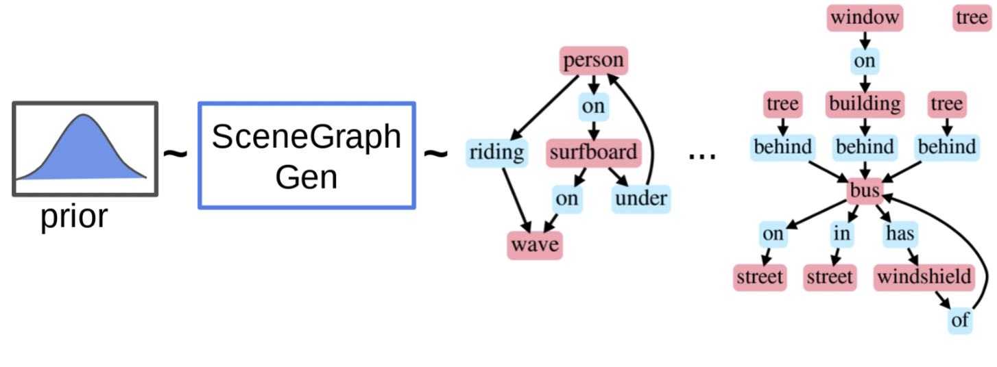
Figure 1: Unconditional Scene Graph Generation

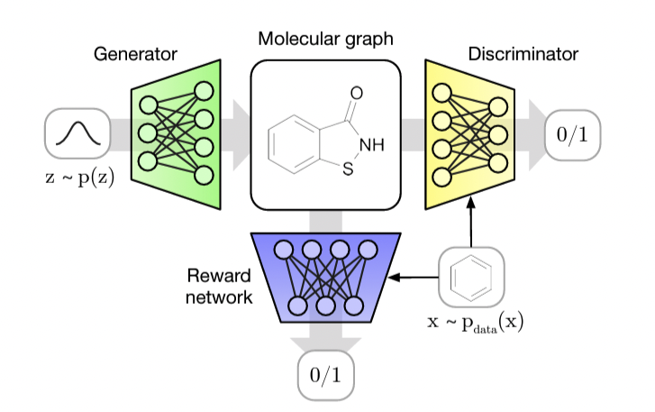
Figure 2: MolGAN model schematics

Unconditional graph generation is the task of generating graphs without any pre-specified constraints or conditions. These methods can be deterministic or can instead learn to sample from a distribution. This task has numerous applications in various fields such as social network analysis, chemical structure design, and image processing. In recent years, deep learning-based models have shown promising results in generating unconditional graphs (Garg et al., 2021; Wang et al., 2019; Kar et al., 2019). Figure 2 shows the schematics for an unconditional scene graph generation model.

Discovering chemical compounds that possess specific characteristics can be a demanding endeavor with significant practical uses, such as creating novel pharmaceuticals from scratch. Likelihood-based methods (Li et al., 2018; Simonovsky and Komodakis, 2018) for generating molecular graphs necessitate either a predetermined (or randomly selected) sequential depiction of the graph or a costly graph matching process to determine the probability of a generated molecule. This is because assessing the likelihood of all feasible node orderings is impractical, even for small-sized graphs. One of the most significant and recent work in this area has been in correspondence to MolGAN (De Cao and Kipf, 2018). MolGAN is an implicit, likelihood free generative model for small molecular graphs that circumvents the need for expensive graph matching procedures or node ordering heuristics of previous likelihood-based methods. The schematic of MolGAN can be found in Figure 2. Some other notable works on chemical compound discovery are Gómez-Bombarelli et al. (2018); Kusner et al. (2017); Dai et al. (2018).

On the contrary, most methods in conditional generation have been on producing a deterministic output. Scene graph generation with image and/or caption supervision is a particularly interesting research topic in this domain (Zhong et al., 2021). There have also been works on road network extraction with image conditioning (Belli and Kipf, 2019). An open source work, called GraphGPT, which generates knowledge graphs from a given text using appropriate prompting on GPT models has also became popular.

Language Models such as BERT (Devlin et al., 2018) and RoBERTa (Liu et al., 2019) have become one of the most widely used models in the field of NLP, and have been applied to a wide range of tasks including question answering (Widad et al., 2022), sentiment analysis (Hoang et al., 2019; Li et al., 2019), and language translation (Zhu et al., 2020; Yang et al., 2020). GPT-3.5, a language model developed by OpenAI, has proven to be a valuable tool for multiple applications (Biswas, 2023; Sallam et al., 2023). However, its applicability in processing or generating graphical data is yet to be fully tested. In this report, we provide the first test of GPT-3.5’s skills in this regard. Rewards have been highly used in Reinforcement Learning. Recently, they have been incorporated in GANs (Zheng et al., 2021; Chen et al., 2022; Xia et al., 2020) for stronger generalization and robustness.

2 Proposed Methods

In this section, we briefly describe the two methods we employed for graph generation. We initially talk about the GPT-3.5 baseline, where we use prompt the GPT-3.5 model to generate graphs based on a description. We then talk about our main contribution of the report: LIC-GAN. We briefly talk about its architecture and some provide some details as to how it was trained.

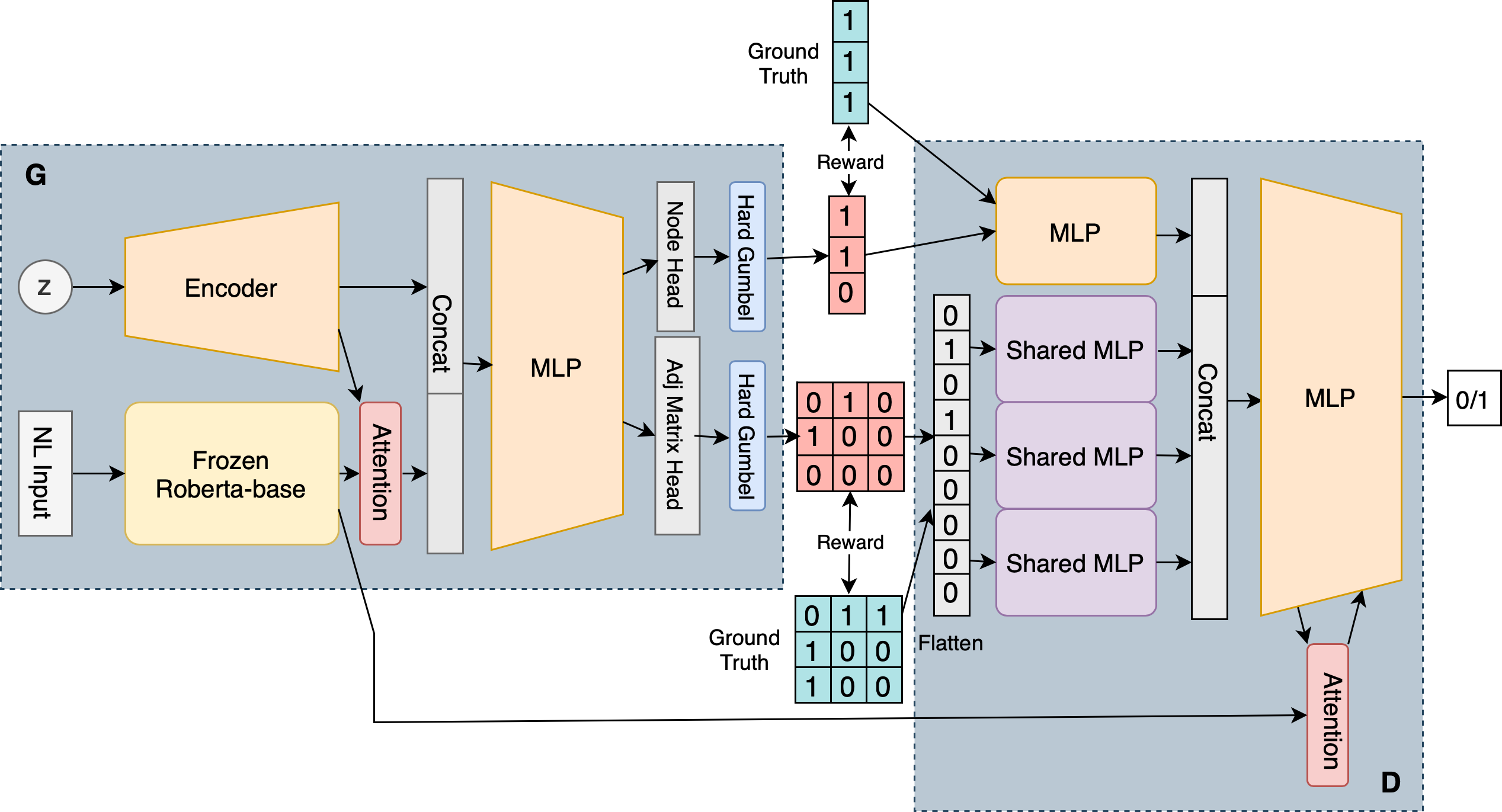
Figure 3: Proposed architecture for natural language conditioned GAN for graph generation

2.1 GPT-3.5 Baseline

Since, there has been no prior work, that has specifically tried to solve the problem of Natural Language Conditioned Graph Generation, we proposed a baseline method using GPT-3.5.

Within the prompt given to GPT-3.5, we define what each of the 5 additional proposed properties mean in the graph-generation context. Furthermore, we also give it some example inputs and outputs.

GPT-3.5 is a chatbot provided by OpenAI, which supports dialogue-like text completion. We designed a simple prompt that ask GPT-3.5 to generate the adjacency matrix. Since the adjacency matrices it generates are sometimes not perfect, we apply a simple post-process that pad the matrix and make it symmetric. The prompt, configuration and the post-processing method is given in A.1.

2.2 LIC-GAN

Model Architecture

The architecture of the final proposed model is shown in Figure 3. The initial models we used for preliminary analysis and architectural decisions had the adjacency matrix alone predicted, from which we obtain the nodes as the rows with all zeros in the matrix. This was later replaced to have two separate prediction heads for the node and edges, which lead to better performance and supported isolated vertices. As opposed to MolGAN’s choice of graph convolutional network (GCN) for the discriminator, we adopt a a weight-shared fully connected network (FCN) to process each row of the adjacency matrix to enforce the symmetry of the node processing (considering the nature of task).

Training Details

WGANs are known to minimize an approximation of the Wasserstein-1 distance. The Wasserstein distance between two distributions $p$ and $q$ can be written as

$$D_{W}[p||q]=\frac{1}{K}\sup_{||f||_{L}\leq K}\left[\mathbb{E}_{x\sim p(x)}[f(x)]-\mathbb{E}_{x\sim q(x)}[f(x)]\right]$$

where supremum is taken from the set of all $K$-Lipschitz functions. We use the WGAN-GP loss formulation used by MolGAN (De Cao and Kipf, 2018) as well for training the model, to improve stability. Similar to the MolGAN model, we also retain the gradient penalty from Gulrajani et al. (2017) scaled by factor $\lambda_{\text{gp}}=5$. For incorporating additional signals to train the GAN, we provide a reward in the form of negative of mean squared loss over node and edge number match. This loss is included in the overall loss after scaling by a factor $\lambda_{\text{rew}}$.

For the preliminary analysis, we use a two hidden-layer FCN to predict the number of nodes from the adjacency matrix in a differentiable manner. For the final model, this becomes unnecessary due to separate dedicated heads.

3 Results

In this section we discuss the results of our model. We initially describe the synthetic datasets that we used in our experiments in section 3.1 and how we evaluate the results of the generative methods in section 3.2. The results of the methods mentioned in the previous section are shown in section 3.3 and 3.5.

3.1 Dataset

To better analyze and benchmark our model, we create a synthetic graph dataset with natural language description of the properties. We utilized NetworkX (Hagberg et al., 2008) to generate four different types of undirected simple graphs (which corresponds to four different graph generation methods).

We consider two datasets: a simple dataset and a complex dataset, for better understanding of how our models are performing. The simple dataset only consists of the number of nodes and the number of edges in the graph in the textual description. Whereas the complex dataset consists of the number of nodes and the number of edges as well as a random subset of the 5 properties listed here: (a) Diam: the diameter (b) Cycle: whether there exists a cycle or not (c) MaxDeg: maximum degree (d) MinDeg: minimum degree (e) CCNum: the number of connected components.

To make the dataset more versatile, we shuffle the properties in the description (for the model to not skip the language inputs and learn simpler correlations) in an online fashion for training all our final baselines and methods. The summary statistics for both datasets can be found in the Appendix B. For a fair comparision between different methods, we generated seperate datasets - train, dev and test, where we use only the test dataset to evaluate the performance all the methods presented in this report. The size of train, dev and test set is $100,000$, $10,000$ and $500$.

3.2 Evaluation

We primarily consider two metrics closeness and property match. They are defined as follows

$${\mathsf{PropMatch}} =\frac{1}{N}\sum_{i=1}^{N}\left(\frac{\sum_{p\in\mathsf{P_{i}}}\mathbbm{1}\left[p(G_{\mathsf{predicted}})=p(G_{\mathsf{true}})\right]}{|P_{i}|}\right)$$

$${\mathsf{Closeness}} =\frac{1}{N}\sum_{i=1}^{N}\left(\frac{\sum_{p\in\mathsf{P_{i}}}\exp\left(-\left(p(G_{\mathsf{predicted}})-p(G_{\mathsf{true}})\right)^{2}\right)}{|P_{i}|}\right)$$

Here $N$ is the number of data points that we are evaluating and $P_{i}$ is the set of properties that are present in the description of the $i^{\mathsf{th}}$ datapoint. It is clear to see that the ${\mathsf{PropMatch}}\leq{\mathsf{Closeness}}$, and that ${\mathsf{PropMatch}}$ is only high if there is a perfect match where as ${\mathsf{Closeness}}$ is a bit forgiving to graphs that have properties that are close enough to the description. We also note that both metrics are going to lie in the $[0,1]$ range.

3.3 GPT-3.5 Results

A brief summary of the results of the method described in Section 2.1 can be found Table 1. The detailed results can be found in Tables 9 and 10 in the Appendix. As can be seen from the results as we make the input more complex (increase the value of $n$), the property match and the closeness both start falling for the simple and the complex dataset. As expected, we can also observe that the complex dataset has significantly lower values of node ${\mathsf{PropMatch}}$ and edge ${\mathsf{PropMatch}}$ as can be seen from Tables 9 and 10. Particularly we note that the node ${\mathsf{PropMatch}}$ went from $0.969$ to $0.178$ for the simple dataset as we transitioned from $n\in[11,25]$ to $n\in[26,50]$. Similarly it dipped from $0.9$ to $0.139$ for the complex dataset. This seems to imply that this method is unlikely to scale for larger graphs.

Dataset	Metric	Overall	$n\in[1,5]$	$n\in[6,10]$	$n\in[11,25]$	$n\in[26,50]$
Simple	${\mathsf{PropMatch}}$	0.423	0.933	0.635	0.522	0.097
	${\mathsf{Closeness}}$	0.468	0.958	0.697	0.542	0.154
Complex	${\mathsf{PropMatch}}$	0.397	0.528	0.514	0.462	0.233
	${\mathsf{Closeness}}$	0.415	0.610	0.564	0.458	0.237

Table 1: GPT-3.5 Performace on the Simple and Complex Dataset. We have split the dataset into 4 buckets based on the graph complexity and show the results across these buckets in the last 4 columns

3.4 LIC-GAN Preliminary Analysis

We initially trained our model for $50$ epochs on the simple dataset (without shuffling the properties) to validate our design choices, and hyperparameters. We describe some of the important design choices based on the results found in Table 2.

• Hard Gumbel Sigmoid vs Sigmoid as output-activation: We found that using Sigmoid to convert logits to adjacency make the convergence of training harder. Therefore, we decide to use Hard Gumbel Sigmoid, an extension of the Gumbel Softmax (Jang et al., 2016)

• Multi-Head Attention vs [CLS] token embedding in generator: Multi-Head Attention allows the generator to access the whole embedding of the description, as opposed to [CLS] token embedding only allows the generator to access the first token embedding. While it is common to represent the whole input with [CLS] token embedding, we found that in our case using Multi-Head Attention gives us a more balanced ${\mathsf{PropMatch}}$ performance.

• RoBERTa vs BERT in generator: We found that the performance for BERT and RoBERTa is similar on our dataset. However, we decide to use RoBERTa because it has a better pretrain performance which might be helpful when the datasett is contains more complex natural language description (the text description in our dataset contains only simple words such as “graph”, “node” and “edge”).

• FCN (Fully Connected Network) vs GCN (Graph Convolution Network) in discriminator: We decide to use FCN instead of GCN because the former gives us a better performance.

• Adjacency matrix only vs Adjacency matrix and node numbers: We found that generating only adjacency matrix and use heuristic to get the number of nodes give us poor performance compared to GPT-3.5. To mitigate this and to support isolated vertices (e.g. vertex with degree $0$), our generator has two output head: a adjacency matrix prediction head and a node prediction head (to indicate the active nodes in the output graph).

We can see that even when we shuffle the positions of the nodes and edges in the description, our model gives a similar performance. Similarly when we use text in the description as opposed to numbers (e.g “two” instead of “2”) we are still able to perform to a similar level. This seems to indicate that the language model is appropriately embedding the information in the description to the feature vector.

$\lambda_{\text{rew}}$	LM	Other Notes	${\mathsf{PropMatch}}$	${\mathsf{Closeness}}$	Node PM	Edge PM
0	BERT		0.2444	0.3287	0.3607	0.1281
0.5	BERT		0.2397	0.3251	0.3578	0.1215
0.5	BERT	Text input	0.2231	0.3235	0.3211	0.1251
0	RoBERTa		0.2437	0.3276	0.3159	0.1235
0	RoBERTa	[CLS] tokens	0.2668	0.3391	0.4587	0.0751
0.5	RoBERTa	[CLS] tokens	0.2405	0.3220	0.3614	0.1196
0.5	RoBERTa	gcns	0.1928	0.2898	0.2676	0.1181
0.5	BERT	Invert $n$ and $m$	0.2228	0.314	0.3397	0.1058
0.5	BERT	Shuffle $n$ and $m$	0.2139	0.3135	0.3007	0.1271
0.5	RoBERTa	[CLS] + Invert $n$ and $m$	0.2241	0.3135	0.3595	0.0887
0.5	RoBERTa	[CLS] + Shuffle $n$ and $m$	0.2244	0.3155	0.3371	0.1117

Table 2: Initial results of LIC-GAN on the simple dataset. LM represents the Language model used on the text description. Node PM and Edge PM represent the property match obtained when we just consider $P_{i}=\{\mathsf{Node}\}$ and $P_{i}=\{\mathsf{Edge}\}$ respectively for all $i=1$ to $N$.

3.5 LIC-GAN Final Results

For our final results, we train the models for $100$ epochs with a constant $2\times 10^{-4}$ learning rate for the generator and discriminator and an Adam optimizer. The results can be found in Table 3, with a more detailed version in Tables 11 and 12 in the Appendix. While the reward helps for the complex dataset (especially for the node and edge match), it does not aid training on the simple dataset as seen in Figures 5 and 5.

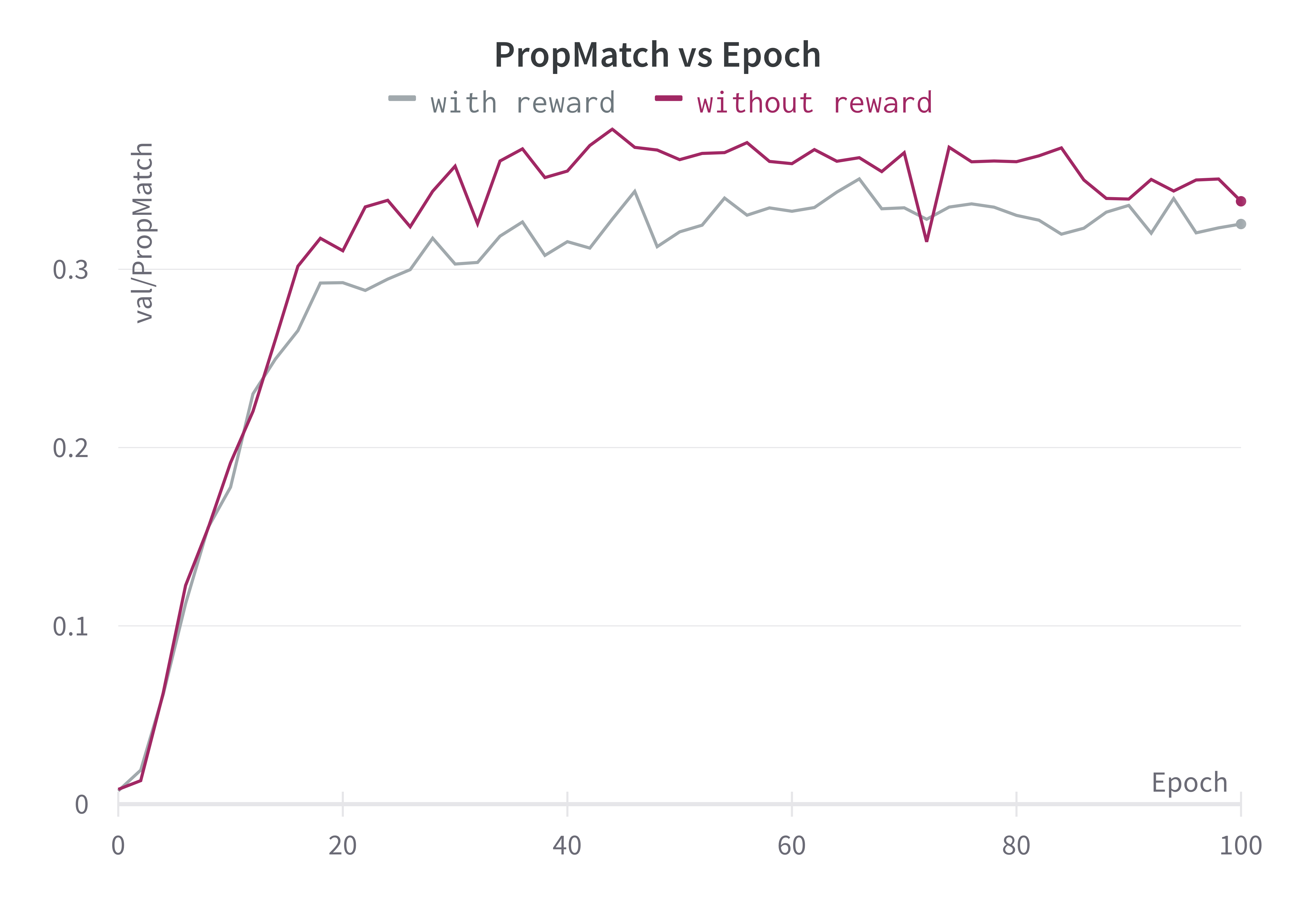
Figure 4: Property Match for final model on simple dataset with $\left(\lambda_{\text{rew}}=0.5\right)$ and without reward

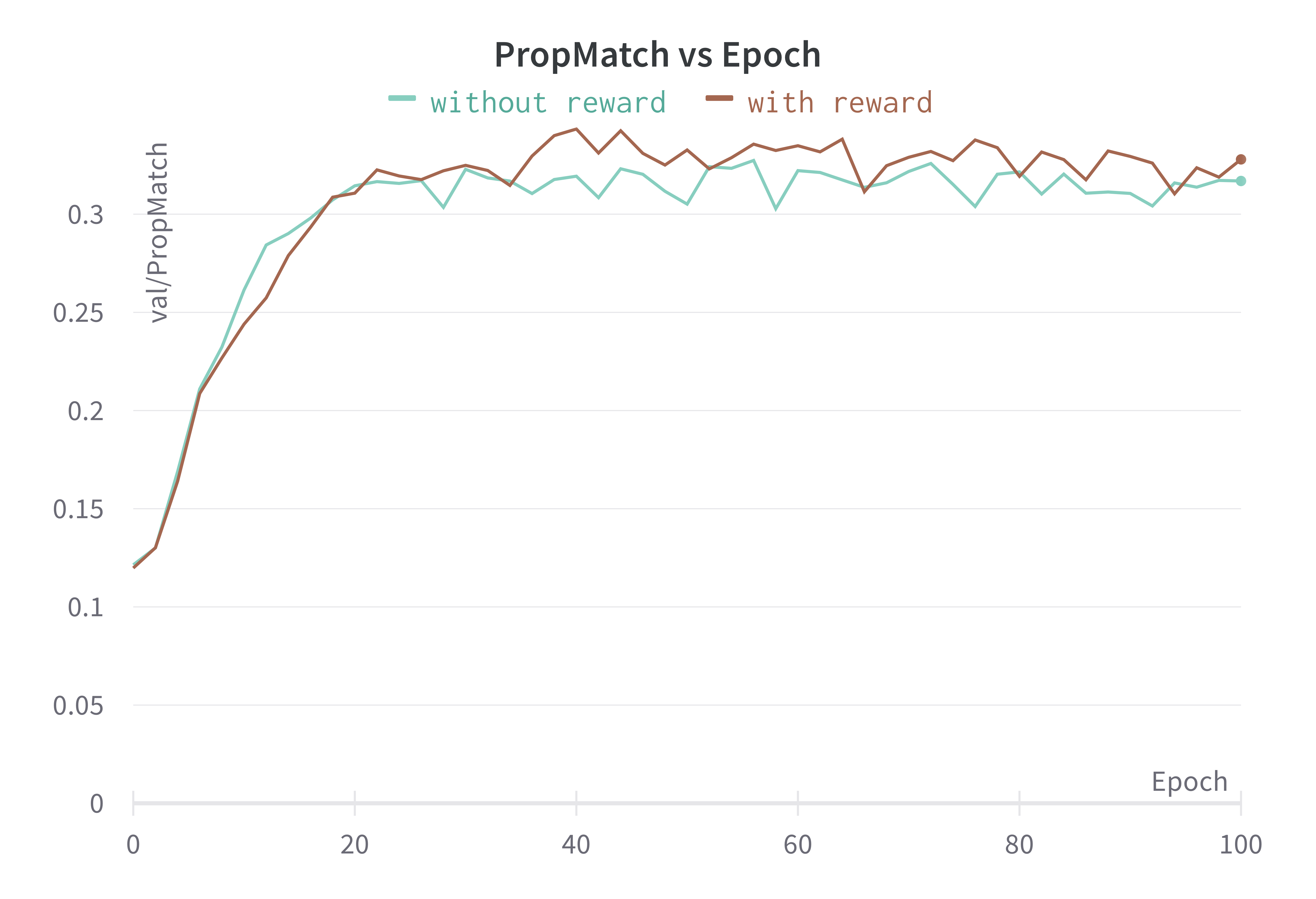
Figure 5: Property Match for final model on complex dataset with $\left(\lambda_{\text{rew}}=0.5\right)$ and without reward

It is observed that, while there is certainly a drop in performance as we increase $n$ for ${\mathsf{PropMatch}}$ and ${\mathsf{Closeness}}$ for both the simple and the complex dataset, the drop is significantly lesser than the one for GPT-3.5. This seems to imply that our LIC-GAN model is likelier to scale for larger graphs unlike the GPT-3.5 model.

Dataset	Metric	Overall	$n\in[1,5]$	$n\in[6,10]$	$n\in[11,25]$	$n\in[26,50]$
Simple	${\mathsf{PropMatch}}$	0.34	0.57	0.45	0.27	0.3
	${\mathsf{Closeness}}$	0.44	0.67	0.54	0.36	0.39
Complex	${\mathsf{PropMatch}}$	0.36	0.47	0.43	0.4	0.26
	${\mathsf{Closeness}}$	0.48	0.62	0.56	0.5	0.39

Table 3: LIC-GAN Performace on the Simple and Complex Dataset. We have split the dataset into 4 buckets based on the graph complexity and show the results across these buckets in the last 4 columns

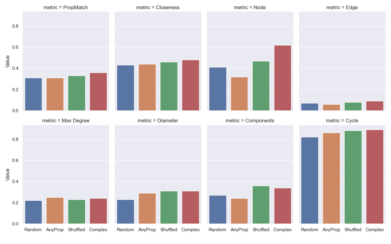
Figure 6: Plots for the performances for some metrics. The 4 experiments are 1) Random: We zero-shot test our trained model on descriptions which do not necessarily contain nodes/edges, 2) AnyProp: We train a new model that does not not necessarily contain nodes/edges in description in during train/test, 3) Shuffled: We zero-shot test descriptions just containing shuffled numeric values 4) Complex: LIC-GAN model’s performance on the test set

4 Discussion and Analysis

In this section, we run two experiments in order to do a ablation study on different parts of our generator e.g. language module and the graph generation module. The shuffled numbers experiments tries to demonstrate that the Language model is extracting crucial information from the textual description. The no node and edge experiments try to show that the graph generation module can generate valid graph even without explicit constraint on graph number and edges.

4.1 The no nodes and edges experiments

Figure 7: The values of the various metrics as we increase the number of properties in the description during the 0-shot learning

We test that the LIC-GAN model was not simply generating a lot of candidate graphs with matching $n$ and $m$ and randomly suggesting graphs that had properties that are close enough. To test our hypothesis, we zero-shot tested a variant of the complex dataset where we randomly choose $2-7$ properties (however, this time we do not compulsorily include nodes and edges in the description). As can be seen from Figure 6 and from Table 13, we perform slightly worse in each metric. Nevertheless we are able to maintain a similar performance which seems to imply that our language model has truly learned the meaning of each of those properties. In fact, this variation of the complex dataset is what one might want to achieve in practice (without having to compulsorily provide any particular property).

However, when we directly train the model on this version of the dataset, we achieve a worse performance compared to the zero-shot evaluation after training on the complex dataset. This validates the importance of implicit (and explicit) reward of preserving one or more easier properties in the description, that guides the training to a better solution.

We also perform another experiment where we zero-shot test a randomly chosen set of properties and progressively increase the number of properties that we choose. The results can be found in Figure 7. These results seem counter-intuitive as for a person if we are just provided a single property is very simple to come up with a graph that satisfies this property as opposed to a description with larger number of properties. However, this likely signals that our model can scale fairly well as we keep increasing the number of properties. The detailed table of results can be found in the Appendix in Table 14.

4.2 The shuffled numbers experiment

We first show that our language model is able to extract information from textual description. We performed the following experiment: for every textual description such as “10 nodes, 20 edges and minimum degree 1” we just gave it the description “20 1 10”, i.e. we removed the property names and shuffled the order of the input sequence. While we expected a significant decrease in performance as we made the task significantly harder, there is not a significant difference in the performance as can be seen from Figure 6. However, we do notice that the biggest performance drop has been in terms of Node’s ${\mathsf{PropMatch}}$. The detailed results for the same can be found in Table 13 in the Appendix.

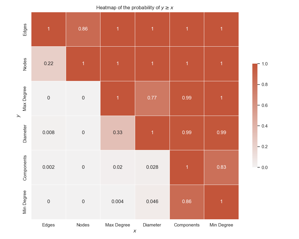
Figure 8: Heatmap showing the probabilities that $y\geq x$

We hypothesize that this is might caused by the fact that Node and Edge are always present (as opposed to the other properties) in the textual description and we have Edge $\geq$ Node int most cases (with the other properties all being less than Node). This allows the model to infer that the maximum number in the property vector is the required number of Edge, and the second largest number is the required number of Node. This explains why the sharpest drop in ${\mathsf{PropMatch}}$ is observed for Node. The heatmap showing the probabilities of ordering of properties can be found in the Appendix in Figure 8. While we observe that there is a similar confusion between MaxDeg and Diam, we believe that there isn’t a significant performance drop here because both of these properties being present in the same description is an unlikely incident in our dataset (probability is around $30\%$). We also note that the most common ordering (Edge $\geq$ Node $\geq$ MaxDeg $\geq$ Diam $\geq$ CCNum $\geq$ MinDeg) appears around $\sim 60\%$ of the time in our dataset.

5 Conclusion

We studied the generation of Natural-Language Conditioned Graphs using GANs, however our work raises several open questions. While, we have primarily worked on generating the graph given the description, both models (LIC-GAN and GPT-3.5) knew that such a graph always existed. An interesting direction would be to have another model predict whether there exists even a single graph that satisfies all of the properties in the description. An example could be a description of the format “A simple undirected graph with 3 nodes and 8 edges”. In conjunction with our model it can potentially generate a better language-conditioned graph generator.

Another possible extension of our work is to make the dataset harder, such as generating directed graph and related properties, or generating weighted graph that satisfy some complex properties like value of min-cut. We can also make the undirected graph generation task harder by adding more advanced graph-theoretic properties (such as planarity, connectivity etc).

Access to Code

All of the code for the project can be found here.

Appendix A Appendix

A.1 GPT-3.5 Prompts and Post-Processing

Post-Processing method

Suppose that given text description $T$, GPT-3.5 generate matrix $G\in\mathbb{R}^{n\times m}$. Note that $n$ is not necessary $m$, WLOG assume that $n\geq m$. The first step is to convert it to a square matrix by padding zeros, then make it symmetric by adding its transpose to itself. In other words, we pad $G$ to $G^{\prime}\in\mathbb{R}^{n\times n}$ then update $G^{\prime}=G^{\prime T}+G^{\prime}$.

Configuration

Parameter	Value
Endpoint	openai.ChatCompletion.create
model	gpt-3.5-turbo
temperature	0
n	1
max_tokens	min(3500, $g^{2}+g+1$), where $g$ is the number of nodes
top_p	1
frequency_penalty	0.0
presence_penalty	0.0
stop	‘‘‘end

Table 4: GPT-3.5 Configuration

GPT-3.5 Prompts

The prompt we use is given below, and is presented in a dialogue style because GPT-3.5 is a chatbot LLM. TEXT_DESCRIPTION is replaced to the text description of graph that we want to generate now.

⬇

1[

2 {

3 ’role’: ’system’,

4 ’content’: "You are given a task to generate an adjacency matrix of an undirected graph with $n$ nodes and $m$ edges. The graph also need to satisfy several properties, which may includes (1) the min among nodes (2) max degree among nodes (3) number of connected components (4) diameter of graph (5) have cycle or not. Diameter of a graph is the maximum distance between any two nodes. A connected component is a subgraph in which any two nodes are connected to each other by paths, and which is connected to no other nodes in the supergraph. A cycle is a path of length at least 3 that starts and ends at the same node. \n\n The graph may be unconnected, but every node has AT LEAST ONE EDGE. If you don’t know how to generate a graph that satisfy all properties, you can output a graph that at least have the correct number of nodes and edges, and match other properties at your best effort. Output the adjacency matrix of the graph only without any other information."

5 },

6 {

7 ’role’: ’system’,

8 ’name’: ’example_user’,

9 ’content’: ’Undirected graph with 9 nodes, 11 edges, 1 connected component, one or more cycle, min degree 1, max di

10ameter 5, max degree 3.’

11 },

12 {

13 ’role’: ’system’,

14 ’name’: ’example_assistant’,

15 ’content’: ’‘‘‘\n0 1 0 0 1 1 0 0 0\n1 0 0 0 0 0 0 1 1\n0 0 0 1 0 0 0 0 0\n0 0 1 0 0 0 1 0 1\n1 0 0 0 0 1 0 0 0\n1 0 0 0 1 0 0 1 0\n0 0 0 1 0 0 0 0 0\n0 1 0 0 0 1 0 0 1\n0 1 0 1 0 0 0 1 0\n‘‘‘end’

16 },

17 {

18 ’role’: ’user’,

19 ’content’: TEXT_DESCRIPTION

20 }

21]

Appendix B Dataset Generation Process and Summary Statistics

B.1 Generation Process

For each graph type, we first randomly choose one configuration among the four possible configurations. Each configuration has a node set $A_{i}$ associated with it, which represents a contiguous segment of numbers. Then, we sample node uniformly from set $A_{i}$, where $A_{1}=[5,9],A_{2}=[10,24],A_{3}=[25,40],A_{4}=[40,50]$. Finally, we generate the graph with the sampled node and parameters. The configuration is given in table 5. We generate three set of data, namely train, dev, test, with different amount of data. Train set has 100k samples, dev set has 10k and test set has 500.

Graph Type	Count	Parameters
Scale Free Graph	30%	n= $A_{1},A_{2},A_{3},A_{4}$
Erdos-Renyi Graph	30%	(n,p)=($A_{1}$,0.3),($A_{2}$,0.2),($A_{3}$,0.1),($A_{4},0.2$)
Random Geometric Graph	30%	(n,r)=($A_{1}$,0.5),($A_{2}$,0.4),($A_{3}$,0.2),($A_{4}$,0.2)
Uniform Random Tree	10%	n=$A_{1},A_{2},A_{3},A_{4}$

Table 5: Methods, parameters and counts for four different graph type. Scale Free Graph Bollobás et al. [2003] is random graphs whose degree follow power law. Erdos-Renyi Graph Erdös and Rényi [1959] is a random graph where each edge has a fixed probability of being created. Random Geometric Graph Penrose [2003] is generated by first scatter points in a 2-d space, then connect points that are close enough. and Uniform Random Tree. $n$ represents number of nodes. $p$ represents the probability of edge creation. $r$ represents the distance threshold value. Please refer to the documentation of NetworkX for more details.

B.2 Summary Statistics

For the following tables, Node represents number of nodes, Edge represents number of edges, Diam represents the diameter of graph among all connected components, CCNum represents the number of connected components, MaxDeg/ MinDeg represents the maximum node degree / minimum node degree.

Train

	Node	Edge	MinDeg	MaxDeg	Diam	CCNum
mean	22.346	37.906	1.196	8.617	5.481	1.227
std	14.201	29.728	0.551	6.141	3.445	0.645
min	5	3	0	1	2	1
25%	9	12	1	4	4	1
50%	19	32	1	7	4	1
75%	35	56	1	10	6	1
max	50	189	7	42	30	8

Table 6: Descriptive Statistics for train set. The size of train set is 100,000.

Dev

	Node	Edge	MinDeg	MaxDeg	Diam	CCNum
mean	22.563	38.307	1.192	8.667	5.471	1.234
std	14.286	30.014	0.556	6.224	3.445	0.649
min	5	3	0	1	2	1
25%	9	12	1	4	4	1
50%	20	32	1	7	4	1
75%	35	56	1	10	6	1
max	50	178	6	40	29	7

Table 7: Descriptive Statistics for dev set. The size of train set is 10,000.

Test

	Node	Edge	MinDeg	MaxDeg	Diam	CCNum
mean	22.446	38.312	1.240	8.622	5.533	1.244
std	14.330	30.418	0.622	5.894	3.776	0.720
min	5	3	0	1	2	1
25%	9	11	1	4	3	1
50%	20	32	1	7	4	1
75%	35	57	1	10	6	1
max	50	155	6	40	26	7

Table 8: Descriptive Statistics for test set. The size of train set is 500.

Property Ordering

Appendix C Detailed Results for GPT-3.5 and LIC-GAN

	Overall	$n\in[1,5]$	$n\in[6,10]$	$n\in[11,25]$	$n\in[25,50]$
${\mathsf{PropMatch}}$	0.423	0.933	0.635	0.522	0.097
${\mathsf{Closeness}}$	0.468	0.958	0.697	0.542	0.154
Node ${\mathsf{PropMatch}}$	0.690	1.000	0.985	0.969	0.178
Edge ${\mathsf{PropMatch}}$	0.156	0.867	0.285	0.075	0.017

Table 9: GPT-3.5 Performace on the Simple Dataset

	Overall	$n\in[1,5]$	$n\in[6,10]$	$n\in[11,25]$	$n\in[25,50]$
${\mathsf{PropMatch}}$	0.397	0.528	0.514	0.462	0.233
${\mathsf{Closeness}}$	0.415	0.610	0.564	0.458	0.237
Node ${\mathsf{PropMatch}}$	0.626	0.867	0.908	0.900	0.139
Edge ${\mathsf{PropMatch}}$	0.058	0.233	0.085	0.044	0.022
MinDeg ${\mathsf{PropMatch}}$	0.266	0.250	0.212	0.367	0.218
MaxDeg ${\mathsf{PropMatch}}$	0.153	0.524	0.344	0.070	0.031
Diam ${\mathsf{PropMatch}}$	0.130	0.353	0.319	0.094	0.000
CCNum ${\mathsf{PropMatch}}$	0.793	0.895	0.828	0.855	0.691
Cycle ${\mathsf{PropMatch}}$	0.814	0.778	0.874	0.852	0.740

Table 10: GPT-3.5 Performace on the Complex Dataset. Diam represents the maximum diameter of the graph. CCNum represnts the number of connected components and Cycle represents whether a graph has a cycle.

	Overall	$n\in[1,5]$	$n\in[6,10]$	$n\in[11,25]$	$n\in[25,50]$
${\mathsf{PropMatch}}$	0.34	0.57	0.45	0.27	0.3
${\mathsf{Closeness}}$	0.44	0.67	0.54	0.36	0.39
Node ${\mathsf{PropMatch}}$	0.59	0.83	0.73	0.5	0.53
Edge ${\mathsf{PropMatch}}$	0.1	0.3	0.16	0.04	0.08

Table 11: LIC-GAN Performace on the Simple Dataset

	Overall	$n\in[1,5]$	$n\in[6,10]$	$n\in[11,25]$	$n\in[25,50]$
${\mathsf{PropMatch}}$	0.36	0.47	0.43	0.4	0.26
${\mathsf{Closeness}}$	0.48	0.62	0.56	0.5	0.39
Node ${\mathsf{PropMatch}}$	0.62	0.9	0.78	0.62	0.46
Edge ${\mathsf{PropMatch}}$	0.09	0.3	0.17	0.06	0.02
MinDeg ${\mathsf{PropMatch}}$	0.02	0.04	0	0	0.05
MaxDeg ${\mathsf{PropMatch}}$	0.24	0.33	0.3	0.26	0.16
Diam ${\mathsf{PropMatch}}$	0.31	0.47	0.4	0.35	0.19
CCNum ${\mathsf{PropMatch}}$	0.34	0.47	0.41	0.52	0.11
Cycle ${\mathsf{PropMatch}}$	0.89	0.83	0.9	0.92	0.87

Table 12: LIC-GAN Performace on the Complex Dataset. Diam represents the maximum diameter of the graph. CCNum represnts the number of connected components and Cycle represents whether a graph has a cycle.

	PM	${\mathsf{Closeness}}$	Node	Edge	MinDeg	MaxDeg	Diam	CCNum	Cycle
Shuffled	0.33	0.46	0.47	0.08	0.02	0.23	0.31	0.36	0.88
Random	0.31	0.43	0.41	0.07	0.01	0.22	0.23	0.27	0.82
Complex	0.36	0.48	0.62	0.09	0.02	0.24	0.31	0.34	0.89

Table 13: PM represents ${\mathsf{PropMatch}}$, for the other properties we represent their ${\mathsf{PropMatch}}$ values. The random dataset was zero-shot tested on the trained model. The random dataset does not necessarily have the number of nodes and edges in the description, whereas the complex dataset always has the nodes and edges in the description. The shuffled dataset just has the shuffled numeric values with the textual description.

Props	PM	${\mathsf{Closeness}}$	Node	Edge	MinDeg	MaxDeg	Diam	CCNum	Cycle
1	0.26	0.35	0.09	0	0.02	0.14	0.01	0	0.88
2	0.27	0.37	0.2	0.02	0.01	0.14	0.14	0.07	0.71
3	0.27	0.39	0.25	0.04	0.01	0.19	0.17	0.1	0.73
4	0.29	0.41	0.36	0.04	0.01	0.23	0.16	0.16	0.78
5	0.32	0.44	0.46	0.06	0.01	0.24	0.24	0.22	0.81
6	0.33	0.46	0.52	0.07	0.01	0.21	0.28	0.27	0.86
7	0.36	0.49	0.63	0.11	0.01	0.26	0.33	0.33	0.86

Table 14: PM represents ${\mathsf{PropMatch}}$, for the other properties we represent their ${\mathsf{PropMatch}}$ values, while Props represents the number of properties used for performing zero-shot testing

References

- Belli and Kipf (2019) D. Belli and T. Kipf. Image-conditioned graph generation for road network extraction, 2019.
- Biswas (2023) S. S. Biswas. Potential use of chat gpt in global warming. Annals of biomedical engineering, pages 1–2, 2023.
- Bollobás et al. (2003) B. Bollobás, C. Borgs, J. T. Chayes, and O. Riordan. Directed scale-free graphs. In ACM-SIAM Symposium on Discrete Algorithms, 2003.
- Bronstein et al. (2017) M. M. Bronstein, J. Bruna, Y. LeCun, A. Szlam, and P. Vandergheynst. Geometric deep learning: Going beyond euclidean data. IEEE Signal Processing Magazine, 34(4):18–42, 2017. doi: 10.1109/MSP.2017.2693418.
- Chen et al. (2022) X. Chen, L. Yao, X. Wang, A. Sun, and Q. Z. Sheng. Generative adversarial reward learning for generalized behavior tendency inference. IEEE Transactions on Knowledge and Data Engineering, pages 1–12, 2022. doi: 10.1109/TKDE.2022.3186920.
- Dai et al. (2018) H. Dai, Y. Tian, B. Dai, S. Skiena, and L. Song. Syntax-directed variational autoencoder for molecule generation. In Proceedings of the international conference on learning representations, 2018.
- De Cao and Kipf (2018) N. De Cao and T. Kipf. MolGAN: An implicit generative model for small molecular graphs. ICML 2018 workshop on Theoretical Foundations and Applications of Deep Generative Models, 2018.
- Devlin et al. (2018) J. Devlin, M.-W. Chang, K. Lee, and K. Toutanova. Bert: Pre-training of deep bidirectional transformers for language understanding. arXiv preprint arXiv:1810.04805, 2018.
- Erdös and Rényi (1959) P. Erdös and A. Rényi. On random graphs i. Publicationes Mathematicae Debrecen, 6:290–297, 1959.
- Garg et al. (2021) S. Garg, H. Dhamo, A. Farshad, S. Musatian, N. Navab, and F. Tombari. Unconditional scene graph generation. In Proceedings of the IEEE/CVF International Conference on Computer Vision, pages 16362–16371, 2021.
- Gómez-Bombarelli et al. (2018) R. Gómez-Bombarelli, J. N. Wei, D. Duvenaud, J. M. Hernández-Lobato, B. Sánchez-Lengeling, D. Sheberla, J. Aguilera-Iparraguirre, T. D. Hirzel, R. P. Adams, and A. Aspuru-Guzik. Automatic chemical design using a data-driven continuous representation of molecules. ACS Central Science, 4(2):268–276, Feb 2018. ISSN 2374-7943. doi: 10.1021/acscentsci.7b00572. URL https://doi.org/10.1021/acscentsci.7b00572.
- Gulrajani et al. (2017) I. Gulrajani, F. Ahmed, M. Arjovsky, V. Dumoulin, and A. C. Courville. Improved training of wasserstein gans. Advances in neural information processing systems, 30, 2017.
- Hagberg et al. (2008) A. A. Hagberg, D. A. Schult, and P. J. Swart. Exploring network structure, dynamics, and function using networkx. In G. Varoquaux, T. Vaught, and J. Millman, editors, Proceedings of the 7th Python in Science Conference, pages 11 – 15, Pasadena, CA USA, 2008.
- Hamilton et al. (2017) W. L. Hamilton, R. Ying, and J. Leskovec. Representation learning on graphs: Methods and applications. CoRR, abs/1709.05584, 2017. URL http://arxiv.org/abs/1709.05584.
- Hoang et al. (2019) M. Hoang, O. A. Bihorac, and J. Rouces. Aspect-based sentiment analysis using BERT. In Proceedings of the 22nd Nordic Conference on Computational Linguistics, pages 187–196, Turku, Finland, Sept.–Oct. 2019. Linköping University Electronic Press. URL https://aclanthology.org/W19-6120.
- Jang et al. (2016) E. Jang, S. Gu, and B. Poole. Categorical reparameterization with gumbel-softmax. arXiv preprint arXiv:1611.01144, 2016.
- Kar et al. (2019) A. Kar, A. Prakash, M.-Y. Liu, E. Cameracci, J. Yuan, M. Rusiniak, D. Acuna, A. Torralba, and S. Fidler. Meta-sim: Learning to generate synthetic datasets. In ICCV, 2019.
- Khoshraftar and An (2022) S. Khoshraftar and A. An. A survey on graph representation learning methods. arXiv preprint arXiv:2204.01855, 2022.
- Kusner et al. (2017) M. J. Kusner, B. Paige, and J. M. Hernández-Lobato. Grammar variational autoencoder. In D. Precup and Y. W. Teh, editors, Proceedings of the 34th International Conference on Machine Learning, volume 70 of Proceedings of Machine Learning Research, pages 1945–1954. PMLR, 06–11 Aug 2017. URL https://proceedings.mlr.press/v70/kusner17a.html.
- Li et al. (2019) X. Li, L. Bing, W. Zhang, and W. Lam. Exploiting bert for end-to-end aspect-based sentiment analysis. arXiv preprint arXiv:1910.00883, 2019.
- Li et al. (2018) Y. Li, O. Vinyals, C. Dyer, R. Pascanu, and P. Battaglia. Learning deep generative models of graphs. arXiv preprint arXiv:1803.03324, 2018.
- Liu et al. (2019) Y. Liu, M. Ott, N. Goyal, J. Du, M. Joshi, D. Chen, O. Levy, M. Lewis, L. Zettlemoyer, and V. Stoyanov. Roberta: A robustly optimized bert pretraining approach. arXiv preprint arXiv:1907.11692, 2019.
- Penrose (2003) M. Penrose. Random geometric graphs, volume 5. OUP Oxford, 2003.
- Sallam et al. (2023) M. Sallam, N. Salim, M. Barakat, and A. Al-Tammemi. Chatgpt applications in medical, dental, pharmacy, and public health education: A descriptive study highlighting the advantages and limitations. Narra J, 3(1):e103–e103, 2023.
- Simonovsky and Komodakis (2018) M. Simonovsky and N. Komodakis. Graphvae: Towards generation of small graphs using variational autoencoders. In Artificial Neural Networks and Machine Learning–ICANN 2018: 27th International Conference on Artificial Neural Networks, Rhodes, Greece, October 4-7, 2018, Proceedings, Part I 27, pages 412–422. Springer, 2018.
- Wang et al. (2019) K. Wang, Y.-A. Lin, B. Weissmann, M. Savva, A. X. Chang, and D. Ritchie. Planit: Planning and instantiating indoor scenes with relation graph and spatial prior networks. ACM Trans. Graph., 38(4), jul 2019. ISSN 0730-0301. doi: 10.1145/3306346.3322941. URL https://doi.org/10.1145/3306346.3322941.
- Widad et al. (2022) A. Widad, B. L. El Habib, and E. F. Ayoub. Bert for question answering applied on covid-19. Procedia Computer Science, 198:379–384, 2022. ISSN 1877-0509. doi: https://doi.org/10.1016/j.procs.2021.12.257. URL https://www.sciencedirect.com/science/article/pii/S1877050921024960. 12th International Conference on Emerging Ubiquitous Systems and Pervasive Networks / 11th International Conference on Current and Future Trends of Information and Communication Technologies in Healthcare.
- Xia et al. (2020) Y. Xia, J. Zhou, Z. Shi, C. Lu, and H. Huang. Generative adversarial regularized mutual information policy gradient framework for automatic diagnosis. Proceedings of the AAAI Conference on Artificial Intelligence, 34(01):1062–1069, Apr. 2020. doi: 10.1609/aaai.v34i01.5456. URL https://ojs.aaai.org/index.php/AAAI/article/view/5456.
- Yang et al. (2020) J. Yang, M. Wang, H. Zhou, C. Zhao, W. Zhang, Y. Yu, and L. Li. Towards making the most of bert in neural machine translation. In Proceedings of the AAAI conference on artificial intelligence, volume 34, pages 9378–9385, 2020.
- Zheng et al. (2021) C. Zheng, S. Yang, J. Parra-Ullauri, A. Garcia-Dominguez, and N. Bencomo. Reward-reinforced reinforcement learning for multi-agent systems. arXiv preprint arXiv:2103.12192, 2021.
- Zhong et al. (2021) Y. Zhong, J. Shi, J. Yang, C. Xu, and Y. Li. Learning to generate scene graph from natural language supervision, 2021.
- Zhu et al. (2020) J. Zhu, Y. Xia, L. Wu, D. He, T. Qin, W. Zhou, H. Li, and T.-Y. Liu. Incorporating bert into neural machine translation. arXiv preprint arXiv:2002.06823, 2020.