Field equation of thermodynamic gravity and galactic rotational curves

Abstract.

The rotational velocity curve (RC) of galaxy NGC 3198 is modelled in various theoretical frameworks: Thermodynamic Gravity (TG) is compared to Dark Matter (DM) and Modified Newtonian Dynamics (MOND). The nonlinear gravitational field equation of TG is solved using the baryonic mass density as the source of the gravitational field. In this paper, first a dissipation motivated numerical method is verified with the help of exact solutions. Then, the obtained optimal velocity curve is compared to pseudo-isothermal DM and MOND parametrisations for the RC of the galaxy.

1. Introduction

The most successful model in cosmology so far is the so-called $\Lambda$CDM model, where $\Lambda$ stands for the cosmological constant in the Einstein-equation accounting for dark energy, and CDM stands for cold dark matter. The composition of DM is unknown. There is an ongoing theoretical, experimental and computational hunt to find proper candidates in the framework of existing or new particles of the Standard Model of Particle Physics [1, 2, 3].

The most well-known effect of dark matter is its influence on the rotation curves of galaxies. Properly modelling the observed galactic rotational velocity curves with DM requires particular dark matter distributions, [4, 1]. However, in spite of the flexibility in modelling with the help of a potentially unknown distribution, there are some well-known problems and inconsistencies both in the case of individual galaxies and general, global properties.

Regularities in baryon-DM coupling can be summarised in the Radial Acceleration Relation (RAR). This relation generalises the more well-known dynamical relations, like Renzo’s rule or the baryonic Tully-Fisher relation. The RAR encompasses these effects for various types of galaxies and establishes the strong connection between the baryonic contribution and the rotation curve [5, 6]. These regularities indicate that DM is not a simple passive background but interacts with the baryonic mass component.

Related well-documented problems of the $\Lambda$CDM paradigm are the core-cusp problem, the missing satellite problem and the too-big-to-fail problem. The simulations that include dark matter predict that DM halo density profiles should rise steeply at small radii as $\rho(r)\propto r^{-\gamma}$ with $\gamma\simeq 0.8-1.4$ for small galaxies. This is in contrast to observations with many low-mass DM-dominated galaxies. A related ’central density problem’ also exists as simulations predict more dark matter in the central regions than they should host. These two issues (low-density cores and high-density cusps) are summarised as the core-cusp problem [7]. That is one of the reasons that the hydrodynamics-motivated pseudo-isothermal (ISO) DM distribution is widely used for rotational velocity curve modelling.

Because of the above-mentioned problematic aspects, there are several other proposals to explain the missing mass. The superfluid theories suggest a particular multi-component form of dark matter, [8, 9, 10], where the explanation of rotational curves may come from a logarithmic field potential, [11, 12], or scale invariance, [13].

Among these suggestions, the most popular and most developed is MOND. Its success is based on the insight regarding the nonrelativistic, phenomenological observations, in particular, the galactic rotational curves. The reason became clear after the development of the first modified gravity version of MOND, called A QUAdratic Lagrangian theory (AQUAL), [14]. It has a vacuum solution with a force that is inversely proportional to the distance of the central mass: that can exactly counterbalance the centrifugal force and explain the typical flat velocity profiles.

While MOND has remarkable success in explaining many observational features of the local Universe [15], and TeVeS, the relativistic extension of AQUAL, is successful in explaining gravitational lensing and matter perturbation evolution, as Dodelson [16] points out, it still faces serious challenges, notably in the explanation of galaxy clusters, and the shape of the power spectrum of baryon-acoustic oscillations.

A different approach was proposed by Verlinde, whose emergent gravity (also known as entropic gravity) uses the idea that spacetime and gravity emerge together from the entanglement structure of an underlying microscopic theory. Using insights from black hole thermodynamics, quantum information theory and string theory, emergent gravity is motivated and borrows elements of various nonrelativistic constitutive theories. For the DM phenomena, emergent gravity is motivated by generalised nonrelativistic elasticity [17]. The AQUAL type field equation in the nonrelativistic limit can be obtained from a covariant version of the theory, [18].

There is also a theory of gravity based on nonequilibrium thermodynamics, refered as thermodynamic gravity (TG) in the following, [19, 20]. Then the gravitational potential is treated as a thermodynamic state variable and the standard Newtonian gravity can be derived. The approach is based on the simple and only assumption that field energy and interaction energy is included in the total energy density. Then the inequality describing the entropy production rate in a local equilibrium state leads to the following dissipative field equation for gravity:

(1) $$\frac{\partial\varphi}{\partial t}=\frac{l^{2}}{\tau}\left(\Delta\varphi-K\left(\nabla\varphi\right)^{2}-4\pi G\rho\right),$$

where $\varphi$ is the gravitational potential field, $l$ refers to the macroscopic spatial scale of variations of the whole system, $\tau$ is the relaxation time, $\Delta$ is the Laplace operator, $K$ is a characteristic coefficient of the dimensions $s^{2}m^{-2}$, $G$ is the Newtonian constant of gravity and $\rho$ is the mass density. The stationary solution yields a nonlinear field equation for a modified gravitational interaction, while the strength of deviation from the classical case is characterised by the $K$ constant, which arises from the linear coupling between the gravitational and mechanical interactions. This leads to a dynamic crossover between Newtonian and non-Newtonian regimes.

There, the relaxation to a stationary nonlinear field equation indicates the dissipative character of the theory. The nonlinear term is due to the presence of the gravitational field pressure, which is a consequence of the holographic properties of Newtonian gravity, and in general, the result of thermodynamic requirements, [21].

Therefore, due to the pressure of the gravitational field, there is a cross effect between the thermodynamic force of the scalar gravitational interaction and the scalar part of the mechanical interaction and the nonlinear term of eq. 1 emerges naturally. Therefore, the parameter $K$ is not fundamental, it belongs to a particular transport property of the thermodynamic cross effect of gravitational field and mechanical momentum transport: the gravitational field transports material momentum and material momentum pulls the related gravity field along. $K$ is a material parameter that characterises the intensity of the aforementioned coupling in a galactic environment, therefore it is not a self-energy term as in the similar field equations of [22, 23, 24]. Also, it has a direct physical interpretation, as $v_{K}=K^{-1/2}$ is a characteristic velocity of a flat rotational curve because $F_{K}=\frac{1}{Kr}$ is the force field in a stationary vacuum solution of the field equation in TG.

In the TG theory, the source term of the field equation is the density distribution of the baryonic mass, the sum of the visible matter and the atomic hydrogen densities. The gravitational field and the corresponding centrifugal force can be calculated by solving the stationary part of eq. 1. This paper serves as a proof of concept for this method, to be detailed for additional galaxies in following publications.

In the following sections, we give a finite difference scheme to solve the field equations and verify the method with the help of known exact solutions of the equation with constant, $\rho_{0}\geq 0$ density distributions. Then, we demonstrate the applicability of the method, solving the equation with a realistic example, with the mass distribution of galaxy NGC 3198 as a source term. Here the sum of the visible part (referenced also as a stellar disk) and the atomic H (HI) component is used to solve the stationary part of the field equation 1. The numerical method is of a relaxational type, exploiting that the time-dependent field equation relaxes to the stationary solution.

The paper first presents the exact solutions of the equation. Then, a short description of the numerical method is given. Afterwards, we validate the method, showing that the numerical scheme relaxes to the known exact solutions. Then, the velocity curve of the NGC 3198 galaxy is modelled, fitting the K parameter. Finally, a short analysis and interpretation follow.

2. Thermodynamic gravity

For the exact and numerical solutions, a spherically symmetric case will be treated, with the $r$ variable denoting the distance from the centre, as before. In this case, equation 1 can be rewritten into the following form:

(2) $$\partial_{t}\varphi=\frac{l^{2}}{\tau}\left(\partial_{rr}\varphi+\frac{2}{r}\partial_{r}\varphi-4\pi G\rho-K(\partial_{r}\varphi)^{2}\right).$$

2.1. Exact solutions

In this section the analytical solution for the stationary part of eq. 1 is investigated in the spherically symmetric case. Let us introduce the following shorthand notation:

(3) $$\partial_{r}\varphi(r)=\varphi^{\prime},$$

(4) $$\partial_{rr}\varphi(r)=\varphi^{\prime\prime}.$$

If the field is time-independent, then $\varphi(\mathbf{r},t)$ can be written for $\varphi(r)$ as

(5) $$\varphi^{\prime\prime}=-\frac{2}{r}\varphi^{\prime}+4\pi G\rho(r)+K\left(\varphi^{\prime}\right)^{2},$$

whereby using gravitational acceleration, which is by definition

(6) $$\mathbf{g}=-\nabla\varphi,$$

and here becomes

(7) $$g(r)=-\varphi^{\prime},$$

we may obtain the following form:

(8) $$g(r)^{\prime}=-\frac{2}{r}g(r)-4\pi G\rho(r)-Kg(r)^{2}.$$

This non-linear Ricatti equation has well-known solutions when the density is zero or a constant value.

2.1.1. Vacuum solution

For solutions with zero density, i.e. $\rho(r)=0$, eq. 8 becomes

(9) $$g(r)^{\prime}=-\frac{2}{r}g(r)-Kg(r)^{2},$$

which is a Bernoulli-type equation, and can be solved by introducing:

(10) $$w(r)=g(r)^{-1},$$

whereupon eq. 9 becomes:

(11) $$w(r)^{\prime}-\frac{2}{r}w=K.$$

This is a first-order linear ordinary differential equation, and has the following solution:

(12) $$w(r)=-Cr^{2}-Kr.$$

By substituting this into eq. 10, one can obtain the following formulas:

(13) $$g(r)=-\frac{1}{Kr+Cr^{2}},$$

(14) $$\varphi(r)=-\frac{1}{K}\ln{\frac{r}{K+Cr}}+\varphi_{0}.$$

This solution has a singularity at $r=0$, so it may only be used after the effect of the mass distribution is negligible (e.g. far from the bulk of the galactic mass). The $C$ constant then may be fitted using the boundary condition at the transition to this regime. One can recover the Newtonian solution with a central point mass, if $K$ tends to zero:

(15) $$-\frac{GM}{r^{2}}=g(r)_{K=0}=-\frac{1}{Cr^{2}},$$

(16) $$C:=\frac{1}{GM_{aa}}.$$

This indicates that the parameter corresponds to an apparent asymptotic equivalent point-mass ($M_{aa}$) at the centre of our field. Therefore, introducing also the characteristic distance, $R=K/C$, one obtains the vacuum solution in the following intuitive form, [20]:

(17) $$g(r)=-\frac{GM_{aa}}{(R+r)r}.$$

2.1.2. Solution with constant density

Eq. 8 can be solved analytically if the density is a nonzero $\rho_{c}$ constant, too. Then a general solution can be written as

(18) $$g(r)=\frac{1}{Kr}+\frac{\sqrt{-4\pi G\rho_{c}K}}{K}\tan\left(\sqrt{-4\pi G\rho_{c}K}\cdot r+C\right).$$

For further consideration, let us examine the cases where $K>0$ and $K<0$. In the $K>0$ case, we can rewrite eq. 18 as

(19) $$g_{+}(r)=\frac{1}{Kr}+\sqrt{\frac{4\pi G\rho_{c}}{K}}\cdot i\tan\left(i\sqrt{4\pi G\rho_{c}K}\cdot r+C\right),$$

(20) $$i\tilde{C}=C,$$

(21) $$g_{+}(r)=\frac{1}{Kr}-\sqrt{\frac{4\pi G\rho_{c}}{K}}\cdot\tanh\left(\sqrt{4\pi G\rho_{c}K}\cdot r+\tilde{C}\right),$$

and in the $K<0$ case, as

(22) $$g_{-}(r)=-\frac{1}{|K|r}-\sqrt{\frac{4\pi G\rho_{c}}{|K|}}\cdot\tan\left(\sqrt{4\pi G\rho_{c}|K|}\cdot r+C\right).$$

Here $i$ is the imaginary unit, $C$ and $\tilde{C}$ are constants. Since for this constant density mass model we want to eliminate the singularity at $r=0$, we may do so by appropriately choosing $C$ or $\tilde{C}$. By choosing $\tilde{C}=i\frac{\pi}{2}$, the $\tanh(x)$ function becomes $\coth(x)$, and will have the following series representation in the equation:

(23) $$g_{+}(r)=\frac{1}{Kr}-\sqrt{\frac{4\pi G\rho_{c}}{K}}\cdot\coth\left(\sqrt{4\pi G\rho_{c}K}\cdot r\right)$$

$$\approx\frac{1}{Kr}-\sqrt{\frac{4\pi G\rho_{c}}{K}}\cdot\left(\frac{1}{\sqrt{4\pi G\rho_{c}K}\cdot r}+\frac{\sqrt{4\pi G\rho_{c}K}\cdot r}{3}-\frac{\left(\sqrt{4\pi G\rho_{c}K}\right)^{3}\cdot r^{3}}{45}+\mathcal{O}\left(r^{5}\right)\right)$$

$$\approx-\frac{1}{3}\cdot 4\pi G\rho_{c}\cdot r+\frac{K}{45}\left(4\pi G\rho_{c}\right)^{2}\cdot r^{3}+\mathcal{O}\left(r^{5}\right),$$

and thus eliminates the singularity. We can note that the first term corresponds to the usual result in the case of Newtonian gravity, while the higher-order terms, which also contain the $K$ parameter, serve as corrections. For $g_{-}(r)$, we can choose $C=\frac{\pi}{2}$ and obtain similarly:

(24) $$g_{-}(r)=-\frac{1}{|K|r}+\sqrt{\frac{4\pi G\rho_{c}}{|K|}}\cdot\cot\left(\sqrt{4\pi G\rho_{c}|K|}\cdot r\right)$$

$$\approx-\frac{1}{|K|r}+\sqrt{\frac{4\pi G\rho_{c}}{|K|}}\cdot\left(\frac{1}{\sqrt{4\pi G\rho_{c}|K|}\cdot r}-\frac{\sqrt{4\pi G\rho_{c}|K|}\cdot r}{3}-\frac{\left(\sqrt{4\pi G\rho_{c}|K|}\right)^{3}\cdot r^{3}}{45}+\mathcal{O}(r^{5})\right)$$

$$\approx-\frac{1}{3}\cdot 4\pi G\rho_{c}\cdot r-\frac{|K|}{45}\left(4\pi G\rho_{c}\right)^{2}\cdot r^{3}+\mathcal{O}\left(r^{5}\right).$$

which is the same in the first two orders as in the previous case, considering the sign of $K$. The difference only appears in terms containing higher orders of $K$, as the two series diverge.

2.2. Numerical solution

This chapter details the numerical method for the solution of eq. 2. Here, generally, $\rho(r,t)$ can be a function of time, as it is coupled to the fundamental hydrodynamic balances. However, changes in the density due to the characteristic speed of matter will be considered negligible relative to the relaxation of the potential. This is justified by experimental boundaries on the possible delay time of the gravitational field, summarised in the work of Diósi [25], and the characteristic timescale must be below millisecond. This insight also serves as a justification to numerically treat the gravitational potential as relaxing to the stationary solution in eq. 2.

2.2.1. Dimensionless formalism

In order to solve the equation, a dimensionless form is created, by introducing the following notation:

(25) $$\rho=\rho_{d}\tilde{\rho},$$

(26) $$\frac{l^{2}}{\tau}=a,$$

(27) $$r=r_{d}\tilde{r},$$

(28) $$\varphi=\varphi_{d}\tilde{\varphi},$$

(29) $$K=\frac{1}{\varphi_{d}}\tilde{K},$$

(30) $$t=t_{d}\tilde{t}\rightarrow t_{d}=\frac{r_{d}^{2}\tau}{l^{2}}=\frac{r_{d}^{2}}{a},$$

where the quantities with the index $d$ denote a value with appropriate dimensions and the values with a tilde are dimensionless. Substituting these into eq. 2, we obtain the following:

(31) $$\frac{\partial\left(\varphi_{d}\tilde{\varphi}\right)}{\partial\left(t_{d}\tilde{t}\right)}=a\left(\frac{\partial^{2}\left(\varphi_{d}\tilde{\varphi}\right)}{\partial\left(r_{d}\tilde{r}\right)^{2}}+\frac{2}{r_{d}\tilde{r}}\frac{\partial\left(\varphi_{d}\tilde{\varphi}\right)}{\partial\left(r_{d}\tilde{r}\right)}-4\pi G\rho_{d}\tilde{\rho}-\frac{1}{\varphi_{d}}\tilde{K}\left(\frac{\partial\left(\varphi_{d}\tilde{\varphi}\right)}{\partial\left(r_{d}\tilde{r}\right)}\right)^{2}\right),$$

(32) $$\frac{\partial\tilde{\varphi}}{\partial\tilde{t}}=\frac{\partial^{2}\tilde{\varphi}}{\partial\tilde{r}^{2}}+\frac{2}{\tilde{r}}\frac{\partial\tilde{\varphi}}{\partial\tilde{r}}-\frac{4\pi G\rho_{d}r_{d}^{2}}{\varphi_{d}}\tilde{\rho}-\tilde{K}\left(\frac{\partial\tilde{\varphi}}{\partial\tilde{r}}\right)^{2}.$$

Let us also choose

(33) $$\frac{4\pi G\rho_{d}r_{d}^{2}}{\varphi_{d}}\overset{!}{=}1.$$

By leaving the tilde notation, we obtain the equation analogue to eq. 2 in the following form:

(34) $$\partial_{t}\varphi=\partial_{rr}\varphi+\frac{2}{r}\partial_{r}\varphi-\rho-K\left(\partial_{r}\varphi\right)^{2}.$$

For the numerical method, $r_{d}$ is chosen to be the furthest point of the velocity curve data and $\rho_{d}$ as the mean of the derived density distribution, as can be seen later in eq. 48.

2.2.2. Discretisation

In order to solve eq. 34 numerically, a discretisation method of staggered grids is employed [26, 27, 28]. This means that the derivative of the field is introduced as $q=\partial_{r}\varphi$, which allows us to rewrite eq. 34 as a system of two first-order differential equations:

(35) $$\partial_{t}\varphi=\partial_{r}q+\frac{2}{r}q-\rho-Kq^{2},$$

(36) $$q=\partial_{r}\varphi.$$

The aim of this method is the numerical prescription of Neumann-type boundary conditions and the better numerical handling of the nonlinear term with the coefficient $K$. During the numerical solution, in a given timestep, the $\varphi$ field is evaluated first, using the values of $\varphi$ and $q$ from the previous timestep, and then the derivate field $q$ is evaluated, using the obtained new field value. In the staggered grids method, the two variables are shifted by $\Delta x/2$ for better handling. The schematic representation of this can be seen in Fig. 1. Henceforth, $r$ will be shown with dimensional values (e.g. $r=r_{d}$ for $\tilde{r}=1$) for easier comprehension, however, all other physical quantities remain dimensionless.

Figure 1. The schematic representation of the discretisation method of staggered grids, which was used in the numerical solution [26]. The (Neumman-type) boundary conditions (B.C.) are set for the derivative field.

For the terms containing $q$ explicitly, the average of the $q$ field at two spatially neighbouring points can be used. By denoting the spatial indices with $j$ and the temporal indices with $t$, the two equations can be simply discretised in the following way:

(37) $$\varphi_{j,t+1}=\varphi_{j,t}+\Delta t\left(\frac{q_{j+1,t}-q_{j,t}}{\Delta x}+\frac{2}{\left(\frac{1}{2}+j\right)\cdot\Delta x}\frac{q_{j,t}+q_{j+1,t}}{2}-\rho_{j}-K\left(\frac{q_{j,t}+q_{j+1,t}}{2}\right)^{2}\right),$$

(38) $$q_{j,t+1}=\frac{\varphi_{j,t+1}-\varphi_{j-1,t+1}}{\Delta x}.$$

In order to ensure the stability of the numerical method, a sufficiently small $\frac{\Delta t}{\Delta x^{2}}$ ratio was chosen. Unless otherwise noted, for the numerical calculations, $N=200$ was used. The initial conditions for the arrays $\varphi$ and $q$ were chosen to be

(39) $$\varphi(t=0)=0,$$

(40) $$q(t=0)=0,$$

except in the boundaries, while the boundary conditions were

(41) $$q(r=0)=0,$$

(42) $$q(r=r_{d})=\frac{v_{observed}(r_{d})^{2}}{\varphi_{d}},$$

during the galaxy velocity curve calculation. For the reliability testing, the boundaries were set to the corresponding values of the theoretical curves.

2.2.3. Convergence and reliability

In order for the numerical solution to yield a good enough approximation of the stationary solution, the number of the timesteps needs to be sufficiently high. To ensure this, the number of temporal iterations $T$ is set to fulfil the following:

(43) $$T\cdot\Delta t=1\rightarrow T=\frac{1}{\Delta t}.$$

The relaxation process is shown for the relaxation of the potential and the derivative in Fig. 2. As can be seen, the method converges fast, and this choice provides enough timesteps for a good convergence to the theoretical solution.

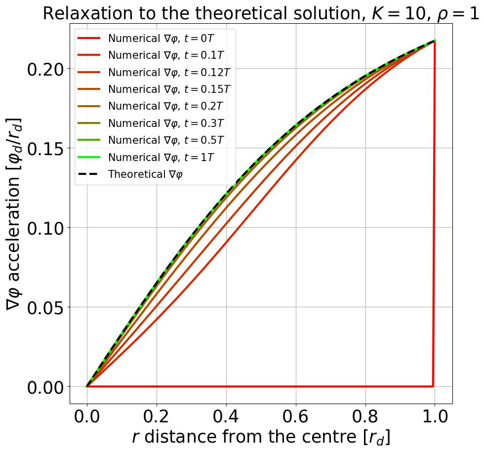
Figure 2. The numerical method shown to be relaxing to the stationary solution in the $\rho(r)=\rho_{0}$ solution, with $N=200$ and dimensionless values of $K=10$ and $\rho=1$.

To test the reliability of the numerical method, its results are compared to the theoretical results from eqs. 13, 24 and 23. Note that due to the nonlinear term, the numerical method and the theoretical solutions can only be compared with an opposite sign of $K$. The results are shown in Fig. 3.

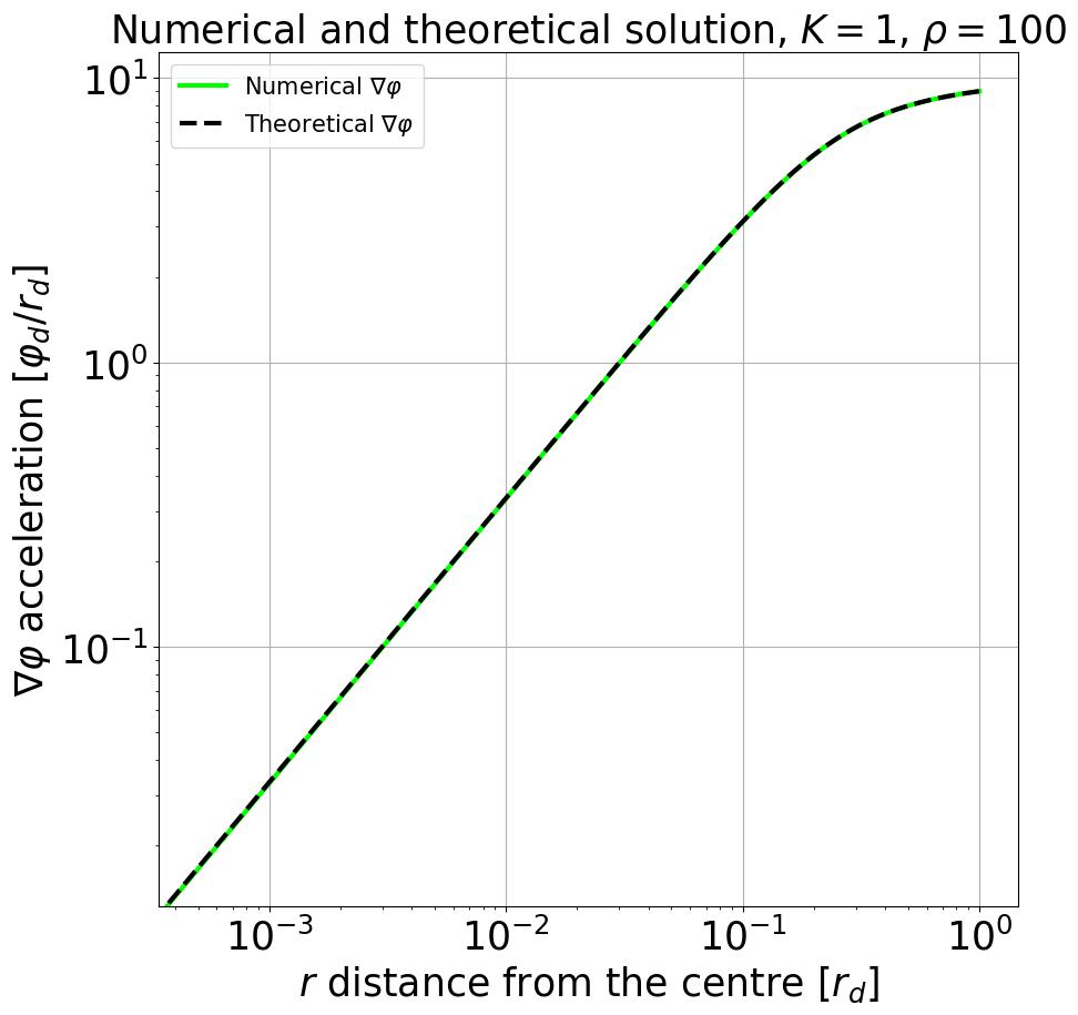
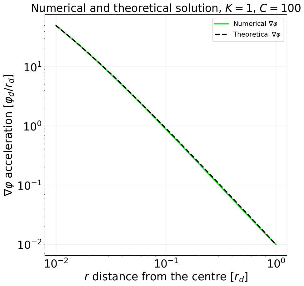
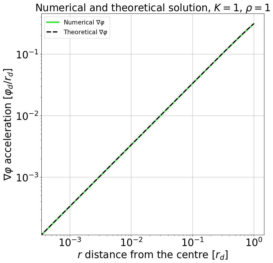
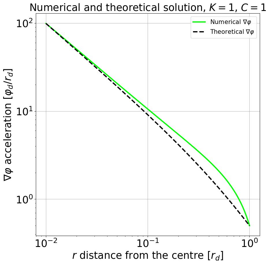
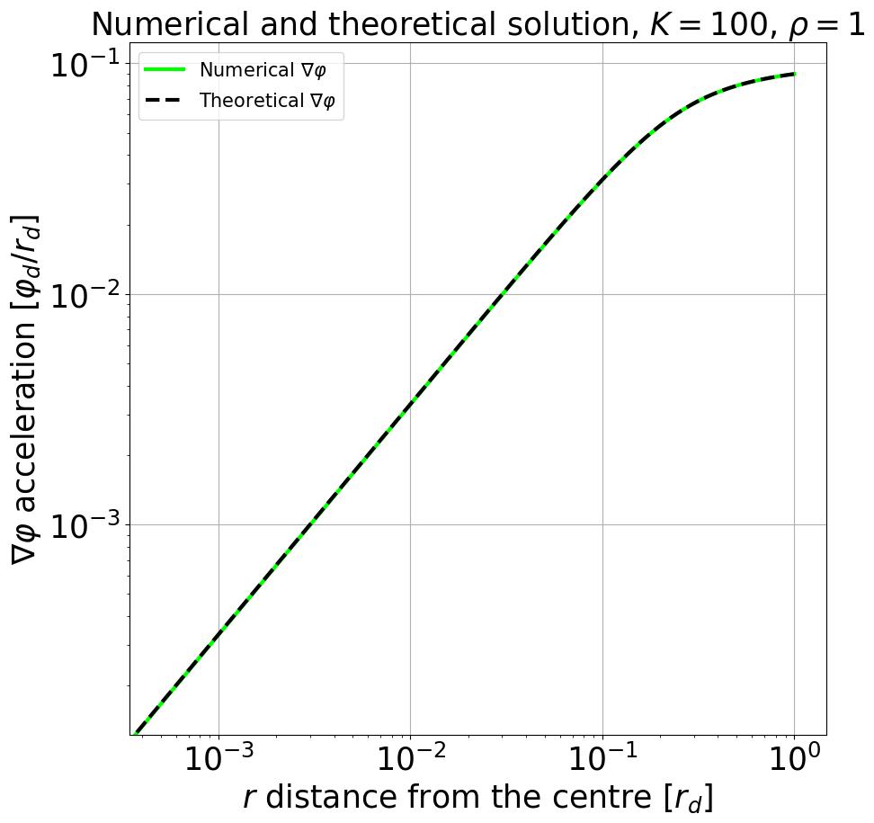
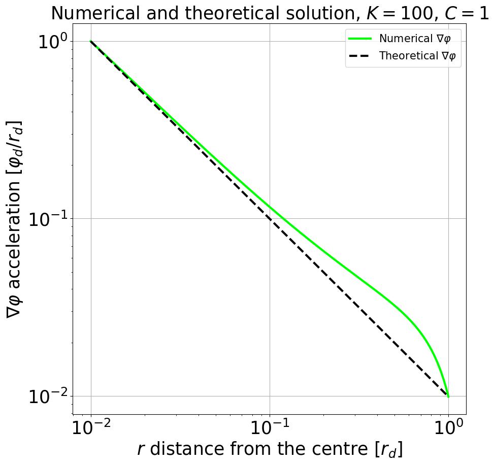
Figure 3. The result of the numerical method compared to the theoretical solution in the regimes of $K\ll\rho_{0}$, $K=\rho_{0}$ and $K\gg\rho_{0}$ for constant density and for $K\ll C$, $K=C$ and $K\gg C$ for vacuum.

We can see that the numerical solution reproduces the exact theoretical solution for constant density, but only reproduces the theoretical solution closer to the boundary for vacuum in the $K\ll C$ regime, that is, when the effect of the apparent mass is much greater than the effect of the nonlinear term. By choosing the appropriate scale, we can see the crossover as in [20] on Fig. 4.

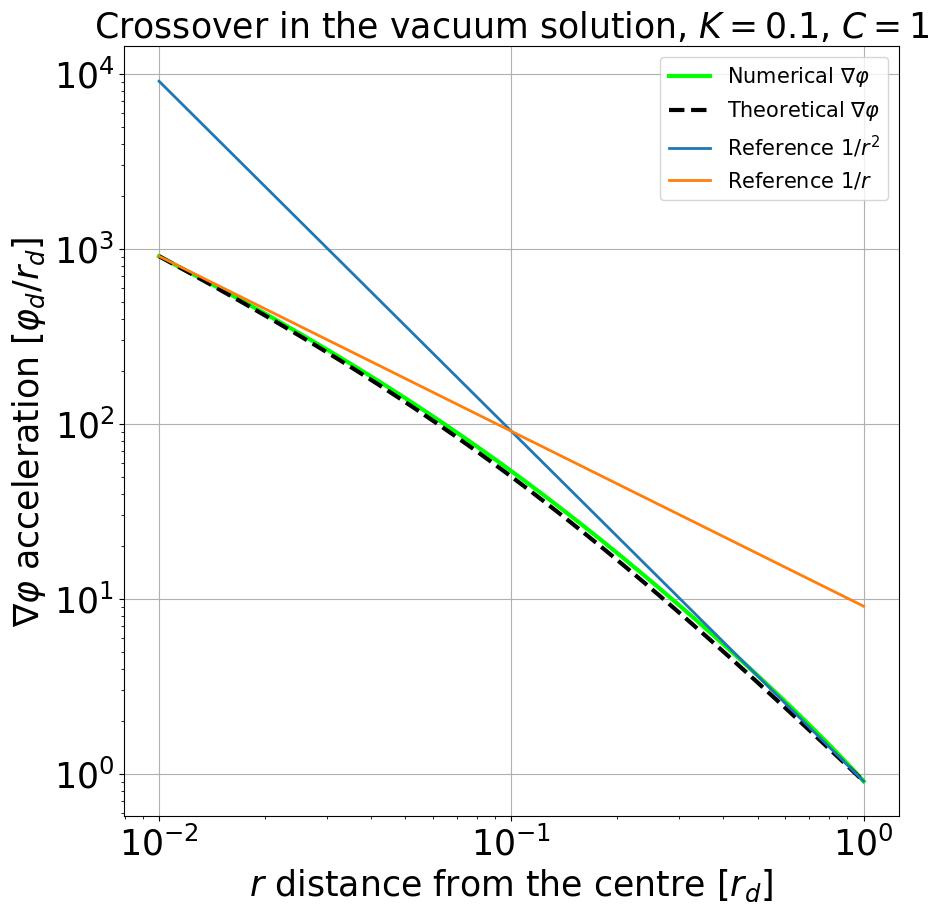
Figure 4. The crossover in the vacuum solution. Near the inner boundary, the $\frac{1}{Kr}$ term dominates, and at the outer boundary, the $\frac{1}{Cr^{2}}$ dominates. The resulting field looks Newtonian from far away, but with a greater mass, compared to the classical case.

Furthermore, the joint solution of a nonzero density core surrounded with vacuum is tested, where $\rho(r)=\rho_{c}$ in the interval $r\in[0,\frac{1}{2}r_{d})$, and $\rho(r)=0$ in the interval $r\in[\frac{1}{2}r_{d},r_{d}]$. To determine the $C$ parameter in the vacuum solution, the continuity of the derivative was prescribed:

(44) $$g_{\pm}\left(\frac{1}{2}r_{d}\right)=g_{vacuum}\left(\frac{1}{2}r_{d}\right),$$

(45) $$C=-\frac{4}{g_{\pm}\left(\frac{1}{2}r_{d}\right)r_{d}^{2}}-\frac{2K}{r_{d}}.$$

The boundary conditions are the corresponding constant density and vacuum derivatives. The numerical method is shown to reproduce the theoretical joint case in of dimensionless values $\rho_{c}=1$, $K=-10$ and $K=10$ in Fig. 5.

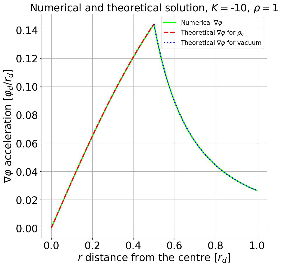
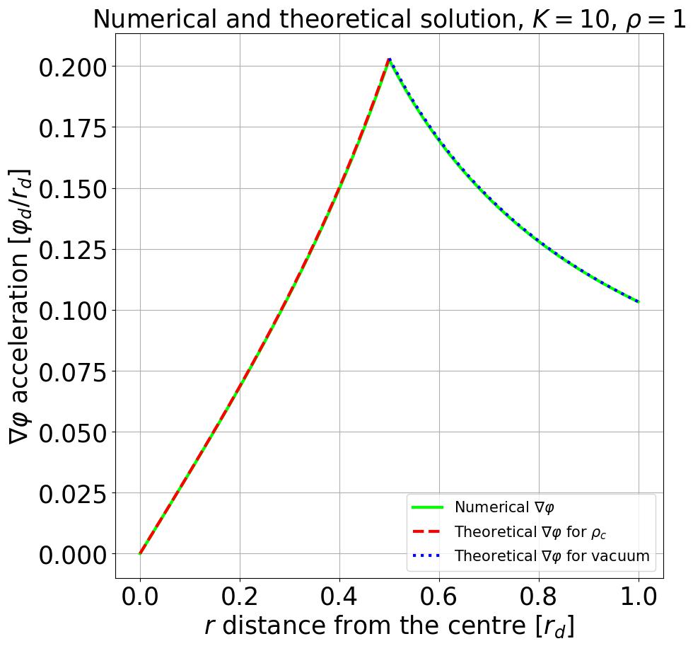
Figure 5. The result of the numerical method compared to the joint theoretical solutions in the case of dimensionless values $\rho_{c}=1$, $K=-10$ and $K=10$.

Therefore we can trust that the numerical solution for the thermodynamically modified gravitational field will be reliable for realistic mass distributions as well, as long as they have similar characteristic parameter relations. Larger $K$ values relative to $\rho_{c}$ result in negative $C$ as per eq. 45 and are unlikely to be physically meaningful as per eq. 16.

3. Analyses of rotational velocity curves

3.1. Methodology

To calculate velocity curves, the derivative field from the numerical solution is used to calculate the inferred rotational velocity, calculating the dimensional values:

(46) $$v_{j}=\left(\frac{\varphi_{d}}{r_{d}}\;r\;q_{j,T}\right)^{\frac{1}{2}}.$$

The velocities corresponding to the surface densities for atomic hydrogen (HI) and the stellar disk (SD) were converted into an equivalent pseudo-spherical dataset to calculate density data. The original velocities are defined as the velocities each component would induce in the plane of the galaxy, and for the comparison a spherical case is considered. The work by de Blok et al. [29] uses the convention that the negative sign of the HI data means that it has a negative contribution when calculating the total $v^{2}$ sum, that is, it has an outward gravitational effect due to the lack of spherical symmetry and the specifics of its distribution. The observed velocity curve data is based on the $21$-cm HI observations, the SD data is calculated from luminosity and the derived HI gas rotation curve is from the hydrogen column density. To calculate the $\rho_{j}$ for the numerical method from the interpolated function of the rotation velocities $v_{rot}(r)$, the following procedure was used:

(47) $$\rho_{j}=\left[\frac{\partial(v_{rot,SD}(r)^{2}r)}{\partial r}\right]_{j}\cdot\frac{1}{4\pi Gr_{j}^{2}}+\left[\frac{\partial(v_{rot,HI}(r)^{2}r)}{\partial r}\right]_{j}\cdot\frac{1}{4\pi Gr_{j}^{2}},$$

and $\rho_{d}$ was selected to be the mean of the array $\rho_{j}$:

(48) $$\rho_{d}=\mathrm{mean}(\rho_{j}),$$

(49) $$\tilde{\rho}_{j}=\frac{\rho_{j}}{\mathrm{mean}(\rho_{j})}.$$

For comparison, the pseudo-isothermal (ISO) DM halo model is used, as in the work of de Blok et al. [29] and Randriamampandry and Carignan [30]. This model has the density profile

(50) $$\rho_{\mathrm{ISO}}(r)=\rho_{0}\left[1+\left(\frac{r}{R_{C}}\right)^{2}\right]^{-1},$$

where $\rho_{0}$ is the central density and $R_{C}$ is the core radius of the halo. The corresponding dark matter rotation curve is given by

(51) $$v(r)=\sqrt{4\pi G\rho_{0}R_{C}^{2}\left[1-\frac{R_{C}}{r}\arctan\left(\frac{r}{R_{C}}\right)\right]}.$$

For the galactic calculation, the $\rho_{0}$ and $R_{C}$ parameters are taken from Table 3 of [29], which contains mass models with fixed mass-luminosity ratios ($Y^{3.6}_{*}$, denoting the $3.6$ $\mu$m band) and Diet-Salpeter stellar initial mass function. To obtain the velocity curve from the ISO DM model, the contributions of the SD and HI are added to this.

Regarding the MOND model, the method and data of Randriamampandry and Carignan are used, [30], which can be interpreted as the vacuum AQUAL solution substituted directly into the velocity calculation. The exact form of the interpolating function of MOND is not fixed by the theory itself and some forms work better in explaining certain phenomena. Zhao & Famaey [31] found that a simplified form of the interpolating function not only provides good fits to the observed rotational curves but also the derived mass/luminosity ratios are more compatible with those obtained from stellar populations synthesis models. In [30] this simple interpolating function of MOND is applied:

(52) $$\mu(x)=\frac{x}{1+x},$$

and the fitted velocity curve is given by

(53) $$v^{2}(r)=\sqrt{v_{SD}^{2}+v_{HI}^{2}}\cdot\sqrt{a_{0}\cdot r+v_{SD}^{2}+v_{HI}^{2}},$$

with $v_{SD}$ describing the contribution of the stellar disk (and bulge, if given separately) and $v_{HI}$ describing the contribution of the neutral hydrogen. The acceleration parameter, $a_{0}$, is fitted to the observational data using eq. 53.

3.2. Galactic rotational velocity curve of NGC 3198

In this section, the above-mentioned method is applied to reproduce the velocity curve of NGC 3198.

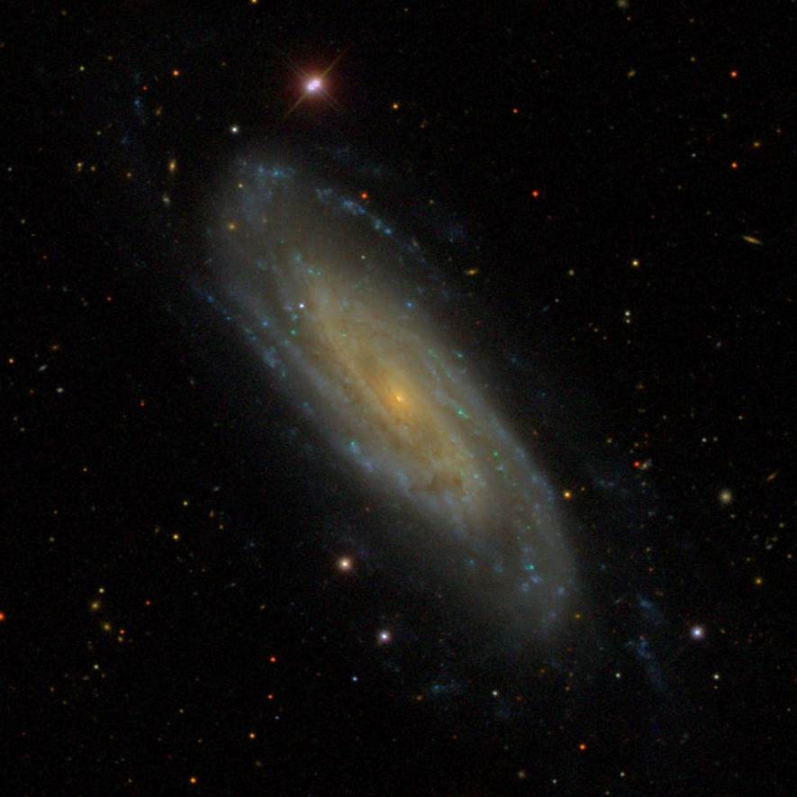
Figure 6. NGC 3198 galaxy, source: Sloan Digital Sky Survey.

NGC 3198
ISO Halo model
$\rho_{0}$ [$10^{-3}M_{\odot}pc^{-3}$]	$14.4\pm 2.0$
$R_{C}$ [$kpc$]	$4.97\pm 0.41$
MOND
$a_{0}$ [$10^{-10}ms^{-2}$]	$0.67\pm 0.02$
Thermodynamic gravity
$\tilde{K}$	$45$
$K$ [$s^{2}km^{-2}$]	$3.6\cdot 10^{-5}$

Figure 7. TG, MOND and ISO DM parameters for galaxy NGC 3198 [29].

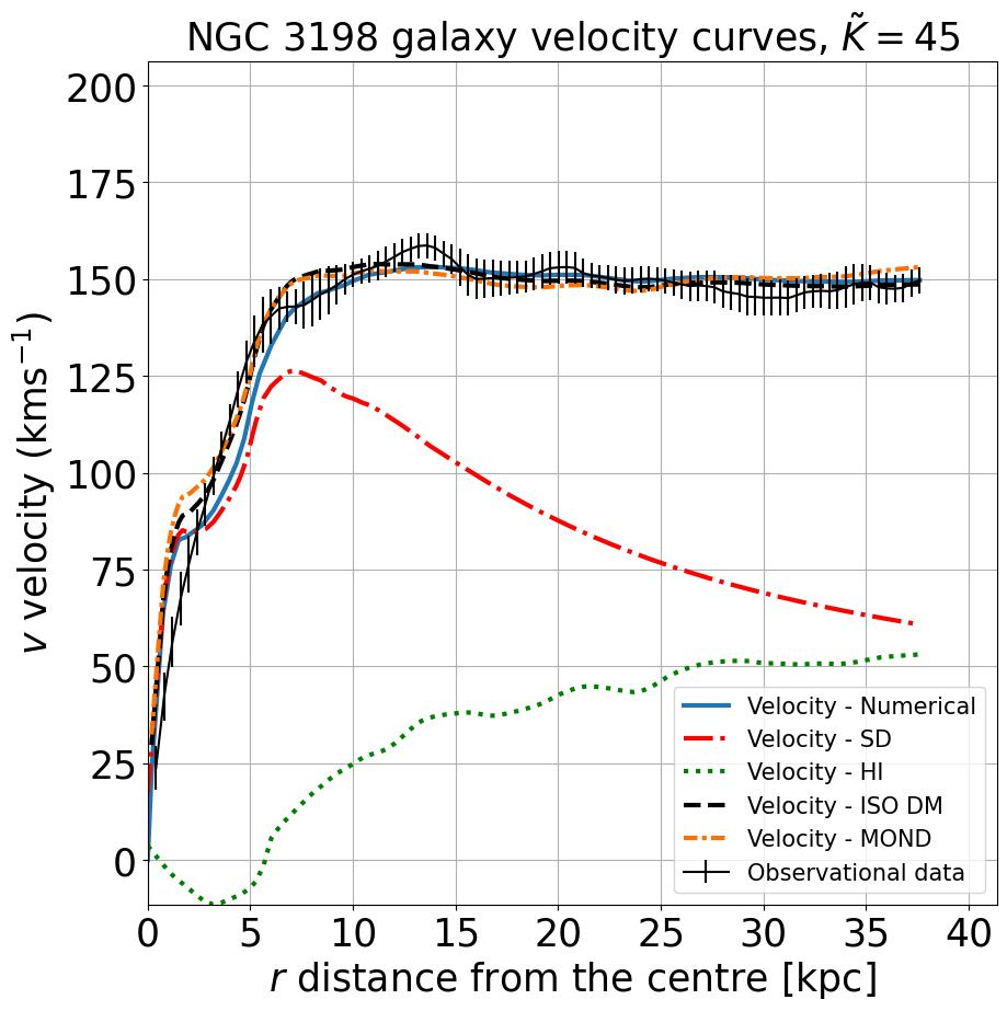
Figure 8. Velocity curves from thermodynamic gravity, MOND and ISO dark matter for the NGC 3198 galaxy.

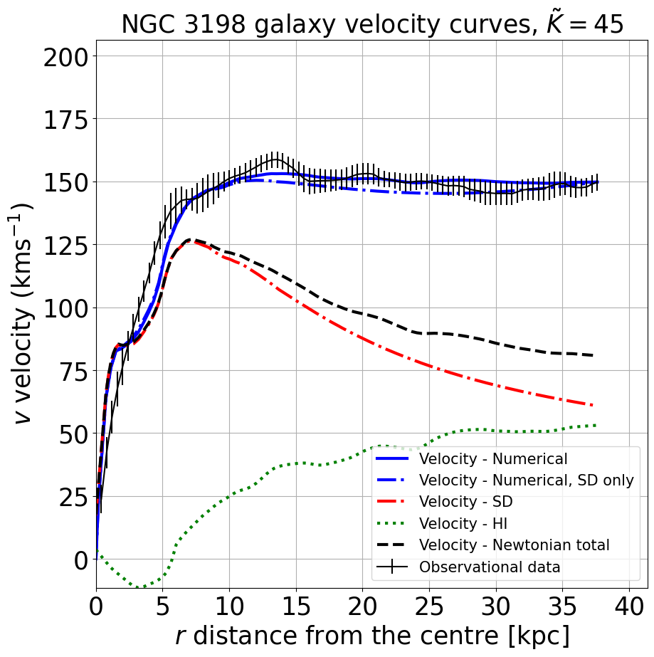
Figure 9. Velocity curves from thermodynamic gravity for galaxy NGC 3198 with the stellar disk mass distribution alone as the source for the gravitational field and the previous case with atomic H gas considered as well.

3.3. Discussion

NGC 3198 is a barred spiral galaxy known for its prototypical flat rotation curve, [32, 33, 34]. It was chosen because all three investigated theories provide a good fit for the observed velocity data. Additional galaxies will be investigated in future work. It is well-studied in the context of MOND, as the standard value of $a_{0}$ cannot predict the rotational velocity curve unless the distance of the galaxy is adjusted. Randriamampandry and Carignan found an acceptable MOND fit with $a_{0}$ about half the standard value. A much smaller distance is needed than the Cepheid-distance of $13.8$ Mpc [30]. As seen in Fig. 8, thermodynamic gravity can very similarly match the rotation curves of the ISO DM model and also of MOND, with $a_{0}$ being allowed to vary. A notable difference that TG seems to be more sensitive to the density distribution of the barionic matter, as it is apparent in the region where the density of the atomic hydrogen is negative, indicating the oversimplified nature of the spherical symmetric mass modell.

In TG, the $K$ parameter arising from the coupling can naturally vary between galaxies, allowing for a more versatile approach, while still having a strong foundation.

In Fig. 9 one can see separately the contribution of the neutral hydrogen to the velocity curve. One can see, that the contribution of atomic hydrogen is necessary for a proper modelling of the flat part.

3.4. Mass estimation

The datasets in the THINGS sample provide masses for the fitted mass models and using the fitted ISO DM parameters, the mass of the ISO DM halo can be calculated by integrating it up to the edge of the galaxy. For the purposes of this estimation, the edge of the galaxy will be considered to be at the last observational velocity curve datapoint ($r_{d}$). Using the insights from eqs. 13 and 16, by considering the fitted K parameters for the galaxy, it is possible to estimate the apparent asymptotic mass of the galaxy by setting the acceleration inferred from the edge of the galaxy to equal to the vacuum solution:

(54) $$\frac{v_{observed}(r_{d})^{2}}{r_{d}}=\frac{1}{Kr_{d}+Cr_{d}^{2}},$$

(55) $$C=\frac{1}{r_{d}}\left(\frac{1}{v_{observed}(r_{d})^{2}}-K\right),$$

(56) $$M_{aa}=\frac{v_{observed}(r_{d})^{2}}{1-Kv_{observed}(r_{d})^{2}}\frac{r_{d}}{G}.$$

In the case of $K=0$, eq. 56 should approximately yield the gravitating mass required for the observed velocity for the galaxy and is expected from the total mass inside $r_{d}$ with DM included. Therefore, we can call $M_{aa,K=0}$ as apparent total asymptotic mass of the galaxy. The values including dark matter or $M_{aa}$ are rounded to integers due to the large uncertainties included. Therefore, $M_{BM+ISO}$ inherits the uncertainty of $M_{ISO}$. The results are shown in Table 1:

Galaxy	$M_{SD}$	$M_{HI}$	$M_{total}$	$M_{ISO}$	$M_{BM+ISO}$	$M_{aa,K=0}$	$M_{aa}$
NGC 3198	$31.01$	$15.37$	$46.38$	$136\pm 19$	$183\pm 19$	$196$	$110$

Table 1. The mass components and estimates for ISO DM mass, all values are in the units of $10^{9}M_{\odot}$. $M_{SD}$ is the mass of the stellar components, $M_{HI}$ is the mass of neutral hydrogen, $M_{total}$ is the total mass of $M_{SD}$ and $M_{HI}$, $M_{ISO}$ is the mass of the ISO DM halo, integrated to $r_{d}$, $M_{BM+ISO}$ is the total mass, including baryonic and DM components, and $M_{aa}$ is the apparent asymptotic mass from the thermodynamic theory.

We can see, that the total baryonic and dark matter mass of NGC 3198, $M_{BM+ISO}$, is about the same as the apparent total mass of TG (expected at large distances), but the apparent asymptotic mass with the galactic $K$ value, $M_{aa}$, while differing from the ISO DM mass, up to $r_{d}$ results in the same gravitational effect. The characteristic $R$ spatial distance of the crossover, as pictured on Fig. 4 and detailed in [20] can be obtained as

(57) $$R=KGM_{aa},$$

according to eq. 17.

Using the $M_{aa,K=0}=196\cdot 10^{9}M_{\odot}$ mass for this scale, the expected characteristic crossover distance of this galaxy is $R\approx 60$ kpc, outside even of the extended data points of [35]. That is the distance where the flat velocity curve is expected to start declining and tending to a Newtonian one, which is determined by the vacuum solution of the Poisson equation with the apparent total asymptotic mass.

3.5. Conclusions

In this work, the analytical solutions of the nonlinear stationary field equation of TG were presented for the gravitational field in the cases of vacuum and constant matter density. Using the staggered grids-type discretisation, a numerical relaxation method was developed to solve the dissipative field equation of the theory. The stationary solution was obtained in the limit of the relaxation. The rotational velocity curve was calculated for galaxy NGC 3198 from the THINGS dataset, with only the baryonic matter contributing to the matter density source term [29].

It is remarkable, that NGC 3198 was previously investigated for the possible fits by MOND [30], and the ideally universal constant $a_{0}$ proved inadequate, as the best fits were only obtained when this parameter was allowed to vary, or the established distance of the galaxy was revised. The $K$ parameter in the theory investigated by this work arises from the coupling between the gravitational and mechanical thermodynamic forces and fluxes and, thus, naturally varies across the galaxies, depending on their smaller-scale dynamics and characteristics.

Based on the developed numerical method, a next step is to extend the analysis to other galaxies of the THINGS survey, with a detailed comparison of the alternative models. It is also natural to investigate thermodynamic gravity on the scale of galaxy clusters. It may be the case that on much larger scales, the theory has effects similar to Newtonian or general relativistic gravity, except the apparent mass is larger due to the thermodynamic coupling, with a crossover between the regimes [20].

The investigation of other challenging observed effects, such as gravitational lensing and the description of the fluid mechanics of the intracluster gas in the Bullet Cluster (1E 0657-56) are necessary to estimate the feasibility of a novel theory of gravity. In this respect, TG seems to be promising because the nonlinear field equation and the strong hydrodynamic coupling indicate that the lensing convergence can be non-zero where there is no projected matter, contrary to Einsteinian gravity, [36]. Also, the success of self-interacting dark matter investigations indicate the modelling potential of hydrodynamic approaches, [37]. Naturally, the Bullet Cluster, together with several other cosmological observations that have already been studied in the context of DM and MOND, require further research. The constitutive character of TG is an advantage when explaining and substituting the rich phenomenology of DM with modified gravity, [38].

For simplicity and analytical comparisons, the numerical method worked with a spherically symmetric model of mass distribution, although the baryonic mass of the non-elliptical galaxies usually has a more disk-shaped distribution, or more precisely, for HI a thin disk and for the stellar matter, a sech² distribution is chosen in de Blok [29]. In future work for more faithful results, the solutions in a cylindrical coordinate system with appropriate models can be considered, along with revisiting and possibly incorporating more precise considerations during the thermodynamic derivation of the dissipative field equation and more precise mass distribution models for the spherical DM halo, [39, 40].

Acknowledgements

We would like to thank Professor W. J. G. de Blok for providing us with the THINGS data [29]. We would also like to thank Professor S. Abe for providing insightful remarks regarding the theory.

The work was supported by the grants National Research, Development and Innovation Office – FK134277. The research reported in this paper is part of project no. BME-NVA-02, implemented with the support provided by the Ministry of Innovation and Technology of Hungary from the National Research, Development and Innovation Fund, financed under the TKP2021 funding scheme.

Data Availability

The data for the galaxy NGC 3198 used in this paper is based on the work of de Blok [29], DOI.: 10.1088/0004-6256/136/6/2648.

References

- [1] G. Bertone and T. M. P. Tait. A new era in the search for dark matter. Nature, 562(7725):51–56, oct 2018.
- [2] A. J. Krasznahorkay, M. Csatlós, L. Csige, J. Gulyás, A. Krasznahorkay, B. M. Nyakó, I. Rajta, J. Timár, I. Vajda, and N. J. Sas. New anomaly observed in supports the existence of the hypothetical X17 particle. Phys. Rev. C, 104:044003, Oct 2021.
- [3] A. Datta, R. Roshan, and A. Sil. Imprint of the Seesaw Mechanism on Feebly Interacting Dark Matter and the Baryon Asymmetry. Phys. Rev. Lett., 127:231801, Dec 2021.
- [4] B. Famaey and S. S. McGaugh. Modified Newtonian Dynamics (MOND): Observational Phenomenology and Relativistic Extensions. Living Reviews in Relativity, 15(1), 2012.
- [5] F. Lelli, S. S. McGaugh, J. M. Schombert, and M. S. Pawlowski. One Law to Rule Them All: The Radial Acceleration Relation of Galaxies. The Astrophysical Journal, 836(2):152, feb 2017.
- [6] P. Li, F. Lelli, S. McGaugh, and J. Schombert. Fitting the radial acceleration relation to individual SPARC galaxies. Astronomy & Astrophysics, 615:A3, 2018.
- [7] James S. Bullock and Michael Boylan-Kolchin. Small-Scale Challenges to the CDM Paradigm. Annual Review of Astronomy and Astrophysics, 55(1):343–387, 2017.
- [8] L. Berezhiani and J. Khoury. Theory of dark matter superfluidity. Physical Review D, 92(10):103510, 2015.
- [9] S. Hossenfelder. Covariant version of Verlinde’s emergent gravity. Phys. Rev. D, 95:124018, Jun 2017.
- [10] Horst Foidl, Tanja Rindler-Daller, and Werner W. Zeilinger. Halo formation and evolution in scalar field dark matter and cold dark matter: New insights from the fluid approach. Phys. Rev. D, 108:043012, Aug 2023.
- [11] K.G. Zloshchastiev. Galaxy rotation curves in superfluid vacuum theory. Pramana, 97(1):2, 2022.
- [12] T. C. Scott. From Modified Newtonian Dynamics to superfluid vacuum theory. Entropy, 25(1):12, 2022.
- [13] A. Maeder and V. G. Gueorguiev. The scale-invariant vacuum (SIV) theory: A possible origin of dark matter and dark energy. Universe, 6(3):46, 2020.
- [14] J. Bekenstein and M. Milgrom. Does the missing mass problem signal the breakdown of Newtonian gravity? The Astrophysical Journal, 286:7–14, November 1984.
- [15] P. Kroupa, B. Famaey, K. S. de Boer, J. Dabringhausen, M. S. Pawlowski, C. M. Boily, H. Jerjen, D. Forbes, G. Hensler, and M. Metz. Local-Group tests of dark-matter concordance cosmology - Towards a new paradigm for structure formation. A&A, 523:A32, 2010.
- [16] S. Dodelson. The real problem with MOND. International Journal of Modern Physics D, 20(14):2749–2753, 2011.
- [17] E. P. Verlinde. Emergent Gravity and the Dark Universe. SciPost Phys., 2:016, 2017.
- [18] S. Hossenfelder. Covariant version of verlinde’s emergent gravity. Physical Review D, 95(12):124018, 2017.
- [19] P. Ván and S. Abe. Emergence of extended Newtonian gravity from thermodynamics. Physica A: Statistical Mechanics and its Applications, 588:126505, 2022.
- [20] S. Abe and P. Ván. Crossover in Extended Newtonian Gravity Emerging from Thermodynamics. Symmetry, 14(5), 2022.
- [21] P. Ván. Holographic fluids: a thermodynamic road to quantum physics. Physics of Fluids, 35(5):057105, 2023. arXiv:2301.07177v2.
- [22] D. Giulini. Consistently implementing the field self-energy in Newtonian gravity. Physics Letters A, 232(3-4):165–170, 1997.
- [23] C. Sivaram, A. Kenath, and L. Rebecca. MOND, MONG, MORG as alternatives to dark matter and dark energy, and consequences for cosmic structures. Journal of Astrophysics and Astronomy, 41(1), February 2020.
- [24] L. Rebecca, A. Kenath, and C. Sivaram. Baryonic matter abundance in the framework of mong. Physical Sciences Forum, 7(1), 2023.
- [25] L. Diósi. Note on possible emergence time of Newtonian gravity. Physics Letters A, 377(31):1782 – 1783, 2013.
- [26] Kovács R. és Józsa V. Bevezetés a numerikus módszerekbe. Akadémiai Kiadó, 2019.
- [27] Á. Rieth, R. Kovács, and T. Fülöp. Implicit numerical schemes for generalized heat conduction equations. International Journal of Heat and Mass Transfer, 126:1177–1182, 2018.
- [28] Á. Pozsár, M. Szücs, R. Kovács, and T. Fülöp. Four spacetime dimensional simulation of rheological waves in solids and the merits of thermodynamics. Entropy, 22(12):1376, 2020.
- [29] W. J. G. de Blok, F. Walter, E. Brinks, C. Trachternach, S-H. Oh, and R. C. Kennicutt. High-Resolution Rotation Curves and Galaxy Mass Models from THINGS. The Astronomical Journal, 136(6):2648–2719, 2008.
- [30] T. H. Randriamampandry and C. Carignan. Galaxy mass models: MOND versus dark matter haloes. Monthly Notices of the Royal Astronomical Society, 439(2):2132–2145, 2014.
- [31] H. S. Zhao and B. Famaey. Refining the MOND Interpolating Function and TeVeS Lagrangian. The Astrophysical Journal, 638(1):L9, jan 2006.
- [32] T. S. van Albada, J. N. Bahcall, K. Begeman, and R. Sancisi. Distribution of dark matter in the spiral galaxy NGC 3198. The Astrophysical Journal, 295:305, August 1985.
- [33] E.V. Karukes, P. Salucci, and G. Gentile. The dark matter distribution in the spiral NGC 3198 out to 0.22 Rvir. Astronomy & Astrophysics, 578:A13, 2015.
- [34] G. Gentile, G.I.G. Józsa, P. Serra, G.H. Heald, W.J.G. de Blok, F. Fraternali, M.T. Patterson, R.A.M. Walterbos, and T. Oosterloo. HALOGAS: Extraplanar gas in NGC 3198. Astronomy & Astrophysics, 554:A125, 2013.
- [35] Gentile, G., Józsa, G. I. G., Serra, P., Heald, G. H., de Blok, W. J. G., Fraternali, F., Patterson, M. T., Walterbos, R. A. M., and Oosterloo, T. Halogas: Extraplanar gas in NGC 3198. Astronomy & Astrophysics, 554:A125, 2013.
- [36] G. W. Angus, B. Famaey, and HongSheng Zhao. Can MOND take a bullet? Analytical comparisons of three versions of MOND beyond spherical symmetry. Monthly Notices of the Royal Astronomical Society, 371(1):138–146, 2006.
- [37] Andrew Robertson, Richard Massey, and Vincent Eke. What does the Bullet Cluster tell us about self-interacting dark matter? Monthly Notices of the Royal Astronomical Society, 465(1):569–587, 10 2016.
- [38] P. Salucci. The distribution of dark matter in galaxies. The Astronomy and Astrophysics Review, 27(1), February 2019.
- [39] D. Giordano, P. Amodio, F. Iavernaro, A. Labianca, M. Lazzo, F. Mazzia, and L. Pisani. Fluid statics of a self-gravitating perfect-gas isothermal sphere. European Journal of Mechanics - B/Fluids, 78:62–87, 2019.
- [40] P.-H. Chavanis. The self-gravitating Fermi gas in Newtonian gravity and general relativity, 2021.