Convergence of SVRG-Extragradient for Variational Inequalities: Error Bounds and Increasing Iterate Averaging

Abstract

We study the last-iterate convergence of variance reduction methods for extragradient (EG) algorithms for a class of variational inequalities satisfying error-bound conditions. Previously, last-iterate linear convergence was only known under strong monotonicity. We show that EG algorithms with SVRG-style variance reduction, denoted SVRG-EG, attain last-iterate linear convergence under a general error-bound condition much weaker than strong monotonicity. This condition captures a broad class of non-strongly monotone problems, such as bilinear saddle-point problems commonly encountered in two-player zero-sum Nash equilibrium computation. Next, we establish linear last-iterate convergence of SVRG-EG with an improved guarantee under the weak sharpness assumption. Furthermore, motivated by the empirical efficiency of increasing iterate averaging techniques in solving saddle-point problems, we also establish new convergence results for SVRG-EG with such techniques.

1 INTRODUCTION

We study the variational inequality (VI) problem: find $z^{*}\in V$ such that

$$\langle F(z^{*}),z-z^{*}\rangle\geq 0,\;\forall\;z\in\mathcal{Z},$$ (VI)

where $V$ is some Euclidean space, $F:V\rightarrow V$ is a monotone operator, and $\mathcal{Z}$ is a compact convex set in $V$. A prominent use case of VIs is in addressing convex-concave saddle-point problems (SPPs):

$$\min_{x\in\mathcal{X}}\max_{y\in\mathcal{Y}}f(x,y),$$ (SP)

where $\mathcal{X}$ and $\mathcal{Y}$ are compact convex sets, and $f$ is a differentiable function with Lipschitz gradients. To transform (SP) into a VI, we let $z$ be the concatenation of $x$ and $y$, construct the monotone operator $F(z)=(\nabla f_{x}(x,y),-\nabla f_{y}(x,y))$, and $\mathcal{Z}=\mathcal{X}\times\mathcal{Y}$. Then, the set of optimal solutions $\mathcal{Z}^{*}$ corresponds to the set of saddle-points of (SP).

In this paper, we are particularly motivated by the SPPs that arise from two-player zero-sum games. In such games, the set of Nash equilibria is the set of solutions to an SPP, where ${\cal X},{\cal Y}$ represent the sets of possible mixed strategies for the respective players, and $f$ encodes the expected value attained by the second player given a strategy pair $(x,y)$. Notably, for both normal-form games (i.e. matrix games) and extensive-form games (EFGs), ${\cal X},{\cal Y}$ are compact convex polyhedral sets, and $f$ is a biaffine function. This configuration results in a VI characterized by an affine operator $F$ and a compact convex polyhedral set $\mathcal{Z}$.

In many real-world applications of VIs, the operator $F$ often exhibits a finite-sum structure, denoted as $F=F_{1}+\cdots+F_{N}$. Originally, the finite-sum structure was motivated by machine-learning problems, where it reflects the empirical risk across $N$ data points. Nonetheless, it can also arise from the decomposition of the payoff matrix in a normal-form game, or from the inherent structure of the payoff matrix based on expected values—as seen when cards are randomly dealt in the EFG representation of a poker game [27]. Stochastic first-order methods (FOMs) can leverage finite-sum structures to achieve convergence rates comparable to those of deterministic methods, while at a much lower cost per iteration. One such approach is known as stochastic variance reduced gradient (SVRG), which leverages the finite-sum structure when doing variance reduction.

We consider the SVRG extragradient method (SVRG-EG) for VIs, as proposed by Alacaoglu and Malitsky [1]. In particular, our focus is primarily on the loopless version of SVRG-EG. For this algorithm, Alacaoglu and Malitsky [1] showed that for a monotone VI, the uniform average of the iterates converges to a solution at a rate of $O(1/T)$, where $T$ is the number of iterations. Moreover, they showed that, when $\mathcal{Z}$ is a strongly convex set (or $F$ is strongly monotone, though they omitted the proof), the loopless SVRG-EG achieves last-iterate linear convergence.

We study convergence properties of SVRG-EG under more general assumptions. Firstly, we consider a classical error-bound condition (or simply error bounds). This condition generalizes the strong monotonicity assumption and captures a range of practical problems of interest where strong monotonicity does not hold, such as two-player zero-sum games and image segmentation [7]. We show that both the loopless SVRG-EG and its double-loop variant achieve linear convergence in their last iterates under the error-bound condition. To the best of our knowledge, our result is the first constant-stepsize stochastic FOM that solves two-player zero-sum games at a linear rate. Furthermore, we consider a class of VIs whose solution sets are subject to a weak sharpness condition. Under this condition, we show that SVRG-EG achieves a last-iterate linear convergence rate which parallels that achieved under the strong monotonicity of $F$.

In addition to evaluating last iterates, we study increasing iterate averaging schemes (IIAS) for SVRG-EG. Typically, most first-order methods for convex, but not strongly convex, problems are shown to have an ergodic convergence rate, meaning that the uniform average of the iterates attains some guarantee of convergence, whereas the individual iterates may not have such a guarantee. However, the uniform averaging of iterates is very conservative: in practice, the early iterates are of very poor quality, but there is rapid improvement in the iterates. By averaging uniformly, this improvement is only slowly integrated to the running average of iterates. It was shown by Gao et al. [15] that IIAS significantly bolsters the practical performance in various FOMs, including the mirror prox method [34], and the primal-dual method of Chambolle and Pock [7] and its variants [30, 8], while retaining the same theoretical guarantee of convergence. They pinpointed two particularly effective strategies: linear averaging, where the weight of iterate $t$ is proportional to $t$, and quadratic averaging, where the weight $t$ is proportional to $t^{2}$. We show that IIAS maintains the same $O(1/T)$ rate of convergence as that of the ergodic scheme presented by Alacaoglu and Malitsky [1] for SVRG-EG.

Finally, we study the numerical performance of SVRG-EG algorithms, under uniform averaging, linear averaging, and last iterate. We contrast that with state-of-the-art methods for solving SPPs, also instantiated with each of these averaging schemes. First, we demonstrate that the last iterates of SVRG-EG achieve fast convergence for both matrix games and EFGs. Second, we find that it is important to take into account IIAS: the deterministic and SVRG-EG methods have orders-of-magnitude performance differences depending on the averaging scheme. On matrix games we find that SVRG-EG methods with IIAS, or last-iterate, perform substantially better than other methods. On EFGs we find that SVRG-EG performs better than EG in one game and on par in another. For image segmentation, SVRG-EG with linear and last-iterate again perform substantially better than other methods.

2 RELATED WORK

For VIs and SPPs, EG-type methods are renowned for their strong convergence guarantees in the deterministic full-gradient setting. Convergence guarantees have been established for uniform iterate averaging (e.g., Nemirovski [34]) and the last iterate (e.g., Tseng [48]). There is also extensive literature on variations of EG that avoid taking two steps or avoid two gradient computations per iteration, and so on (e.g. Hsieh et al. [18], Malitsky and Tam [31]). That said, all of these full-gradient methods require one or more full gradient computations per iteration.

The rising significance of stochastic methods in large-scale computations has driven interest in stochastic EG methods. Juditsky et al. [22] studied stochastic Mirror-Prox (which generalizes EG) methods for VIs with compact convex feasible sets, and Mishchenko et al. [33] improved the algorithm by using a single sample per iteration. Hsieh et al. [18] showed stochastic variants of the single-call type EG methods. Yet, with a constant stepsize, the iterates of these methods only converge to a neighborhood of the solution set. Diminishing stepsizes do ensure convergence, but they empirically slow down the performance.

Variance reduction is a powerful mechanism to enhance the convergence rates of stochastic FOMs. A detailed discussion of SVRG and other variance reduction techniques in the context of convex minimization can be found in Appendix A. For solving saddle-point problems, SVRG-style variance reduction was first studied under the strongly-convex-concave setting by Palaniappan and Bach [39]. Since then, there has been extensive work on similar variance reduction techniques for the more general strongly monotone VIs [4, 2, 20]. However, these works do not easily extend to the setting we focus on, that is, non-strongly convex-concave—especially bilinear—saddle-point problems, a special form of non-strongly monotone VIs. It is worth noting, though, that one could apply Nesterov smoothing in order to reduce the monotone setting to the strongly monotone setting, at a small cost in theory [36]. An adaptive variant of that approach is given by Jin et al. [20]. However, here we are interested in methods such as EG, which avoid smoothing.

Carmon et al. [6] gave, to our knowledge, the first theoretical results for variance reduction in matrix games, a special case of monotone VIs. Huang et al. [19] considered monotone and strongly monotone VIs, and also developed SVRG-style methods. Han et al. [16] gave lower bounds for solving finite-sum saddle-point problems via FOMs. Note that their lower bounds do not contradict our linear-rate results: their analysis relies on non-polyhedral feasible sets such as $\ell_{2}$-norm balls. None of the works mentioned in this paragraph consider the error-bound condition for VIs and SPPs. Also, they do not incorporate non-uniform iterate averaging schemes.

Tseng [48] established a paradigm for deriving linear convergence for iterative methods in VIs, under the projection-type error-bound condition. Since then, error bounds have been commonly used in the analysis of FOMs. For more about this, see Drusvyatskiy and Lewis [12] and references therein. Recently, error bounds (or equivalent conditions) have also been considered to show linear convergence of SVRG methods without strong convexity, in the convex minimization setting, e.g., by Karimi et al. [24], Xu et al. [50], Zhang and Zhu [51].

Proposed by Polyak [41], the concept of a sharp solution was generalized by Burke and Ferris [5] to weak sharpness to include the possibility of multiple solutions. Patriksson [40] generalized weak sharpness to variational inequalities. While weak sharpness is often linked to identifying finite convergence [32], we aim to leverage this assumption to determine a specific rate at which iterates approach the solution set. In recent work, Applegate et al. [3] used sharpness to show linear convergence of first-order primal-dual methods for minimax problems. Note that, their assumption is not generally equivalent to ours, and they analyzed a different, and deterministic, algorithm.

3 PRELIMINARIES

Let $V$ be a finite dimensional vector space and $S$ be a nonempty closed convex set in $V$. Let $\langle\cdot,\cdot\rangle$ denote the Euclidean inner product and $\lVert\cdot\rVert$ denote the Euclidean norm. Denote the Euclidean projection of $z$ onto set $S$ as $\Pi_{S}(z)=\arg\min_{z^{\prime}\in S}\lVert z^{\prime}-z\rVert$. For a matrix ${\mathbf{A}}$, we denote its $i$’th row as ${\mathbf{A}}_{i}$ and $j$’th column as ${\mathbf{A}}_{\cdot j}$. ${\mathbf{A}}^{\top}$ is the transpose of ${\mathbf{A}}$. $\lVert{\mathbf{A}}\rVert_{F}$ is the Frobenius norm and $\lVert{\mathbf{A}}\rVert_{2}$ is the operator norm of ${\mathbf{A}}$ (induced by $\lVert\cdot\rVert_{2}$). $\mathbb{E}_{\xi}$ represents the expectation with respect to a random variable $\xi$. ${\cal F}=\sigma(\cdot)$ denotes $\sigma$-field generated by a set of random variables.

We assume (VI) satisfies the following assumptions:

Assumption 1.

The solution set $\mathcal{Z}^{*}$ is nonempty.

Assumption 2.

The subset $\mathcal{Z}\subset V$ is a compact convex set.

Assumption 3.

The operator $F$ is monotone, i.e., $\langle F(z_{1})-F(z_{2}),z_{1}-z_{2}\rangle\geq 0,\;\forall z_{1},z_{2}\in\mathcal{Z}$.

Assumption 4.

The operator $F$ has a stochastic oracle $F_{\xi}$ that is unbiased, i.e., $\mathbb{E}_{\xi}[F_{\xi}(z)]=F(z),\;\forall z\in\mathcal{Z}$ and $L_{f}$-Lipschitz in mean, i.e., $\mathbb{E}_{\xi}[\lVert F_{\xi}(z_{1})-F_{\xi}(z_{2})\rVert^{2}]\leq L^{2}\lVert z_{1}-z_{2}\rVert^{2},\;\forall z_{1},z_{2}\in\mathcal{Z}$.

While our results are somewhat more general, as in Alacaoglu and Malitsky [1], the primary application is the finite-sum setting where $F=F_{1}+\cdots+F_{N}$, in which case a natural stochastic oracle is one that samples an index $\xi\in[N]$, where $[N]=\{1,\ldots,N\}$. Throughout the paper, when we refer to $N$ it should be thought of as the number of terms in the finite-sum structure, or more generally the time to compute a full gradient relative to the computation of a gradient for a sample $\xi$.

4 ALGORITHM

This paper considers extragradient algorithms with variance reduction, first proposed by Alacaoglu and Malitsky [1]. We focus primarily on their loopless variant. Most results can be extended to their double-loop variant as well, but we defer the discussion on this to the appendix. The basic idea in (loopless) SVRG-EG is to maintain some intermittently-updated snapshot point $w_{k}$, which is updated stochastically with low probability. A full gradient is computed for $w_{k}$, and then the stochastic gradient estimates at each iteration use the gradient at the snapshot point combined with the gradient at the sampled index $\xi_{k}$ to perform variance reduction. This keeps the cost of most iterations cheap, while the variance of the gradient estimates reduces to $0$ as $k$ increases. This ensures that SVRG-EG converges with a constant stepsize. Beyond that, we can set adaptive (greater than $\tau_{0}$) stepsizes to exploit the feature of reduced variance to improve the convergence rate.

Input: $p\in(0,1]$, probability distribution ${\cal D}$, step size $\tau$, $\alpha\in(0,1)$, $z_{0}=w_{0}$

for $k=0,1,\cdots$ do

       $\bar{z}_{k}=\alpha z_{k}+(1-\alpha)w_{k}$;

       $z_{k+1/2}=\Pi_{\mathcal{Z}}(\bar{z}_{k}-\tau F(w_{k}))$;

       Draw an index $\xi_{k}$ according to ${\cal D}$;

       $\hat{F}(z_{k+1/2})=F_{\xi_{k}}(z_{k+1/2})-F_{\xi_{k}}(w_{k})+F(w_{k})$;

       $z_{k+1}=\Pi_{\mathcal{Z}}(\bar{z}_{k}-\tau\hat{F}(z_{k+1/2}))$;

       $w_{k+1}=\begin{cases}z_{k+1}&\text{with probability }p\\ w_{k}&\text{otherwise}.\end{cases}$

end for

Algorithm 1 SVRG-Extragradient (SVRG-EG)

We state the loopless SVRG-EG algorithm [1, Algorithm 1] in Algorithm 1. We have several important parameters: the probability $p$ to update $w_{k}$ at each iteration, the probability distribution $Q$ on the indices $\xi$ which defines the stochastic oracle, a step size $\tau_{0}$, and the convex combination parameter $\alpha$ which specifies the extent to which the centering point $\bar{z}_{k}$ moves towards the snapshot point $w_{k}$. In practice, we run these algorithms with the suggested parameters from Alacaoglu and Malitsky [1]. That is, we use $p=\frac{2}{N}$, $\alpha=1-\frac{2}{N}$ and $\tau=\frac{0.99\sqrt{2}}{\sqrt{N}L}$.

5 LINEAR CONVERGENCE UNDER ERROR BOUNDS

There is a variety of possible error-bound conditions in the literature. At a high level, they usually state that the distance to the solution set from a feasible point near the solution set can be bounded by some simple function of the feasible point, often the norm of an “iterative residual” term at that point. They are useful in establishing linear convergence guarantees for first-order methods, since they capture the distance to optimality using a distance-like measure for consecutive iterates.

We define the proximal-gradient mapping $\mathcal{G}_{\tau}(z)=\tau^{-1}\left(z-\Pi_{\mathcal{Z}}\left(z-\tau F(z)\right)\right)$. Using $\mathcal{G}_{\tau}(z)$ as the residual function, we assume a projection-type error-bound condition [48, Equation (5)]:

Assumption 5 (Error-Bound Condition).

The operator $F$ satisfies: given some $\tau\in(0,+\infty)$, we have

$$\textnormal{dist}(z,\mathcal{Z}^{*})\leq C_{0}\lVert\mathcal{G}_{\tau}(z)\rVert,\ \forall\;z\in\mathcal{Z}\text{ s.t. }\lVert\mathcal{G}_{\tau}(z)\rVert\leq\epsilon_{0},$$

for some $C_{0},\epsilon_{0}>0$, where we let $\textnormal{dist}(z,\mathcal{Z}^{*})=\min_{z^{*}\in\mathcal{Z}^{*}}\lVert z-z^{*}\rVert.$

Note that, $C_{0},\epsilon_{0}$ are $\tau$-invariant in this assumption.

In convex optimization and VI literature, the error-bound condition is often stated as a local property within a neighborhood around the optimal set. However, for problems with a bounded feasible set, we can easily extend it to the entire feasible set, as stated in the following lemma.

Lemma 1.

If Assumption Error-Bound Condition holds, then for any $z\in\mathcal{Z}$ and $\tau>0$, we have

$$\lVert z-\Pi_{\mathcal{Z}^{*}}(z)\rVert\leq C\lVert z-\Pi_{\mathcal{Z}}(z-\tau F(z))\rVert,$$ (1)

where $\bar{C}=\max\left\{C_{0},{D(\mathcal{Z})}/{\epsilon_{0}}\right\}$ and $C={\bar{C}}/{\tau}$. Here, $D(\mathcal{Z})$ is the maximal diameter of the compact set $\mathcal{Z}$.

Note that for each $z$, (1) only holds for the solution $\Pi_{\mathcal{Z}^{*}}(z)$ (closest to $z$) and, in general, different $z$ yield different solutions $\Pi_{\mathcal{Z}^{*}}(z)$. This is one of the most challenging issues in extending the proof of linear convergence under strong monotonicity from Alacaoglu and Malitsky [1] to the more relaxed error-bound condition (1), because the strong monotonicity holds for any pair of feasible points.

For our convergence analysis, we define a Lyapunov function combining both iterate point $z_{k}$ and snapshot point $w_{k}$ with a weight parameter $\theta\in[0,1]$: $\Phi^{\theta}_{z}(z_{k},w_{k})=\theta\lVert z_{k}-z\rVert^{2}+(1-\theta)\lVert w_{k}-z\rVert^{2}$ for any $z\in\mathcal{Z}$ and a corresponding projection onto the solution set $\Pi^{\theta}_{\mathcal{Z}^{*}}(z_{k},w_{k})=\mathrm{argmin}_{z^{*}\in\mathcal{Z}^{*}}\Phi^{\theta}_{z^{*}}(z_{k},w_{k})$. We define the distance from the iterate $(z_{k},w_{k})$ to the solution set $\mathcal{Z}^{*}$ as

$$\text{dist}^{\theta}_{\mathcal{Z}^{*}}(z_{k},w_{k})=\min\nolimits_{z^{*}\in\mathcal{Z}^{*}}\Phi^{\theta}_{z^{*}}(z_{k},w_{k}).$$ (2)

Using the above notation and a sequence of auxiliary iterates $\tilde{z}_{k+1/2}=\Pi_{\mathcal{Z}}(\bar{z}_{k}-\tau F(\bar{z}_{k}))$, we can derive another error-bound condition under the weighted distance (2), formalized in the following lemma.

Lemma 2.

Assume Assumptions 1-4 and Error-Bound Condition hold. Let $\alpha\in[0,1),\tau=\gamma\frac{\sqrt{1-\alpha}}{L}$, for $\gamma\in(0,1)$, and $\theta\in[0,1]$. Then, for each $k\geq 1$, Algorithm 1 ensures

$$\tau^{2}\frac{\alpha L^{2}}{6\bar{C}^{2}\alpha L^{2}+8}\textnormal{dist}^{\theta}_{\mathcal{Z}^{*}}(z_{k},w_{k})\leq\alpha\lVert z_{k}-z_{k+1/2}\rVert^{2}+(1-\alpha)\lVert w_{k}-z_{k+1/2}\rVert^{2},$$ (3)

where $\bar{C}$ is defined in Lemma 1.

Lemma 2 paves the way for our main linear convergence theorem. We state the result here and give a proof sketch; the full proof is in Section B.2. See similar results for the double-loop version of SVRG-EG in Section B.3.

Theorem 1.

Assume Assumptions 1-4 and Error-Bound Condition hold. Let $\{z_{k},w_{k}\}_{k\in\mathbb{N}_{+}}$ be iterates generated by Algorithm 1 with $p\in(0,1]$, $\alpha\in[0,1),\tau=\gamma\frac{\sqrt{1-\alpha}}{L}$, for $\gamma\in(0,1)$. Then, let $\theta=\frac{\alpha}{\alpha+\frac{1-\alpha}{p}}$, we have

$$\mathbb{E}\left[\textnormal{dist}^{\theta}_{\mathcal{Z}^{*}}(z_{k+1},w_{k+1})\right]\leq\rho\mathbb{E}\left[\textnormal{dist}^{\theta}_{\mathcal{Z}^{*}}(z_{k},w_{k})\right],$$ (4)

where $\rho=1-\tau^{2}\frac{(1-\gamma)\alpha L^{2}}{(4\bar{C}^{2}\alpha L^{2}+8)(\alpha+\frac{1-\alpha}{p})}$.

Proof sketch of Theorem 1.

We start from a crucial iteration decrease inequality in Alacaoglu and Malitsky [1, Eq. 10] without dropping $\lVert z_{k}-z_{k+1/2}\rVert^{2}$ term:

$$\mathbb{E}_{k}{\lVert z_{k+1}-z^{*}\rVert}^{2}\leq \alpha{\lVert z_{k}-z^{*}\rVert}^{2}+(1-\alpha){\lVert w_{k}-z^{*}\rVert}^{2}-(1-\alpha)(1-\gamma){\lVert z_{k+1/2}-w_{k}\rVert}^{2}$$

$$\hskip 80.0pt-(1-\gamma)\mathbb{E}_{k}{\lVert z_{k+1}-z_{k+1/2}\rVert}^{2}-\alpha{\lVert z_{k+1/2}-z_{k}\rVert}^{2}$$

for any $z^{*}\in\mathcal{Z}^{*}$. In the proof, $\mathbb{E}_{k}[\cdot]$ and $\mathbb{E}_{k+1/2}[\cdot]$ are the expectations w.r.t. $\mathcal{F}_{k}=\sigma(z_{0},w_{0},\ldots,z_{k},w_{k})$ and $\mathcal{F}_{k+1/2}=\sigma(z_{0},w_{0},\ldots,z_{k},w_{k},z_{k+1})$, respectively. $\mathbb{E}[\cdot]$ is the total expectation w.r.t. $\mathcal{F}_{0}$.

After applying Lemma 2 with a specific weight $\theta={\alpha}/({\alpha+\frac{1-\alpha}{p}})$ at each iteration we partially offset the terms (on the left-hand side) measuring the distance from the current iterates to the solution set.

By using $\mathbb{E}_{k+1/2}\lVert w_{k+1}-z\rVert^{2}=p\lVert z_{k+1}-z\rVert^{2}+(1-p)\lVert w_{k}-z\rVert^{2}$ for any $z\in\mathcal{Z}$ to handle the random update of snapshots, we transform the distance measure to the form of the Lyapunov function. After taking total expectation and applying the tower property, it yields that

$$\mathbb{E}\Big{[}\alpha\lVert z_{k+1}-z^{*}_{k}\rVert^{2}+\frac{1-\alpha}{p}\lVert w_{k+1}-z^{*}_{k}\rVert^{2}\Big{]}\leq\rho\mathbb{E}\Big{[}\alpha\lVert z_{k}-z^{*}_{k}\rVert^{2}+\frac{1-\alpha}{p}\lVert w_{k}-z^{*}_{k}\rVert^{2}\Big{]}.$$

Finally, we set $z^{*}_{k}=\Pi^{\theta}_{\mathcal{Z}^{*}}(z_{k},w_{k})$ and leverage the definition of projection based on our Lyapunov function to obtain that Equation 4.

Remark.

It is vital to determine the right $z^{*}_{k}$ and $\theta$ because our VI setting allows multiple solutions. Note that the error-bound assumption only applies to the specific solution minimizing the distance to some feasible point. Unlike Alacaoglu and Malitsky [1], we cannot use one fixed solution when we sum over a sequence of indices. Instead, we need to pick $z^{*}_{k}=\Pi_{\mathcal{Z}^{*}}^{\theta}(z_{k},w_{k})$.

Based on the nature of randomized methods, we say a randomized algorithm reaches $\epsilon$-accuracy if the expected distance to the solution set is under $\epsilon$. We show the time complexity results of the algorithms following this convention.

Corollary 1.

Set $p=\frac{2}{N}$, $\alpha=1-\frac{2}{N}$ and $\tau=\frac{0.99\sqrt{2}}{\sqrt{N}L}$ in Algorithm 1. Then, the time complexity to reach $\epsilon$-accuracy is $\mathcal{O}\left((N+\bar{C}^{2}NL^{2})\mathop{{\rm log}}{\frac{1}{\epsilon}}\right)$.

Though, with the fixed stepsize, we reach the same time complexity as the deterministic extragradient method (which needs a $O(N)$ time complexity because of its full gradient computing per iteration), SVRG-EG converges much faster numerically.

Note that the convergence rate per iteration is affected by the small fixed stepsizes we used in analysis, while in practice we can usually use a much larger stepsize.

6 LINEAR CONVERGENCE UNDER WEAK SHARPNESS

In this section, we consider the weak sharpness condition for (solution sets of) VIs and show that it is sufficient for the linear convergence of SVRG-EG. As discussed in Section 2, this condition extends the classical geometric definition for convex minimization problems. To state these conditions, we need additional notation. Denote $\mathcal{Z}^{\circ}:=\left\{v\in V:\langle v,z\rangle\leq 0\quad\forall\;z\in\mathcal{Z}\right\}$ as the polar set of $\mathcal{Z}\subseteq V$. If $\mathcal{Z}$ is a convex set and $z\in\mathcal{Z}$, the normal cone of $\mathcal{Z}$ at $z$ is $N_{\mathcal{Z}}(z):=\left\{v\in V:\langle v,w-z\rangle\leq 0\quad\forall\;w\in\mathcal{Z}\right\}$ and the tangent cone of $\mathcal{Z}$ at $z$ is $T_{\mathcal{Z}}(z):=[N_{{\mathcal{Z}}(z)}]^{\circ}$. Denote $\textnormal{int}(\mathcal{Z})$ as the interior of the set $\mathcal{Z}$. Let $\mathcal{Z}^{*}$ be the solution set of VI, the weak sharpness condition of $\mathcal{Z}^{*}$ is defined as follows [40]:

Assumption 6 (Weak Sharpness).

The operator $F$ satisfies:

$$-F(z^{*})\in\textnormal{int}\left(\bigcap_{z^{\prime}\in\mathcal{Z}^{*}}\big{[}\,T_{\mathcal{Z}}(z^{\prime})\cap N_{\mathcal{Z}^{*}}(z^{\prime})\,\big{]}^{\circ}\right),$$ (5)

for all $z^{*}\in\mathcal{Z}^{*}$.

Here, we give a simple example satisfying weak sharpness.

Example.

Consider $x=(x_{1},x_{2})\in\mathbb{R}^{2}$ and a monotone operator $F(x)=(\frac{x_{1}+x_{2}}{2}-2,\,\frac{x_{1}+x_{2}}{2}-2)$ and $\mathcal{X}=\{x\,|\,0\leq x\leq 1,x_{1}+x_{2}\leq\frac{3}{2}\}$. One can verify that the corresponding VI has a solution set $\mathcal{X}^{*}=\{x\,|\,\frac{1}{2}\leq x_{1}\leq 1,x_{1}+x_{2}=\frac{3}{2}\}$. For $x^{*}\in\mathcal{X}^{*}\setminus\{(\frac{1}{2},1),(1,\frac{1}{2})\}$, $T_{\mathcal{X}}(x^{*})=\{x\,|\,x_{1}+x_{2}\leq 0\}$ and $N_{\mathcal{X}^{*}}(x^{*})=\{x\,|\,x_{1}=x_{2}\}$, thus $[T_{\mathcal{X}}(x^{*})\cap N_{\mathcal{X}^{*}}(x^{*})]^{\circ}=\{x\,|\,x_{1}+x_{2}\geq 0\}$. For $x^{*}=(\frac{1}{2},1)$, $T_{\mathcal{X}}(x^{*})=\{x\,|\,x_{2}\leq 0,x_{1}+x_{2}\leq 0\}$ and $N_{\mathcal{X}^{*}}(x^{*})=\{x\,|\,x_{2}-x_{1}\geq 0\}$, thus $[T_{\mathcal{X}}(x^{*})\cap N_{\mathcal{X}^{*}}(x^{*})]^{\circ}=\{x\,|\,x_{2}\geq 0,x_{1}+x_{2}\geq 0\}$. Similarly, for $x^{*}=(1,\frac{1}{2})$, $[T_{\mathcal{X}}(x^{*})\cap N_{\mathcal{X}^{*}}(x^{*})]^{\circ}=\{x\,|\,x_{1}\geq 0,x_{1}+x_{2}\geq 0\}$. Hence, $\bigcap_{x^{*}\in\mathcal{X}^{*}}[T_{\mathcal{X}}(x^{*})\cap N_{\mathcal{X}^{*}}(x^{*})]^{\circ}=\mathbb{R}^{2}_{+}$. Obviously, $-F(x^{*})=-(\frac{5}{4},\frac{5}{4})\in\textnormal{int}(\bigcap_{x^{*}\in\mathcal{X}^{*}}[T_{\mathcal{X}}(x^{*})\cap N_{\mathcal{X}^{*}}(x^{*})]^{\circ})$. Therefore, the corresponding VI satisfies weak sharpness. Note that this VI does not satisfy strong monotonicity since $\langle F(x)-F(y),x-y\rangle=(x_{1}-y_{1}+x_{2}-y_{2})^{2}/2$.

Under this assumption, we have the following property, which is essential in our proof.

Lemma 3.

If the solution set of the VI satisfies Weak Sharpness, then there exists a $\mu$ such that

$$\langle F(z^{*}),\,z-\Pi_{\mathcal{Z}^{*}}(z)\rangle\geq\mu\lVert z-\Pi_{\mathcal{Z}^{*}}(z)\rVert,$$ (6)

for any $z\in\mathcal{Z},z^{*}\in\mathcal{Z}^{*}$.

Note that this can be interpreted as an error-bound condition which says that the distance between $z$ and $\mathcal{Z}^{*}$ is bounded by some residual term. We then leverage this property of weak sharpness to derive the linear convergence rate and the resulting logarithmic time complexity of SVRG-EG. See the proof in Appendix C.

Theorem 2.

Let Assumptions 1-4 and Weak Sharpness hold. Let $\{z_{k},w_{k}\}_{k\in\mathbb{N}_{+}}$ be iterates generated by Algorithm 1 with $p\in(0,1]$, $\alpha\in[\frac{1}{2},1),\tau=\gamma\frac{\sqrt{1-\alpha}}{L}$, for $\gamma\in(0,1)$. Then, let $\theta=\frac{\alpha}{\alpha+\frac{1-\alpha}{p}}$, we have

$$\mathbb{E}_{k}\left[\textnormal{dist}^{\theta}_{\mathcal{Z}^{*}}(z_{k+1},w_{k+1})\right]\leq\rho^{\textnormal{WS}}\textnormal{dist}^{\theta}_{\mathcal{Z}^{*}}(z_{k},w_{k}),$$ (7)

where $\rho^{\textnormal{WS}}=1-\frac{c}{2(\alpha+\frac{1-\alpha}{p})}$ and $c=\min\{\tau\frac{\mu}{D(\mathcal{Z})},\,(1-\gamma)(1-\alpha)\}$.

Corollary 2.

Set $p=\frac{2}{N}$, $\alpha=1-\frac{2}{N}$ and $\tau=\frac{0.99\sqrt{2}}{\sqrt{N}L}$ in Algorithm 1. Then, the time complexity to reach $\epsilon$-accuracy is $\mathcal{O}\left((N+\frac{\sqrt{N}L}{\mu})\mathop{{\rm log}}{\frac{1}{\epsilon}}\right)$.

Remark.

Though weak sharpness results in a better dependence on $N$ in the convergence rate compared to that of the deterministic EG method in Tseng [48], it is more restrictive than the error-bound condition. In particular, it does not hold for bilinear saddle-point problems in general.

7 INCREASING ITERATE AVERAGING SCHEMES

The main convergence guarantees given in Alacaoglu and Malitsky [1] are for the uniform averages of iterates. However, empirically the uniform average of iterates rarely performs well. In contrast, as shown in Gao et al. [15], when solving saddle-point problems using first-order algorithms such as the deterministic EG method, increasingly-weighted averages often outperform uniform averages numerically while having the same theoretical convergence guarantees.

Motivated by such empirical evidence, we show that Algorithm 1 preserves the $O(1/T)$ rate of convergence when using increasing iterate averaging. In particular, we establish a $O(1/T)$ convergence rate for SVRG-EG with polynomial (e.g. uniform, linear, quadratic or cubic) weighted iterate averaging. We also provide the same results for double-loop SVRG-EG, which can be found in Appendix D.3.

Here, we consider the generalized variational inequality problem: to find $z^{*}\in V$ such that

$$\langle F(z^{*}),z-z^{*}\rangle+g(z)-g(z^{*})\geq 0,\;\forall\;z\in V,$$ (GVI)

which is subject to the following assumptions:

Assumption 7.

The solution set of GVI is nonempty.

Assumption 8.

The function $g$ is a proper convex lower semicontinuous function.

Assumption 9.

The operator $F$ is monotone, i.e., $\langle F(z_{1})-F(z_{2}),z_{1}-z_{2}\rangle\geq 0,\;\forall z_{1},z_{2}\in\textnormal{dom}\,g$.

Assumption 10.

The operator $F$ has a stochastic oracle $F_{\xi}$ that is unbiased, i.e., $\mathbb{E}_{\xi}[F_{\xi}(z)]=F(z),\;\forall z\in V$ and $L$-Lipschitz in mean, i.e., $\mathbb{E}_{\xi}[\lVert F_{\xi}(z_{1})-F_{\xi}(z_{2})\rVert^{2}]\leq L^{2}\lVert z_{1}-z_{2}\rVert^{2},\;\forall z_{1},z_{2}\in V$.

The classical VI can be reduced from GVI by letting $g=0$ if $z\in\mathcal{Z}$ and $+\infty$ otherwise. Correspondingly, using

$$\textnormal{Prox}_{\tau g}(z)=\arg\min_{z^{\prime}\in V}\left\{\frac{1}{2}\lVert z^{\prime}-z\rVert^{2}+\tau g(z^{\prime})\right\}$$

to replace $\Pi_{\mathcal{Z}}(z)$ in Algorithm 1, we can adapt SVRG-EG to solve GVI. As is typical in the analysis of the convergence of algorithms for VIs, we chose the following gap function as the convergence measure: $\textnormal{Gap}(w)=\max_{z\in{\cal C}}\left\{\left\langle F(z),w-z\right\rangle+g(w)-g(z)\right\}$. Here, ${\cal C}\subseteq V$ is a compact subset, which allows possible unboundedness of $\text{dom}\,g$ (see Nesterov [37, Lemma 1]). The gap function is well-defined, convex, and equal to $0$ when $w$ is a solution to (VI).

To analyze the convergence of SVRG-EG under increasing iterate averaging, we need to extend Alacaoglu and Malitsky [1, Lemmas 2.2 & 2.4] to handle non-uniform iterate weights.

Lemma 4.

Assume Assumptions 7-10 hold. Let $z_{k},w_{k},z_{k+1/2}$ be iterates generated by loopless SVRG-EG with $p\in(0,1]$, $\alpha\in[0,1)$, $\tau=\frac{\sqrt{1-\alpha}}{L}\gamma$, for $\gamma\in(0,1)$. Then, for $q\in\{0,1,2,\ldots\}$ and any solution $z^{*}$ to GVI, we have

$$\sum_{k=0}^{K-1}k^{q}(\mathbb{E}_{k}{\lVert z_{k+1}-z_{k+1/2}\rVert}^{2}+(1-\alpha){\lVert z_{k+1/2}-w_{k}\rVert}^{2})\leq K^{q}\frac{(\alpha+\frac{1-\alpha}{p})}{1-\gamma}\lVert z_{0}-z^{*}\rVert^{2}.$$ (8)

It is worth mentioning that here $\mathbb{E}\lVert z_{k+1/2}-w_{k}\rVert^{2}\rightarrow 0$ as $k\rightarrow\infty$, which implies a reduction in variance, that is, $\mathbb{E}\lVert\hat{F}(z_{k+1/2})-F(z_{k+1/2})\rVert^{2}\rightarrow 0$ as $k\rightarrow\infty$ (by Lipschitz continuity). The second lemma is to switch expectation and maximum operators.

Lemma 5.

Let $\mathcal{F}=(\mathcal{F}_{k})_{k\geq 0}$ be a filtration and ($u_{k}$) a stochastic process adapted to $\mathcal{F}$ with $\mathbb{E}[u_{k+1}|\mathcal{F}_{k}]=0$. Then for any $K\in\mathbb{N},z_{0}\in{\mathop{\rm dom}}\,g$, $q\in\{0,1,2,\ldots\}$, and any compact set ${\cal C}\subset V$,

$$\mathbb{E}\left[\max_{z\in{\cal C}}\sum_{k=1}^{K-1}k^{q}\langle u_{k+1},z\rangle\right]\leq\frac{1}{2}K^{q}\max_{z,z^{\prime}\in{\cal C}}{\lVert z-z^{\prime}\rVert}^{2}+\frac{1}{2}\sum_{k=0}^{K-1}k^{q}\mathbb{E}{\lVert u_{k+1}\rVert}^{2}.$$ (9)

Then, we prove the following $O(1/T)$ convergence rate for the loopless SVRG-EG.

Theorem 3.

Assume Assumptions 7-10 hold. Let $z_{k},w_{k},z_{k+1/2}$ be iterates generated by loopless SVRG-EG with $p\in(0,1]$, $\alpha\in[\frac{1}{2},1)$, and $\tau=\frac{\sqrt{1-\alpha}}{L}\gamma$, for $\gamma\in(0,1)$. Then, for $q\in\{0,1,2,\ldots\}$, $K>q+1$, and $z^{K}=\frac{1}{s_{k}}\sum_{k=0}^{K-1}k^{q}z_{k+1/2}$ where $s_{k}=\sum_{k=0}^{K-1}k^{q}$,

$$\mathbb{E}\left[\textnormal{Gap}(z^{K})\right]\leq\frac{(q+1)}{2\tau(K-q-1)}D_{1}\max_{z,z^{\prime}\in{\cal C}}\lVert z-z^{\prime}\rVert^{2},$$ (10)

where $D_{1}=2\big{(}1+\frac{\gamma^{2}+1}{1-\gamma}\big{)}\big{(}\alpha+\frac{1-\alpha}{p}\big{)}$.

Corollary 3.

Set $p=\frac{2}{N}$, $\alpha=1-\frac{2}{N}$ and $\tau=\frac{0.99\sqrt{2}}{\sqrt{N}L}$ in loopless SVRG-EG. The time complexity to reach $\epsilon$-accuracy on the gap function is $\mathcal{O}\left(\frac{L\sqrt{N}}{\epsilon}\right)$.

8 NUMERICAL EXPERIMENTS

In this section, we show applications of our results and provide numerical results on the performance of SVRG-EG algorithm for these applications.

The Error-Bound Condition is known to hold for the following case:

Theorem 4.

[48, Theorem 2.2 (b)] If $F$ is affine and $\mathcal{Z}$ is a polyhedral set in VI, then for every $\tau\in(0,\infty)$, there exists positive $\epsilon_{0}$ and $C_{0}$ such that Error-Bound Condition holds.

Equilibrium computatin in matrix games and two-player zero-sum EFGs with perfect recall, and the primal-dual formulation of certain image segmentation problems, can all be written as VIs with an affine operator and polyhedral feasible set [49], and hence our linear convergence guarantees apply.

We contrast (loopless) SVRG-EG with many highly competitive methods including the deterministic extragradient algorithm, the primal-dual algorithm (PDA) [7], CFR+ [47] (in matrix games this is simply regret matching⁺ with alternation and linear averaging), and optimistic online mirror descent (OOMD) with the $l_{2}$ norm and entropy regularizers (or dilated entropy for EFGs [17, 26, 14]) [42, 46]. We compare these algorithms based on last iterate and linear iterate averaging. More details about these algorithms are specified in Section E.1.

Matrix games

We consider bilinear zero-sum matrix games of the form:

$$\min_{x\in X}\max_{y\in Y}\;x^{\top}Ay,$$ (11)

where $X$ and $Y$ are simplexes in $n$ and $m$ dimensional spaces, i.e., $X=\Delta^{n}=\{x\in\mathbb{R}\;|\;\sum_{i}x_{i}=1,\;x\geq 0\}$ and $Y=\Delta^{m}$. We can regard bilinear games as VIs by setting $z=(x,y)$, $F(z)=(Ay,-A^{\top}x)$ and $g(z)=\delta_{X}(x)+\delta_{Y}(y)$.

We use the oracle discussed in Alacaoglu and Malitsky [1]. For each iteration, we randomly pick $(i,j)\in[n]\times[m]$ and let $F_{\xi}(z)=(A_{\cdot j}y_{j},-A_{i}^{\top}x_{i})$ with probability $p_{i,j}=p_{i}p_{j}$, where $p_{i}={\lVert A_{i}\rVert^{2}}/{\lVert A\rVert_{F}^{2}}$ and $p_{j}={\lVert A_{\cdot j}\rVert^{2}}/{\lVert A\rVert_{F}^{2}}$. Under this oracle, Assumption 4 holds with $L=\lVert A\rVert_{F}$.

We run SVRG-EG on four classes of matrix games: policeman and burglar game [35], two symmetric matrices from Nemirovski [34], and random matrices. Descriptions for these classes are in Section E.1. For each game, we first compare (loopless) SVRG-EG algorithm with its deterministic counterpart (full gradient) EG algorithm (left plots) with last iterate, uniform, linear, and quadratic iterate averaging for both algorithms. Then we compare to all the algorithms on last-iterate behavior (middle plots), and with linear iterate averaging (right plots). Here, we show results of policeman and burglar game in Figure 1. See Section E.2 for more results.

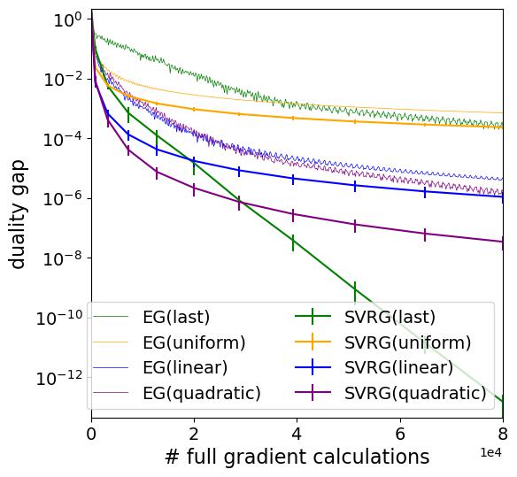
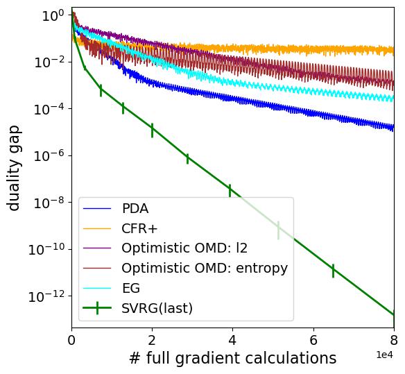
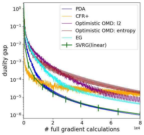
Figure 1: Numerical results on policeman and burglar game. Random algorithms are implemented with seeds 0-9. We draw plots with error bars representing standard deviations across different seeds. The y-axis shows performance in terms of the duality gap. The x-axis shows units of computation in terms of the number of evaluations of $F$ (full gradient calculations). The left plot compares SVRG-EG with deterministic EG. The center plot compares the last-iterate behavior of all algorithms. The right plot compares the linear average of all algorithms.

In all cases, we see that the SVRG-EG algorithm outperforms deterministic EG, no matter whether we look at last iterate, uniform, linear, or quadratic iterate averaging. In the policeman and burglar problem, the last iterates of SVRG-EG show a linear convergence rate, unlike any other method. In random matrix game, linear and quadratic iterate averaging performs best, and SVRG-EG with linear averaging beats every method except CFR+.

Extensive-form games

We also evaluate the numerical performance of SVRG-EG on extensive-form games, which can be cast as bilinear saddle-point problems similar to Equation 11 using the sequence-form representation [49]. Instead of a simplex, the feasible region of EFGs is describled by the treeplex, which is generalization of simplexes that captures the sequential structure of an EFG [17].

We test the EG methods on the Leduc poker game [45] and the Search game from Kroer et al. [26]. As before, we use the same oracle such that Assumption $4$ holds with $L=\lVert A\rVert_{F}$. The results on Search are in Figure 2, while the results on Leduc are deferred to Section E.2.

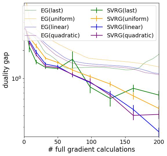
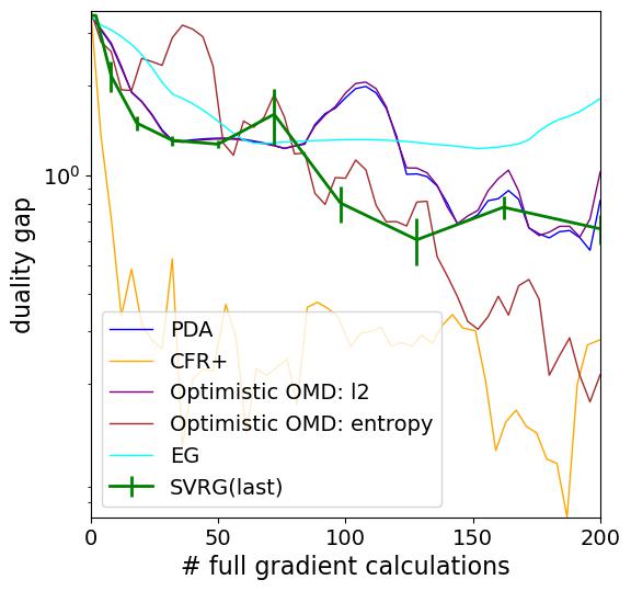
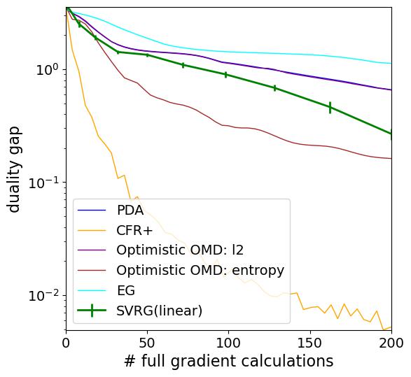
Figure 2: Numerical results on Search (zero sum) game. Random algorithms are implemented with seeds 0-9. The setup is the same as in Figure 1.

In Search, the SVRG-EG algorithms outperform EG. For Leduc in the appendix, we find that SVRG-EG and EG are very similar. This is likely because the payoff matrices $A$ in EFGs are more sparse, and $\lVert A\rVert_{F}$ is much larger than $\lVert A\rVert_{2}$. Thus, the theoretical stepsizes for SVRG-EG are much smaller, which makes them converge slowly. IIAS again leads to much better performance than uniform iterate averaging. In both cases, though, SVRG-EG is still not competitive with CFR+. It is an interesting future direction to design better gradient estimators or adaptive stepsize schemes for improving the performance of SVRG-EG to be competitive with CFR+.

Image segmentation

Image segmentation is a process of dividing an $m\times n$ image into a collection of $h$ regions of pixels such that each region is homogenerous, while the total interface between the regions is minimized. It is essential in image analysis and pattern recognition, and generally difficult [11, 9]. Chambolle and Pock [7] showed that under the assumption that the optimal centroids of regions are known, the partitioning problem can be formulated as a SPP of the form:

$$\min_{u:u_{ij\cdot}\in\Delta^{h}}\max_{v:{\lVert v_{ij\cdot}\rVert}_{\infty}\leq\frac{1}{2}}\sum_{l=1}^{h}\left(u_{\cdot\cdot l}^{T}Av_{\cdot\cdot l}+\langle d_{\cdot\cdot l},u_{\cdot\cdot l}\rangle\right),$$ (12)

where $u$ and $v$ are $mnh$ and $2mnh$ dimensional vectors, respectively. $A\in\{-1,0,1\}^{mn\times mn}$ and $d\in\mathbb{R}^{mnh}$. This is a non-strongly convex-concave SPP satisfying the condition in Theorem 4, and thus the error-bound condition. We run the SVRG-EG algorithm and other Euclidean-distance-based deterministic methods on this problem (the remaining algorithms are not applicable to the dual domain). We show an image instance in Figure 3, while leaving other results to the appendix. SVRG-EG significantly outperforms all other methods with linear averaging and in last iterate (last iterate plots are in Section E.2).

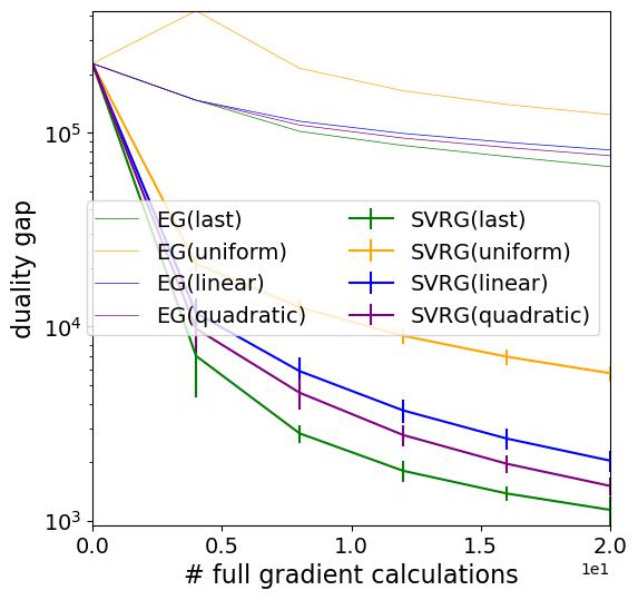
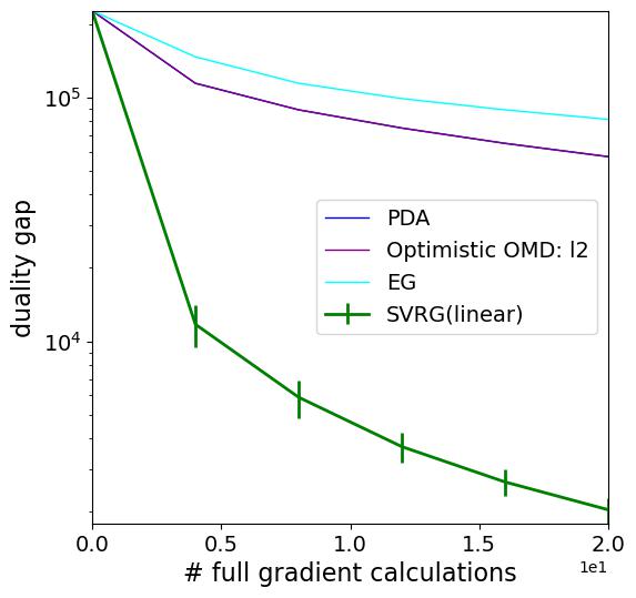
Figure 3: An image segmentation instance. Top left is the original image. Top right is the segmentation result from solving Equation 12 via SVRG-EG. Bottom left is numerical performance of SVRG-EG compared to EG. Random algorithms are implemented with seeds 0-5. Other setups are the same as in Figure 1. Bottom right is the numerical performance for all applicable algorithms, with linear averaging. Note that PDA and Optimistic OMD overlap.

 

Supplementary Materials for
Convergence of SVRG-Extragradient for Variational Inequalities: Error Bounds and Increasing Iterate Averaging

 

Appendix A ADDITIONAL RELATED WORK

Variance reduction.

There is a huge literature on variance reduction techniques in stochastic optimization. Johnson and Zhang [21] is a seminal work in the context of stochastic gradient descent for finite-sum minimization, mainly motivated by supervised learning settings. Via relatively simple analysis, the authors showed that SVRG ensures linear convergence when the minimization problem is smooth and strongly convex. Roux et al. [43], Schmidt et al. [44] considered closely related stochastic averaging gradient (SAG) methods and established their sublinear and linear convergence rates for general convex and strongly convex, smooth problems, respectively. Defazio et al. [10] proposed SAGA, an incremental gradient algorithm that combines algorithmic ideas in SVRG and SAG. The authors showed that they can all be derived from a variance reduction approach, using different gradient and function value estimates, but SAGA achieves a faster linear convergence rate for strongly convex problems. Kovalev et al. [25] introduced the loopless SVRG variant for convex minimization and showed linear convergence.

Recent work on stochastic extragradient.

There is also recent literature on stochastic (non-SVRG) extragradient methods for saddle-point problems where finite-sum structure and variance reduction are not considered [28, 13, 29]. There, the problem settings and types of guarantees are very different from the ones we consider in this work. In particular, none of them allow polyhedral feasible sets, such as strategy sets of EFGs.

Appendix B LINEAR CONVERGENCE ANALYSIS FOR SVRG-EG

B.1 Proofs of Lemmas

Proof of Lemma 1

Proof.

The error-bound condition (5) tells us that there exist scalars $\epsilon_{0}>0$ and $C_{0}>0$ such that

$$\min_{z^{*}\in\mathcal{Z}^{*}}\left\lVert z-z^{*}\right\rVert\leq\frac{C_{0}}{\tau}\left\lVert z-\Pi_{\mathcal{Z}}(z-\tau F(z))\right\rVert$$ (13)

for all $z\in\mathcal{Z}$ such that $\lVert z-\Pi_{\mathcal{Z}}(z-\tau F(z))\rVert\leq\tau\epsilon_{0}$.

Obviously, for $z\in\mathcal{Z}$ such that $\lVert z-\Pi_{\mathcal{Z}}(z-\tau F(z))\rVert>\tau\epsilon_{0}$, we have

$$\lVert z-\Pi_{\mathcal{Z}^{*}}(z)\rVert\leq D(\mathcal{Z})=\frac{D(\mathcal{Z})}{\tau\epsilon_{0}}\tau\epsilon_{0}<\frac{D(\mathcal{Z})}{\tau\epsilon_{0}}\lVert z-\Pi_{\mathcal{Z}}(z-\tau F(z))\rVert,$$ (14)

where $D(\mathcal{Z})=\max_{z,z^{\prime}\in\mathcal{Z}}\lVert z-z^{\prime}\rVert$.

Let $C=\max\left\{\frac{C_{0}}{\tau},\frac{D(\mathcal{Z})}{\tau\epsilon_{0}}\right\}$. Consequently, for all $z\in\mathcal{Z}$, the inequality $\min_{z^{*}\in\mathcal{Z}^{*}}\left\lVert z-z^{*}\right\rVert\leq C\left\lVert z-\Pi_{\mathcal{Z}}(z-\tau F(z))\right\rVert$ holds. This completes the proof of the lemma. ∎

Proof of Lemma 2

Proof.

To prove this lemma, we introduce a sequence of auxiliary “quasi $(k+\frac{1}{2})$th iterates”: for each $k$, denote $\tilde{z}_{k+1/2}=\Pi_{\mathcal{Z}}(\bar{z}_{k}-\tau F(\bar{z}_{k}))$, which is the standard update of the first step of the deterministic EG starting from $\bar{z}_{k}$ (using $F(\bar{z}_{k})$ instead of $F(w_{k})$). Intuitively, we show that $z_{k+1/2}$ is an approximation of $\tilde{z}_{k+1/2}$ when $\tau$ is small, while $\tilde{z}_{k+1/2}$ satisfies the error bound condition as in the classical analysis of deterministic EG. As such, error bounds (on $\bar{z}_{k}$) still hold.

To bound the distance between $\tilde{z}_{k+1/2}$ and $z_{k+1/2}$, we use non-expansiveness of projection operator $\Pi_{\mathcal{Z}}$:

$$\lVert\tilde{z}_{k+1/2}-z_{k+1/2}\rVert=\lVert\Pi_{\mathcal{Z}}(\bar{z}_{k}-\tau F(\bar{z}_{k}))-\Pi_{\mathcal{Z}}(\bar{z}_{k}- \tau F(w_{k}))\rVert\leq\tau\lVert F(\bar{z}_{k})-F(w_{k})\rVert$$

$$\leq\tau L\lVert\bar{z}_{k}-w_{k}\rVert=\alpha\tau L\lVert z_{k}-w_{k}\rVert.$$ (15)

The second inequality follows from the fact that the operator $F$ is also $L$-Lipschitz since $\lVert F(z_{1})-F(z_{2})\rVert^{2}=\lVert\mathbb{E}_{\xi}[F_{\xi}(z_{1})-F_{\xi}(z_{2})]\rVert\leq\mathbb{E}_{\xi}\lVert F_{\xi}(z_{1})-F_{\xi}(z_{2})\rVert^{2}\leq L^{2}\lVert z_{1}-z_{2}\rVert^{2},\;\forall z_{1},z_{2}\in\mathcal{Z}$.

With Equation 15, we can bound $\lVert\bar{z}_{k}-\tilde{z}_{k+1/2}\rVert^{2}$ as

$$\lVert\bar{z}_{k}-\tilde{z}_{k+1/2}\rVert^{2}$$

$$\leq 2\lVert\bar{z}_{k}-z_{k+1/2}\rVert^{2}+2\lVert\tilde{z}_{k+1/2}-z_{k+1/2}\rVert^{2}$$

$$\leq 2\alpha\lVert z_{k}-z_{k+1/2}\rVert^{2}+2(1-\alpha)\lVert w_{k}-z_{k+1/2}\rVert^{2}-2\alpha(1-\alpha)\lVert z_{k}-w_{k}\rVert^{2}+2\alpha^{2}\tau^{2}L^{2}\lVert z_{k}-w_{k}\rVert^{2}$$

$$= 2\alpha\lVert z_{k}-z_{k+1/2}\rVert^{2}+2(1-\alpha)\lVert w_{k}-z_{k+1/2}\rVert^{2}+2\alpha\left(\alpha\tau^{2}L^{2}-(1-\alpha)\right)\lVert z_{k}-w_{k}\rVert^{2},$$ (16)

where we use $\lVert a+b\rVert^{2}\leq 2\lVert a\rVert^{2}+2\lVert b\rVert^{2}$, $\lVert\alpha a+(1-\alpha)b\rVert^{2}=\alpha\lVert a\rVert^{2}+(1-\alpha)\lVert b\rVert^{2}-\alpha(1-\alpha)\lVert a-b\rVert^{2}$ and Equation 15.

On the other hand, we have

$$\lVert\bar{z}_{k}-\Pi_{\mathcal{Z}^{*}}(\bar{z}_{k})\rVert^{2}\geq\frac{1}{2}\lVert z_{k}-\Pi_{\mathcal{Z}^{*}}(\bar{z}_{k})\rVert^{2}-\lVert\bar{z}_{k}-z_{k}\rVert^{2}=\frac{1}{2}\lVert z_{k}-\Pi_{\mathcal{Z}^{*}}(\bar{z}_{k})\rVert^{2}-(1-\alpha)^{2}\lVert z_{k}-w_{k}\rVert^{2}$$ (17)

and

$$\lVert\bar{z}_{k}-\Pi_{\mathcal{Z}^{*}}(\bar{z}_{k})\rVert^{2}\geq\frac{1}{2}\lVert w_{k}-\Pi_{\mathcal{Z}^{*}}(\bar{z}_{k})\rVert^{2}-\lVert\bar{z}_{k}-w_{k}\rVert^{2}=\frac{1}{2}\lVert w_{k}-\Pi_{\mathcal{Z}^{*}}(\bar{z}_{k})\rVert^{2}-\alpha^{2}\lVert z_{k}-w_{k}\rVert^{2}.$$ (18)

Combining Equations 17 and 18 with a weight coefficient $\theta$, we obtain

$$\lVert\bar{z}_{k}-\Pi_{\mathcal{Z}^{*}}(\bar{z}_{k})\rVert^{2} =\theta\lVert\bar{z}_{k}-\Pi_{\mathcal{Z}^{*}}(\bar{z}_{k})\rVert^{2}+(1-\theta)\lVert\bar{z}_{k}-\Pi_{\mathcal{Z}^{*}}(\bar{z}_{k})\rVert^{2}$$

$$\geq\frac{1}{2}\Phi^{\theta}_{\Pi_{\mathcal{Z}^{*}}(\bar{z}_{k})}(z_{k},w_{k})-\left(\theta(1-\alpha)^{2}+(1-\theta)\alpha^{2}\right)\lVert z_{k}-w_{k}\rVert^{2}$$

$$\geq\frac{1}{2}\textnormal{dist}^{\theta}_{\mathcal{Z}^{*}}(z_{k},w_{k})-\left(\theta(1-\alpha)^{2}+(1-\theta)\alpha^{2}\right)\lVert z_{k}-w_{k}\rVert^{2},$$ (19)

where the last inequality follows from the definition of $\textnormal{dist}^{\theta}_{\mathcal{Z}^{*}}(z_{k},w_{k})$.

By applying Lemma 1, it follows that

$$\lVert\bar{z}_{k}-\Pi_{\mathcal{Z}^{*}}(\bar{z}_{k})\rVert^{2}\leq C^{2}\lVert\bar{z}_{k}-\tilde{z}_{k+1/2}\rVert^{2}.$$ (20)

Combining this with Equations 16 and 19, and using $C=\frac{\bar{C}}{\tau}$, we obtain that

$$\frac{1}{2}\textnormal{dist}^{\theta}_{\mathcal{Z}^{*}}(z_{k},w_{k})-\left(\theta(1-\alpha)^{2}+(1-\theta)\alpha^{2}\right)\lVert z_{k}-w_{k}\rVert^{2}$$

$$\leq \frac{\bar{C}^{2}}{\tau^{2}}\left(2\alpha\lVert z_{k}-z_{k+1/2}\rVert^{2}+2(1-\alpha)\lVert w_{k}-z_{k+1/2}\rVert^{2}+2\alpha\left(\alpha\tau^{2}L^{2}-(1-\alpha)\right)\lVert z_{k}-w_{k}\rVert^{2}\right).$$ (21)

Since $\tau\leq\frac{\sqrt{1-\alpha}}{L}$, we have $\alpha\tau^{2}L^{2}-(1-\alpha)\leq 0$ and therefore

$$\frac{1}{2}\textnormal{dist}^{\theta}_{\mathcal{Z}^{*}}(z_{k},w_{k})-\left(\theta(1-\alpha)^{2}+(1-\theta)\alpha^{2}\right)\lVert z_{k}-w_{k}\rVert^{2}$$

$$\leq \frac{2\bar{C}^{2}}{\tau^{2}}\left(\alpha\lVert z_{k}-z_{k+1/2}\rVert^{2}+(1-\alpha)\lVert w_{k}-z_{k+1/2}\rVert^{2}\right).$$ (22)

Re-arranging terms and using $\theta(1-\alpha)^{2}+(1-\theta)\alpha^{2}\leq 2$, we have

$$\frac{1}{2}\textnormal{dist}^{\theta}_{\mathcal{Z}^{*}}(z_{k},w_{k})\leq\frac{2\bar{C}^{2}}{\tau^{2}}\left(\alpha\lVert z_{k}-z_{k+1/2}\rVert^{2}+(1-\alpha)\lVert w_{k}-z_{k+1/2}\rVert^{2}\right)+2\lVert z_{k}-w_{k}\rVert^{2}.$$ (23)

Then, we bound the last term in the above inequality as follows:

$$2\lVert z_{k}-w_{k}\rVert^{2} \leq 4\lVert z_{k}-z_{k+1/2}\rVert^{2}+4\lVert w_{k}-z_{k+1/2}\rVert^{2}$$

$$=\frac{4}{\tau^{2}}\left(\tau^{2}\lVert z_{k}-z_{k+1/2}\rVert^{2}+\tau^{2}\lVert w_{k}-z_{k+1/2}\rVert^{2}\right)$$

$$\leq\frac{4}{\tau^{2}}\left(\frac{1-\alpha}{L^{2}}\lVert z_{k}-z_{k+1/2}\rVert^{2}+\frac{1-\alpha}{L^{2}}\lVert w_{k}-z_{k+1/2}\rVert^{2}\right)$$

$$\leq\frac{4}{\tau^{2}L^{2}}\left(\lVert z_{k}-z_{k+1/2}\rVert^{2}+(1-\alpha)\lVert w_{k}-z_{k+1/2}\rVert^{2}\right)$$

$$\leq\frac{4}{\tau^{2}\alpha L^{2}}\left(\alpha\lVert z_{k}-z_{k+1/2}\rVert^{2}+(1-\alpha)\lVert w_{k}-z_{k+1/2}\rVert^{2}\right).$$ (24)

This yields that

$$\frac{1}{2}\textnormal{dist}^{\theta}_{\mathcal{Z}^{*}}(z_{k},w_{k})\leq\left(\frac{2\bar{C}^{2}}{\tau^{2}}+\frac{4}{\alpha L^{2}\tau^{2}}\right)\left(\alpha\lVert z_{k}-z_{k+1/2}\rVert^{2}+(1-\alpha)\lVert w_{k}-z_{k+1/2}\rVert^{2}\right).$$ (25)

Equivalently,

$$\tau^{2}\frac{\alpha L^{2}}{4\alpha\bar{C}^{2}L^{2}+8}\textnormal{dist}^{\theta}_{\mathcal{Z}^{*}}(z_{k},w_{k})\leq\alpha\lVert z_{k}-z_{k+1/2}\rVert^{2}+(1-\alpha)\lVert w_{k}-z_{k+1/2}\rVert^{2}.$$ (26)

Since $\frac{\gamma\sqrt{1-\alpha}}{L}\leq\frac{\sqrt{1-\alpha}}{L}$, Equation 3 holds.

∎

B.2 Loopless SVRG-EG Proofs

Proof of Theorem 1

Proof.

First, to make our work self-contained, we derive here a crucial inequality, which is similar to Alacaoglu and Malitsky [1, Equation (10)].

For brevity, let $\hat{F}(z_{k+1/2})=F(w)+F_{\xi_{k}}(z_{k+1/2})-F_{\xi_{k}}(w)$. By the property of the proximal mapping and the definitions of $z_{k+1}$ and $z_{k+1/2}$, we have, for all $z$,

$$\langle z_{k+1}-\bar{z}_{k}+\tau\hat{F}(z_{k+1/2}),z-z_{k+1}\rangle\geq 0,$$ (27)

$$\langle z_{k+1/2}-\bar{z}_{k}+\tau F(w),z_{k+1}-z_{k+1/2}\rangle\geq 0$$ (28)

for any $k=0,1,\ldots$. We sum up these two inequalities, and rearrange terms to obtain

$$\langle z_{k+1}-\bar{z}_{k},\,z-z_{k+1}\rangle+\langle z_{k+1/2}-\bar{z}_{k},\,z_{k+1}-z_{k+1/2}\rangle$$

$$\hskip 60.0pt+\tau\langle F_{\xi_{k}}(w_{k})-F_{\xi_{k}}(z_{k+1/2}),\,z_{k+1}-z_{k+1/2}\rangle+\tau\langle\hat{F}(z_{k+1/2}),\,z-z_{k+1/2}\rangle\geq 0.$$ (29)

To bound the inner products we use the definition of $\bar{z}^{s}_{k}$ and the identity $2\langle a,\,b\rangle={\lVert a+b\rVert}^{2}-{\lVert a\rVert}^{2}-{\lVert b\rVert}^{2}$:

$$2\langle z_{k+1}-\bar{z}_{k},z-z_{k+1}\rangle=\alpha{\lVert z_{k}-z\rVert}^{2} -{\lVert z_{k+1}-z\rVert}^{2}+(1-\alpha){\lVert w_{k}-z\rVert}^{2}$$

$$-\alpha{\lVert z_{k+1}-z_{k}\rVert}^{2}-(1-\alpha){\lVert z_{k+1}-w_{k}\rVert}^{2},$$ (30)

$$2\langle z_{k+1/2}-\bar{z}_{k},\,z_{k+1}-z_{k+1/2}\rangle =\alpha{\lVert z_{k+1}-z_{k}\rVert}^{2}-{\lVert z_{k+1}-z_{k+1/2}\rVert}^{2}+(1-\alpha){\lVert z_{k+1}-w_{k}\rVert}^{2}$$

$$\hskip 20.0pt-\alpha{\lVert z_{k+1/2}-z_{k}\rVert}^{2}-(1-\alpha){\lVert z_{k+1/2}-w_{k}\rVert}^{2}.$$ (31)

Next, we bound the last two terms in Equation 29.

$$\mathbb{E}_{k}[2\tau\langle F_{\xi_{k}}(w_{k})-F_{\xi_{k}}(z_{k+1/2}),\,z_{k+1}-z_{k+1/2}\rangle]$$

$$\leq \mathbb{E}_{k}[2\tau\lVert F_{\xi_{k}}(w_{k})-F_{\xi_{k}}(z_{k+1/2})\rVert\cdot\lVert z_{k+1}-z_{k+1/2}\rVert]$$

$$\leq \mathbb{E}_{k}\left[\frac{\tau^{2}}{\gamma}{\lVert F_{\xi_{k}}(w_{k})-F_{\xi_{k}}(z_{k+1/2})\rVert}^{2}+\gamma{\lVert z_{k+1}-z_{k+1/2}\rVert}^{2}\right]$$

$$= \frac{\tau^{2}}{\gamma}\mathbb{E}_{k}{\lVert F_{\xi_{k}}(w_{k})-F_{\xi_{k}}(z_{k+1/2})\rVert}^{2}+\gamma\mathbb{E}_{k}{\lVert z_{k+1}-z_{k+1/2}\rVert}^{2}$$

$$\leq \frac{\tau^{2}L^{2}}{\gamma}\lVert w_{k}-z_{k+1/2}\rVert^{2}+\gamma\mathbb{E}_{k}{\lVert z_{k+1}-z_{k+1/2}\rVert}^{2},$$ (32)

where the last inequality follows from the $L$-Lipschitz continuity of $F_{\xi}$.

Let $z=z^{*}\in\mathcal{Z}^{*}$. By the monotonicity of $F$ and the definition of (VI), we have

$$\mathbb{E}_{k}\left[\langle\hat{F}(z_{k+1/2}),\,z^{*}-z_{k+1/2}\rangle\right]=-\langle F(z_{k+1/2}),\,z_{k+1/2}-z^{*}\rangle\leq-\langle F(z^{*}),z_{k+1/2}-z^{*}\rangle\leq 0.$$ (33)

Therefore, combining Equations 29, 30, 31, 32 and 33, we obtain

$$\mathbb{E}_{k}[\lVert z_{k+1}-z^{*}\rVert^{2}]\leq \alpha{\lVert z_{k}-z^{*}\rVert}^{2}+(1-\alpha){\lVert w_{k}-z^{*}\rVert}^{2}$$

$$-\left((1-\alpha)-\frac{\tau^{2}L^{2}}{\gamma}\right){\lVert w_{k}-z_{k+1/2}\rVert}^{2}-\alpha\lVert z_{k}-z_{k+1/2}\rVert^{2}.$$ (34)

By the definition of $w_{k+1/2}$,

$$\mathbb{E}_{k+1/2}\lVert w_{k+1}-z\rVert^{2}=p\lVert z_{k+1}-z\rVert^{2}+(1-p)\lVert w_{k}-z\rVert^{2}\quad\forall\,z\in\mathcal{Z}.$$ (35)

By the tower property $\mathbb{E}_{k}[\mathbb{E}_{k+1/2}[\cdot]]=\mathbb{E}_{k}[\cdot]$ and letting $z=z^{*}$, it follows that

$$\mathbb{E}_{k}\lVert w_{k+1}-z^{*}\rVert^{2}=p\mathbb{E}_{k}\lVert z_{k+1}-z^{*}\rVert^{2}+(1-p)\lVert w_{k}-z^{*}\rVert^{2}$$ (36)

and hence

$$\frac{1-\alpha}{p}\mathbb{E}_{k}\lVert w_{k+1}-z^{*}\rVert^{2}=(1-\alpha)\mathbb{E}_{k}\lVert z_{k+1}-z^{*}\rVert^{2}+\frac{(1-\alpha)(1-p)}{p}\lVert w_{k}-z^{*}\rVert^{2}.$$ (37)

We plug Equation 37 into Equation 34 and then attain that

$$\mathbb{E}_{k}\left(\alpha{\lVert z_{k+1}-z^{*}\rVert}^{2}+\frac{1-\alpha}{p}{\lVert w_{k+1}-z^{*}\rVert}^{2}\right)$$

$$\leq \alpha{\lVert z_{k}-z^{*}\rVert}^{2}+\frac{1-\alpha}{p}{\lVert w_{k}-z^{*}\rVert}^{2}-\left((1-\alpha)-\frac{\tau^{2}L^{2}}{\gamma}\right)\lVert w_{k}-z_{k+1/2}\rVert^{2}-\alpha\lVert z_{k}-z_{k+1/2}\rVert^{2}.$$ (38)

Since $\tau\leq\frac{\gamma\sqrt{1-\alpha}}{L}$, we can conclude that

$$\mathbb{E}_{k}\left(\alpha{\lVert z_{k+1}-z^{*}\rVert}^{2}+\frac{1-\alpha}{p}{\lVert w_{k+1}-z^{*}\rVert}^{2}\right)$$

$$\leq \alpha{\lVert z_{k}-z^{*}\rVert}^{2}+\frac{1-\alpha}{p}{\lVert w_{k}-z^{*}\rVert}^{2}-(1-\gamma)(1-\alpha)\lVert w_{k}-z_{k+1/2}\rVert^{2}-\alpha\lVert z_{k}-z_{k+1/2}\rVert^{2}.$$ (39)

Let $\tilde{\theta}=\frac{\alpha}{\alpha+\frac{1-\alpha}{p}}$. Then,

$$\left(\alpha+\frac{1-\alpha}{p}\right)\Phi^{\tilde{\theta}}_{z^{*}}(z_{k},w_{k})=\alpha{\lVert z_{k}-z^{*}\rVert}^{2}+\frac{1-\alpha}{p}{\lVert w_{k}-z^{*}\rVert}^{2}.$$ (40)

Using the notation of Equation 40 and $\gamma\in(0,1)$, we can transform Equation 39 into

$$\left(\alpha+\frac{1-\alpha}{p}\right)\mathbb{E}_{k}\Phi^{\tilde{\theta}}_{z^{*}}(z_{k+1},w_{k+1})\leq \left(\alpha+\frac{1-\alpha}{p}\right)\Phi^{\tilde{\theta}}_{z^{*}}(z_{k},w_{k})$$

$$-(1-\gamma)\left(\alpha\lVert z_{k}-z_{k+1/2}\rVert^{2}+(1-\alpha)\lVert w_{k}-z_{k+1/2}\rVert^{2}\right).$$ (41)

Applying Lemma 2 with $\theta=\tilde{\theta}$ in Equation 41, we have

$$\left(\alpha+\frac{1-\alpha}{p}\right)\mathbb{E}_{k}\Phi^{\tilde{\theta}}_{z^{*}}(z_{k+1},w_{k+1})$$

$$\leq \left(\alpha+\frac{1-\alpha}{p}\right)\Phi^{\tilde{\theta}}_{z^{*}}(z_{k},w_{k})-(1-\gamma)\left(\alpha\lVert z_{k}-z_{k+1/2}\rVert^{2}+(1-\alpha)\lVert w_{k}-z_{k+1/2}\rVert^{2}\right)$$

$$\leq \left(\alpha+\frac{1-\alpha}{p}\right)\Phi^{\tilde{\theta}}_{z^{*}}(z_{k},w_{k})-\tau^{2}\frac{(1-\gamma)\alpha L^{2}}{4\alpha\bar{C}^{2}L^{2}+8}\textnormal{dist}^{\tilde{\theta}}_{\mathcal{Z}^{*}}(z_{k},w_{k}).$$ (42)

Let $z^{*}=\Pi^{\tilde{\theta}}_{\mathcal{Z}}(z_{k},w_{k})$, then $\Phi^{\tilde{\theta}}_{z^{*}}(z_{k},w_{k})=\textnormal{dist}^{\theta}_{\mathcal{Z}^{*}}(z_{k},w_{k})$ and thus

$$\mathbb{E}_{k}\Phi^{\tilde{\theta}}_{z^{*}}(z_{k+1},w_{k+1})\leq \left(1-\tau^{2}\frac{(1-\gamma)\alpha L^{2}}{\left(4\alpha\bar{C}^{2}L^{2}+8\right)\left(\alpha+\frac{1-\alpha}{p}\right)}\right)\textnormal{dist}^{\tilde{\theta}}_{\mathcal{Z}^{*}}(z_{k},w_{k}).$$ (43)

By the definition of $\textnormal{dist}^{\tilde{\theta}}_{\mathcal{Z}^{*}}(z_{k+1},w_{k+1})$, we complete the proof by

$$\mathbb{E}_{k}\textnormal{dist}^{\tilde{\theta}}_{\mathcal{Z}^{*}}(z_{k+1},w_{k+1})\leq \mathbb{E}_{k}\Phi^{\tilde{\theta}}_{z^{*}}(z_{k+1},w_{k+1})$$

$$\leq \left(1-\tau^{2}\frac{(1-\gamma)\alpha L^{2}}{\left(4\alpha\bar{C}^{2}L^{2}+8\right)\left(\alpha+\frac{1-\alpha}{p}\right)}\right)\textnormal{dist}^{\tilde{\theta}}_{\mathcal{Z}^{*}}(z_{k},w_{k}).$$ (44)

∎

Proof of Corollary 1

Proof.

Let

$$\rho=\tau^{2}\frac{(1-\gamma)\alpha L^{2}}{\left(4\alpha\bar{C}^{2}L^{2}+8\right)\left(\alpha+\frac{1-\alpha}{p}\right)}.$$

By iterating Theorem 1 and taking the total expectation $\mathbb{E}_{0}$, we have

$$\mathbb{E}_{0}\left[\textnormal{dist}^{\tilde{\theta}}_{\mathcal{Z}^{*}}(z_{k},w_{k})\right]\leq(1-\rho)^{k}\textnormal{dist}^{\tilde{\theta}}_{\mathcal{Z}^{*}}(z_{0},w_{0})=(1-\rho)^{k}\min_{z^{*}\in\mathcal{Z}^{*}}\lVert z_{0}-z^{*}\rVert^{2}.$$ (45)

To reach expected $\epsilon$-accuracy as measured by the weighted distance (Lyapunov function) to the solution set, we need $(1-\rho)^{k}\leq\epsilon$ and equivalently,

$$k\geq\frac{1}{\mathop{{\rm log}}{\frac{1}{1-\rho}}}\mathop{{\rm log}}{\frac{1}{\epsilon}}\approx\frac{1}{\rho}\mathop{{\rm log}}{\frac{1}{\epsilon}}\quad\text{when $\rho$ is small},$$ (46)

where $k$ counts the number of iterations.

Recall that $1-\alpha=p=\frac{2}{N}$, $\gamma=0.99$ and $\tau=\frac{0.99\sqrt{2}}{\sqrt{N}L}$. Since

$$\frac{1}{\rho}=\frac{\left(4\alpha\bar{C}^{2}L^{2}+8\right)\left(\alpha+\frac{1-\alpha}{p}\right)}{(1-\gamma)\tau^{2}\alpha L^{2}}=\frac{\left(4(1-\frac{2}{N})\bar{C}^{2}L^{2}+8\right)\left(2-\frac{2}{N}\right)}{0.01\times\frac{0.99^{2}\times 2}{NL^{2}}\times(1-\frac{2}{N})L^{2}}={\cal O}(\bar{C}^{2}NL^{2}+N).$$ (47)

Since we need $2+pN$ evaluations of $F_{\xi}$ per iteration, we need $4\times k$ evaluations of $F_{\xi}$ to reach expected $\epsilon$-accuracy. Therefore, we attain that the time complexity is $\mathcal{O}\left((\bar{C}^{2}NL^{2}+N)\mathop{{\rm log}}{\frac{1}{\epsilon}}\right)$. ∎

B.3 Double-loop SVRG-EG

Here, we formally introduce the double-loop version of the SVRG-EG algorithm:

Input: Set the inner loop iteration $K$, probability distribution $Q$, step size $\tau$, $\alpha\in(0,1)$, $z^{0}_{0}=w^{0}=z_{0}$

for $s=0,1,\cdots$ do

       for $k=0,1,\cdots,K-1$ do

             $\bar{z}^{s}_{k}=\alpha z^{s}_{k}+(1-\alpha)w^{s}$;

             $z^{s}_{k+1/2}=\mathop{\rm Prox}_{\tau g}(\bar{z}^{s}_{k}-\tau F(w^{s}))$;

             Draw an index $\xi^{s}_{k}$ according to $Q$;

             $z^{s}_{k+1}=\mathop{\rm Prox}_{\tau g}\left(\bar{z}^{s}_{k}-\tau[F(w^{s})+F_{\xi^{s}_{k}}(z^{s}_{k+1/2})-F_{\xi^{s}_{k}}(w^{s})]\right)$;

            

       end for

      $w^{s}=\frac{1}{K}\sum_{k=1}^{K}z^{s}_{k}$;

       $z^{s+1}_{0}=z^{s}_{k}$;

      

end for

Algorithm 2 Double-loop SVRG-Extragradient (D-SVRG-EG)

In the double-loop SVRG-Extragradient algorithm, the reference points are updated once per outer iteration instead of the stochastic updates in the (loopless) SVRG-EG. Also, the reference points are computed based on averaging over all generated points in the previous inner loop, instead of the last iterate in (loopless) SVRG-EG.

For the double-loop SVRG-EG algorithm, we prove the following linear convergence guarantee and corresponding time complexity.

Analogously, we define a Lyapunov function

$$\textnormal{dist}^{\theta}_{\mathcal{Z}^{*}}(z^{s}_{0},w^{s})=\min_{z^{*}\in\mathcal{Z}^{*}}\theta\lVert z^{s}_{0}-z^{*}\rVert^{2}+(1-\theta)\lVert w^{s}-z^{*}\rVert^{2}.$$ (48)

Theorem 5.

Assume Assumptions $1$-$4$ and Error-Bound Condition hold. Let $\{z^{s}_{k},w^{s}\}_{s\in\mathbb{N}_{+},k=0,\ldots,K-1}$ be iterates generated by Algorithm 2 with $K\in\mathbb{N}_{+}$, $\alpha\in[0,1),\tau=\gamma\frac{\sqrt{1-\alpha}}{L}$, for $\gamma\in(0,1)$. Then, we have

$$\mathbb{E}^{s}_{0}\left[\textnormal{dist}^{\theta}_{\mathcal{Z}^{*}}(z^{s+1}_{0},w^{s+1})\right]\leq\left(1-\frac{(1-\gamma)K}{16\tilde{C}^{2}(\alpha+K(1-\alpha))}\right)^{s}\textnormal{dist}^{\theta}_{\mathcal{Z}^{*}}(z^{s}_{0},w^{s}),$$ (49)

where $\theta=\frac{\alpha}{\alpha+K(1-\alpha)}$ and $\tilde{C}=\max\left\{\frac{\bar{C}}{\tau},\sqrt{\frac{4K+2}{\alpha(1-\alpha)}}\right\}$.

Corollary 4.

Let $K=\frac{N}{2}$, $\alpha=1-\frac{2}{N}$ and $\tau=\frac{0.99\sqrt{2}}{\sqrt{N}L}$ in Algorithm 2. Then, the time complexity to reach $\epsilon$-accuracy is $\mathcal{O}\left(\left(\bar{C}^{2}NL^{2}+N^{2}\right)\mathop{{\rm log}}{\frac{1}{\epsilon}}\right)$.

Remarks.

We show that the double-loop SVRG-EG exhibits a linear convergence rate of the same magnitude (in terms of its dependence on $N$) as its loopless counterpart in the typical case where $\bar{C}^{2}L^{2}\gg 1$.

Lemma of error-bound condition for double-loop SVRG-EG

To prove the linear convergence of double-loop SVRG-EG, we need a “new” Lemma 2. We state this lemma as follows.

Lemma 6.

Assume Assumptions $1$-$4$ and Error-Bound Condition hold. Let $K\in\mathbb{N}_{+}$, $\alpha\in[0,1),\tau=\gamma\frac{\sqrt{1-\alpha}}{L}$, for $\gamma\in(0,1)$, and $\theta\in[0,1]$. Then, for $s\geq 1$,  Algorithm 2 ensures

$$\frac{K}{8\tilde{C}^{2}}\textnormal{dist}^{\theta}_{\mathcal{Z}^{*}}(z^{s}_{0},w^{s})\leq\mathbb{E}^{s}_{0}\left[\sum_{k=0}^{K-1}\left(\alpha\lVert z^{s}_{k+1/2}-z^{s}_{k}\rVert^{2}+(1-\alpha)\lVert z^{s}_{k+1/2}-w^{s}\rVert^{2}\right)\right]+e^{s},$$ (50)

where $\tilde{C}\geq\frac{\bar{C}^{2}}{\tau^{2}}$, and

$$e^{s}=\frac{1}{\tilde{C}^{2}}\sum_{k=0}^{K-1}\mathbb{E}^{s}_{0}\lVert z^{s}_{k}-w^{s}\rVert^{2}+\frac{5K}{4\tilde{C}^{2}}\lVert z^{s}_{0}-w^{s}\rVert^{2}.$$

Proof.

Let $\tilde{z}^{s}_{k+1/2}=\Pi_{\mathcal{Z}}(\bar{z}^{s}_{k}-\tau F(\bar{z}^{s}_{k}))$ denote a “quasi $(k+\frac{1}{2})$th iterate” in the $s$th epoch. Again, this is not computed by the algorithm, but a variant of $z^{s}_{k+1/2}$ computed using $F(\bar{z}^{s}_{k})$ instead of $F(w^{s})$. To measure the distance between $\tilde{z}^{s}_{k+1/2}$ and $z^{s}_{k+1/2}$, we have

$$\lVert\tilde{z}^{s}_{k+1/2}-z^{s}_{k+1/2}\rVert =\lVert\Pi_{\mathcal{Z}}(\bar{z}^{s}_{k}-\tau F(\bar{z}^{s}_{k}))-\Pi_{\mathcal{Z}}(\bar{z}^{s}_{k}-\tau F(w^{s}))\rVert$$

$$\leq\tau\lVert F(\bar{z}^{s}_{k})-F(w^{s})\rVert$$

$$\leq\tau L\lVert\bar{z}^{s}_{k}-w^{s}\rVert$$

$$=\alpha\tau L\lVert z^{s}_{k}-w^{s}\rVert.$$ (51)

Using Equation 51, we have

$$\lVert\bar{z}^{s}_{k}-\tilde{z}^{s}_{k+1/2}\rVert^{2}$$

$$\leq 2\lVert\bar{z}^{s}_{k}-z^{s}_{k+1/2}\rVert^{2}+2\lVert\tilde{z}^{s}_{k+1/2}-z^{s}_{k+1/2}\rVert^{2}$$

$$= 2\alpha\lVert z^{s}_{k}-z^{s}_{k+1/2}\rVert^{2}+2(1-\alpha)\lVert w^{s}-z^{s}_{k+1/2}\rVert^{2}-2\alpha(1-\alpha)\lVert z^{s}_{k}-w^{s}\rVert^{2}+2\alpha^{2}\tau^{2}L^{2}\lVert z^{s}_{k}-w^{s}\rVert^{2}$$

$$= 2\alpha\lVert z^{s}_{k}-z^{s}_{k+1/2}\rVert^{2}+2(1-\alpha)\lVert w^{s}-z^{s}_{k+1/2}\rVert^{2}+2\alpha\left(\alpha\tau^{2}L^{2}-(1-\alpha)\right)\lVert z^{s}_{k}-w^{s}\rVert^{2},$$ (52)

where we use $\lVert a+b\rVert^{2}\leq 2\lVert a\rVert^{2}+2\lVert b\rVert^{2}$ and $\lVert\gamma a+(1-\gamma)b\rVert^{2}=\gamma\lVert a\rVert^{2}+(1-\gamma)\lVert b\rVert^{2}-\gamma(1-\gamma)\lVert a-b\rVert^{2}$, for $\gamma\in[0,1]$.

On the other hand, by $\lVert a+b\rVert^{2}\leq 2\lVert a\rVert^{2}+2\lVert b\rVert^{2}$ and $\Pi_{\mathcal{Z}^{*}}(z)=\mathop{\rm argmin}_{z^{\prime}\in\mathcal{Z}^{*}}\lVert z-z^{\prime}\rVert$, we have

$$\lVert\bar{z}^{s}_{k}-\Pi_{\mathcal{Z}^{*}}(\bar{z}^{s}_{k})\rVert^{2}\geq \frac{1}{2}\lVert z^{s}_{0}-\Pi_{\mathcal{Z}^{*}}(\bar{z}^{s}_{k})\rVert^{2}-\lVert\bar{z}^{s}_{k}-z^{s}_{0}\rVert^{2}$$

$$\geq \frac{1}{2}\lVert z^{s}_{0}-\Pi_{\mathcal{Z}^{*}}(z^{s}_{0})\rVert^{2}-2\alpha^{2}\lVert z^{s}_{k}-w^{s}\rVert^{2}-2\lVert z^{s}_{0}-w^{s}\rVert^{2}$$ (53)

and

$$\lVert\bar{z}^{s}_{k}-\Pi_{\mathcal{Z}^{*}}(\bar{z}^{s}_{k})\rVert^{2}\geq\frac{1}{2}\lVert w^{s}-\Pi_{\mathcal{Z}^{*}}(\bar{z}^{s}_{k})\rVert^{2}-\lVert\bar{z}^{s}_{k}-w^{s}\rVert^{2}\geq\frac{1}{2}\lVert w^{s}-\Pi_{\mathcal{Z}^{*}}(w^{s})\rVert^{2}-\alpha^{2}\lVert z^{s}_{k}-w^{s}\rVert^{2}.$$ (54)

Combining Equations 53 and 54 with a weight coefficient $\theta$, we obtain

$$\lVert\bar{z}^{s}_{k}-\Pi_{\mathcal{Z}^{*}}(\bar{z}^{s}_{k})\rVert^{2}\geq\frac{\theta}{2}\lVert z^{s}_{0}-\Pi_{\mathcal{Z}^{*}}(z^{s}_{0})\rVert^{2}+\frac{1-\theta}{2}\lVert w^{s}-\Pi_{\mathcal{Z}^{*}}(w^{s})\rVert^{2}-2\theta\lVert z^{s}_{0}-w^{s}\rVert^{2}-(1+\theta)\alpha^{2}\lVert z^{s}_{k}-w^{s}\rVert^{2}.$$ (55)

After summing up Equation 55 over $k=0,\ldots,K-1$ and taking expectation $\mathbb{E}^{s}_{0}$, it follows that

$$\sum_{k=0}^{K-1}\mathbb{E}^{s}_{0}\lVert\bar{z}^{s}_{k}-\Pi_{\mathcal{Z}^{*}}(\bar{z}^{s}_{k})\rVert^{2}$$

$$\geq \frac{K}{2}\theta\lVert z^{s}_{0}-\Pi_{\mathcal{Z}^{*}}(z^{s}_{0})\rVert^{2}+\frac{K}{2}(1-\theta)\lVert w^{s}-\Pi_{\mathcal{Z}^{*}}(w^{s})\rVert^{2}-2\theta K\lVert z^{s}_{0}-w^{s}\rVert^{2}$$

$$\hskip 120.0pt-(1+\theta)\alpha^{2}\sum_{k=0}^{K-1}\mathbb{E}^{s}_{0}\lVert z^{s}_{k}-w^{s}\rVert^{2}$$

$$\geq \frac{K}{4}\theta\lVert z^{s}_{0}-\Pi_{\mathcal{Z}^{*}}(w^{s})\rVert^{2}-\frac{K}{2}\lVert\Pi_{\mathcal{Z}^{*}}(z^{s}_{0})-\Pi_{\mathcal{Z}^{*}}(w^{s})\rVert^{2}+\frac{K}{2}(1-\theta)\lVert w^{s}-\Pi_{\mathcal{Z}^{*}}(w^{s})\rVert^{2}$$

$$\hskip 20.0pt-2\theta K\lVert z^{s}_{0}-w^{s}\rVert^{2}-(1+\theta)\alpha^{2}\mathbb{E}^{s}_{0}\sum_{k=0}^{K-1}\lVert z^{s}_{k}-w^{s}\rVert^{2}$$

$$\geq \frac{K}{4}\theta\lVert z^{s}_{0}-\Pi_{\mathcal{Z}^{*}}(w^{s})\rVert^{2}-\frac{K}{2}\lVert z^{s}_{0}-w^{s}\rVert^{2}+\frac{K}{4}(1-\theta)\lVert w^{s}-\Pi_{\mathcal{Z}^{*}}(w^{s})\rVert^{2}$$

$$\hskip 20.0pt-2\theta K\lVert z^{s}_{0}-w^{s}\rVert^{2}-(1+\theta)\alpha^{2}\mathbb{E}^{s}_{0}\sum_{k=0}^{K-1}\lVert z^{s}_{k}-w^{s}\rVert^{2}$$

$$\geq \frac{K}{4}\textnormal{dist}^{\theta}_{\mathcal{Z}^{*}}(z^{s}_{0},w^{s})-\left(2\theta+\frac{1}{2}\right)K\lVert z^{s}_{0}-w^{s}\rVert^{2}-(1+\theta)\alpha^{2}\sum_{k=0}^{K-1}\mathbb{E}^{s}_{0}\lVert z^{s}_{k}-w^{s}\rVert^{2},$$ (56)

where the last inequality follows from the definition of $\textnormal{dist}^{\theta}_{\mathcal{Z}^{*}}(z,w)$.

By applying Lemma 1, taking expectation $\mathbb{E}^{s}_{0}$ and using the tower property, we have

$$\mathbb{E}^{s}_{0}\lVert\bar{z}^{s}_{k}-\Pi_{\mathcal{Z}^{*}}(\bar{z}^{s}_{k})\rVert^{2}\leq\frac{\bar{C}^{2}}{\tau^{2}}\mathbb{E}^{s}_{0}\lVert\bar{z}^{s}_{k}-\tilde{z}^{s}_{k+1/2}\rVert^{2}.$$ (57)

Let $\tilde{C}\geq\frac{\bar{C}}{\tau}$. After summing up the above inequality over $k=0,1,\ldots,K-1$, it follows that

$$\sum_{k=0}^{K-1}\mathbb{E}^{s}_{0}\lVert\bar{z}^{s}_{k}-\Pi_{\mathcal{Z}^{*}}(\bar{z}^{s}_{k})\rVert^{2}\leq\tilde{C}^{2}\sum_{k=0}^{K-1}\mathbb{E}^{s}_{0}\lVert\bar{z}^{s}_{k}-\tilde{z}^{s}_{k+1/2}\rVert^{2}.$$ (58)

Combining this with Equations 52 and 56, we obtain that

$$\frac{K}{4}\textnormal{dist}^{\theta}_{\mathcal{Z}^{*}}(z^{s}_{0},w^{s})-\left(2\theta+\frac{1}{2}\right)K\lVert z^{s}_{0}-w^{s}\rVert^{2}-(1+\theta)\alpha^{2}\sum_{k=0}^{K-1}\mathbb{E}^{s}_{0}\lVert z^{s}_{k}-w^{s}\rVert^{2}$$

$$\leq \tilde{C}^{2}\sum_{k=0}^{K-1}\left(2\alpha\mathbb{E}^{s}_{0}\lVert z^{s}_{k}-z^{s}_{k+1/2}\rVert^{2}+2(1-\alpha)\mathbb{E}^{s}_{0}\lVert w^{s}-z^{s}_{k+1/2}\rVert^{2}-2\alpha\left(\alpha\tau^{2}L^{2}-(1-\alpha)\right)\mathbb{E}^{s}_{0}\lVert z^{s}_{k}-w^{s}\rVert^{2}\right).$$ (59)

Since $\tau\leq\frac{\sqrt{1-\alpha}}{L}$, we have $\alpha\tau^{2}L^{2}-(1-\alpha)\leq 0$. Then, it follows that

$$\frac{K}{4}\textnormal{dist}^{\theta}_{\mathcal{Z}^{*}}(z^{s}_{0},w^{s})\leq \tilde{C}^{2}\sum_{k=0}^{K-1}\left(2\alpha\mathbb{E}^{s}_{0}\lVert z^{s}_{k}-z^{s}_{k+1/2}\rVert^{2}+2(1-\alpha)\mathbb{E}^{s}_{0}\lVert w^{s}-z^{s}_{k+1/2}\rVert^{2}\right)$$

$$\hskip 20.0pt+(1+\theta)\alpha^{2}\sum_{k=0}^{K-1}\mathbb{E}^{s}_{0}\lVert z^{s}_{k}-w^{s}\rVert^{2}+\left(2\theta+\frac{1}{2}\right)K\lVert z^{s}_{0}-w^{s}\rVert^{2}.$$ (60)

Equivalently,

$$\frac{K}{8\tilde{C}^{2}}\textnormal{dist}^{\theta}_{\mathcal{Z}^{*}}(z^{s}_{0},w^{s})\leq \mathbb{E}^{s}_{0}\left[\sum_{k=0}^{K-1}\left(\alpha\lVert z^{s}_{k+1/2}-z^{s}_{k}\rVert^{2}+(1-\alpha)\lVert z^{s}_{k+1/2}-w^{s}\rVert^{2}\right)\right]$$

$$\hskip 20.0pt+\frac{(1+\theta)\alpha^{2}}{2\tilde{C}^{2}}\sum_{k=0}^{K-1}\mathbb{E}^{s}_{0}\lVert z^{s}_{k}-w^{s}\rVert^{2}+\frac{\left(2\theta+\frac{1}{2}\right)K}{2\tilde{C}^{2}}\lVert z^{s}_{0}-w^{s}\rVert^{2}.$$ (61)

Since $\theta\in[0,1]$ and $\alpha\in[0,1)$, we can further obtain Equation 50.

∎

Proof of Theorem 5

Proof.

We start from a double-loop version of Equation 34. Analogous to the analysis for the loopless SVRG-EG, we can obtain that if $\tau\leq\frac{\gamma\sqrt{1-\alpha}}{L}$, then for any $z^{*}\in\mathcal{Z}^{*}$,

$$\mathbb{E}^{s}_{k}{\lVert z^{s}_{k+1}-z^{*}\rVert}^{2}$$

$$\leq \alpha{\lVert z^{s}_{k}-z^{*}\rVert}^{2}+(1-\alpha){\lVert w^{s}-z^{*}\rVert}^{2}-(1-\alpha)(1-\gamma){\lVert z^{s}_{k+1/2}-w^{s}\rVert}^{2}-\alpha{\lVert z^{s}_{k+1/2}-z^{s}_{k}\rVert}^{2}.$$ (62)

Summing Equation 62 up over $k=0,\ldots,K-1$ and taking expectation $\mathbb{E}^{s}_{0}$ on both sides, we obtain that

$$\mathbb{E}^{s}_{0}\left[\sum_{k=0}^{K-1}\mathbb{E}^{s}_{k}{\lVert z^{s}_{k+1}-z^{*}\rVert}^{2}\right]\leq \alpha\sum_{k=0}^{K-1}\mathbb{E}^{s}_{0}{\lVert z^{s}_{k}-z^{*}\rVert}^{2}+K(1-\alpha){\lVert w^{s}-z^{*}\rVert}^{2}$$

$$-\mathbb{E}^{s}_{0}\left[\sum_{k=0}^{K-1}\left((1-\alpha)(1-\gamma)\lVert z^{s}_{k+1/2}-w^{s}\rVert^{2}+\alpha\lVert z^{s}_{k+1/2}-z^{s}_{k}\rVert^{2}\right)\right].$$ (63)

Note that, in this step, we require the identical $z^{*}$ over all summands. This is because we need the identical terms $\lVert w^{s}-z^{*}\rVert^{2}$ for constructing the Lyapunov function.

By the tower property of conditional expectations, we have $\mathbb{E}^{s}_{0}[\mathbb{E}^{s}_{k}[\cdot]]=\mathbb{E}^{s}_{0}[\cdot]$ for all $k=0,1,\ldots,K-1$. Hence, Equation 63 yields that

$$\sum_{k=0}^{K-1}\mathbb{E}^{s}_{0}{\lVert z^{s}_{k+1}-z^{*}\rVert}^{2}\leq \alpha\sum_{k=0}^{K-1}\mathbb{E}^{s}_{0}{\lVert z^{s}_{k}-z^{*}\rVert}^{2}+K(1-\alpha){\lVert w^{s}-z^{*}\rVert}^{2}$$

$$-\mathbb{E}^{s}_{0}\left[\sum_{k=0}^{K-1}\left((1-\alpha)(1-\gamma)\lVert z^{s}_{k+1/2}-w^{s}\rVert^{2}+\alpha\lVert z^{s}_{k+1/2}-z^{s}_{k}\rVert^{2}\right)\right].$$ (64)

Using Jensen’s inequality and $w^{s+1}=\frac{1}{K}\sum_{k=1}^{K}z^{s}_{k}$, we can lower bound the left hand side of the above inequality as follows:

$$\sum_{k=0}^{K-1}\mathbb{E}^{s}_{0}{\lVert z^{s}_{k+1}-z^{*}\rVert}^{2}$$

$$= \sum_{k=1}^{K}\mathbb{E}^{s}_{0}{\lVert z^{s}_{k}-z^{*}\rVert}^{2}$$

$$= (1-\alpha)\sum_{k=0}^{K-1}\mathbb{E}^{s}_{0}{\lVert z^{s}_{k}-z^{*}\rVert}^{2}+\alpha\sum_{k=1}^{K}\mathbb{E}^{s}_{0}{\lVert z^{s}_{k}-z^{*}\rVert}^{2}+\alpha\mathbb{E}^{s}_{0}{\lVert z^{s}_{k}-z^{*}\rVert}^{2}-\alpha{\lVert z^{s}_{0}-z^{*}\rVert}^{2}$$

$$\geq K(1-\alpha)\mathbb{E}^{s}_{0}{\lVert w^{s+1}-z^{*}\rVert}^{2}+\alpha\sum_{k=0}^{K-1}\mathbb{E}^{s}_{0}{\lVert z^{s}_{k}-z^{*}\rVert}^{2}+\alpha\mathbb{E}^{s}_{0}{\lVert z^{s}_{k}-z^{*}\rVert}^{2}-\alpha{\lVert z^{s}_{0}-z^{*}\rVert}^{2}.$$ (65)

Combining (65) with (64), and rearranging terms, we then have

$$\mathbb{E}^{s}_{0}\left[\alpha{\lVert z^{s+1}_{0}-z^{*}\rVert}^{2}+K(1-\alpha){\lVert w^{s+1}-z^{*}\rVert}^{2}\right]$$

$$\leq \alpha{\lVert z^{s}_{0}-z^{*}\rVert}^{2}+\sum_{k=0}^{K-1}\mathbb{E}^{s}_{0}{\lVert z^{s}_{k+1}-z^{*}\rVert}^{2}-\alpha\sum_{k=0}^{K-1}\mathbb{E}^{s}_{0}{\lVert z^{s}_{k}-z^{*}\rVert}^{2}$$

$$\leq \alpha{\lVert z^{s}_{0}-z^{*}\rVert}^{2}+K(1-\alpha){\lVert w^{s}-z^{*}\rVert}^{2}$$

$$\hskip 60.0pt-\mathbb{E}^{s}_{0}\left[\sum_{k=0}^{K-1}\left((1-\alpha)(1-\gamma)\lVert z^{s}_{k+1/2}-w^{s}\rVert^{2}+\alpha\lVert z^{s}_{k+1/2}-z^{s}_{k}\rVert^{2}\right)\right],$$ (66)

where the last inequality follows from Equation 64.

Let $\tilde{\theta}=\frac{\alpha}{\alpha+K(1-\alpha)}$, after applying Lemma 6 we have

$$\mathbb{E}^{s}_{0}\left[\alpha{\lVert z^{s+1}_{0}-z^{*}\rVert}^{2}+K(1-\alpha){\lVert w^{s+1}-z^{*}\rVert}^{2}\right]$$

$$\leq \alpha{\lVert z^{s}_{0}-z^{*}\rVert}^{2}+K(1-\alpha){\lVert w^{s}-z^{*}\rVert}^{2}$$

$$\hskip 80.0pt-\frac{1}{2}\mathbb{E}^{s}_{0}\left[\sum_{k=0}^{K-1}\left((1-\alpha)(1-\gamma)\lVert z^{s}_{k+1/2}-w^{s}\rVert^{2}+\alpha\lVert z^{s}_{k+1/2}-z^{s}_{k}\rVert^{2}\right)\right]$$

$$\hskip 80.0pt-\frac{1}{2}\mathbb{E}^{s}_{0}\left[\sum_{k=0}^{K-1}\left((1-\alpha)(1-\gamma)\lVert z^{s}_{k+1/2}-w^{s}\rVert^{2}+\alpha\lVert z^{s}_{k+1/2}-z^{s}_{k}\rVert^{2}\right)\right]$$

$$\leq \alpha{\lVert z^{s}_{0}-z^{*}\rVert}^{2}+K(1-\alpha){\lVert w^{s}-z^{*}\rVert}^{2}$$

$$\hskip 80.0pt-\frac{1-\gamma}{2}\mathbb{E}^{s}_{0}\left[\sum_{k=0}^{K-1}\left((1-\alpha)\lVert z^{s}_{k+1/2}-w^{s}\rVert^{2}+\alpha\lVert z^{s}_{k+1/2}-z^{s}_{k}\rVert^{2}\right)\right]$$

$$\hskip 80.0pt-\frac{1}{2}\mathbb{E}^{s}_{0}\left[\sum_{k=0}^{K-1}\left((1-\alpha)(1-\gamma)\lVert z^{s}_{k+1/2}-w^{s}\rVert^{2}+\alpha\lVert z^{s}_{k+1/2}-z^{s}_{k}\rVert^{2}\right)\right]$$

$$\leq \alpha{\lVert z^{s}_{0}-z^{*}\rVert}^{2}+K(1-\alpha){\lVert w^{s}-z^{*}\rVert}^{2}-\frac{1-\gamma}{2}\frac{K}{8\tilde{C}^{2}}\textnormal{dist}^{\theta}_{\mathcal{Z}^{*}}(z^{s}_{0},w^{s})$$

$$\hskip 80.0pt-\frac{1}{2}\mathbb{E}^{s}_{0}\left[\sum_{k=0}^{K-1}\left((1-\alpha)(1-\gamma)\lVert z^{s}_{k+1/2}-w^{s}\rVert^{2}+\alpha\lVert z^{s}_{k+1/2}-z^{s}_{k}\rVert^{2}\right)\right]$$

$$\hskip 80.0pt+\frac{1-\gamma}{2}\frac{1}{\tilde{C}^{2}}\sum_{k=0}^{K-1}\mathbb{E}^{s}_{0}\lVert z^{s}_{k}-w^{s}\rVert^{2}+\frac{1-\gamma}{2}\frac{5K}{4\tilde{C}^{2}}\lVert z^{s}_{0}-w^{s}\rVert^{2}.$$ (67)

We can bound the last two terms (the last line) in the above inequality as follows:

$$\frac{1-\gamma}{2}\frac{1}{\tilde{C}^{2}}\sum_{k=0}^{K-1}\mathbb{E}^{s}_{0}\lVert z^{s}_{k}-w^{s}\rVert^{2}+\frac{1-\gamma}{2}\frac{5K}{4\tilde{C}^{2}}\lVert z^{s}_{0}-w^{s}\rVert^{2}$$

$$\leq \frac{1-\gamma}{2}\frac{1}{\tilde{C}^{2}}\sum_{k=0}^{K-1}\mathbb{E}^{s}_{0}\lVert z^{s}_{k}-w^{s}\rVert^{2}+\frac{1-\gamma}{2}\frac{5K}{4\tilde{C}^{2}}\sum_{k=0}^{K-1}\mathbb{E}^{s}_{0}\lVert z^{s}_{k}-w^{s}\rVert^{2}$$

$$\leq \frac{(1-\gamma)(2K+1)}{2\tilde{C}^{2}}\sum_{k=0}^{K-1}\mathbb{E}^{s}_{0}\lVert z^{s}_{k}-w^{s}\rVert^{2}$$

$$\leq \frac{(1-\gamma)(2K+1)}{\tilde{C}^{2}}\sum_{k=0}^{K-1}\left(\mathbb{E}^{s}_{0}\lVert z^{s}_{k}-z^{s}_{k+1/2}\rVert^{2}+\mathbb{E}^{s}_{0}\lVert w^{s}-z^{s}_{k+1/2}\rVert^{2}\right)$$

$$\leq \frac{(1-\gamma)(2K+1)}{\alpha(1-\alpha)\tilde{C}^{2}}\sum_{k=0}^{K-1}\left(\alpha\mathbb{E}^{s}_{0}\lVert z^{s}_{k}-z^{s}_{k+1/2}\rVert^{2}+(1-\alpha)\mathbb{E}^{s}_{0}\lVert w^{s}-z^{s}_{k+1/2}\rVert^{2}\right)$$

$$\leq \frac{2K+1}{\alpha(1-\alpha)\tilde{C}^{2}}\mathbb{E}^{s}_{0}\left[\sum_{k=0}^{K-1}\left(\alpha\lVert z^{s}_{k}-z^{s}_{k+1/2}\rVert^{2}+(1-\alpha)(1-\gamma)\lVert w^{s}-z^{s}_{k+1/2}\rVert^{2}\right)\right].$$ (68)

Since $\tilde{C}\geq\sqrt{\frac{4K+2}{\alpha(1-\alpha)}}$, we have $\frac{2K+1}{\alpha(1-\alpha)\tilde{C}^{2}}\leq\frac{1}{2}$. Hence, we can eliminate the last two lines of Equation 67 and then obtain that

$$\mathbb{E}^{s}_{0}\left[\alpha{\lVert z^{s+1}_{0}-z^{*}\rVert}^{2}+K(1-\alpha){\lVert w^{s+1}-z^{*}\rVert}^{2}\right]$$

$$\hskip 80.0pt\leq\alpha{\lVert z^{s}_{0}-z^{*}\rVert}^{2}+K(1-\alpha){\lVert w^{s}-z^{*}\rVert}^{2}-\frac{(1-\gamma)K}{16\tilde{C}^{2}}\textnormal{dist}^{\theta}_{\mathcal{Z}^{*}}(z^{s}_{0},w^{s}).$$ (69)

Taking $z^{*}=\Pi^{\tilde{\theta}}_{\mathcal{Z}^{*}}(z^{s}_{0},w^{s})$, and dividing $\alpha+K(1-\alpha)$ on both sides, we have

$$\mathbb{E}^{s}_{0}\left[\tilde{\theta}{\lVert z^{s+1}_{0}-z^{*}\rVert}^{2}+(1-\tilde{\theta}){\lVert w^{s+1}-z^{*}\rVert}^{2}\right]$$

$$\leq \textnormal{dist}^{\tilde{\theta}}_{\mathcal{Z}^{*}}(z^{s}_{0},w^{s})-\frac{(1-\gamma)K}{16\tilde{C}^{2}(\alpha+K(1-\alpha))}\textnormal{dist}^{\tilde{\theta}}_{\mathcal{Z}^{*}}(z^{s}_{0},w^{s}).$$ (70)

By the definition of $\text{dist}^{\tilde{\theta}}_{\mathcal{Z}^{*}}$, we obtain Equation 49. ∎

Proof of Corollary 4

Proof.

Let

$$\rho=\frac{(1-\gamma)K}{16\tilde{C}^{2}(\alpha+K(1-\alpha))}.$$

By iterating Theorem 5 and taking the total expectation $\mathbb{E}=\mathbb{E}^{0}_{0}$, we have

$$\mathbb{E}\left[\textnormal{dist}^{\tilde{\theta}}_{\mathcal{Z}^{*}}(z^{s}_{0},w^{s})\right]\leq(1-\rho)^{s}\textnormal{dist}^{\tilde{\theta}}_{\mathcal{Z}^{*}}(z^{0}_{0},w_{0})=(1-\rho)^{s}\min_{z^{*}\in\mathcal{Z}^{*}}\lVert z_{0}-z^{*}\rVert^{2}.$$ (71)

To reach expected $\epsilon$-accuracy as measured by the weighted distance (Lyapunov function) to the solution set, we need $(1-\rho)^{s}\leq\epsilon$ and equivalently,

$$s\geq\frac{1}{\mathop{{\rm log}}{\frac{1}{1-\rho}}}\mathop{{\rm log}}{\frac{1}{\epsilon}}\approx\frac{1}{\rho}\mathop{{\rm log}}{\frac{1}{\epsilon}}\quad\text{when $\rho$ is small},$$ (72)

where $s$ counts the number of epochs (outer loops).

Recall that $1-\alpha=\frac{1}{K}=\frac{2}{N}$, $\gamma=0.99$ and $\tau=\frac{0.99\sqrt{2}}{\sqrt{N}L}$. Note that

$$\tilde{C}^{2}=\max\left\{\frac{\bar{C}^{2}}{\tau^{2}},\frac{4K+2}{\alpha(1-\alpha)}\right\}\leq\frac{\bar{C}^{2}}{\tau^{2}}+\frac{4K+2}{\alpha(1-\alpha)}=\frac{\bar{C}^{2}NL^{2}}{0.99^{2}\times 2}+\frac{2N+2}{(1-\frac{2}{N})\frac{2}{N}}={\cal O}(\bar{C}^{2}NL^{2}+N^{2}).$$ (73)

Since

$$\frac{1}{\rho}=\frac{16\tilde{C}^{2}(\alpha+K(1-\alpha))}{(1-\gamma)K}=\frac{16\tilde{C}^{2}(2-\frac{2}{N})}{0.01\frac{N}{2}}={\cal O}(\bar{C}^{2}L^{2}+N).$$ (74)

Since we need $2K+N$ evaluations of $F_{\xi}$ per epoch, we need $2N\times s$ evaluations of $F_{\xi}$ to reach expected $\epsilon$-accuracy. Therefore, we attain that the time complexity is $\mathcal{O}\left((\bar{C}^{2}NL^{2}+N^{2})\mathop{{\rm log}}{\frac{1}{\epsilon}}\right)$. ∎

B.4 Convergence of (Deterministic) Extragradient method

We follows the steps in the proof of linear convergence in Tseng [48] and shows a linear convergence rate for the (deterministic) Extragradient (EG) algorithm. We re-state the result as follows:

Theorem 6.

[48, Corollary 3.3] Let Assumptions $1$-$4$ and Error-Bound Condition hold. Let $\tau=\gamma/L$, for $\gamma\in(0,1)$, then (deterministic) EG ensures

$$\textnormal{dist}_{\mathcal{Z}^{*}}(z_{k+1})\leq\left(1-\tau^{2}\frac{(1-\gamma)^{3}}{2\bar{C}^{2}}\right)\textnormal{dist}_{\mathcal{Z}^{*}}(z_{k}),$$ (75)

where $\textnormal{dist}_{\mathcal{Z}^{*}}(z)=\min_{z^{\prime}\in\mathcal{Z}^{*}}\lVert z-z^{\prime}\rVert^{2}$.

Proof.

In this proof, we use the same notation as this work. The iterates in the (deterministic) EG algorithm are updated as the following two steps:

$$z_{k+1/2}=\Pi_{\mathcal{Z}}\left(z_{k}-\tau F(z_{k})\right)\quad\text{and}\quad z_{k+1}=\Pi_{\mathcal{Z}}\left(z_{k}-\tau F(z_{k+1/2})\right)$$

for $k\in\mathbb{N}$. By the property of the ($l_{2}$ norm) projection onto a convex set, we attain

$$\langle z_{k+1/2}-z_{k}+\tau F(z_{k}),\,z_{k+1}-z_{k+1/2}\rangle\geq 0$$ (76)

and

$$\langle z_{k+1}-z_{k}+\tau F(z_{k+1/2}),\,z^{*}-z_{k+1}\rangle\geq 0$$ (77)

for some $z^{*}\in\mathcal{Z}^{*}$. By $2\langle a,b\rangle=\lVert a\rVert^{2}+\lVert b\rVert^{2}-\lVert a-b\rVert^{2}$, we have

$$2\langle z_{k+1/2}-z_{k},\,z_{k+1}-z_{k+1/2}\rangle=\lVert z_{k+1}-z_{k}\rVert^{2}-\lVert z_{k+1/2}-z_{k}\rVert^{2}-\lVert z_{k+1}-z_{k+1/2}\rVert^{2}$$ (78)

and

$$2\langle z_{k+1}-z_{k},\,z^{*}-z_{k+1}\rangle=\lVert z_{k}-z^{*}\rVert^{2}-\lVert z_{k+1}-z_{k}\rVert^{2}-\lVert z_{k+1}-z^{*}\rVert^{2}.$$ (79)

Also, we have

$$\langle F(z_{k+1/2}),z^{*}-z_{k+1/2}\rangle\leq\langle F(z^{*}),z^{*}-z_{k+1/2}\rangle\leq 0$$ (80)

and

$$\langle F(z_{k})-F(z_{k+1/2}),z_{k+1}-z_{k+1/2}\rangle \leq\lVert F(z_{k+1/2})-F(z_{k})\rVert\lVert z_{k+1}-z_{k+1/2}\rVert$$

$$\leq L\lVert z_{k+1/2}-z_{k}\rVert\lVert z_{k+1}-z_{k+1/2}\rVert.$$ (81)

Summing up Equations 76 and 77, and using Equations 78, 79, 80 and 81, we obtain

$$\lVert z_{k+1}-z^{*}\rVert^{2}$$

$$\leq \lVert z_{k}-z^{*}\rVert^{2}-\lVert z_{k}-z_{k+1/2}\rVert^{2}-\lVert z_{k+1/2}-z_{k+1}\rVert^{2}+2\tau L\lVert z_{k+1/2}-z_{k}\rVert\lVert z_{k+1/2}-z_{k+1}\rVert.$$ (82)

Let $z^{*}$ be the solution minimizing the Euclidean distance to $z_{k}$, i.e., $z^{*}=\Pi_{\mathcal{Z}^{*}}(z_{k})=\arg\min_{z^{*}\in\mathcal{Z}^{*}}\lVert z_{k}-z^{*}\rVert$.

$$\textnormal{dist}_{\mathcal{Z}^{*}}(z_{k+1})$$

$$\leq \lVert z_{k+1}-z^{*}_{k}\rVert^{2}$$

$$\leq \lVert z_{k}-z^{*}_{k}\rVert^{2}-\lVert z_{k}-z_{k+1/2}\rVert^{2}-\lVert z_{k+1/2}-z_{k+1}\rVert^{2}+2\tau L\lVert z_{k}-z_{k+1/2}\rVert\lVert z_{k+1/2}-z_{k+1}\rVert$$

$$\leq \lVert z_{k}-z^{*}_{k}\rVert^{2}-\lVert z_{k}-z_{k+1/2}\rVert^{2}-\lVert z_{k+1/2}-z_{k+1}\rVert^{2}+\tau L\lVert z_{k}-z_{k+1/2}\rVert^{2}+\tau L\lVert z_{k+1/2}-z_{k+1}\rVert^{2}$$

$$= \lVert z_{k}-z^{*}_{k}\rVert^{2}-(1-\tau L)\left(\lVert z_{k}-z_{k+1/2}\rVert^{2}+\lVert z_{k+1/2}-z_{k+1}\rVert^{2}\right)$$

$$\leq \lVert z_{k}-z^{*}_{k}\rVert^{2}-\frac{1}{2}(1-\tau L)\lVert z_{k}-z_{k+1}\rVert^{2}$$

$$= \textnormal{dist}_{\mathcal{Z}^{*}}(z_{k})-\frac{1}{2}(1-\gamma)\lVert z_{k}-z_{k+1}\rVert^{2},$$ (83)

where in the first inequality and the last equality we use the definition of $\textnormal{dist}_{\mathcal{Z}^{*}}(\cdot)$, in the last two inequalities we use $2ab\leq a^{2}+b^{2}$ and $2\lVert a\rVert^{2}+2\lVert b\rVert^{2}\geq\lVert a+b\rVert^{2}$,

By the triangle inequality, the non-expansiveness of the projection, and the Lipschitz continuity of $F$, we have

$$\lVert z_{k}-z_{k+1}\rVert\geq\; \lVert z_{k}-z_{k+1/2}\rVert-\lVert z_{k+1/2}-z_{k+1}\rVert$$

$$=\; \lVert z_{k}-z_{k+1/2}\rVert-\lVert\Pi_{\mathcal{Z}}\left(z_{k}-\tau F(z_{k})\right)-\Pi_{\mathcal{Z}}\left(z_{k}-\tau F(z_{k+1/2})\right)\rVert$$

$$\geq\; \lVert z_{k}-z_{k+1/2}\rVert-\tau\lVert F(z_{k})-F(z_{k+1/2})\rVert$$

$$\geq\; (1-\tau L)\lVert z_{k}-z_{k+1/2}\rVert=(1-\gamma)\lVert z_{k}-z_{k+1/2}\rVert.$$ (84)

The error-bound condition tells us

$$\lVert z_{k}-\Pi_{\mathcal{Z}^{*}}(z_{k})\rVert\leq\frac{\bar{C}^{2}}{\tau^{2}}\lVert z_{k}-z_{k+1/2}\rVert^{2}.$$ (85)

Then, combining Equations 83, 84 and 85, we have

$$\textnormal{dist}_{\mathcal{Z}^{*}}(z_{k+1})\leq\textnormal{dist}_{\mathcal{Z}^{*}}(z_{k})-\frac{1}{2}(1-\gamma)\lVert z_{k}-z_{k+1}\rVert^{2} \leq\textnormal{dist}_{\mathcal{Z}^{*}}(z_{k})-\frac{1}{2}(1-\gamma)^{3}\lVert z_{k}-z_{k+1/2}\rVert^{2}$$

$$\leq\textnormal{dist}_{\mathcal{Z}^{*}}(z_{k})-\tau^{2}\frac{(1-\gamma)^{3}}{2\bar{C}^{2}}\textnormal{dist}_{\mathcal{Z}^{*}}(z_{k}).$$ (86)

∎

Corollary 5.

Set $\tau=\frac{\gamma}{L}$ in the deterministic EG algorithm. Then, the time complexity to reach $\epsilon$-accuracy is $\mathcal{O}\left(\bar{C}^{2}NL^{2}\mathop{{\rm log}}(\frac{1}{\epsilon})\right)$.

Proof.

Let

$$\rho=\tau^{2}\frac{(1-\gamma)^{3}}{2\bar{C}^{2}}.$$

By iterating Equation 75, we have

$$\textnormal{dist}_{\mathcal{Z}^{*}}(z_{k})\leq(1-\rho)^{k}\textnormal{dist}_{\mathcal{Z}^{*}}(z_{0})=(1-\rho)^{k}\min_{z^{*}\in\mathcal{Z}^{*}}\lVert z_{0}-z^{*}\rVert^{2}.$$ (87)

To reach $\epsilon$-accuracy as measured by $\textnormal{dist}_{\mathcal{Z}^{*}}$, we need $(1-\rho)^{k}\leq\epsilon$ and equivalently,

$$k\geq\frac{1}{\mathop{{\rm log}}{\frac{1}{1-\rho}}}\mathop{{\rm log}}{\frac{1}{\epsilon}}\approx\frac{1}{\rho}\mathop{{\rm log}}{\frac{1}{\epsilon}}\quad\text{when $\rho$ is small},$$ (88)

where $k$ counts the number of iterations. Since $\tau=\frac{\gamma}{L}$, $\gamma=0.99$

$$\frac{1}{\rho}=\frac{2\bar{C}^{2}}{(1-\gamma)^{3}\tau^{2}}=\frac{2\bar{C}^{2}L^{2}}{0.01^{3}\times 0.99^{2}}={\cal O}(\bar{C}^{2}L^{2}).$$ (89)

Since we need $N$ evaluations of (equivalent) $F_{\xi}$ per iteration, we need $N\times k$ evaluations of $F_{\xi}$ to reach $\epsilon$-accuracy. Therefore, we attain that the time complexity is $\mathcal{O}\left(\bar{C}^{2}NL^{2}\mathop{{\rm log}}{\frac{1}{\epsilon}}\right)$. ∎

Remark.

While it is possible to obtain a smaller Lipschitz constant $L_{f}$ for $F$ than $L$, the difference between $L$ and $L_{f}$ is not increasing with the size of the problem.

Appendix C LINEAR CONVERGENCE UNDER WEAK SHARPNESS

Proof of Lemma 3

Proof.

By definition, if the solution set of the VI is weakly sharp, we have Equation 5. This implies that there exists a positive number $\mu$ such that

$$\mu{\mathbf{B}}\subset F(z^{*})+\left[T_{\mathcal{Z}}(z^{\prime})\cap N_{\mathcal{Z}^{*}}(z^{\prime})\right]^{\circ},$$ (90)

for every $z^{*},z^{\prime}\in\mathcal{Z}^{*}$, where ${\mathbf{B}}$ represents a unit ball in $V$. It is known that Equation 90 is equivalent to

$$\langle F(z^{*}),z\rangle\geq\alpha\lVert z\rVert,\quad z\in T_{\mathcal{Z}}(z^{\prime})\cap N_{\mathcal{Z}^{*}}(z^{\prime}),$$ (91)

for every $z^{*},z^{\prime}\in\mathcal{Z}^{*}$ (e.g., see Marcotte and Zhu [32]). Indeed, if Equation 90 hold, for each $y\in{\mathbf{B}}$ we have $\mu y-F(z^{*})\subset\left[T_{\mathcal{Z}}(z^{\prime})\cap N_{\mathcal{Z}^{*}}(z^{\prime})\right]^{\circ}$ for every $z^{*},z^{\prime}\in\mathcal{Z}^{*}$. It follows that $\langle\mu y-F(z^{*}),z\rangle\leq 0$ for all $z\in T_{\mathcal{Z}}(z^{\prime})\cap N_{\mathcal{Z}^{*}}(z^{\prime})$. Taking $y=\frac{z}{\lVert z\rVert}$, we attain Equation 91. We omitted the proof for the other direction here. As it can be verified that $z-\Pi_{\mathcal{Z}}(z)\in T_{\mathcal{Z}}(\Pi_{\mathcal{Z}}(z))\cap N_{\mathcal{Z}^{*}}(\Pi_{\mathcal{Z}}(z))$ for all $z\in\mathcal{Z}^{*}$, Equation 6 follows from Equation 91. ∎

Remark.

There are some works using Equation 6 (or similar inequalities) as the definition of “weak sharpness” [38, 23]. While we assume a more classical assumption in this paper, our results can be generalized to their settings naturally.

Before proving Theorem 2, we first provide a technical lemma. Recall that, in the proof of Theorem 1, to derive Equation 39, we used Equation 33 to bound $\mathbb{E}_{k}\left[\langle\hat{F}(z_{k+1/2}),\,z^{*}-z_{k+1/2}\rangle\right]$. Here, instead, we need a tighter bound for the same term.

Lemma 7.

Let Assumptions $1$-$4$ and Weak Sharpness hold. Let $\{z_{k},w_{k},z_{k+1/2}\}_{k\in\mathbb{N}_{+}}$ be generated by Algorithm 1 with $p\in(0,1]$, $\alpha\in[0,1)$, $\gamma\in(0,1)$ and $\tau=\frac{\gamma\sqrt{1-\alpha}}{L}$. Then, for $\theta\in[0,1]$ and any $z^{*}\in\mathcal{Z}^{*}$,

$$c\,\textnormal{dist}^{\theta}_{\mathcal{Z}^{*}}(z_{k},w_{k})\leq 2\tau\langle F(z_{k+1/2}),\,z_{k+1/2}-z^{*}\rangle+2c\,\Phi^{\theta}_{z_{k+1/2}}(z_{k},w_{k}),$$ (92)

where $0<c\leq\tau\frac{\mu}{D(\mathcal{Z})}$.

Proof.

Let $z^{*}$ be any point in $\mathcal{Z}^{*}$. By $\lVert a+b\rVert^{2}\leq 2\lVert a\rVert^{2}+2\lVert b\rVert^{2}$, we have

$$\lVert z_{k+1/2}-z^{*}\rVert^{2}\geq\frac{1}{2}\lVert z_{k}-z^{*}\rVert^{2}-\lVert z_{k}-z_{k+1/2}\rVert^{2},$$ (93)

and

$$\lVert z_{k+1/2}-z^{*}\rVert^{2}\geq\frac{1}{2}\lVert w_{k}-z^{*}\rVert^{2}-\lVert w_{k}-z_{k+1/2}\rVert^{2}.$$ (94)

Summing up Equation 93 and Equation 94, we attain

$$\lVert z_{k+1/2}-z^{*}\rVert^{2}$$

$$\geq \frac{1}{2}\left(\theta\lVert z_{k}-z^{*}\rVert^{2}+(1-\theta)\lVert w_{k}-z^{*}\rVert^{2}\right)-\theta\lVert z_{k}-z_{k+1/2}\rVert^{2}-(1-\theta)\lVert w_{k}-z_{k+1/2}\rVert^{2}$$

$$= \frac{1}{2}\Phi^{\theta}_{z^{*}}(z_{k},w_{k})-\Phi^{\theta}_{z_{k+1/2}}(z_{k},w_{k})$$

$$\geq \frac{1}{2}\textnormal{dist}^{\theta}_{\mathcal{Z}^{*}}(z_{k},w_{k})-\Phi^{\theta}_{z_{k+1/2}}(z_{k},w_{k}).$$ (95)

by the definitions of $\Phi^{\theta}_{z}(z_{k},w_{k})$ and $\textnormal{dist}^{\theta}_{\mathcal{Z}^{*}}(z_{k},w_{k})$. On the other hand,

$$\langle F(z_{k+1/2}),\,z_{k+1/2}-z^{*}\rangle$$

$$\geq \langle F(z^{*}),\,z_{k+1/2}-z^{*}\rangle$$

$$= \langle F(z^{*}),\,z_{k+1/2}-\Pi_{\mathcal{Z}^{*}}(z_{k+1/2})\rangle+\langle F(z^{*}),\,\Pi_{\mathcal{Z}^{*}}(z_{k+1/2})-z^{*}\rangle$$

$$\geq \langle F(z^{*}),\,z_{k+1/2}-\Pi_{\mathcal{Z}^{*}}(z_{k+1/2})\rangle$$

$$\geq \mu\lVert z_{k+1/2}-\Pi_{\mathcal{Z}^{*}}(z_{k+1/2})\rVert$$

$$\geq \frac{\mu}{D(\mathcal{Z})}\lVert z_{k+1/2}-\Pi_{\mathcal{Z}^{*}}(z_{k+1/2})\rVert^{2}. \lVert z_{k+1/2}-\Pi_{\mathcal{Z}^{*}}(z_{k+1/2})\rVert\leq D(\mathcal{Z})$$ ()

Therefore, we obtain that

$$\tau\langle F(z_{k+1/2}),\,z_{k+1/2}-z^{*}\rangle\geq \tau\frac{\mu}{D(\mathcal{Z})}\lVert z_{k+1/2}-\Pi_{\mathcal{Z}^{*}}(z_{k+1/2})\rVert^{2}$$

$$\geq c\lVert z_{k+1/2}-\Pi_{\mathcal{Z}^{*}}(z_{k+1/2})\rVert^{2}$$

$$\geq \frac{c}{2}\textnormal{dist}^{\theta}_{\mathcal{Z}^{*}}(z_{k},w_{k})-c\Phi^{\theta}_{z_{k+1/2}}(z_{k},w_{k}),$$ (96)

where the last inequality follows from Equation 95. Hence, we have Equation 92. ∎

Proof of Theorem 2

Proof.

Let $\tilde{\theta}=\frac{\alpha}{\alpha+\frac{1-\alpha}{p}}$. Recall that the crucial inequality Equation 39 in our proof (when $\tau=\frac{\gamma\sqrt{1-\alpha}}{L}$) is

$$\mathbb{E}_{k}\left(\alpha{\lVert z_{k+1}-z^{*}\rVert}^{2}+\frac{1-\alpha}{p}{\lVert w_{k+1}-z^{*}\rVert}^{2}\right)$$

$$\leq \alpha{\lVert z_{k}-z^{*}\rVert}^{2}+\frac{1-\alpha}{p}{\lVert w_{k}-z^{*}\rVert}^{2}-(1-\gamma)(1-\alpha)\lVert w_{k}-z_{k+1/2}\rVert^{2}-\alpha\lVert z_{k}-z_{k+1/2}\rVert^{2}.$$

Instead of using Equation 33

$$\mathbb{E}_{k}\left[\langle\hat{F}(z_{k+1/2}),\,z^{*}-z_{k+1/2}\rangle\right]=-\langle F(z_{k+1/2}),\,z_{k+1/2}-z^{*}\rangle\leq-\langle F(z^{*}),z_{k+1/2}-z^{*}\rangle\leq 0,$$

in the derivation of Equation 39, we use Lemma 7 as follows:

$$2\tau\mathbb{E}_{k}\left[\langle\hat{F}(z_{k+1/2}),\,z^{*}-z_{k+1/2}\rangle\right]\leq -2\tau\langle F(z^{*}),z_{k+1/2}-z^{*}\rangle$$

$$\leq -c\,\textnormal{dist}^{\tilde{\theta}}_{\mathcal{Z}^{*}}(z_{k},w_{k})+2c\,\Phi^{\tilde{\theta}}_{k+1/2}(z_{k},w_{k})$$ (97)

and attain that

$$\mathbb{E}_{k}\left(\alpha{\lVert z_{k+1}-z^{*}\rVert}^{2}+\frac{1-\alpha}{p}{\lVert w_{k+1}-z^{*}\rVert}^{2}\right)$$

$$\leq \alpha{\lVert z_{k}-z^{*}\rVert}^{2}+\frac{1-\alpha}{p}{\lVert w_{k}-z^{*}\rVert}^{2}-c\,\textnormal{dist}^{\tilde{\theta}}_{\mathcal{Z}^{*}}(z_{k},w_{k})$$

$$\quad-(1-\gamma)(1-\alpha)\lVert w_{k}-z_{k+1/2}\rVert^{2}-\alpha\lVert z_{k}-z_{k+1/2}\rVert^{2}+2c\,\Phi^{\tilde{\theta}}_{k+1/2}(z_{k},w_{k}).$$ (98)

Recall that $\Phi^{\tilde{\theta}}_{k+1/2}(z_{k},w_{k})=\tilde{\theta}\lVert w_{k}-z_{k+1/2}\rVert^{2}+(1-\tilde{\theta})\lVert z_{k}-z_{k+1/2}\rVert^{2}$. Let $c\leq\frac{(1-\gamma)(1-\alpha)}{2}$. Given $\alpha\geq\frac{1}{2}$, we have

$$2c(1-\tilde{\theta})\leq(1-\gamma)(1-\alpha)$$

and

$$2c\tilde{\theta}\leq(1-\gamma)(1-\alpha)\tilde{\theta}\leq(1-\alpha)\leq\alpha.$$

This means the last line of Equation 98 is non-positive. Hence, letting $z^{*}=\Pi^{\tilde{\theta}}_{\mathcal{Z}^{*}}(z_{k},w_{k})$, we have

$$\left(\alpha+\frac{1-\alpha}{p}\right)\mathbb{E}_{k}\left(\tilde{\theta}{\lVert z_{k+1}-z^{*}\rVert}^{2}+(1-\tilde{\theta}){\lVert w_{k+1}-z^{*}\rVert}^{2}\right)$$

$$\leq \left(\alpha+\frac{1-\alpha}{p}\right)\textnormal{dist}^{\tilde{\theta}}_{\mathcal{Z}^{*}}(z_{k},w_{k})-c\,\textnormal{dist}^{\tilde{\theta}}_{\mathcal{Z}^{*}}(z_{k},w_{k}).$$ (99)

Therefore, we have

$$\mathbb{E}_{k}[\textnormal{dist}^{\tilde{\theta}}_{\mathcal{Z}^{*}}(z_{k+1},w_{k+1})]\leq\left(1-\frac{c^{\prime}}{2(\alpha+\frac{1-\alpha}{p})}\right)\textnormal{dist}^{\tilde{\theta}}_{\mathcal{Z}^{*}}(z_{k},w_{k}),$$ (100)

where $c^{\prime}\leq 2c\leq(1-\gamma)(1-\alpha)$ and $c^{\prime}\leq c\leq\tau\frac{\mu}{D(\mathcal{Z})}$. ∎

Proof of Corollary 2

Proof.

Let

$$\rho=\frac{c}{2\left(\alpha+\frac{1-\alpha}{p}\right)}.$$

By iterating Theorem 1 and taking the total expectation $\mathbb{E}_{0}$, we have

$$\mathbb{E}_{0}\left[\textnormal{dist}^{\tilde{\theta}}_{\mathcal{Z}^{*}}(z_{k},w_{k})\right]\leq(1-\rho)^{k}\textnormal{dist}^{\tilde{\theta}}_{\mathcal{Z}^{*}}(z_{0},w_{0})=(1-\rho)^{k}\min_{z^{*}\in\mathcal{Z}^{*}}\lVert z_{0}-z^{*}\rVert^{2}.$$ (101)

To reach expected $\epsilon$-accuracy as measured by the weighted distance (Lyapunov function) to the solution set, we need $(1-\rho)^{k}\leq\epsilon$ and equivalently,

$$k\geq\frac{1}{\mathop{{\rm log}}{\frac{1}{1-\rho}}}\mathop{{\rm log}}{\frac{1}{\epsilon}}\approx\frac{1}{\rho}\mathop{{\rm log}}{\frac{1}{\epsilon}}\quad\text{when $\rho$ is small},$$ (102)

where $k$ counts the number of iterations.

Recall that $1-\alpha=p=\frac{2}{N}$, $\gamma=0.99$ and $\tau=\frac{0.99\sqrt{2}}{\sqrt{N}L}$. Note that

$$\frac{1}{c}=\max\left\{\frac{D(\mathcal{Z})}{\tau\mu},\frac{1}{(1-\gamma)(1-\alpha)}\right\}\leq\frac{D(\mathcal{Z})}{\tau\mu}+\frac{1}{(1-\gamma)(1-\alpha)} =\frac{D(\mathcal{Z})\sqrt{N}L}{0.99\sqrt{2}\mu}+\frac{N}{0.01\times 2}$$

$$={\cal O}\left(\frac{\sqrt{N}L}{\mu}+N\right).$$ (103)

Since

$$\frac{1}{\rho}=\frac{2(\alpha+\frac{1-\alpha}{p})}{c}=\frac{2(2-\frac{2}{N})}{c}\leq{\cal O}\left(\frac{\sqrt{N}L}{\mu}+N\right).$$ (104)

Since we need $2+pN$ evaluations of $F_{\xi}$ per iteration, we need $4\times k$ evaluations of $F_{\xi}$ to reach expected $\epsilon$-accuracy. Therefore, we attain that the time complexity is ${\cal O}\left(\left(\frac{\sqrt{N}L}{\mu}+N\right)\mathop{{\rm log}}{\frac{1}{\epsilon}}\right)$. ∎

Appendix D INCREASING ITERATE AVERAGING SCHEMES (IIAS) FOR SVRG-EG

D.1 Proofs of Lemmas

Proof of Lemma 4

Proof.

We prove this lemma for both the loopless SVRG-EG and the double-loop SVRG-EG in order. In this section, we denote $\mathcal{Z}^{*}$ as the solution set to Equation GVI.

(i) For the loopless version of SVRG-EG, recall that we have (different from Equation 39, in deriving the following inequality we retain $\mathbb{E}_{k}\lVert z_{k+1}-z_{k+1/2}\rVert^{2}$ and omit $\alpha\lVert z_{k}-z_{k+1/2}\rVert^{2}$ instead) for any $z^{*}\in\mathcal{Z}^{*}$:

$$\mathbb{E}_{k}\left(\alpha{\lVert z_{k+1}-z^{*}\rVert}^{2}+\frac{1-\alpha}{p}{\lVert w_{k+1}-z^{*}\rVert}^{2}\right)$$

$$\leq \alpha{\lVert z_{k}-z^{*}\rVert}^{2}+\frac{1-\alpha}{p}{\lVert w_{k}-z^{*}\rVert}^{2}$$

$$\hskip 80.0pt-(1-\gamma)(1-\alpha)\lVert w_{k}-z_{k+1/2}\rVert^{2}-(1-\gamma)\mathbb{E}_{k}\lVert z_{k+1}-z_{k+1/2}\rVert^{2}.$$ (105)

Denote $\tilde{\Phi}_{k}(z)=\alpha{\lVert z_{k}-z\rVert}^{2}+\frac{1-\alpha}{p}{\lVert w_{k}-z\rVert}^{2}$ for any $z\in{\mathop{\rm dom}}\,g$. Then, we have

$$\mathbb{E}_{k}\tilde{\Phi}_{k+1}(z^{*})\leq\tilde{\Phi}_{k}(z^{*})-(1-\gamma)(1-\alpha)\lVert w_{k}-z_{k+1/2}\rVert^{2}-(1-\gamma)\mathbb{E}_{k}\lVert z_{k+1}-z_{k+1/2}\rVert^{2}.$$ (106)

Taking expectation $\mathbb{E}=\mathbb{E}_{0}$, using the tower property of conditional expectations, we obtain that

$$\mathbb{E}\tilde{\Phi}_{k+1}(z^{*})\leq\mathbb{E}\tilde{\Phi}_{k}(z^{*})-(1-\gamma)(1-\alpha)\mathbb{E}\lVert w_{k}-z_{k+1/2}\rVert^{2}-(1-\gamma)\mathbb{E}\lVert z_{k+1}-z_{k+1/2}\rVert^{2}.$$ (107)

Summing up the above inequalities over $k=0,\ldots,K-1$ with increasing weights $k^{q}$, we have

$$\sum_{k=0}^{K-1}k^{q}\left((1-\gamma)\mathbb{E}\lVert z_{k+1}-z_{k+1/2}\rVert^{2}+(1-\alpha)(1-\gamma)\mathbb{E}\lVert z_{k+1/2}-w_{k}\rVert^{2}\right)$$

$$\leq \sum_{k=0}^{K-1}k^{q}\left(\mathbb{E}\tilde{\Phi}_{k}(z^{*})-\mathbb{E}\tilde{\Phi}_{k+1}(z^{*})\right)$$

$$= \sum_{k=1}^{K}\big{(}k^{q}-(k-1)^{q}\big{)}\mathbb{E}\tilde{\Phi}_{k}(z^{*})-K^{q}\mathbb{E}\tilde{\Phi}_{K}(z^{*})$$

$$\leq \tilde{\Phi}_{0}(z^{*})\sum_{k=1}^{K}\big{(}k^{q}-(k-1)^{q}\big{)}=K^{q}\tilde{\Phi}_{0}(z^{*}),$$ (108)

where the last inequality follows from $\mathbb{E}\tilde{\Phi}_{k}(z^{*})\leq\tilde{\Phi}_{0}(z^{*})$ for any $z^{*}\in\mathcal{Z}^{*}$ and $k^{q}-(k-1)^{q}\geq 0$ for each $k$.

(ii) For the double-loop version of SVRG-EG, recall that we have (different from Equation 66, in deriving the following inequality we retain $\mathbb{E}_{k}\lVert z^{s}_{k+1}-z^{s}_{k+1/2}\rVert^{2}$ and omit $\alpha\lVert z^{s}_{k}-z^{s}_{k+1/2}\rVert^{2}$ instead) for any $z^{*}\in\mathcal{Z}^{*}$:

$$\mathbb{E}^{s}_{0}\left[\alpha{\lVert z^{s+1}_{0}-z^{*}\rVert}^{2}+K(1-\alpha){\lVert w^{s+1}-z^{*}\rVert}^{2}\right]$$

$$\leq \alpha{\lVert z^{s}_{0}-z^{*}\rVert}^{2}+K(1-\alpha){\lVert w^{s}-z^{*}\rVert}^{2}$$

$$\hskip 80.0pt-(1-\gamma)\mathbb{E}^{s}_{0}\left[\sum_{k=0}^{K-1}(1-\alpha)\lVert z^{s}_{k+1/2}-w^{s}\rVert^{2}+\lVert z^{s}_{k+1}-z^{s}_{k+1/2}\rVert^{2}\right].$$ (109)

Denote $\hat{\Phi}^{s}=\alpha\lVert z^{s}_{0}-z\rVert^{2}+K(1-\alpha)\lVert w^{s}-z\rVert^{2}$. for any $z\in{\mathop{\rm dom}}\,g$. Then, we have

$$\mathbb{E}^{s}_{0}\hat{\Phi}^{s+1}(z^{*})\leq\hat{\Phi}^{s}(z^{*})-(1-\gamma)\mathbb{E}^{s}_{0}\left[\sum_{k=0}^{K-1}(1-\alpha)\lVert z^{s}_{k+1/2}-w^{s}\rVert^{2}+\lVert z^{s}_{k+1}-z^{s}_{k+1/2}\rVert^{2}\right].$$ (110)

Taking expectation $\mathbb{E}=\mathbb{E}^{0}_{0}$, using the tower property of conditional expectations, we obtain that

$$\mathbb{E}\hat{\Phi}^{s+1}(z^{*})\leq\mathbb{E}\hat{\Phi}^{s}(z^{*})-(1-\gamma)\mathbb{E}\left[\sum_{k=0}^{K-1}(1-\alpha)\lVert z^{s}_{k+1/2}-w^{s}\rVert^{2}+\lVert z^{s}_{k+1}-z^{s}_{k+1/2}\rVert^{2}\right].$$ (111)

Summing up the above inequalities over $s=0,\ldots,S-1$ with increasing weights $s^{q}$, we have

$$(1-\gamma)\sum_{s=0}^{S-1}s^{q}\sum_{k=0}^{K-1}(1-\alpha)\mathbb{E}\lVert z^{s}_{k+1/2}-w^{s}\rVert^{2}+\mathbb{E}\lVert z^{s}_{k+1}-z^{s}_{k+1/2}\rVert^{2}$$

$$\leq \sum_{s=0}^{S-1}s^{q}\left(\mathbb{E}\hat{\Phi}^{s}(z^{*})-\mathbb{E}\hat{\Phi}^{s+1}(z^{*})\right)$$

$$= \sum_{s=1}^{S}\left(s^{q}-(s-1)^{q}\right)\mathbb{E}\hat{\Phi}^{s}(z^{*})-S^{q}\mathbb{E}\hat{\Phi}^{S}(z^{*})$$

$$\leq \hat{\Phi}^{0}(z^{*})\sum_{s=1}^{S}\left(s^{q}-(s-1)^{q}\right)=S^{q}\hat{\Phi}^{0}(z^{*}),$$ (112)

where the last inequality follows from $\mathbb{E}\tilde{\Phi}^{s}(z^{*})\leq\tilde{\Phi}^{0}(z^{*})$ for any $z^{*}\in\mathcal{Z}^{*}$ and $s^{q}-(s-1)^{q}\geq 0$ for each $s$. ∎

Proof of Lemma 5

Proof.

We prove this lemma for both the loopless SVRG-EG and the double-loop SVRG-EG in order.

(i) For loopless version, we define the sequence $z_{k+1}=z_{k}+u_{k+1}$. Then, it follows that

$${\lVert z_{k+1}-z\rVert}^{2}={\lVert z_{k}-z\rVert}^{2}+2\langle u_{k+1},z_{k}-z\rangle+{\lVert u_{k+1}\rVert}^{2}.$$

After multiplying the above identity by $k^{q}$ and summing the resulting equality over $k=0,\ldots,K-1$, we attain

$$2\sum_{k=0}^{K-1}k^{q}\langle u_{k+1},z-z_{k}\rangle =\sum_{k=0}^{K-1}k^{q}({\lVert z_{k}-z\rVert}^{2}-{\lVert z_{k+1}-z\rVert}^{2})+\sum_{k=0}^{K-1}k^{q}{\lVert u_{k+1}\rVert}^{2}$$

$$=\sum_{k=1}^{K}(k^{q}-(k-1)^{q})\lVert z_{k}-z\rVert^{2}-K^{q}\lVert z_{K}-z\rVert^{2}+\sum_{k=0}^{K-1}k^{q}\lVert u_{k+1}\rVert^{2}$$ (113)

Since $z_{k}$ is $\mathcal{F}_{k}$-measurable, we have $\mathbb{E}_{k}[k^{q}\langle u_{k+1},z_{k}\rangle]=k^{q}\langle\mathbb{E}_{k}[u_{k+1}],z_{k}\rangle=0$. By the tower property, $\mathbb{E}[\sum_{k=0}^{K-1}k^{q}\langle u_{k+1},z_{k}\rangle]=0$. Taking maximum over $z\in{\cal C}$ on both sides of (113), we have

$$2\max_{z\in{\cal C}}\sum_{k=0}^{K-1}k^{q}\langle u_{k+1},z\rangle \leq\max_{z\in{\cal C}}\sum_{k=1}^{K}(k^{q}-(k-1)^{q})\lVert z_{k}-z\rVert^{2}+\sum_{k=0}^{K-1}k^{q}\lVert u_{k+1}\rVert^{2}$$

$$\leq\sum_{k=1}^{K}(k^{q}-(k-1)^{q})\max_{z\in{\cal C}}\lVert z_{k}-z\rVert^{2}+\sum_{k=0}^{K-1}k^{q}\lVert u_{k+1}\rVert^{2}$$

$$\leq\max_{z,z^{\prime}\in{\cal C}}\lVert z-z^{\prime}\rVert^{2}\sum_{k=1}^{K}(k^{q}-(k-1)^{q})+\sum_{k=0}^{K-1}k^{q}\lVert u_{k+1}\rVert^{2}$$

$$=K^{q}\max_{z,z^{\prime}\in{\cal C}}\lVert z-z^{\prime}\rVert^{2}+\sum_{k=0}^{K-1}k^{q}\lVert u_{k+1}\rVert^{2},$$ (114)

Then, by taking expectation $\mathbb{E}$ and applying the tower property of conditional expectations, we obtain Equation 9.

(ii) For double-loop version, we define the sequence $z^{s}_{k+1}=z^{s}_{k}+u^{s}_{k+1}$. Then, by summing this over $k=0,\ldots,K-1$, it follows that

$${\lVert z^{s+1}_{0}-z\rVert}^{2}={\lVert z^{s}_{0}-z\rVert}^{2}+2\sum_{k=0}^{K-1}\langle u^{s}_{k+1},z^{s}_{k}-z\rangle+\sum_{k=0}^{K-1}{\lVert u^{s}_{k+1}\rVert}^{2}.$$

After multiplying the above identity by $s^{q}$ and summing the resulting equality over $s=0,\ldots,S-1$, we attain

$$2\sum_{s=0}^{S-1}s^{q}\sum_{k=0}^{K-1}\langle u^{s}_{k+1},z-z^{s}_{k}\rangle= \sum_{s=0}^{S-1}s^{q}\left({\lVert z^{s}_{0}-z\rVert}^{2}-{\lVert z^{s+1}_{0}-z\rVert}^{2}\right)+\sum_{s=0}^{S-1}s^{q}\sum_{k=0}^{K-1}{\lVert u^{s}_{k+1}\rVert}^{2}$$

$$= \sum_{s=1}^{S}(s^{q}-(s-1)^{q})\lVert z^{s}_{0}-z\rVert^{2}-S^{q}\lVert z^{S}_{0}-z\rVert^{2}+\sum_{s=0}^{S-1}s^{q}\sum_{k=0}^{K-1}\lVert u^{s}_{k+1}\rVert^{2}$$

Since $z^{s}_{k}$ is $\mathcal{F}^{s}_{k}$-measurable, we have $\mathbb{E}^{s}_{k}[s^{q}\langle u^{s}_{k+1},z^{s}_{k}\rangle]=s^{q}\langle\mathbb{E}^{s}_{k}[u^{s}_{k+1}],z^{s}_{k}\rangle=0$. By the tower property, $\mathbb{E}[\sum_{s=0}^{S-1}s^{q}\sum_{k=0}^{K-1}\langle u^{s}_{k+1},z^{s}_{k}\rangle]=0$. Taking maximum over $z\in{\cal C}$ on both sides of (LABEL:eq:bound-sum-inp-double-loop), we have

$$2\max_{z\in{\cal C}}\sum_{s=0}^{S-1}s^{q}\sum_{k=0}^{K-1}\langle u^{s}_{k+1},z-z^{s}_{k}\rangle \leq\max_{z\in{\cal C}}\sum_{s=1}^{S}(s^{q}-(s-1)^{q})\lVert z^{s}_{0}-z\rVert^{2}+\sum_{s=0}^{S-1}s^{q}\sum_{k=0}^{K-1}\lVert u^{s}_{k+1}\rVert^{2}$$

$$\leq\sum_{s=1}^{S}(s^{q}-(s-1)^{q})\max_{z\in{\cal C}}\lVert z^{s}_{0}-z\rVert^{2}+\sum_{s=0}^{S-1}s^{q}\sum_{k=0}^{K-1}\lVert u^{s}_{k+1}\rVert^{2}$$

$$\leq\max_{z,z^{\prime}\in{\cal C}}\lVert z-z^{\prime}\rVert^{2}\sum_{s=1}^{S}(s^{q}-(s-1)^{q})+\sum_{s=0}^{S-1}s^{q}\sum_{k=0}^{K-1}\lVert u^{s}_{k+1}\rVert^{2}$$

$$=S^{q}\max_{z,z^{\prime}\in{\cal C}}\lVert z-z^{\prime}\rVert^{2}+\sum_{s=0}^{S-1}s^{q}\sum_{k=0}^{K-1}\lVert u^{s}_{k+1}\rVert^{2}$$ (116)

Then, by taking expectation $\mathbb{E}$ and applying the tower property of conditional expectations, we obtain the result of this lemma for the double-loop version of SVRG-EG:

$$\mathbb{E}\left[\max_{z\in{\cal C}}\sum_{s=0}^{S-1}s^{q}\sum_{k=0}^{K-1}\langle u^{s}_{k+1},z\rangle\right]\leq\frac{1}{2}S^{q}\max_{z,z^{\prime}\in{\cal C}}{\lVert z-z^{\prime}\rVert}^{2}+\frac{1}{2}\sum_{s=0}^{S-1}s^{q}\sum_{k=0}^{K-1}\mathbb{E}{\lVert u^{s}_{k+1}\rVert}^{2}.$$ (117)

∎

D.2 Loopless SVRG-EG

Proof of Theorem 3

Proof.

For any $z\in\mathcal{Z}={\mathop{\rm dom}}\,g$, let

$$\Theta_{k+1/2}(z)=\langle F(z_{k+1/2}),z_{k+1/2}-z\rangle+g(z_{k+1/2})-g(z).$$

Using Equations 30 and 31 in Equation 29, we have

$$2\tau\Theta_{k+1/2}(z)+\lVert z_{k+1}-z\rVert^{2}$$

$$\leq \alpha\lVert z_{k}-z\rVert^{2}+(1-\alpha)\lVert w_{k}-z\rVert^{2}+2\tau\left\langle F_{\xi_{k}}(w_{k})-F_{\xi_{k}}(z_{k+1/2}),z_{k+1}-z_{k+1/2}\right\rangle$$

$$\hskip 10.0pt-(1-\alpha)\lVert z_{k+1/2}-w_{k}\rVert^{2}-\lVert z_{k+1}-z_{k+1/2}\rVert^{2}+2\tau e_{1}(z,k),$$ (118)

where $e_{1}(z,k)=\left\langle F(z_{k+1/2})-\hat{F}(z_{k+1/2}),z_{k+1/2}-z\right\rangle$.

Different from Alacaoglu and Malitsky [1], we remove the constraint $\alpha=1-p$ and derive more general formulas. As prohibited to take expectation after taking maximum, we add $e_{2}(z,k)$ defined as

$$e_{2}(z,k)=\lVert w_{k+1}-z\rVert^{2}-p\lVert z_{k+1}-z\rVert^{2}-(1-p)\lVert w_{k}-z\rVert^{2},$$ (119)

which can be eliminated immediately if we take $\mathbb{E}_{k+1/2}$ of it.

Recall that $\tilde{\Phi}_{k}(z)=\alpha\lVert z_{k}-z\rVert^{2}+\frac{1-\alpha}{p}\lVert w_{k}-z\rVert^{2}$. With $e_{1}(z,k)$, $e_{2}(z,k)$, we can cast Equation 118 as

$$2\tau\Theta_{k+1/2}(z)$$

$$\leq \tilde{\Phi}_{k}(z)-\tilde{\Phi}_{k+1}(z)+2\tau e_{1}(z,k)+\frac{1-\alpha}{p}e_{2}(z,k)$$

$$+2\tau\left\langle F_{\xi_{k}}(w_{k})-F_{\xi_{k}}(z_{k+1/2}),z_{k+1}-z_{k+1/2}\right\rangle-(1-\alpha)\lVert z_{k+1/2}-w_{k}\rVert^{2}-\lVert z_{k+1}-z_{k+1/2}\rVert^{2}.$$ (120)

Note that, by the convexity of the affine function $\langle F(z),\cdot-z\rangle$ and $g$, it follows that

$$\mathbb{E}[\textnormal{Gap}(z^{K})] =\mathbb{E}\left[\textnormal{Gap}\left(\frac{1}{Q_{K}}\sum_{k=0}^{K-1}k^{q}z_{k+1/2}\right)\right]$$

$$\leq\mathbb{E}\left[\max_{z\in{\cal C}}\frac{1}{Q_{K}}\sum_{k=0}^{K-1}k^{q}\left(\langle F(z),z_{k+1/2}-z\rangle+g(z_{k+1/2})-g(z)\right)\right]$$

$$\leq\frac{1}{Q_{K}}\mathbb{E}\left[\max_{z\in{\cal C}}\sum_{k=0}^{K-1}k^{q}\big{(}\langle F(z_{k+1/2}),z_{k+1/2}-z\rangle+g(z_{k+1/2})-g(z)\big{)}\right]$$

$$=\frac{1}{Q_{K}}\mathbb{E}\left[\max_{z\in{\cal C}}\sum_{k=0}^{K-1}k^{q}\Theta_{k+1/2}(z)\right],$$ (121)

where $Q_{K}=\sum_{k=0}^{K-1}k^{q}$.

Then, we take maximum of both sides over $z\in{\cal C}$, sum (120) over $k=0,\ldots,K-1$ with weights $k^{q}$, and then take total expectation to obtain that

$$2\tau s_{k}\mathbb{E}[\textnormal{Gap}(z^{K})]$$

$$\leq 2\tau\mathbb{E}\left[\sum_{k=0}^{K-1}k^{q}\max_{z\in{\cal C}}\Theta_{k+1/2}(z)\right]$$

$$\leq K^{q}\left(\alpha+\frac{1-\alpha}{p}\right)\max_{z\in{\cal C}}\lVert z_{0}-z\rVert^{2}+\mathbb{E}\left[\max_{z\in{\cal C}}\sum_{k=0}^{K-1}2\tau k^{q}e_{1}(z,k)\right]+\mathbb{E}\left[\max_{z\in{\cal C}}\sum_{k=0}^{K-1}\frac{1-\alpha}{p}k^{q}e_{2}(z,k)\right]$$

$$\quad+2\tau\sum_{k=0}^{K-1}k^{q}\mathbb{E}\left[\left\langle F_{\xi_{k}}(w_{k})-F_{\xi_{k}}(z_{k+1/2}),z_{k+1}-z_{k+1/2}\right\rangle\right]$$

$$\quad-\sum_{k=0}^{K-1}k^{q}\mathbb{E}\left[(1-\alpha)\lVert z_{k+1/2}-w_{k}\rVert^{2}+\lVert z_{k+1}-z_{k+1/2}\rVert^{2}\right],$$ (122)

where in the second inequality we use

$$\sum_{k=0}^{K-1}k^{q}\left(\mathbb{E}\tilde{\Phi}_{k}(z)-\mathbb{E}\tilde{\Phi}_{k+1}(z)\right)=\sum_{k=1}^{K}\left(k^{q}-(k-1)^{q}\right)\mathbb{E}\tilde{\Phi}_{k}(z)-K^{q}\mathbb{E}\tilde{\Phi}_{K}(z)\leq K^{q}\tilde{\Phi}_{0}(z).$$ (123)

By (32) and the tower property, we can eliminate the second last two lines. Then, we have

$$2\tau Q_{K}\mathbb{E}[\textnormal{Gap}(z^{K})]\leq K^{q}\big{(}\alpha+\frac{1-\alpha}{p}\big{)}\max_{z\in{\cal C}}\lVert z_{0}-z\rVert^{2}$$

$$+\mathbb{E}\left[\max_{z\in{\cal C}}\sum_{k=0}^{K-1}2\tau k^{q}e_{1}(z,k)\right]+\mathbb{E}\left[\max_{z\in{\cal C}}\sum_{k=0}^{K-1}\frac{1-\alpha}{p}k^{q}e_{2}(z,k)\right].$$ (124)

As in Alacaoglu and Malitsky [1], we next derive upper bounds for the error terms. First, for $e_{1}(z,k)$, let $\mathcal{F}_{k}=\sigma(\xi_{0},\cdots,\xi_{k-1},w_{k})$ and $u_{k+1}=2\tau\left([F_{\xi_{k}}(z_{k+1/2})-F_{\xi_{k}}(w_{k})]-[F(z_{k+1/2})-F(w_{k})]\right)$, where for definition we set $\mathcal{F}_{0}=\sigma(\xi_{0},\xi_{-1},w_{0})=\sigma(\xi_{0})$. With this, we obtain the bound

$$\mathbb{E}_{k}\left[\max_{z\in{\cal C}}\sum_{k=0}^{K-1}2\tau k^{p}e_{1}(z,k)\right] =\mathbb{E}_{k}\left[\max_{z\in{\cal C}}\sum_{k=0}^{K-1}k^{q}\langle u_{k+1},z\rangle\right]-\mathbb{E}_{k}\left[\sum_{k=0}^{K-1}k^{q}\langle u_{k+1},z_{k+1/2}\rangle\right]$$

$$=\mathbb{E}_{k}\left[\max_{z\in{\cal C}}\sum_{k=0}^{K-1}k^{q}\langle u_{k+1},z\rangle\right]$$

$$\leq\frac{1}{2}K^{q}\max_{z,z^{\prime}\in{\cal C}}{\lVert z-z^{\prime}\rVert}^{2}+\frac{1}{2}\sum_{k=0}^{K-1}k^{q}\mathbb{E}_{k}{\lVert u_{k+1}\rVert}^{2}$$

$$\leq\frac{1}{2}K^{q}\max_{z,z^{\prime}\in{\cal C}}\lVert z-z^{\prime}\rVert^{2}+2\tau^{2}L^{2}\sum_{k=0}^{K-1}k^{q}\lVert z_{k+1/2}-w_{k}\rVert^{2},$$ (125)

where the last inequality holds because

$$\mathbb{E}_{k}\lVert u_{k+1}\rVert^{2}\leq 4\tau^{2}\mathbb{E}_{k}\lVert F_{\xi_{k}}(z_{k+1/2})-F_{\xi_{k}}(w_{k})\rVert^{2}\leq 4\tau^{2}L^{2}\lVert z_{k+1/2}-w_{k}\rVert^{2},$$ (126)

where we use $\mathbb{E}_{k}\lVert X-\mathbb{E}X\rVert^{2}=\mathbb{E}_{k}\lVert X\rVert^{2}-(\mathbb{E}_{k}\lVert X\rVert)^{2}\leq\mathbb{E}_{k}\lVert X\rVert^{2}$ for some random variable $X$, and the $L$-Lipschitz continuity of $F_{\xi}$. Taking expectation $\mathbb{E}$ and applying the tower property of conditional expectations, we obtain that

$$\mathbb{E}\left[\max_{z\in{\cal C}}\sum_{k=0}^{K-1}2\tau k^{p}e_{1}(z,k)\right]\leq\frac{1}{2}K^{q}\max_{z,z^{\prime}\in{\cal C}}\lVert z-z^{\prime}\rVert^{2}+2\tau^{2}L^{2}\sum_{k=0}^{K-1}k^{q}\mathbb{E}\lVert z_{k+1/2}-w_{k}\rVert^{2}.$$ (127)

Secondly, for $e_{2}(z,k)$, we let $u^{\prime}_{k+1}=pz_{k+1}+(1-p)w_{k}-w_{k+1}$. Note that

$$e_{2}(z,k) =\lVert w_{k+1}-z\rVert^{2}-p\lVert z_{k+1}-z\rVert^{2}-(1-p)\lVert w_{k}-z\rVert^{2}$$

$$=2\langle pz_{k+1}+(1-p)w_{k}-w_{k+1},z\rangle-p\lVert z_{k+1}\rVert^{2}-(1-p)\lVert w_{k}\rVert^{2}+\lVert w_{k+1}\rVert^{2}$$

$$=2\langle u^{\prime}_{k+1},z\rangle-(p\lVert z_{k+1}\rVert^{2}+(1-p)\lVert w_{k}\rVert^{2}-\lVert w_{k+1}\rVert^{2}).$$ (128)

Since $\mathbb{E}\left[\mathbb{E}_{k+1/2}\left[\lVert w_{k+1}\rVert^{2}-p\lVert z_{k+1}\rVert^{2}-(1-p)\lVert w_{k}\rVert^{2}\right]\right]=0$, we can obtain the bound

$$\mathbb{E}\left[\max_{z\in{\cal C}}\sum_{k=0}^{K-1}\frac{1-\alpha}{p}k^{q}e_{2}(z,k)\right]$$

$$= \frac{2(1-\alpha)}{p}\mathbb{E}\left[\max_{z\in{\cal C}}\sum_{k=0}^{K-1}k^{q}\langle u^{\prime}_{k+1},z\rangle\right]$$

$$\leq \frac{1-\alpha}{p}K^{q}\max_{z,z^{\prime}\in{\cal C}}{\lVert z-z^{\prime}\rVert}^{2}+\frac{1-\alpha}{p}\sum_{k=0}^{K-1}k^{q}\mathbb{E}{\lVert u_{k+1}\rVert}^{2}$$

$$= \frac{1-\alpha}{p}K^{q}\max_{z,z^{\prime}\in{\cal C}}{\lVert z-z^{\prime}\rVert}^{2}+(1-\alpha)(1-p)\sum_{k=0}^{K-1}k^{q}\mathbb{E}\lVert z_{k+1}-w_{k}\rVert^{2},$$ (129)

where the second equality holds because

$$\mathbb{E}_{k+1/2}\lVert u^{\prime}_{k+1}\rVert^{2} =\mathbb{E}_{k+1/2}\lVert\mathbb{E}_{k+1/2}[w_{k+1}]-w_{k+1}\rVert^{2}$$

$$=\mathbb{E}_{k+1/2}\lVert w_{k+1}\rVert^{2}-\lVert\mathbb{E}_{k+1/2}[w_{k+1}]\rVert^{2}$$

$$=p\lVert z_{k+1}\rVert^{2}+(1-p)\lVert w_{k}\rVert^{2}-\lVert pz_{k+1}+(1-p)w_{k}\rVert^{2}$$

$$=p(1-p)\lVert z_{k+1}-w_{k}\rVert^{2},$$ (130)

and thus $\mathbb{E}\lVert u^{\prime}_{k+1}\rVert^{2}\leq p(1-p)\mathbb{E}\lVert z_{k+1}-w_{k}\rVert^{2}$ by the tower property of conditional expectations, where in the second equality we use $\mathbb{E}\lVert X-\mathbb{E}X\rVert^{2}=\mathbb{E}\lVert X\rVert^{2}-\lVert\mathbb{E}X\rVert^{2}$ for some random variable $X$, and in the last equality we use the identity $\lVert\alpha a+(1-\alpha)b\rVert^{2}=\alpha\lVert a\rVert^{2}+(1-\alpha)\lVert b\rVert^{2}-\alpha(1-\alpha)\lVert a-b\rVert^{2}$. Taking expectation $\mathbb{E}$ and applying the tower property of conditional expectations, we obtain that

$$\mathbb{E}\left[\max_{z\in{\cal C}}\sum_{k=0}^{K-1}\frac{1-\alpha}{p}k^{q}e_{2}(z,k)\right]\leq\frac{1-\alpha}{p}K^{q}\max_{z,z^{\prime}\in{\cal C}}{\lVert z-z^{\prime}\rVert}^{2}+(1-\alpha)(1-p)\sum_{k=0}^{K-1}k^{q}\mathbb{E}\lVert z_{k+1}-w_{k}\rVert^{2}.$$ (131)

Combining Equations 124, 127 and 131, we finally arrive at

$$2\tau Q_{K}\mathbb{E}[\textnormal{Gap}(z^{K})]$$

$$\leq K^{q}\big{(}\alpha+\frac{1-\alpha}{p}\big{)}\max_{z\in{\cal C}}\lVert z_{0}-z\rVert^{2}+\mathbb{E}\left[\max_{z\in{\cal C}}\sum_{k=0}^{K-1}2\tau k^{q}e_{1}(z,k)\right]+\mathbb{E}\left[\max_{z\in{\cal C}}\sum_{k=0}^{K-1}\frac{1-\alpha}{p}k^{q}e_{2}(z,k)\right]$$

$$\leq K^{q}\big{(}\alpha+\frac{1-\alpha}{p}\big{)}\max_{z\in{\cal C}}\lVert z_{0}-z\rVert^{2}+\frac{1}{2}K^{q}\max_{z,z^{\prime}\in{\cal C}}{\lVert z-z^{\prime}\rVert}^{2}+2\tau^{2}L^{2}\sum_{k=0}^{K-1}k^{q}\mathbb{E}\lVert z_{k+1/2}-w_{k}\rVert^{2}$$

$$\hskip 60.0pt+\frac{1-\alpha}{p}K^{q}\max_{z,z^{\prime}\in{\cal C}}{\lVert z-z^{\prime}\rVert}^{2}+(1-\alpha)(1-p)\sum_{k=0}^{K-1}k^{q}\mathbb{E}\lVert z_{k+1}-w_{k}\rVert^{2}$$

$$\leq 2\big{(}\alpha+\frac{1-\alpha}{p}\big{)}K^{q}\max_{z,z^{\prime}\in{\cal C}}{\lVert z-z^{\prime}\rVert}^{2}+2(1-\alpha)\gamma^{2}\sum_{k=0}^{K-1}k^{q}\mathbb{E}\lVert z_{k+1/2}-w_{k}\rVert^{2}$$

$$\hskip 20.0pt+2(1-\alpha)(1-p)\sum_{k=0}^{K-1}k^{q}\mathbb{E}\lVert z_{k+1}-z_{k+1/2}\rVert^{2}+2(1-\alpha)(1-p)\sum_{k=0}^{K-1}k^{q}\mathbb{E}\lVert z_{k+1/2}-w_{k}\rVert^{2}$$

$$\leq 2\big{(}\alpha+\frac{1-\alpha}{p}\big{)}K^{q}\max_{z,z^{\prime}\in{\cal C}}{\lVert z-z^{\prime}\rVert}^{2}$$

$$\hskip 80.0pt+2(\gamma^{2}+1)\sum_{k=0}^{K-1}k^{q}(\mathbb{E}_{k}[{\lVert z_{k+1}-z_{k+1/2}\rVert}^{2}]+(1-\alpha){\lVert z_{k+1/2}-w_{k}\rVert}^{2})$$

$$\leq 2\big{(}\alpha+\frac{1-\alpha}{p}\big{)}K^{q}\max_{z,z^{\prime}\in{\cal C}}{\lVert z-z^{\prime}\rVert}^{2}+\frac{2(\gamma^{2}+1)}{1-\gamma}\big{(}\alpha+\frac{1-\alpha}{p}\big{)}K^{q}\max_{z\in{\cal C}}\lVert z_{0}-z\rVert^{2},$$ (132)

where in the last inequality we use Lemma 4.

Let $z_{0}\in{\cal C}$. Then,

$$2\tau Q_{K}\mathbb{E}[\textnormal{Gap}(z^{K})]\leq\left(2+\frac{2(\gamma^{2}+1)}{1-\gamma}\right)K^{q}\left(\alpha+\frac{1-\alpha}{p}\right)\max_{z,z^{\prime}\in{\cal C}}{\lVert z-z^{\prime}\rVert}^{2}.$$ (133)

Also, we have,

$$Q_{K}=\sum_{k=0}^{K-1}k^{q}\geq\int_{0}^{K-1}x^{q}dx=\frac{(K-1)^{q+1}}{q+1} =\frac{(K-1)K^{q}}{(q+1)}\left(\frac{K-1}{K}\right)^{q}$$

$$\geq\frac{(K-1)K^{q}}{(q+1)}\prod_{m=1}^{q}\left(\frac{K-m}{K-m+1}\right)$$

$$=\frac{(K-1)K^{q}}{(q+1)}\cdot\frac{K-q}{K}\geq\frac{(K-q-1)K^{q}}{(q+1)}.$$ (134)

By combining Equations 133 and 134, the $O(1/T)$ convergence rate follows. ∎

Proof of Corollary 3

Proof.

To reach expected $\epsilon$-accuracy as measured by the gap function to the solution set, we need

$$K-q-1\geq\frac{\frac{(q+1)}{\tau}\big{(}1+\frac{\gamma^{2}+1}{1-\gamma}\big{)}\big{(}\alpha+\frac{1-\alpha}{p}\big{)}\max_{z,z^{\prime}\in{\cal C}}\lVert z-z^{\prime}\rVert^{2}}{\epsilon},$$ (135)

where $K$ counts the number of iterations. Recall that $q=1,2,3,\ldots$, $1-\alpha=p=\frac{2}{N}$, $\gamma=0.99$ and $\tau=\frac{0.99\sqrt{2}}{\sqrt{N}L}$. Since

$$\frac{(q+1)}{\tau}\big{(}1+\frac{\gamma^{2}+1}{1-\gamma}\big{)}\big{(}\alpha+\frac{1-\alpha}{p}\big{)}=\frac{(q+1)\sqrt{N}L}{0.99\sqrt{2}}\big{(}1+\frac{0.99^{2}+1}{0.01}\big{)}\big{(}2-\frac{2}{N}\big{)}={\cal O}(\sqrt{N}L).$$ (136)

Since we need $2+pN$ evaluations of $F_{\xi}$ per iteration, we need $4\times K$ evaluations of $F_{\xi}$ to reach expected $\epsilon$-accuracy. Therefore, we attain that the time complexity is ${\cal O}\left(\frac{\sqrt{N}L}{\epsilon}\right)$. ∎

D.3 Double-loop SVRG-EG

For double-loop SVRG-EG, we prove the following $O(1/T)$ convergence rate.

Theorem 7.

Let Assumptions $1$-$4$ hold, $K\in\mathbb{N}$, $\alpha\in[\frac{1}{2},1)$, and $\tau=\frac{\sqrt{1-\alpha}}{L}\gamma$, for $\gamma\in(0,1)$. Then, for $q\in\{0,1,2,\ldots\}$ and $z^{S}=\frac{1}{KQ_{S}}\sum_{s=0}^{S-1}s^{q}\sum_{k=0}^{K-1}z^{s}_{k+1/2}$ where $Q_{S}=\sum_{s=0}^{S-1}s^{q}$, it follows that

$$\mathbb{E}\left[\textnormal{Gap}(z^{S})\right]\leq\frac{(q+1)}{2\tau K(S-q-1)}D_{2}\max_{z,z^{\prime}}\lVert z-z^{\prime}\rVert^{2},$$ (137)

where $D_{2}=2\left(1+\frac{\gamma^{2}}{1-\gamma}\right)\left(\alpha+K(1-\alpha)\right)$.

Corollary 6.

Set $K=\frac{N}{2}$, $\alpha=1-\frac{1}{K}$ and $\gamma=0.99$ in Algorithm 2. The time complexity to reach $\epsilon$-accuracy on the gap function is $\mathcal{O}\left(N+\frac{L\sqrt{N}}{\epsilon}\right)$.

Proof of Theorem 7

Proof.

For any $z\in\mathcal{Z}={\mathop{\rm dom}}\,g$, let

$$\Theta^{s}_{k+1/2}(z)=\langle F(z^{s}_{k+1/2}),z^{s}_{k+1/2}-z\rangle+g(z^{s}_{k+1/2})-g(z).$$

Analogous to Equation 118, for the double-loop SVRG-EG, we have

$$2\tau\Theta^{s}_{k+1/2}(z)+\lVert z^{s}_{k+1}-z\rVert^{2}$$

$$\leq \alpha\lVert z^{s}_{k}-z\rVert^{2}+(1-\alpha)\lVert w^{s}-z\rVert^{2}+2\tau\left\langle F_{\xi_{k}}(w^{s})-F_{\xi_{k}}(z^{s}_{k+1/2}),z^{s}_{k+1}-z^{s}_{k+1/2}\right\rangle$$

$$-(1-\alpha)\lVert z^{s}_{k+1/2}-w^{s}\rVert^{2}-\lVert z^{s}_{k+1}-z^{s}_{k+1/2}\rVert^{2}+2\tau e(z,s,k),$$ (138)

where $e(z,s,k)=\left\langle F(z^{s}_{k+1/2})-\hat{F}(z^{s}_{k+1/2}),z^{s}_{k+1/2}-z\right\rangle$.

Summing up the above inequalities over $k=0,1,\ldots,K-1$, we have

$$2\tau\sum_{k=0}^{K-1}\Theta^{s}_{k+1/2}(z)+\alpha\lVert z^{s+1}_{0}-z\rVert^{2}+(1-\alpha)\sum_{k=0}^{K-1}\lVert z^{s}_{k+1}-z\rVert^{2}$$

$$\leq \alpha\lVert z^{s}_{0}-z\rVert^{2}+K(1-\alpha)\lVert w^{s}-z\rVert^{2}+2\tau\sum_{k=0}^{K-1}e(z,s,k)$$

$$+2\tau\sum_{k=0}^{K-1}\left\langle F_{\xi_{k}}(w^{s})-F_{\xi_{k}}(z^{s}_{k+1/2}),z^{s}_{k+1}-z^{s}_{k+1/2}\right\rangle$$

$$-(1-\alpha)\sum_{k=0}^{K-1}\lVert z^{s}_{k+1/2}-w^{s}\rVert^{2}-\sum_{k=0}^{K-1}\lVert z^{s}_{k+1}-z^{s}_{k+1/2}\rVert^{2},$$ (139)

where we rearrange terms and use the definition $z^{s+1}_{0}=z^{s}_{K}$. By Jensen’s inequality and the definition of $w^{s+1}$, it follows that

$$2\tau\sum_{k=0}^{K-1}\Theta^{s}_{k+1/2}(z)+\alpha\lVert z^{s+1}_{0}-z\rVert^{2}+K(1-\alpha)\lVert w^{s+1}-z\rVert^{2}$$

$$\leq \alpha\lVert z^{s}_{0}-z\rVert^{2}+K(1-\alpha)\lVert w^{s}-z\rVert^{2}+2\tau\sum_{k=0}^{K-1}e(z,s,k)$$

$$+2\tau\sum_{k=0}^{K-1}\left\langle F_{\xi_{k}}(w^{s})-F_{\xi_{k}}(z^{s}_{k+1/2}),z^{s}_{k+1}-z^{s}_{k+1/2}\right\rangle$$

$$-(1-\alpha)\sum_{k=0}^{K-1}\lVert z^{s}_{k+1/2}-w^{s}\rVert^{2}-\sum_{k=0}^{K-1}\lVert z^{s}_{k+1}-z^{s}_{k+1/2}\rVert^{2}.$$ (140)

Recall that $\hat{\Phi}^{s}(z)=\alpha\lVert z^{s}_{0}-z\rVert^{2}+K(1-\alpha)\lVert w^{s}-z\rVert^{2}$. With this, we can cast Equation 140 as

$$2\tau\sum_{k=0}^{K-1}\Theta^{s}_{k+1/2}(z)\leq\hat{\Phi}^{s}(z)-\hat{\Phi}^{s+1}(z)+2\tau\sum_{k=0}^{K-1}e(z,s,k)+\delta^{s}_{k},$$ (141)

where $\delta^{s}_{k}=2\tau\sum_{k=0}^{K-1}\left\langle F_{\xi_{k}}(w^{s})-F_{\xi_{k}}(z^{s}_{k+1/2}),z^{s}_{k+1}-z^{s}_{k+1/2}\right\rangle-(1-\alpha)\sum_{k=0}^{K-1}\lVert z^{s}_{k+1/2}-w^{s}\rVert^{2}-\sum_{k=0}^{K-1}\lVert z^{s}_{k+1}-z^{s}_{k+1/2}\rVert^{2}$. By the monotonicity of $F$, Jensen’s inequality, the convexity of $g$, it follows that

$$\frac{1}{K}\sum_{k=0}^{K-1}\Theta^{s}_{k+1/2}(z) =\frac{1}{K}\sum_{k=0}^{K-1}\langle F(z^{s}_{k+1/2}),z^{s}_{k+1/2}-z\rangle+g(z^{s}_{k+1/2})-g(z)$$

$$\geq\frac{1}{K}\sum_{k=0}^{K-1}\langle F(z),z^{s}_{k+1/2}-z\rangle+g(z^{s}_{k+1/2})-g(z)$$

$$\geq\langle F(z),\frac{1}{K}\sum_{k=0}^{K-1}z^{s}_{k+1/2}-z\rangle+g\left(\frac{1}{K}\sum_{k=0}^{K-1}z^{s}_{k+1/2}\right)-g(z),$$ (Jensen’s inequality)

where the last inequality follows from the convexity of the affine function $\langle F(z),\cdot-z\rangle$ and $g$. Denote

$$\Theta^{s}(z):=\langle F(z),\frac{1}{K}\sum_{k=0}^{K-1}z^{s}_{k+1/2}-z\rangle+g(\frac{1}{K}\sum_{k=0}^{K-1}z^{s}_{k+1/2})-g(z).\\$$

Then, we have

$$2\tau K\Theta^{s}(z)\leq\hat{\Phi}^{s}(z)-\hat{\Phi}^{s+1}(z)+2\tau\sum_{k=0}^{K-1}e(z,s,k)+\delta^{s}_{k}.$$ (142)

Note that, by , it follows that

$$\mathbb{E}[\textnormal{Gap}(z^{S})] =\mathbb{E}\left[\textnormal{Gap}\left(\frac{1}{Q_{S}}\sum_{s=0}^{S-1}s^{q}\left(\frac{1}{K}\sum_{k=0}^{K-1}z^{s}_{k+1/2}\right)\right)\right]$$

$$\leq\mathbb{E}\left[\max_{z\in{\cal C}}\frac{1}{Q_{S}}\sum_{s=0}^{S-1}s^{q}\big{(}\langle F(z),\frac{1}{K}\sum_{k=0}^{K-1}z^{s}_{k+1/2}-z\rangle+g(\frac{1}{K}\sum_{k=0}^{K-1}z^{s}_{k+1/2})-g(z)\big{)}\right]$$

$$=\frac{1}{Q_{S}}\mathbb{E}\left[\max_{z\in{\cal C}}\sum_{s=0}^{S-1}s^{q}\Theta^{s}(z)\right],$$ (143)

where $Q_{S}=\sum_{s=0}^{S-1}s^{q}$.

Then, we sum (142) over $k=0,\ldots,K-1$ with multiplier $k^{q}$, take maximum of both sides over $z\in{\cal C}$, and then take total expectation to obtain

$$2\tau KQ_{S}\mathbb{E}[\textnormal{Gap}(z^{S})] \leq 2\tau K\mathbb{E}\left[\max_{z\in{\cal C}}\sum_{s=0}^{S-1}s^{q}\Theta^{s}(z)\right]$$

$$\leq\sum_{s=0}^{S-1}s^{q}\left(\hat{\Phi}^{s}-\hat{\Phi}^{s+1}\right)+2\tau\mathbb{E}\left[\max_{z\in{\cal C}}\sum_{s=0}^{S-1}s^{q}\sum_{k=0}^{K-1}e(z,k)\right]$$

$$\leq S^{q}\left(\alpha+(1-\alpha)K\right)\max_{z\in{\cal C}}\lVert z_{0}-z\rVert^{2}+2\tau\mathbb{E}\left[\max_{z\in{\cal C}}\sum_{s=0}^{S-1}s^{q}\sum_{k=0}^{K-1}e(z,s,k)\right],$$ (144)

where in the first inequality we use Jensen’s inequality and convexity of $g$, in the second inequality we use (142), in the third inequality we use

$$\sum_{s=0}^{S-1}s^{q}\left(\hat{\Phi}^{s}-\hat{\Phi}^{s+1}\right)=\sum_{s=1}^{S}(s^{q}-(s-1)^{q})\hat{\Phi}^{s}-S^{q}\hat{\Phi}^{S}\leq S^{q}\hat{\Phi}^{0}(z).$$ (145)

.

By (32) and the tower property, we have $\mathbb{E}\delta^{s}_{k}\leq 0$. Then, we have

$$2\tau KQ_{S}\mathbb{E}[\textnormal{Gap}(z^{S})]\leq S^{q}\left(\alpha+(1-\alpha)K\right)\max_{z\in{\cal C}}\lVert z_{0}-z\rVert^{2}+2\tau\mathbb{E}\left[\max_{z\in{\cal C}}\sum_{s=0}^{S-1}s^{q}\sum_{k=0}^{K-1}e(z,s,k)\right].$$ (146)

Next, we will bound the error bound. For $s=0,\ldots,S-1$ and $k=0,\ldots,K-1$, we set $\mathcal{F}^{s}_{k}=\sigma(z^{0}_{1/2},\ldots,z^{0}_{K-1/2},\ldots,z^{s}_{1/2},\ldots,z^{s}_{k+1/2})$, $u^{s}_{k+1}=2\tau[\hat{F}(z^{s}_{z^{s}_{k+1/2}})-F(z^{s}_{k+1/2})]=2\tau[F(w^{s})-F_{\xi^{s}_{k}}(w^{s})-F(z^{s}_{k+1/2})+F_{\xi^{s}_{k}}(z^{s}_{k+1/2})]$, then it follows that

$$2\tau\mathbb{E}\left[\max_{z\in{\cal C}}\sum_{s=0}^{S-1}s^{q}\sum_{k=0}^{K-1}e(z,k)\right]=\; 2\tau\mathbb{E}\left[\max_{z\in{\cal C}}\sum_{s=0}^{S-1}s^{q}\sum_{k=0}^{K-1}\langle F(z^{s}_{k+1/2})-\hat{F}(z^{s}_{z^{s}_{k+1/2}}),z^{s}_{k+1/2}-z\rangle\right]$$

$$=\; \mathbb{E}\left[\max_{z\in{\cal C}}\sum_{s=0}^{S-1}s^{q}\sum_{k=0}^{K-1}\langle u^{s}_{k+1},z\rangle\right]-\sum_{s=0}^{S-1}s^{q}\sum_{k=0}^{K-1}\mathbb{E}\left[\langle u^{s}_{k+1},z^{s}_{k+1/2}\rangle\right]$$

$$=\; \mathbb{E}\left[\max_{z\in{\cal C}}\sum_{s=0}^{S-1}s^{q}\sum_{k=0}^{K-1}\langle u^{s}_{k+1},z\rangle\right],$$ (147)

where in the second equality we use $\mathbb{E}\left[\langle u^{s}_{k+1},z^{s}_{k+1/2}\rangle\right]=0$, which follows from $\mathcal{F}^{s}_{k}$-measurability of $z^{s}_{k+1/2}$, $\mathbb{E}^{s}_{k}[u^{s}_{k+1}]=0$, and the tower property of conditional expectations.

Using the double-loop version of Lemmas 5 and 4, we have

$$2\tau\mathbb{E}\left[\max_{z\in{\cal C}}\sum_{s=0}^{S-1}s^{q}\sum_{k=0}^{K-1}e(z,s,k)\right]$$

$$\leq \frac{1}{2}S^{q}\max_{z,z^{\prime}\in{\cal C}}{\lVert z-z^{\prime}\rVert}^{2}+\frac{1}{2}\sum_{s=0}^{S-1}s^{q}\sum_{k=0}^{K-1}4\tau^{2}\mathbb{E}\lVert F_{\xi^{s}_{k}}(z^{s}_{k+1/2})-F_{\xi^{s}_{k}}(w^{s})-[F(z^{s}_{k+1/2})-F(w^{s})]\rVert^{2}$$

$$\leq \frac{1}{2}S^{q}\max_{z,z^{\prime}\in{\cal C}}{\lVert z-z^{\prime}\rVert}^{2}+\frac{1}{2}\sum_{s=0}^{S-1}s^{q}\sum_{k=0}^{K-1}4\tau^{2}\mathbb{E}\lVert F_{\xi^{s}_{k}}(z^{s}_{k+1/2})-F_{\xi^{s}_{k}}(w^{s})\rVert^{2}$$

$$\leq \frac{1}{2}S^{q}\max_{z,z^{\prime}\in{\cal C}}{\lVert z-z^{\prime}\rVert}^{2}+2\tau^{2}L^{2}\sum_{s=0}^{S-1}s^{q}\sum_{k=0}^{K-1}\mathbb{E}\lVert z^{s}_{k+1/2}-w^{s}\rVert^{2}$$

$$\leq \frac{1}{2}S^{q}\max_{z,z^{\prime}\in{\cal C}}{\lVert z-z^{\prime}\rVert}^{2}+\frac{2\tau^{2}L^{2}}{(1-\alpha)(1-\gamma)}S^{q}\left(\alpha+K(1-\alpha)\right)\max_{z,z^{\prime}}\lVert z-z^{\prime}\rVert^{2}$$

$$= \frac{1}{2}S^{q}\max_{z,z^{\prime}\in{\cal C}}{\lVert z-z^{\prime}\rVert}^{2}+\frac{2\gamma^{2}}{1-\gamma}S^{q}\left(\alpha+K(1-\alpha)\right)\max_{z\in{\cal C}}\lVert z_{0}-z\rVert^{2},$$ (148)

where in the last equality we use $\tau=\frac{\gamma\sqrt{1-\alpha}}{L}$. Combining (148) with (144), we have

$$2\tau KQ_{S}\mathbb{E}[\textnormal{Gap}(z^{S})] \leq\left(1+\frac{2\gamma^{2}}{1-\gamma}\right)S^{q}\left(\alpha+K(1-\alpha)\right)\max_{z\in{\cal C}}\lVert z_{0}-z\rVert^{2}+\frac{1}{2}S^{q}\max_{z,z^{\prime}\in{\cal C}}{\lVert z-z^{\prime}\rVert}^{2}.$$ (149)

Let $z_{0}\in{\cal C}$. Then,

$$2\tau KQ_{S}\mathbb{E}[\textnormal{Gap}(z^{S})] \leq\left(2+\frac{2\gamma^{2}}{1-\gamma}\right)S^{q}\left(\alpha+K(1-\alpha)\right)\max_{z,z^{\prime}\in{\cal C}}{\lVert z-z^{\prime}\rVert}^{2}.$$ (150)

Also, we have

$$Q_{S}=\sum_{s=0}^{S-1}s^{q}\geq\int_{0}^{S-1}x^{q}dx=\frac{(S-1)^{q+1}}{q+1} =\frac{(S-1)S^{q}}{(q+1)}\left(\frac{S-1}{S}\right)^{q}$$

$$\geq\frac{(S-1)S^{q}}{(q+1)}\prod_{m=1}^{q}\left(\frac{S-m}{S-m+1}\right)$$

$$=\frac{(S-1)S^{q}}{(q+1)}\cdot\frac{S-q}{S}\geq\frac{(S-q-1)S^{q}}{(q+1)}.$$ (151)

Hence, we obtain the $O(1/T)$ convergence rate.

∎

Proof of Corollary 6

Proof.

To reach expected $\epsilon$-accuracy as measured by the gap function to the solution set, we need

$$S-q-1\geq\frac{\frac{(q+1)}{\tau}\big{(}1+\frac{\gamma^{2}}{1-\gamma}\big{)}\frac{\alpha+K(1-\alpha)}{K}\max_{z,z^{\prime}\in{\cal C}}\lVert z-z^{\prime}\rVert^{2}}{\epsilon},$$ (152)

where $S$ counts the number of epoches (outer loops). Recall that $q=1,2,3,\ldots$, $1-\alpha=\frac{1}{K}=\frac{2}{N}$, $\gamma=0.99$ and $\tau=\frac{0.99\sqrt{2}}{\sqrt{N}L}$. Since

$$\frac{(q+1)}{\tau}\big{(}1+\frac{\gamma^{2}}{1-\gamma}\big{)}\big{(}\alpha+K(1-\alpha)\big{)}=\frac{(q+1)\sqrt{N}L}{0.99\sqrt{2}}\big{(}1+\frac{0.99^{2}}{0.01}\big{)}\frac{2(2-\frac{2}{N}}{N}={\cal O}(\frac{1}{\sqrt{N}}L).$$ (153)

Since we need $2K+N$ evaluations of $F_{\xi}$ per epoch, we need $2N\times S$ evaluations of $F_{\xi}$ to reach expected $\epsilon$-accuracy. Therefore, we attain that the time complexity is ${\cal O}\left(\frac{\sqrt{N}L}{\epsilon}\right)$. ∎

Appendix E EXPERIMENTAL DETAILS AND ADDITIONAL NUMERICAL RESULTS

E.1 Game Descriptions and Implementation Details

In all experiments, we use the duality gap $\max_{y\in\mathcal{Y}}f(x,y)-\min_{x\in\mathcal{X}}f(x,y)$ to measure performance. To measure the cost of computation, we count the (expected) number of times $F$ is (fully) evaluated. In particular, for deterministic EG we count $2N$ in each iteration; for double loop EG we count $N+2K$ in each epoch (outer loop); for loopless EG we count $pN+2$ in each iteration.

For matrix games, we consider the following classes of games:

Policeman and burglar game [35].

There are $n$ houses. A burglar chooses a house $i$ associated with wealth $w_{i}$ to burglarize. A policeman chooses her post near a house $j$, and then the probability she catches the burglar is $\exp(-\theta d(i,j))$. This can be represented as a matrix game (11) with payoff matrix

$$A_{ij}=w_{i}(1-e^{-\theta d(i,j)}),\quad i\in[n],j\in[n].$$ (154)

We generate random instances according to $w_{i}=\lVert w_{i}^{\prime}\rVert,\;w_{i}^{\prime}\sim\mathcal{N}(0,1)$, $\theta=0.8$ and $d(i,j)=\lVert i-j\rVert$.

For the policeman and burglar game, we implemented the algorithms on an $m=n=100$ instance generated with random seed $2023$. We set the total number of gradient calculations to be $8\times 10^{4}$ (to see fast convergence of SVRG-EG after many iterations).

Symmetric matrices in Nemirovski [34].

We test two families of symmetric matrices. They are given by

$$A_{ij}=\left(\frac{i+j-1}{2n-1}\right)^{\alpha}$$

for $i\in[n],j\in[n]$ and

$$A_{ij}^{\prime}=\left(\frac{\lVert i-j\rVert+1}{2n-1}\right)^{\alpha}$$

for $i\in[n],j\in[n]$, for some $n\in\mathbb{N}$. We generate instances by setting $\alpha=1$ and $2$, respectively. For each family, we generate an $m=n=2000$ instance (since most algorithms converge very fast on smaller instances). We set the total number of gradient calculations to be $4\times 10^{3}$.

Uniformly random matrix games.

We also generate games where each $A_{ij}$ is chosen from $\{0,\ldots,10\}$ uniformly. We set $m=n=1000$ and the total number of gradient calculations to be $2\times 10^{4}$.

EFGs

In the Leduc game ($m=n=337$) we set the total number of gradient calculations to be $1\times 10^{3}$. In the Search (zero sum) game ($m=11830,n=69$) we set the total number of gradient calculations to be $2\times 10^{2}$.

Image segmentation.

In the image segmentation experiment, due to the size of the instances, we run the number of iterations corresponding to only $20$ full gradient calculations. The size of the problem is $m=n=22500$.

For the algorithms that we compare to, we next describe the (theoretically correct) baseline constant stepsizes that we will use (sometimes we will use a multiple of the baseline stepsize). For PDA we use $0.99/\lVert A\rVert_{2}$ as shown in Chambolle and Pock [7]; for EG we use $0.99/\lVert A\rVert_{2}$ as shown in Tseng [48]; for OOMD with $l_{2}$ norm, we use $0.5/\lVert A\rVert_{2}$ as shown in various recent literature. For OOMD with entropy, the theoretically correct stepsizes for last-iterate convergence are proved under the assumption of a unique Nash equilibrium (which is not satisfied by our instances). For OOMD with entropy, we always use larger stepsizes than theoretically correct, as it too conservative and leads to very slow convergence. In particular, we use $1$ in matrix games and $0.125$ in EFGs.

All experiments are implemented on a personal computer and with Python 3.9.12.

E.2 Additional Experimental Results

Numerical results on randomly generated matrix

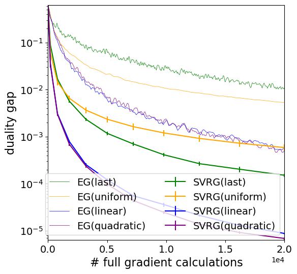
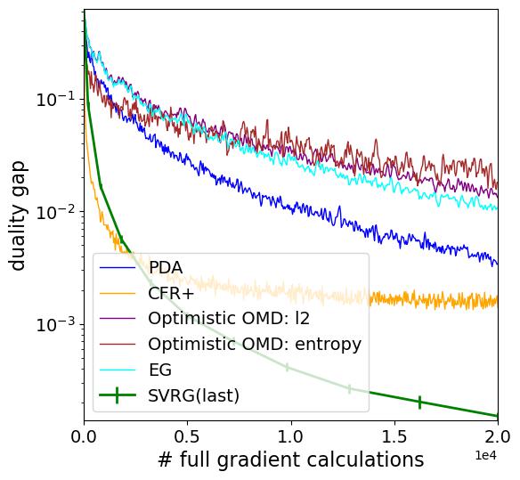
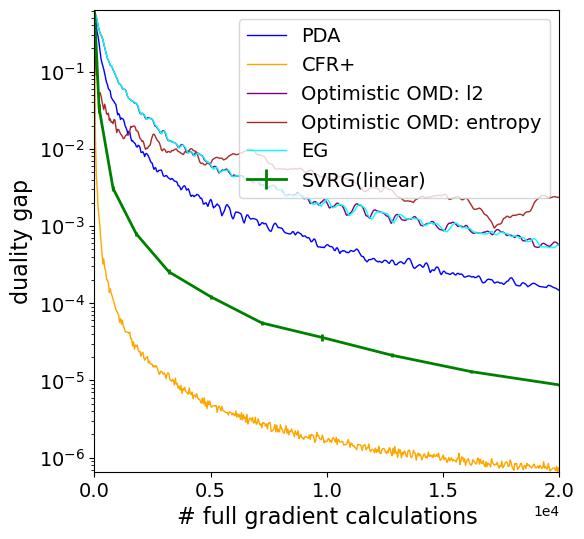
Figure 4: Numerical results on randomly generated matrix. The setup is the same as in Figure 1.

Numerical results on Nemirovski’s two symmetric matrices

We compare (loopless) SVRG-EG with EG (on the left) and other algorithms (the middle shows last-iterate and the right shows linear iterate averaging), based on Nemirovski’s two symmetric matrix classes. The results are shown in Figure 5 and Figure 6. To show fast convergence of EG-type methods, we show results of experiments in which all EG-type methods are implemented using larger stepsizes. In particular, in the first matrix game we use $20\times$ stepsizes, and in the second matrix game we use $10\times$ stepsizes. For both games, all EG-type methods still converge under the larger stepsizes. Note that even CFR+ converges fast in last iterates on some of these cases, they are not guaranteed to converge (under this stepsize).

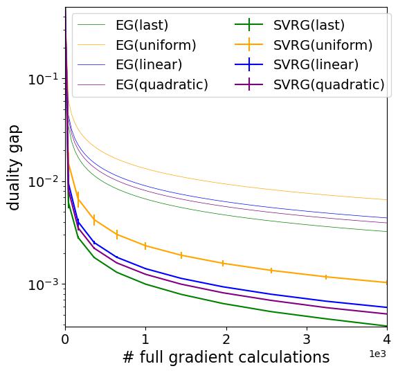
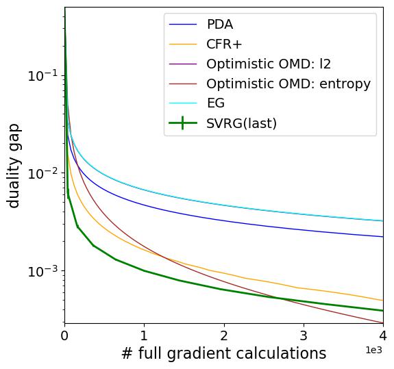
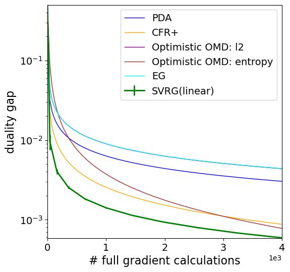
Figure 5: Numerical results on the first symmetric matrix in Nemirovski [34]. Note that Optimistic OMD (l2 norm) and EG overlap. The setup is the same as in Figure 1.

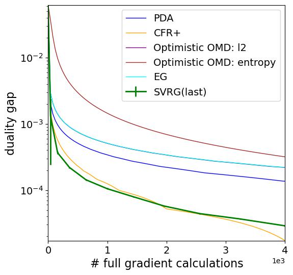
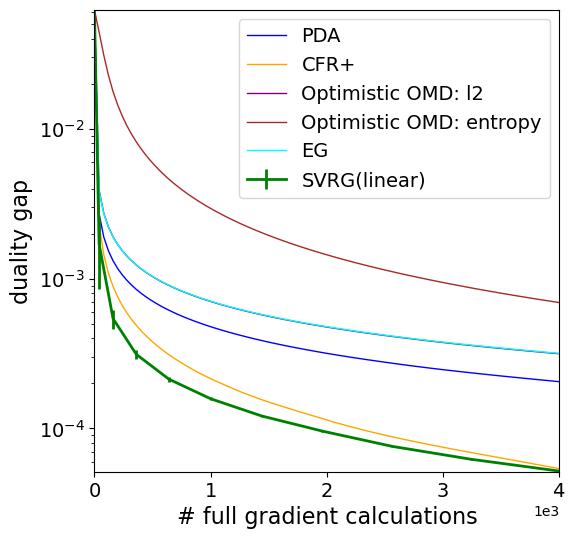
Figure 6: Numerical results on the second symmetric matrix in Nemirovski [34]. Note that Optimistic OMD (l2 norm) and EG overlap. The setup is the same as in Figure 1.

Numerical results on Leduc game

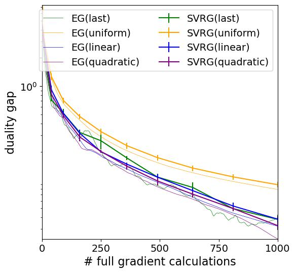
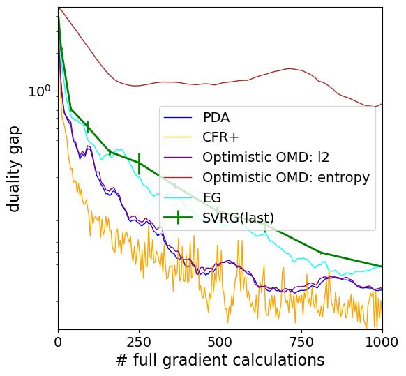
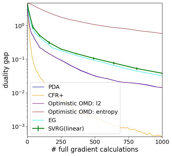
Figure 7: Numerical results on Leduc game. Random algorithms were implemented with seeds 0, 1, 2. The setup is the same as in Figure 1.

More results on image segmentation

To construct the image segmentation SPP, we use the segmentation.slic module in Scikit-image (0.19.2) package to initialize the centroids of regions using the $k$ mean method. This module segments images using k-means clustering in Color-(x,y,z) space. We show the initial image segmentation result compared to our optimized result, and additional numerical results in Figure 8.

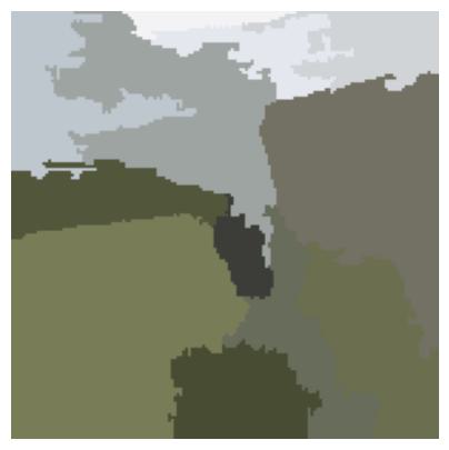
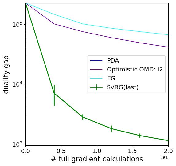
Figure 8: Left is the segmentation result from the initial $k$-means method. Middle is the segmentation result from solving Equation 12 via SVRG-EG. Random algorithms are implemented with seeds 0-5. Other setup is the same as in Figure 1. Right is numerical performance on all applicable algorithms, with last iterate. Note that PDA and Optimistic OMD overlap.

Numerical results of double-loop SVRG-EG

We implement experiments using double-loop SVRG-EG as well, and show results as follows. All setups are the same as in Figure 1, except for using double-loop version of SVRG-EG.

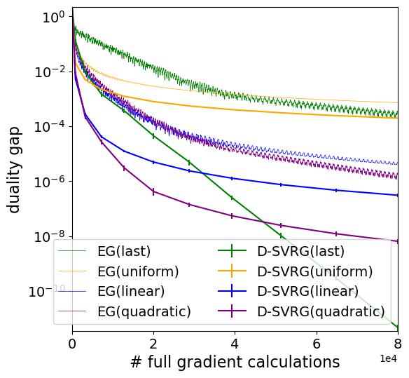
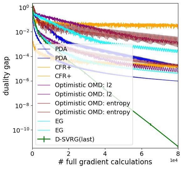
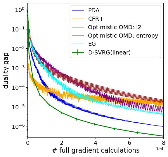
Figure 9: Numerical results on policeman and burglar game (with double-loop SVRG-EG).

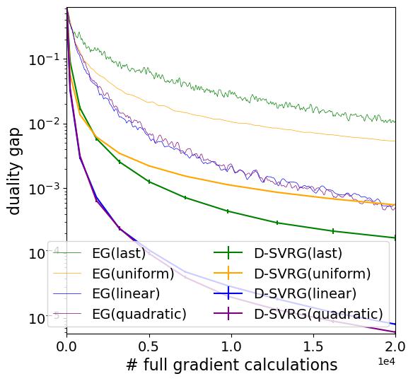
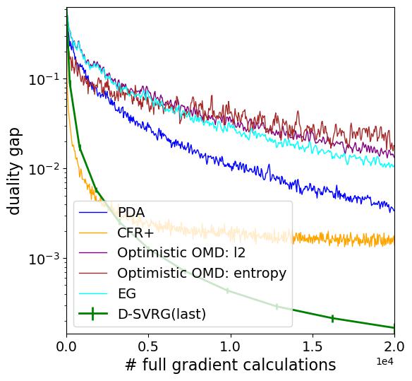
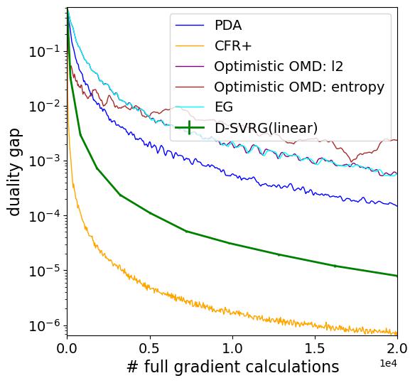
Figure 10: Numerical results on randomly generated matrix (with double-loop SVRG-EG).

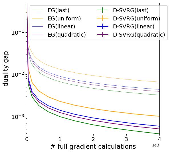
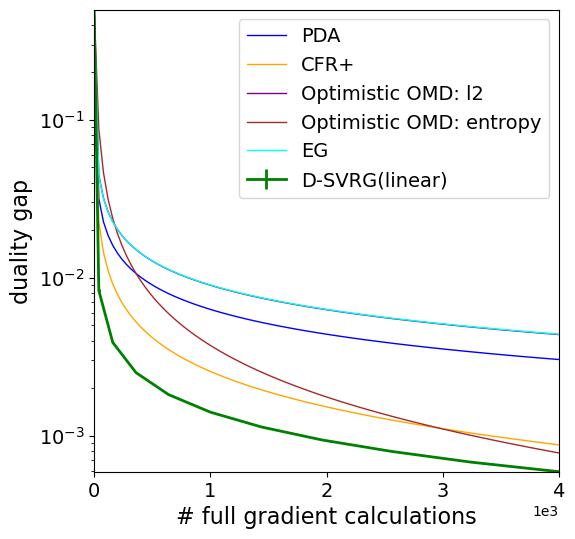
Figure 11: Numerical results on the first symmetric matrix in Nemirovski [34] (with double-loop SVRG-EG)

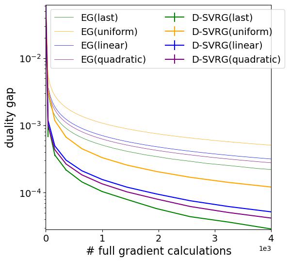
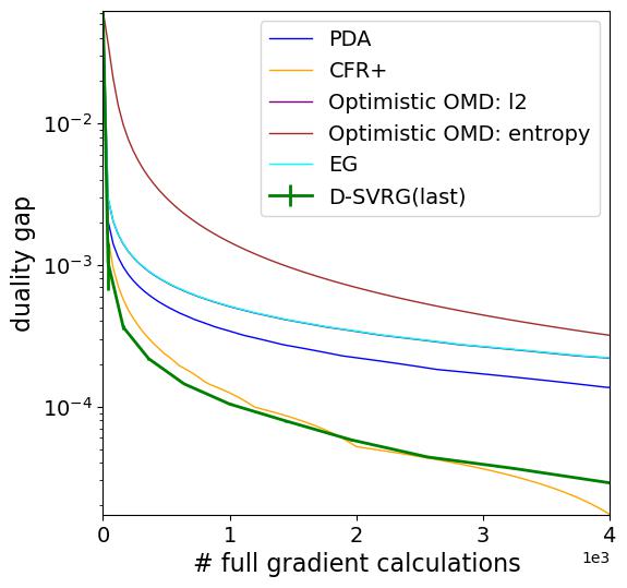
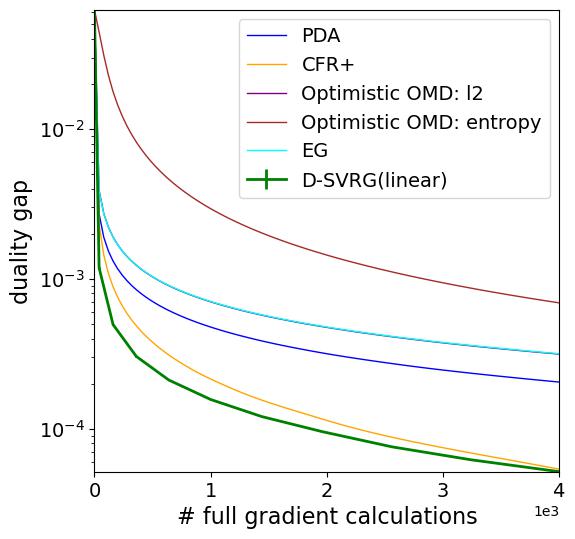
Figure 12: Numerical results on the second symmetric matrix in Nemirovski [34] (with double-loop SVRG-EG)

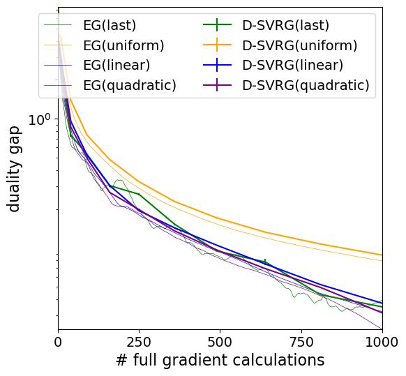
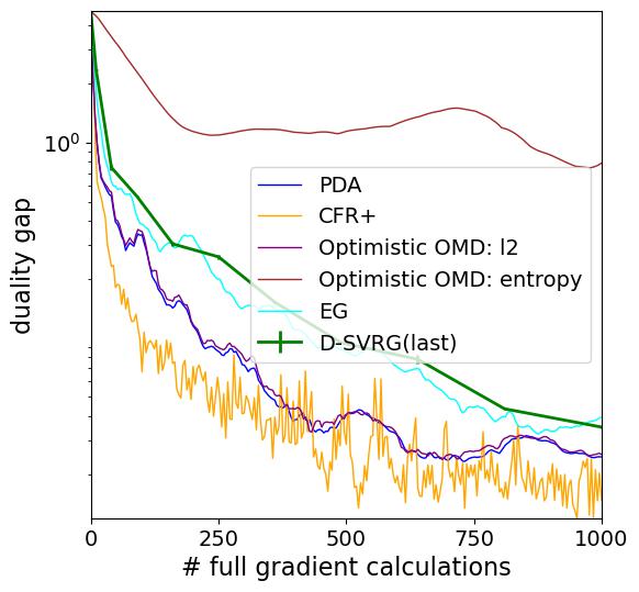
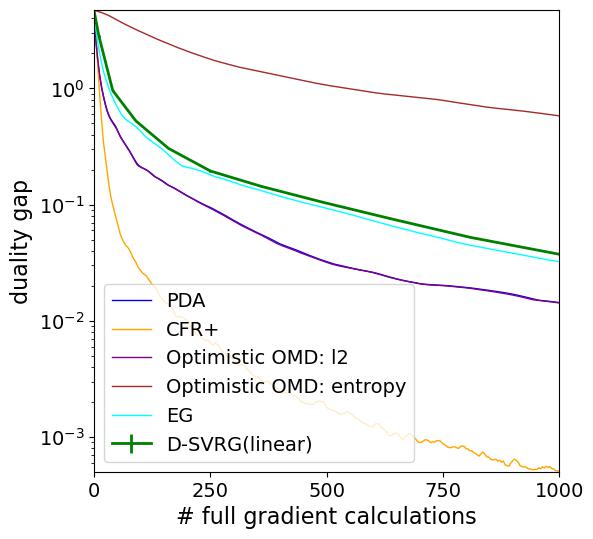
Figure 13: Numerical results on Leduc game (with double-loop SVRG-EG).

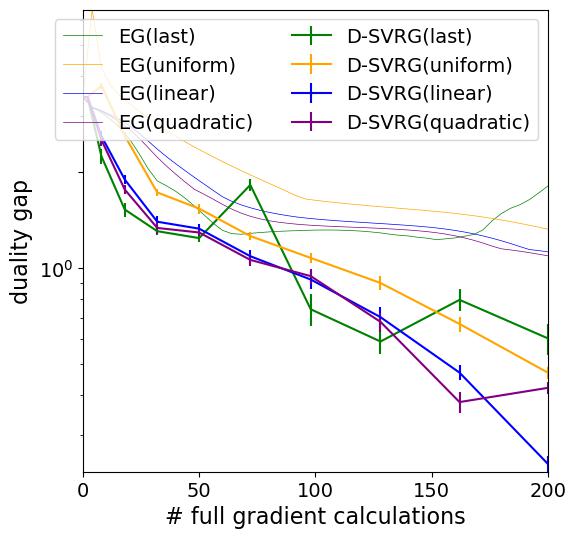
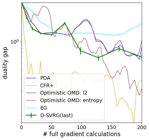
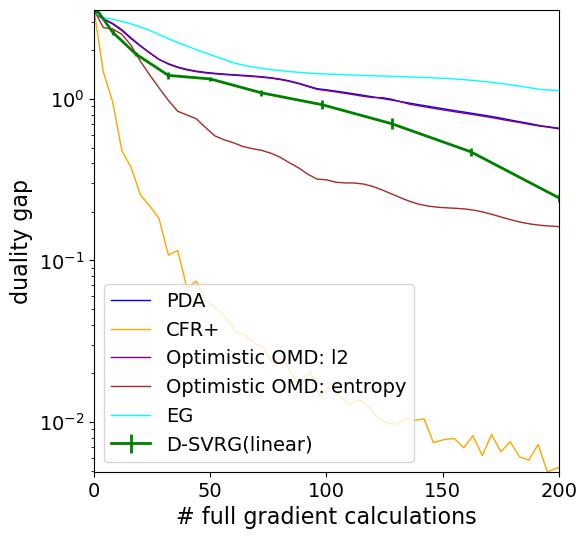
Figure 14: Numerical results on Search (zero sum) game (with double-loop SVRG-EG).

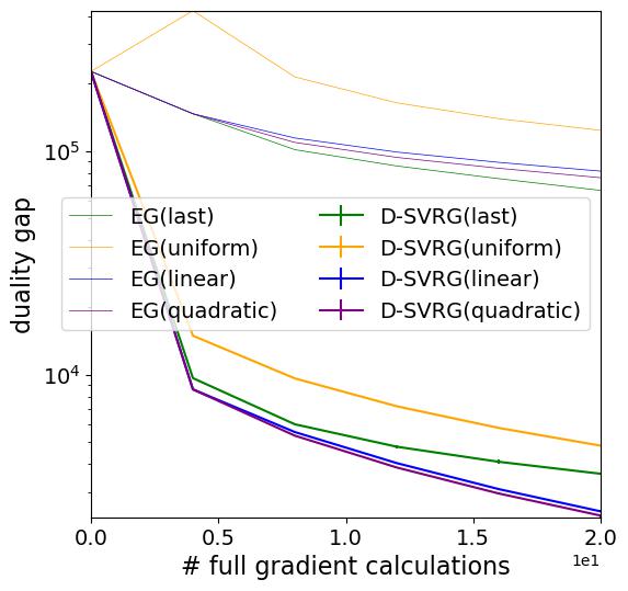
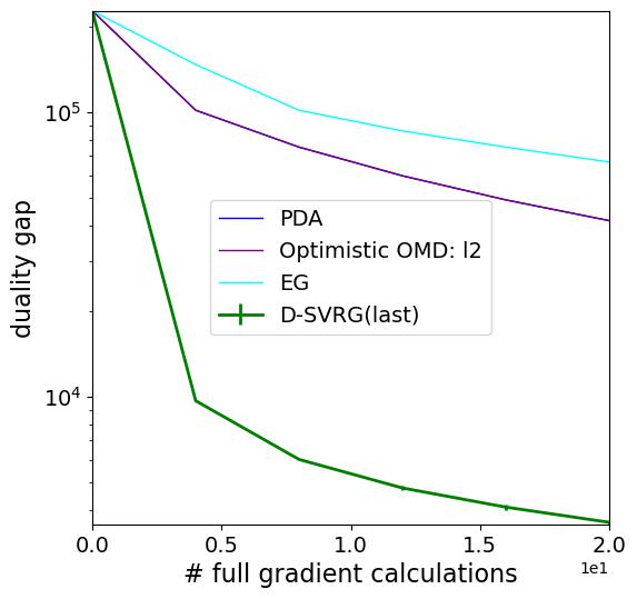
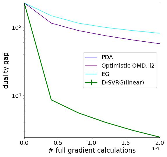
Figure 15: Numerical results on image segmentation. Left is numerical performance of double-loop SVRG-EG compared to EG. Middle and right are numerical performance on all applicable algorithms, with last iterate and linear averaging, respectively. Note that PDA and Optimistic OMD overlap.

References

- Alacaoglu and Malitsky [2022] Ahmet Alacaoglu and Yura Malitsky. Stochastic variance reduction for variational inequality methods. In Conference on Learning Theory, pages 778–816. PMLR, 2022.
- Alkousa et al. [2020] Mohammad S Alkousa, Alexander Vladimirovich Gasnikov, Darina Mikhailovna Dvinskikh, Dmitry A Kovalev, and Fedor Sergeevich Stonyakin. Accelerated methods for saddle-point problem. Computational Mathematics and Mathematical Physics, 60(11):1787–1809, 2020.
- Applegate et al. [2023] David Applegate, Oliver Hinder, Haihao Lu, and Miles Lubin. Faster first-order primal-dual methods for linear programming using restarts and sharpness. Mathematical Programming, 201(1-2):133–184, 2023.
- Beznosikov and Gasnikov [2022] Aleksandr Beznosikov and Alexander Gasnikov. Sarah-based variance-reduced algorithm for stochastic finite-sum cocoercive variational inequalities. arXiv preprint arXiv:2210.05994, 2022.
- Burke and Ferris [1993] James V Burke and Michael C Ferris. Weak sharp minima in mathematical programming. SIAM Journal on Control and Optimization, 31(5):1340–1359, 1993.
- Carmon et al. [2019] Yair Carmon, Yujia Jin, Aaron Sidford, and Kevin Tian. Variance reduction for matrix games. Advances in Neural Information Processing Systems, 32, 2019.
- Chambolle and Pock [2011] Antonin Chambolle and Thomas Pock. A first-order primal-dual algorithm for convex problems with applications to imaging. Journal of mathematical imaging and vision, 40(1):120–145, 2011.
- Chambolle and Pock [2016] Antonin Chambolle and Thomas Pock. On the ergodic convergence rates of a first-order primal–dual algorithm. Mathematical Programming, 159(1-2):253–287, 2016.
- Cheng et al. [2001] Heng-Da Cheng, X_ H_ Jiang, Ying Sun, and Jingli Wang. Color image segmentation: advances and prospects. Pattern recognition, 34(12):2259–2281, 2001.
- Defazio et al. [2014] Aaron Defazio, Francis Bach, and Simon Lacoste-Julien. Saga: A fast incremental gradient method with support for non-strongly convex composite objectives. Advances in neural information processing systems, 27, 2014.
- Deng et al. [1999] Yining Deng, B Shin Manjunath, and Hyundoo Shin. Color image segmentation. In Proceedings. 1999 IEEE Computer Society Conference on Computer Vision and Pattern Recognition (Cat. No PR00149), volume 2, pages 446–451. IEEE, 1999.
- Drusvyatskiy and Lewis [2018] Dmitriy Drusvyatskiy and Adrian S Lewis. Error bounds, quadratic growth, and linear convergence of proximal methods. Mathematics of Operations Research, 43(3):919–948, 2018.
- Du et al. [2022] Simon S Du, Gauthier Gidel, Michael I Jordan, and Chris Junchi Li. Optimal extragradient-based bilinearly-coupled saddle-point optimization. arXiv preprint arXiv:2206.08573, 2022.
- Farina et al. [2021] Gabriele Farina, Christian Kroer, and Tuomas Sandholm. Better regularization for sequential decision spaces: Fast convergence rates for nash, correlated, and team equilibria. In Proceedings of the ACM Conference on Economics and Computation, 2021.
- Gao et al. [2021] Yuan Gao, Christian Kroer, and Donald Goldfarb. Increasing iterate averaging for solving saddle-point problems. In Proceedings of the AAAI Conference on Artificial Intelligence, volume 35, pages 7537–7544, 2021.
- Han et al. [2021] Yuze Han, Guangzeng Xie, and Zhihua Zhang. Lower complexity bounds of finite-sum optimization problems: The results and construction. arXiv preprint arXiv:2103.08280, 2021.
- Hoda et al. [2010] Samid Hoda, Andrew Gilpin, Javier Pena, and Tuomas Sandholm. Smoothing techniques for computing Nash equilibria of sequential games. Mathematics of Operations Research, 35(2):494–512, 2010.
- Hsieh et al. [2019] Yu-Guan Hsieh, Franck Iutzeler, Jérôme Malick, and Panayotis Mertikopoulos. On the convergence of single-call stochastic extra-gradient methods. Advances in Neural Information Processing Systems, 32, 2019.
- Huang et al. [2022] Kevin Huang, Nuozhou Wang, and Shuzhong Zhang. An accelerated variance reduced extra-point approach to finite-sum vi and optimization. arXiv preprint arXiv:2211.03269, 2022.
- Jin et al. [2022] Yujia Jin, Aaron Sidford, and Kevin Tian. Sharper rates for separable minimax and finite sum optimization via primal-dual extragradient methods. arXiv preprint arXiv:2202.04640, 2022.
- Johnson and Zhang [2013] Rie Johnson and Tong Zhang. Accelerating stochastic gradient descent using predictive variance reduction. Advances in neural information processing systems, 26, 2013.
- Juditsky et al. [2011] Anatoli Juditsky, Arkadi Nemirovski, and Claire Tauvel. Solving variational inequalities with stochastic mirror-prox algorithm. Stochastic Systems, 1(1):17–58, 2011.
- Kannan and Shanbhag [2019] Aswin Kannan and Uday V Shanbhag. Optimal stochastic extragradient schemes for pseudomonotone stochastic variational inequality problems and their variants. Computational Optimization and Applications, 74(3):779–820, 2019.
- Karimi et al. [2016] Hamed Karimi, Julie Nutini, and Mark Schmidt. Linear convergence of gradient and proximal-gradient methods under the polyak-łojasiewicz condition. In Joint European Conference on Machine Learning and Knowledge Discovery in Databases, pages 795–811. Springer, 2016.
- Kovalev et al. [2020] Dmitry Kovalev, Samuel Horváth, and Peter Richtárik. Don’t jump through hoops and remove those loops: Svrg and katyusha are better without the outer loop. In Algorithmic Learning Theory, pages 451–467. PMLR, 2020.
- Kroer et al. [2020] Christian Kroer, Kevin Waugh, Fatma Kılınç-Karzan, and Tuomas Sandholm. Faster algorithms for extensive-form game solving via improved smoothing functions. Mathematical Programming, pages 1–33, 2020.
- Lanctot et al. [2009] Marc Lanctot, Kevin Waugh, Martin Zinkevich, and Michael Bowling. Monte carlo sampling for regret minimization in extensive games. In Advances in neural information processing systems, pages 1078–1086, 2009.
- Li et al. [2022a] Chris Junchi Li, Yaodong Yu, Nicolas Loizou, Gauthier Gidel, Yi Ma, Nicolas Le Roux, and Michael Jordan. On the convergence of stochastic extragradient for bilinear games using restarted iteration averaging. In International Conference on Artificial Intelligence and Statistics, pages 9793–9826. PMLR, 2022a.
- Li et al. [2022b] Chris Junchi Li, Angela Yuan, Gauthier Gidel, and Michael I Jordan. Nesterov meets optimism: Rate-optimal optimistic-gradient-based method for stochastic bilinearly-coupled minimax optimization. arXiv preprint arXiv:2210.17550, 2022b.
- Malitsky and Pock [2018] Yura Malitsky and Thomas Pock. A first-order primal-dual algorithm with linesearch. SIAM Journal on Optimization, 28(1):411–432, 2018.
- Malitsky and Tam [2020] Yura Malitsky and Matthew K Tam. A forward-backward splitting method for monotone inclusions without cocoercivity. SIAM Journal on Optimization, 30(2):1451–1472, 2020.
- Marcotte and Zhu [1998] Patrice Marcotte and Daoli Zhu. Weak sharp solutions of variational inequalities. SIAM Journal on Optimization, 9(1):179–189, 1998.
- Mishchenko et al. [2020] Konstantin Mishchenko, Dmitry Kovalev, Egor Shulgin, Peter Richtárik, and Yura Malitsky. Revisiting stochastic extragradient. In International Conference on Artificial Intelligence and Statistics, pages 4573–4582. PMLR, 2020.
- Nemirovski [2004] Arkadi Nemirovski. Prox-method with rate of convergence o (1/t) for variational inequalities with lipschitz continuous monotone operators and smooth convex-concave saddle point problems. SIAM Journal on Optimization, 15(1):229–251, 2004.
- Nemirovski [2013] Arkadi Nemirovski. Mini-course on convex programming algorithms, 2013.
- Nesterov [2005] Yu Nesterov. Smooth minimization of non-smooth functions. Mathematical programming, 103(1):127–152, 2005.
- Nesterov [2007] Yurii Nesterov. Dual extrapolation and its applications to solving variational inequalities and related problems. Mathematical Programming, 109(2):319–344, 2007.
- Nguyen et al. [2021] Luong V Nguyen, Qamrul Hasan Ansari, and Xiaolong Qin. Weak sharpness and finite convergence for solutions of nonsmooth variational inequalities in hilbert spaces. Applied Mathematics & Optimization, 84:807–828, 2021.
- Palaniappan and Bach [2016] Balamurugan Palaniappan and Francis Bach. Stochastic variance reduction methods for saddle-point problems. Advances in Neural Information Processing Systems, 29, 2016.
- Patriksson [1993] Michael Patriksson. A unified framework of descent algorithms for nonlinear programs and variational inequalities. Linköping University Linköping, Sweden, 1993.
- Polyak [1979] Boris Teodorovic Polyak. Sharp minima. In Proceedings of the IIASA Workshop on Generalized Lagrangians and Their Applications, Laxenburg, Austria. Institute of Control Sciences Lecture Notes, Moscow, 1979.
- Rakhlin and Sridharan [2013] Sasha Rakhlin and Karthik Sridharan. Optimization, learning, and games with predictable sequences. Advances in Neural Information Processing Systems, 26, 2013.
- Roux et al. [2012] Nicolas Roux, Mark Schmidt, and Francis Bach. A stochastic gradient method with an exponential convergence _rate for finite training sets. Advances in neural information processing systems, 25, 2012.
- Schmidt et al. [2013] Mark Schmidt, Nicolas Le Roux, and Francis Bach. Minimizing finite sums with the stochastic average gradient. arXiv e-prints, pages arXiv–1309, 2013.
- Southey et al. [2012] Finnegan Southey, Michael P Bowling, Bryce Larson, Carmelo Piccione, Neil Burch, Darse Billings, and Chris Rayner. Bayes’ bluff: Opponent modelling in poker. arXiv preprint arXiv:1207.1411, 2012.
- Syrgkanis et al. [2015] Vasilis Syrgkanis, Alekh Agarwal, Haipeng Luo, and Robert E Schapire. Fast convergence of regularized learning in games. Advances in Neural Information Processing Systems, 28, 2015.
- Tammelin [2014] Oskari Tammelin. Solving large imperfect information games using CFR+. arXiv preprint arXiv:1407.5042, 2014.
- Tseng [1995] Paul Tseng. On linear convergence of iterative methods for the variational inequality problem. Journal of Computational and Applied Mathematics, 60(1-2):237–252, 1995.
- von Stengel [1996] Bernhard von Stengel. Efficient computation of behavior strategies. Games and Economic Behavior, 14(2):220–246, 1996.
- Xu et al. [2017] Yi Xu, Qihang Lin, and Tianbao Yang. Adaptive svrg methods under error bound conditions with unknown growth parameter. Advances in Neural Information Processing Systems, 30, 2017.
- Zhang and Zhu [2022] Jin Zhang and Xide Zhu. Linear convergence of prox-svrg method for separable non-smooth convex optimization problems under bounded metric subregularity. Journal of Optimization Theory and Applications, 192(2):564–597, 2022.