Understanding Biofilm-Phage Interactions in Cystic Fibrosis Patients Using Mathematical Frameworks

Abstract

When planktonic bacteria adhere together to a surface, they begin to form biofilms, or communities of bacteria. Biofilm formation in a host can be extremely problematic if left untreated, especially since antibiotics can be ineffective in treating the bacteria. Certain lung diseases such as cystic fibrosis can cause the formation of biofilms in the lungs and can be fatal. With antibiotic-resistant bacteria, the use of phage therapy has been introduced as an alternative or an additive to the use of antibiotics in order to combat biofilm growth. Phage therapy utilizes phages, or viruses that attack bacteria, in order to penetrate and eradicate biofilms. In order to evaluate the effectiveness of phage therapy against biofilm bacteria, we adapt an ordinary differential equation model to describe the dynamics of phage-biofilm combat in the lungs. We then create our own phage-biofilm model with ordinary differential equations and stochastic modeling. Then, simulations of parameter alterations in both models are investigated to assess how they will affect the efficiency of phage therapy against bacteria. By increasing the phage mortality rate, the biofilm growth can be balanced and allow the biofilm to be more vulnerable to antibiotics. Thus, phage therapy is an effective aid in biofilm treatment.

1 Introduction

Presence of pathogenic microorganisms in our environment entail enormous problems for humans and livestock. The problem of pathogenic microrganisms is even grievous when they reside in host refr01 . Bacteria is one of such pathogenic microorganisms and they prefer to live in communities called Biofilms.

Biofilms are aggregation of bacteria on immersed surfaces and interfaces, in which the cells are embedded in a self-produced layer of extrecellular polymeric substances (EPS). The EPS gives them protection against mechanical washout and antibiotics. The formation of biofilm is often considered a virulence factor refr1 . Given the role that biofilms play in resistance, new treatments are promoted which aim at penetrating the biofilm matrix and attacking the individual cells in the biofilm. Dissolved growth-limiting substrates such as oxygen diffuse into the biofilm and undergo reaction with bacteria. In many instances, in well-developed biofilms, such growth limiting substrates might only be able to penetrate the biofilm over a relatively thin active outer layers and substantial inactive inner layers may form. Several studies has shown that there are some immaterial substances and microbes which can also penetrate the biofilm matrix, one of such microbes is the bacteriophages.

Bacteriophage, also known informally as phage, is a virus that infects and replicates within bacteria and archaea, it is among the most common disease entities in the biosphere. Bacteriophages are exclusively used as therapeutic agents to treat infections caused by pathogenic bacteria. Application of Phage therapy was dated more than a century ago with poor understanding of its potentials refr2 ; refr3 and so was overshadowed in western medicine until the emergence of bacterial strains which were resistant to antibiotics refr4 . The use of phage in treatments has a number of potential advantages over the use of antibiotics refr5 ; refr6 .

This study focuses on the interaction between biofilm and bacteriophage in phage therapy. There are two main approaches to studying phage-biofilm interactions: experimental approach, and the mathematical modeling approach. Both methods are widely utilized and each have advantages. Using mathematical models as a way to study disease dynamics is an extremely useful tool when it comes to the observation and prevention of infections in humans refr07 ; refr08 ; refr8 ; refr9 . Through the use of mathematical modeling, one is able to implement approaches in which infectious outbreaks can be predicted, assessed, and controlled refr7 ; refr8 ; refr9 . In order to model these dynamics a form of model must be chosen. These mathematical models can range from equation-based modeling, such as ordinary, partial, and stochastic differential equations, to agent-based modeling refr10 ; refr11 . From different studies that utilized mathematical modeling, findings have been made on in-host disease dynamics. Through the use of differential equations in a study conducted by Beke et. al., the disease dynamics in a bacteria-phage interaction are examined. The results of this study gathered that disease dynamics can be contingent on environmental factors such as a change in pH or temperature refr12 . In a separate study conducted by Bardina et. al., a different approach involving a stochastic model is used in order to analyze these dynamics. Upon these findings, there existed equilibria such that pathogens could be eliminated from the host or could persist depending on the levels of noise within the environment refr13 . Similarly, through differential equations and Monte Carlo simulations, Sinha et. al. evaluate which mathematical model is adequate for modeling the dynamics between phage and bacteria. In this study, it was found that disease dynamics can differ if there are spatial restrictions introduced to the model and the type of model used to describe such dynamics should reflect this restriction refr14 . These mathematical models are not only used for examining in-host dynamics, but are also used to address various phenomena. Some of these phenomena include spatial phenomena as previously mentioned, evolutionary game theory, and dynamic optimization.

Mathematical models for bacterial biofilm over the years have greatly helped in the understanding of biofilm processes such as biofilm formation and growth; detachment and its inducers refr15 ; refr015 ; refr16 ; refr17 ; refr18 . Many of the experimental and modeling studies of biofilm-phage interactions and interplay has focused on biofilm formed on surfaces other than in-host, mathematical modeling that focus on the biofilm-phage interactions and interplay in immunocompromised patents is still in its infancy. There are several immunocompromised patents that suffer from biofilm infection, we will be considering the case of biofilm formation in the lungs of Cystic Fibrosis patients.

Over the last two decades, a large number of models have been produced in order to represent the interactions between bacteria, biofilm, and bacteriophages. Some of these models involve ODEs, PDEs, agent based modeling, or stochastic models, but all of which attempt to recreate results that could be produced in an experiment in order to better and more quickly understand and predict these interactions. In a recent review from Sinha, et. al., we find models utilizing PDE’s, ODE’s, stochastic differential equations and Monte Carlo simulations. This review compares models subject to spatial constraints with those without spatial constraints refr14 .

In this study, the objective is to develop a mathematical framework to understand the different factors that contribute most during bacterial-phage interactions in biofilm setting and planktonic phage.

2 Methods

2.1 Basic model assumptions

We develop a mathematical model that describes the dynamics of biofilm-phage interactions in matured biofilms. There are two specific regions involved in this system, namely: the Biofilm region, this is the region where the bacterial cells are accumulated and formed biofilm; and the Planktonic region, this is the flow region of the bronchiole comprising of air and fluid (see Figure 1). We assume that (a) both bacteria and phages can be converted from one region to the other (b) conversion of biofilm bacteria to planktonic bacteria is induced by phages (c) phages conversion rate between biofilm and the planktonic phase is assumed to be constant, and (d) the conversion of phages from one region to the other does not change their characteristics.

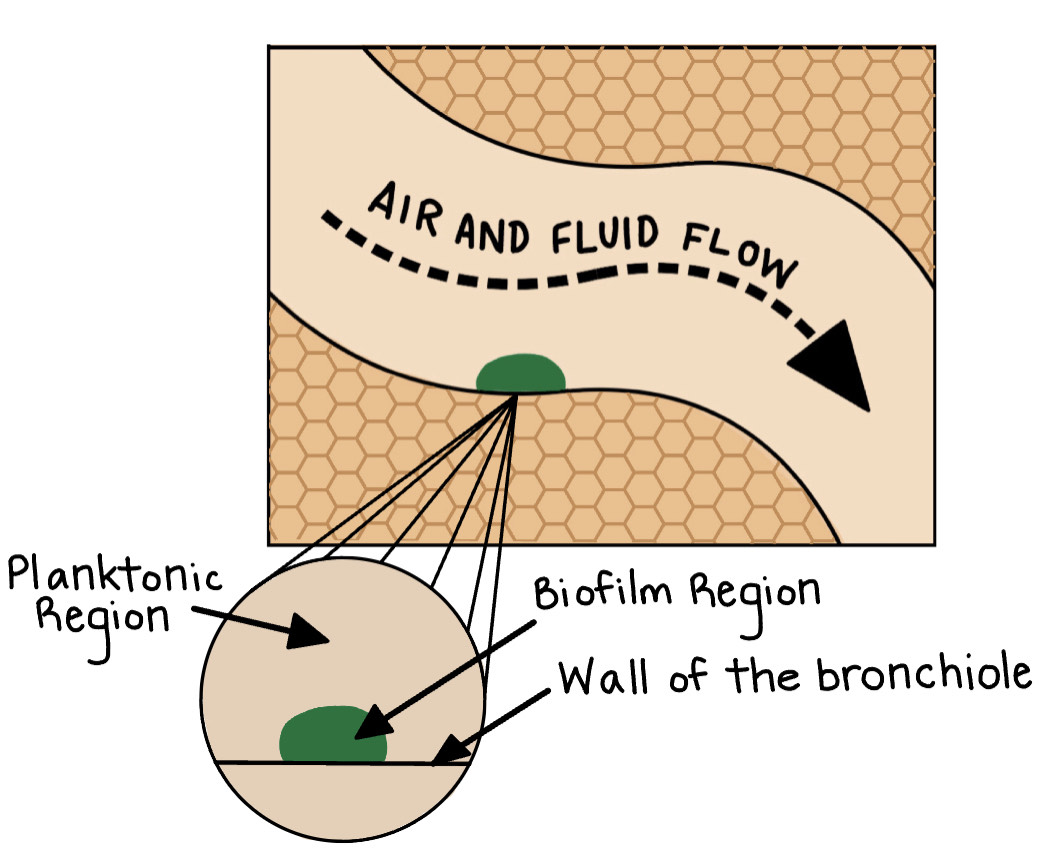
Figure 1: Schematic of Biofilm in Bronchiole This is a schematic representation of the biofilm that formed on the wall of the bronchiole, showing the biofilm region and the planktonic region

2.2 Deterministic Model - ODE

The model describing the Biofilm-Phage interactions is formulated as a deterministic model of as system of six ordinary differential equations. The dependent variables are $n$, $B$, $P$, $V_{B}$, $V_{P}$ and $I$. The variable $n$ denotes the concentration of the bacteria growth limiting nutrient substrate, $B$ denotes the bacteria cells in the biofilm region while $P$ denotes the bacterial cells in the planktonic region, $V_{B}$ and $V_{P}$ denotes the viral load of bacteriophages in the biofilm and the planktonic regions respectively; $I$ is the concentration of all the infected bacteria cells from the planktonic and biofilm regions. The model captures the detachment of bacteria cells from the biofilm induced by bacteriophages, and reattachment of bacteria to the biofilm, this meshes well with the life cycle of biofilms. The governing equations read

$$\frac{\mathrm{d}}{\mathrm{d}t}n = f(n)-\left(\lambda_{B}B+\lambda_{P}P\right)\frac{n}{n+k}$$ (1)

$$\frac{\mathrm{d}}{\mathrm{d}t}B = \lambda_{B}B\frac{n}{n+k}-\phi_{1}BV_{B}-\gamma_{1}\frac{V_{B}}{\zeta_{1}+V_{B}}B+\gamma_{2}\frac{B}{\zeta_{2}+B}P-\mu_{B}B$$ (2)

$$\frac{\mathrm{d}}{\mathrm{d}t}P = \lambda_{P}P\frac{n}{n+k}-\phi_{2}PV_{P}+\gamma_{1}\frac{V_{B}}{\zeta_{1}+V_{B}}B-\gamma_{2}\frac{B}{\zeta_{2}+B}P-\mu_{P}P$$ (3)

$$\frac{\mathrm{d}}{\mathrm{d}t}V_{B} = \beta\phi_{1}V_{B}B-c_{1}V_{B}-qV_{B}+pV_{P}$$ (4)

$$\frac{\mathrm{d}}{\mathrm{d}t}V_{P} = \beta\phi_{2}V_{P}P-c_{2}V_{P}+qV_{B}-pV_{P}$$ (5)

$$\frac{\mathrm{d}}{\mathrm{d}t}I = \phi_{1}V_{B}B+\phi_{2}V_{P}P-\frac{10}{\tau}\frac{n}{n+k}I-\alpha I$$ (6)

Figure 2: Flow diagram of the deterministic ODE model This is a schematic representation of the deterministic ODE model, showing the flows and connections with the parameters. These parameters are also presented in Table 1 with the actual descriptions of the parameter, the values and sources. Because of lack of better word, we have used ‘migration’ to capture the conversion from biofilm to planktonic region, this does not imply any spatial component.

Equation (2) and (3) describe the bacterial growth in the planktonic and biofilm regions, the equations also describe predation of bacteria by the phages and biofilm cell detachment which forms a direct coupling of the system. Equations (4) and (5) describes the phage growth in the biofilm and planktonic region, while equation (6) keeps track of all infected bacterial cells in both the biofilm and planktonic regions. Equation (1) describes the consumption of nutrient by $B$ and $P$ respectively. The flow diagram of the model is presented in Figure 2. The parameters on this model are presented in Table 1, one of the parameter of interest is the burst size which determines the average number of phage release per bacterium; and could vary from $10$ to $100$ for DNA transducing bacteriophages to about $20,000$ pfu for the RNA viruses.

Table 1: Table of parameters

Table of Parameters
Symbol	Description	Value	Units	Source
$n_{0}$	Initial Nutrient concentration	variable	$[gm^{-3}]$	refr19 ; refr15
$B_{0}$	Initial biofilm bacteria	variable	$[gm^{-3}]$	refr19 ; refr15
$P_{0}$	Initial planktonic bacteria	variable	$[gm^{-3}]$	refr19
$V_{b0}$	Initial biofilm phages	variable	$[gm^{-3}]$	Assumed
$V_{p0}$	Initial planktonic phages	variable	$[gm^{-3}]$	refr19
$I_{0}$	Initial Infected cells	variable	$[gm^{-3}]$	refr19
$p$	Phage detachement rate	$0.1$	$[d^{-1}]$	Assumed
$q$	Phage reattach rate	$0.5$	$[d^{-1}]$	Assumed
$\lambda_{B}$	biofilm bacteria growth rate	$6.0$	$[d^{-1}]$	refr19
$\lambda_{P}$	Planktonic bacteria growth rate	$6.0$	$[d^{-1}]$	refr19
$\tau$	Average latency time	$0.5$	$[h]$	refr19 ; refr20
$k$	Monod constant	$4.0$	$[gm^{-3}]$	refr19
$\alpha$	Infection decay rate	$0.2$	$[d^{-1}]$	Assumed
$\beta$	Burst size	$100$	$[-]$	refr19
$\gamma_{1}$	Phage induced detach rate	$0.6$	$[d^{-1}]$	refr15
$\gamma_{2}$	Natural detach rate	$0.3$	$[d^{-1}]$	refr15
$\phi_{1}$	Predation rate in biofilm	$10^{-8}$	$[m^{3}g^{-1}d^{-1}]$	Assumed
$\phi_{2}$	Predation rate in planktonic	$10^{-6}$	$[m^{3}g^{-1}d^{-1}]$	Assumed
$\zeta_{1}$	Monod saturation	$10^{2}$	$[gm^{-3}]$	Assumed
$\zeta_{2}$	Monod saturation	$10^{4}$	$[gm^{-3}]$	Assumed
$c_{1}$	Phage mortality rate in biofilm	$2.1$	$[d^{-1}]$	Assumed
$c_{2}$	Phage mortality rate in planktonic	$2.1$	$[d^{-1}]$	Assumed
$\mu_{B}$	Bacteria mortality rate in Biofilm	$0.1$	$[d^{-1}]$	Assumed
$\mu_{P}$	Bacteria mortality rate in planktonic	$0.1$	$[d^{-1}]$	Assumed

2.2.1 Basic Reproduction Number

The system (1)-(6) represents a nonlinear system of ODEs with the interaction of phages and bacteria.

Remark 1.

The function $f(n)$, for the input/increase of nutrients, holds that

1. $f(0)=0$ (thus making the origin an steady state) and $f^{\prime}(0)>0$.

2. For some fixed value $x>0$, the conditions $f(x)=0$ and $f^{\prime}(x)<0$ are held.

Considering the above properties, we compute the Jacobian matrix which is given by:

$$J(X,\mathcal{P})=\left(\scalebox{0.65}{\mbox{$\displaystyle\begin{array}[]{cccccc}f^{\prime}(n)-\frac{k(\lambda_{B}B+\lambda_{P}P)}{(n+k)^{2}}&-\frac{n\lambda_{B}}{n+k}&-\frac{n\lambda_{P}}{n+k}&0&0&0\\ \frac{kB\lambda_{B}}{(n+k)^{2}}&{\dagger}&\frac{B\gamma_{2}}{\zeta_{2}+B}&-\phi_{1}B-\frac{\zeta_{1}\gamma_{1}B}{(\zeta_{1}+V_{B})^{2}}&0&0\\ \frac{\lambda_{P}Pk}{(n+k)^{2}}&\frac{\gamma_{1}V_{B}}{\zeta_{1}+V_{B}}-\frac{\gamma_{2}\zeta_{2}P}{(\zeta_{2}+B)^{2}}&{\ddagger}&\frac{\gamma_{1}\zeta_{1}B}{(\zeta_{1}+V_{B})^{2}}&-\phi_{2}P&0\\ 0&\beta\phi_{1}V_{B}&0&\beta\phi_{1}B-c_{1}-q&p&0\\ 0&0&\beta\phi_{2}V_{P}&q&\beta\phi_{2}P-p-c_{2}&0\\ -\frac{10kI}{\tau(n+k)^{2}}&\phi_{1}V_{B}&\phi_{2}V_{P}&\phi_{1}B&\phi_{2}P&-\frac{10n}{\tau(n+k)}-\alpha\end{array}$}}\right)$$ (7)

where

$$\begin{split}{\dagger}&=\frac{n\lambda_{B}}{n+k}-\phi_{1}V_{B}-\frac{\gamma_{1}V_{B}}{\zeta_{1}+V_{B}}+\frac{\gamma_{2}\zeta_{2}P}{(\zeta_{2}+B)^{2}}-\mu_{B}\\ {\ddagger}&=\frac{\lambda_{P}n}{n+k}-\phi_{2}V_{P}-\frac{\gamma_{2}B}{\zeta_{2}+B}-\mu_{P}\end{split}$$

The equilibria points are determined by the zeros of the system (1)-(6). Considering the disease free equilibria which are mainly determined in the absence of pathogen scenario, that is, when neither phages and infected bacterial cells are present. From this context, we let $I=0$, $V_{P}=0$, and $V_{B}=0$; notice this condition causes for (4),(5), and (6) to equal zero, thus reducing the equilibria problem to find the zeros of the system

$$\begin{split}\frac{\mathrm{d}}{\mathrm{d}t}n&=f(n)-\left(\lambda_{B}B+\lambda_{P}P\right)\frac{n}{n+k}\\ \frac{\mathrm{d}}{\mathrm{d}t}B&=B\left(\frac{\lambda_{B}n}{n+k}+\frac{\gamma_{2}P}{\zeta_{2}+B}-\mu_{B}\right)\\ \frac{\mathrm{d}}{\mathrm{d}t}P&=P\left(\frac{\lambda_{P}n}{n+k}-\frac{\gamma_{2}B}{\zeta_{2}+B}-\mu_{P}\right)\end{split}$$ (8)

Through a quick inspection we have that the equilibria points of (8) are

$$DFE_{1} = \left(\scalebox{1.0}{\mbox{$\displaystyle n,0,0,0,0,0$}}\right)\mathchar 24635\relax\;\qquad\qquad\mbox{where $n$ is a zero of the function $f$}$$

$$DFE_{2} = \left(\scalebox{0.85}{\mbox{$\displaystyle\frac{k\mu_{B}}{\lambda_{B}-\mu_{B}},\frac{f\left(\frac{k\mu_{B}}{\lambda_{B}-\mu_{B}}\right)\left(\frac{k\mu_{B}}{\lambda_{B}-\mu_{B}}+k\right)}{\lambda_{B}\frac{k\mu_{B}}{\lambda_{B}-\mu_{B}}},0,0,0,0$}}\right)=\left(n_{B}^{\ast},\frac{f(n_{B}^{\ast})}{\mu_{B}},0,0,0,0\right)$$

$$DFE_{3} = \left(\scalebox{0.75}{\mbox{$\displaystyle\frac{k\mu_{P}}{\lambda_{P}-\mu_{P}},0,\frac{f\left(\frac{k\mu_{P}}{\lambda_{P}-\mu_{P}}\right)\left(\frac{k\mu_{P}}{\lambda_{P}-\mu_{P}}+k\right)}{\lambda_{P}\frac{k\mu_{P}}{\lambda_{P}-\mu_{P}}},0,0,0$}}\right)=\left(n_{P}^{\ast},0,\frac{f(n_{P}^{\ast})}{\mu_{P}},0,0,0\right)$$

By evaluating (7) at (2.2.1) we have that

$$J_{0,1}=\left(\begin{array}[]{cccccc}f^{\prime}(n)&-\frac{\lambda_{B}n}{n+k}&-\frac{\lambda_{P}n}{n+k}&0&0&0\\ 0&\frac{\lambda_{B}n}{n+k}-\mu_{B}&0&0&0&0\\ 0&0&\frac{\lambda_{P}n}{n+k}-\mu_{P}&0&0&0\\ 0&0&0&-c_{1}-q&p&0\\ 0&0&0&q&-c_{2}-p&0\\ 0&0&0&0&0&-\frac{10n}{\tau(n+k)}-\alpha\end{array}\right)$$ (9)

which can be rewritten as the difference of two positive matrices $\mathcal{F}_{1}$ and $\mathcal{V}_{1}$, thus we apply the next generation matrix. The basic reproductive number is therefore given by the spectral radius of $\mathcal{F}_{1}\mathcal{V}_{1}^{-1}$, which is the eigenvalue of largest magnitude, thus

$$R_{0,1}=\max\left\{\frac{\lambda_{B}n}{\mu_{B}(n+k)},\frac{\lambda_{P}n}{\mu_{P}(n+k)},\pm\sqrt{\frac{pq}{(c_{1}+q)(c_{2}+p)}}\right\}$$ (10)

Theorem 1.

The Disease-Free equilibrium 1 (DFE1) is asymptotically stable if $n\neq 0$ and $R_{0,1}<1$

Proof:

Suppose $n=0$, a zero of $f$, considering Remark 1, in this case the system naturally becomes unstable since (9) has positive eigenvalues, so it suffices that $n>0$ be a zero of $f$.

Remains to show $R_{0,1}<1$ for stability: For this, the overall stability of $DFE1=(n,0,0,0,0,0)$ is given by the roots of the characteristic polynomial of (9) which is

$det(\lambda I-J_{0,1})=$

$det\left(\begin{array}[]{cccccc}\lambda-f^{\prime}(n)&\frac{\lambda_{B}n}{n+k}&\frac{\lambda_{P}n}{n+k}&0&0&0\\ 0&\lambda+\mu_{B}-\frac{\lambda_{B}n}{n+k}&0&0&0&0\\ 0&0&\lambda-\frac{\lambda_{P}n}{n+k}+\mu_{P}&0&0&0\\ 0&0&0&\lambda+c_{1}+q&-p&0\\ 0&0&0&-q&\lambda+c_{2}+p&0\\ 0&0&0&0&0&\lambda+\frac{10n}{\tau(n+k)}+\alpha\end{array}\right)=$

$(\lambda-f^{\prime}(n))\left(\lambda+\mu_{B}-\frac{\lambda_{B}n}{n+k}\right)\left(\lambda-\frac{\lambda_{P}n}{n+k}+\mu_{P}\right)\left(\lambda+\frac{10n}{\tau(n+k)}+\alpha\right)\left(\left[\lambda+c_{1}+q\right]\left[\lambda+c_{2}+p\right]-pq\right)$

whose roots are all negative if the following holds:

$$\mu_{B}>\frac{\lambda_{B}n}{n+k}\,,\quad\frac{\lambda_{P}n}{n+k}<\mu_{P}\,,\quad\left[\lambda+c_{1}+q\right]\left[\lambda+c_{2}+p\right]<pq$$

Notice that when $R_{0,1}<1$, the conditions above hold. Hence $DFE1$ is asymptotically stable.

Similarly, for the second disease free equilibrium (DFE2) we have that

$J_{0,2}=\left(\begin{array}[]{cccccc}f^{\prime}(n_{B}^{\ast})-k^{\star}&-q^{\star}\lambda_{B}&-q^{\star}\lambda_{P}&0&0&0\\ k^{\star}&q^{\star}\lambda_{B}-\mu_{B}&s^{\star}&-t^{\star}\phi_{1}-\frac{\gamma_{1}t^{\star}}{\zeta_{1}}&0&0\\ 0&0&q^{\star}\lambda_{P}-s^{\star}\mu_{P}&\frac{\gamma_{1}t^{\star}}{\zeta_{1}}&0&0\\ 0&0&0&\beta t^{\star}\phi_{1}-c_{1}-q&p&0\\ 0&0&0&q&-p-c_{2}&0\\ 0&0&0&t^{\star}\phi_{1}&0&-\frac{10q^{\star}}{\tau}-\alpha\end{array}\right)$

$k^{\star}=\frac{k\lambda_{B}f(n_{B}^{\ast})}{\mu_{B}(n_{B}^{\ast}+k)^{2}}$, $q^{\star}=\frac{n_{B}^{\ast}}{n_{B}^{\ast}+k}$, $s^{\star}=\frac{f(n_{B}^{\ast})\gamma_{2}}{\mu_{B}\zeta_{2}+f(n_{B}^{\ast})}$, $t^{\star}=\frac{f(n_{B}^{\ast})}{\mu_{B}}$

which can be rewritten as the difference of two positive matrices $\mathcal{F}_{1}$ and $\mathcal{V}_{1}$, thus we apply the next generation matrix. The basic reproductive number is therefore given by the spectral radius of $\mathcal{F}_{1}\mathcal{V}_{1}^{-1}$ which is the eigenvalue of largest magnitude, thus

$$R_{0,2}=\max\left\{\frac{k\lambda_{B}f(n_{B}^{*})}{\lvert f^{\prime}(n_{B}^{*})\rvert\mu_{B}(n_{B}^{*}+k)^{2}+k\lambda_{B}f(n_{B}^{*})},\frac{(\mu_{B}\xi_{2}+f(n_{B}^{*}))\lambda_{P}\eta_{B}^{*}}{(n_{B}^{*}+k)\{\gamma_{2}f(n_{B}^{*})+\mu_{P}(\mu_{B}\xi_{2}+f(n_{B}^{*}))\}},\frac{\phi_{1}f(n_{B}^{*})}{\mu_{B}(c_{1}+q)}\right\}$$ (11)

Theorem 2.

The Disease-Free equilibrium 2 (DFE2) is asymptotically stable if $n_{B}^{\ast}\neq 0$, $f^{\prime}(n_{B}^{\ast})\gg 0$ and $R_{0,2}<1$

Proof: Suppose $n=0$, a zero of $f$, considering Remark 1, in this case the system naturally becomes unstable since the DFE2 Jacobian matrix has positive eigenvalues, so it suffices that $n>0$ be a zero of $f$.

Remains to show $R_{0,2}<1$ for stability: For this, the overall stability of $DFE2=\left(n_{B}^{\ast},\frac{f(n_{B}^{\ast})}{\mu_{B}},0,0,0,0\right)$ is given by the roots of the characteristic polynomial of DFE2 Jacobian matrix which is

$det(\lambda I-J_{0,2})=$

$det\left(\begin{array}[]{cccccc}\lambda-f^{\prime}(n_{B}^{\ast})+k^{\star}&q^{\star}\lambda_{B}&q^{\star}\lambda_{P}&0&0&0\\ -k^{\star}&\lambda-q^{\star}\lambda_{B}+\mu_{B}&-s^{\star}&t^{\star}\phi_{1}+\frac{\gamma_{1}t^{\star}}{\zeta_{1}}&0&0\\ 0&0&\lambda-q^{\star}\lambda_{P}+s^{\star}\mu_{P}&\frac{\gamma_{1}t^{\star}}{\zeta_{1}}&0&0\\ 0&0&0&\lambda-\beta t^{\star}\phi_{1}+c_{1}+q&p&0\\ 0&0&0&q&\lambda+p+c_{2}&0\\ 0&0&0&-t^{\star}\phi_{1}&0&\lambda+\frac{10q^{\star}}{\tau}+\alpha\end{array}\right)$

where,

$k^{\star}=\frac{k\lambda_{B}f(n_{B}^{\ast})}{\mu_{B}(n_{B}^{\ast}+k)^{2}}$, $q^{\star}=\frac{n_{B}^{\ast}}{n_{B}^{\ast}+k}$, $s^{\star}=\frac{f(n_{B}^{\ast})\gamma_{2}}{\mu_{B}\zeta_{2}+f(n_{B}^{\ast})}$, $t^{\star}=\frac{f(n_{B}^{\ast})}{\mu_{B}}$

whose roots are all negative if the following holds:

• If $f^{\prime}(n_{B}^{\ast})+\frac{n_{B}^{\ast}\lambda_{B}}{n_{B}^{\ast}+k}<\frac{k\lambda_{B}f(n_{B}^{\ast})}{\mu_{B}(n_{B}^{\ast}+k)^{2}}+\mu_{B}$,

  • since phages are gone, and bacteria is growing, we expect the mortality rate of bacteria to be negligible when compared with the growth rate.

• $f^{\prime}(n_{B}^{\ast})+\frac{n_{B}^{\ast}\lambda_{B}}{n_{B}^{\ast}+k}<\frac{k\lambda_{B}f(n_{B}^{\ast})}{\mu_{B}(n_{B}^{\ast}+k)^{2}}+\mu_{B}$

  • this means that the bacteria growth in the biofilm is greater than the bacteria death, this sounds right since DFE of phages in the biofilm implies loosing more phages and having more bacteria

• $(c_{2}+p)c_{1}+qc_{2}>\frac{\beta\phi_{1}f(n_{B}^{\ast})(c_{2}+p)}{\mu_{P}}$

  • this means that the phage loss in the biofilm is greater than phage growth

Notice that when $R_{0,2}<1$, the conditions above hold. Hence $DFE2$ is asymptotically stable. This concludes the proof. Finally, for the third disease free equilibrium (DFE3) we have that

$J_{0,3}=$

$$\left(\begin{array}[]{cccccc}f^{\prime}(n_{P}^{\ast})-\frac{k\lambda_{P}f(n_{P}^{\ast})}{\mu_{P}(n_{P}^{\ast}+k)^{2}}&-\frac{n_{P}^{\ast}\lambda_{B}}{n_{P}^{\ast}+k}&-\frac{n_{P}^{\ast}\lambda_{P}}{n_{P}^{\ast}+k}&0&0&0\\ 0&\frac{n_{P}^{\ast}\lambda_{B}}{n_{P}^{\ast}+k}+\frac{\gamma_{2}f(n_{P}^{\ast})}{\mu_{P}\zeta_{2}}-\mu_{B}&0&0&0&0\\ \frac{\lambda_{P}kf(n_{P}^{\ast})}{\mu_{P}(n_{P}^{\ast}+k)^{2}}&-\frac{\gamma_{2}f(n_{P}^{\ast})}{\mu_{P}\zeta_{2}}&\frac{\lambda_{P}n_{P}^{\ast}}{n_{P}^{\ast}+k}-\mu_{P}&0&-\phi_{2}\frac{f(n_{P}^{\ast})}{\mu_{P}}&0\\ 0&0&0&-c_{1}-q&p&0\\ 0&0&0&q&\beta\phi_{2}\frac{f(n_{P}^{\ast})}{\mu_{P}}-p-c_{2}&0\\ 0&0&0&0&\phi_{2}\frac{f(n_{P}^{\ast})}{\mu_{P}}&-\frac{10n_{P}^{\ast}}{\tau(n_{P}^{\ast}+k)}-\alpha\end{array}\right)$$

which can be rewritten as the difference of two positive matrices $\mathcal{F}_{1}$ and $\mathcal{V}_{1}$, thus we apply the next generation matrix. The basic reproductive number is therefore given by the spectral radius of $\mathcal{F}_{1}\mathcal{V}_{1}^{-1}$ which is the eigenvalue of largest magnitude, thus

$$\begin{split}R_{0,3}=\max\left\{\frac{n_{P}^{\ast}\lambda_{B}}{\mu_{B}(n_{P}^{\ast}+k)}+\frac{\gamma_{2}f(n_{P}^{\ast})}{\mu_{P}\mu_{B}\zeta_{2}},\right.&\left.\frac{\lambda_{P}n_{P}^{\ast}}{\mu_{P}(n_{P}^{\ast}+k)}\left[1-\frac{k\lambda_{P}f(n_{P}^{\ast})}{\lvert f^{\prime}(n_{P}^{\ast})\rvert\mu_{P}(n_{P}^{\ast}+k)^{2}+k\lambda_{P}f(n_{P}^{\ast})}\right],\right.\\ &\qquad\left.\frac{\beta\phi_{2}f(n_{P}^{\ast})}{2\mu_{P}(c_{2}+p)}\pm\sqrt{\left(\frac{\beta\phi_{2}f(n_{P}^{\ast})}{2\mu_{P}(c_{2}+p)}\right)^{2}+\frac{pq}{(c_{1}+q)(c_{2}+p)}}\right\}\end{split}$$ (12)

Theorem 3.

The Disease-Free equilibrium 3 (DFE3) is asymptotically stable if $n\neq 0$, $f^{\prime}(n)\gg 0$ and $R_{0,3}<1$

Proof: Suppose $n=0$, a zero of $f$, considering Remark 1, in this case the system naturally becomes unstable since the DFE3 Jacobian matrix has positive eigenvalues, so it suffices that $n>0$ be a zero of $f$.

Remains to show $R_{0,3}<1$ for stability: For this, the overall stability of $DFE3=\left(n_{P}^{\ast},0,\frac{f(n_{P}^{\ast})}{\mu_{P}},0,0,0\right)$ is given by the roots of the characteristic polynomial of DFE3 Jacobian matrix which is

$$\begin{split}det(\lambda I-J_{0,3})=&\left\lvert\begin{array}[]{ccc}\lambda-f^{\prime}(n_{P}^{\ast})+\frac{k\lambda_{P}f(n_{P}^{\ast})}{\mu_{P}(n_{P}^{\ast}+k)^{2}}&\frac{n_{P}^{\ast}\lambda_{B}}{n_{P}^{\ast}+k}&\frac{n_{P}^{\ast}\lambda_{P}}{n_{P}^{\ast}+k}\\ 0&\lambda-\frac{n_{P}^{\ast}\lambda_{B}}{n_{P}^{\ast}+k}-\frac{\gamma_{2}f(n_{P}^{\ast})}{\mu_{P}\zeta_{2}}+\mu_{B}&0\\ -\frac{\lambda_{P}kf(n_{P}^{\ast})}{\mu_{P}(n_{P}^{\ast}+k)^{2}}&\frac{\gamma_{2}f(n_{P}^{\ast})}{\mu_{P}\zeta_{2}}&\lambda-\frac{\lambda_{P}n_{P}^{\ast}}{n_{P}^{\ast}+k}+\mu_{P}\end{array}\right\rvert\times\\ &\qquad\qquad\left\lvert\begin{array}[]{ccc}\lambda+c_{1}+q&-p&0\\ -q&\lambda-\beta\phi_{2}\frac{f(n_{P}^{\ast})}{\mu_{P}}+p+c_{2}&0\\ 0&-\phi_{2}\frac{f(n_{P}^{\ast})}{\mu_{P}}&\lambda+\frac{10n_{P}^{\ast}}{\tau(n_{P}^{\ast}+k)}+\alpha\end{array}\right\rvert\end{split}$$

whose roots are all negative if the following holds:

• $\displaystyle\frac{n_{P}^{\ast}\lambda_{B}}{n_{P}^{\ast}+k}+\frac{\gamma_{2}f(n_{P}^{\ast})}{\mu_{P}\zeta_{2}}<\mu_{B}$

• $f^{\prime}(n_{P}^{\ast})+\frac{\lambda_{P}n_{P}^{\ast}}{n_{P}^{\ast}+k}<\mu_{P}+\frac{k\lambda_{P}f(n_{P}^{\ast})}{\mu_{P}(n_{P}^{\ast}+k)^{2}}$ and $f^{\prime}(n_{P}^{\ast})\frac{\lambda_{P}n_{P}^{\ast}}{n_{P}^{\ast}+k}+\frac{k\lambda_{P}f(n_{P}^{\ast})}{(n_{P}^{\ast}+k)^{2}}>\mu_{P}f^{\prime}(n_{P}^{\ast})$

• $\beta\phi_{2}\frac{f(n_{P}^{\ast})}{\mu_{P}}<p+c_{2}+q+c_{1}$ and $\beta\phi_{2}\frac{f(n_{P}^{\ast})}{\mu_{P}}<\frac{pc_{1}}{c_{1}+q}+c_{2}$

when $R_{0,3}<1$ these conditions hold. Hence $DFE3$ is asymptotically stable, concluding this proof.

2.3 ODE Model calibration

All the computations were done using Matlab, the parameter values of the model equations are listed in Table 1 which shows the parameter values, units and sources. Due to the novelty of this study, some of the parameter values are assumed based on similar studies such as refr15 . Parameter sensitivity were performed in the subsequent section to determine which of the parameter values have strong impact on the model generally. We let the program to run for at least $15$ units of time in order to see the model behaviour in its completeness.

Phage burst size controls Biofilm growth

The first simulation experiments investigates the effect of phage burst size on the biofilm growth. Here, we have considered a situation of steady supply of nutrients to the biofilm, and we have varied the burst size as $10$, $50$, $150$, and $250$. These results are presented in Figure 3. These simulations reveal that the bacteria cells reduces so quickly as the burst size increases and the biofilm growth balances over time; the biofilm phage population increases significantly as the burst size increases, the phage growth balances after a while. A similar outcome is also seen in the planktonic region. Several studies show that Planktonic cells grow more rapidly than bacteria cells within a biofilm, therefore the phage burst size in the biofilm could be several-fold smaller and the infection cycle takes even longer refr21 ; refr22 ; refr23 ; refr24 ; refr25 ; refr26 ; refr27 ; refr28 . Remarkably there is a standard procedure for determination of phage burst size, which is defined as the number of phage progeny produced per infected bacterial cell refr29 ; refr30 ; refr31 ; refr32 . Phage burst size differ from phage to phage depending on the lysis time.

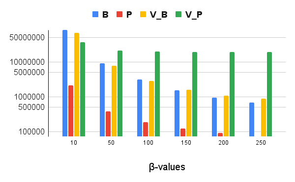
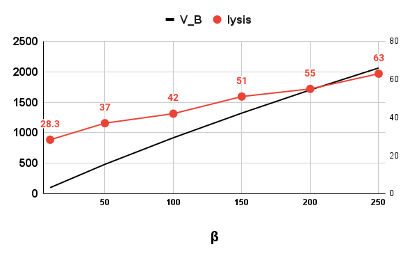
Figure 3: Variability of Phage Burst Size: Left - the maximum value of the biofilm cells $B$, planktonic cells $P$, Biofilm phage $V_{B}$ and the planktonic phage $V_{P}$, this is plotted for different values of the burst size $\beta$. Right - The minimum possible value of the biofilm phage for different burst size (black solid lines) is compared with the data from refr33 for different lysis time for comparable burst sizes (red) .

Stochastic Model - CTMC

If the bacteria (or phage) population is sufficiently small, an ordinary differential equation model is not appropriate, hence we utilize a continuous-time Markov chain (CTMC) model, which is continuous in time and discrete in the state space in order to study the variability at the initiation of bacteria clearance during phage treatment therapy, peak level of phage infection (in the phage-bacteria interaction, phages are seen as the pathogen and the bacteria are the susceptible). To make it simple, we use the same notation for the state variables as in the ordinary differential equation. The state variables are discrete random variables, $n,B,I,P\in\{0,1,2,3\}$ and $t\in[0,\infty]$

To formulate the CTMC, it is necessary to define the infinitesimal transition probabilities that corresponds to each event in the state variables, this is outlined in Table 2 which consists of $17$ distinct events.

Table 2: Table of transitions and corresponding probabilities in stochastic model

Table of events
Event	Event Description	Transitions	Change $\displaystyle(\Delta n,\Delta B,\Delta P,\Delta Vb,\Delta Vp,\Delta I)$	Probability
1	Availability of nutrient	$n\rightarrow n+1$	$(1,0,0,0,0,0)$	$f(n)\Delta t+o(\Delta t)$
2	Nutrient consumption and bacterial growth	$n\rightarrow n-1$	$(-1,1,0,0,0,0)$	$\left(\lambda_{B}B\right)\frac{n}{n+k}\Delta t+o(\Delta t)$
		$B\rightarrow B+1$
3	Nutrient consumption and bacterial growth	$n\rightarrow n-1$	$(-1,0,1,0,0,0)$	$\left(\lambda_{P}P\right)\frac{n}{n+k}\Delta t+o(\Delta t)$
		$P\rightarrow P+1$
4	Bacteria migration	$B\rightarrow B-1$	$(0,-1,+1,0,0,0)$	$(\gamma_{1}\frac{V_{B}}{\zeta_{1}+V_{B}}B)\Delta t+o(\Delta t)$
		$P\rightarrow P+1$
5	Bacteria migration	$P\rightarrow P-1$	$(0,1,-1,0,0,0)$	$(\gamma_{2}\frac{B}{\zeta_{2}+B}P)\Delta t+o(\Delta t)$
		$B\rightarrow B+1$
6	Biofilm Bacteria infection by phage	$B\rightarrow B-1$	$(0,-1,0,0,0,1)$	$(\phi_{1}BV_{B})\Delta t+o(\Delta t)$
		$I\rightarrow I+1$
7	Planktonic Bacteria infection by phage	$P\rightarrow P-1$	$(0,0,-1,0,0,1)$	$(\phi_{2}PV_{P})\Delta t+o(\Delta t)$
		$I\rightarrow I+1$
8	Biofilm-Phage Migration	$V_{B}\rightarrow V_{B}-1$	$(0,0,0,-1,1,0)$	$(qV_{B})\Delta t+o(\Delta t)$
		$V_{P}\rightarrow V_{P}+1$
9	Biofilm-Phage Migration	$V_{P}\rightarrow V_{P}-1$	$(0,0,0,1,-1,0)$	$(pV_{P})\Delta t+o(\Delta t)$
		$V_{P}\rightarrow V_{P}+1$
10	Biofilm-Phages gain from infected cells	$V_{B}\rightarrow V_{B}+1$	$(0,0,0,1,0,0)$	$(\beta\phi_{1}V_{B}B)\Delta t+o(\Delta t)$
11	Planktonic-Phages gain from infected cells	$V_{P}\rightarrow V_{P}+1$	$(0,0,0,0,1,0)$	$(\beta\phi_{2}V_{P}P)\Delta t+o(\Delta t)$
12	Death of Biofilm bacteria	$B\rightarrow B-1$	$(0,-1,0,0,0,0)$	$(\mu_{B}B)\Delta t+o(\Delta t)$
13	Death of Planktonic bacteria	$P\rightarrow P-1$	$(0,0,-1,0,0,0)$	$(\mu_{P}P)\Delta t+o(\Delta t)$
14	Biofilm-Phages death	$V_{P}\rightarrow V_{P}-1$	$(0,0,0,-1,0,0)$	$(c_{1}V_{B}B)\Delta t+o(\Delta t)$
15	Planktonic-Phages death	$V_{B}\rightarrow V_{B}-1$	$(0,0,0,-1,0,0)$	$(c_{2}V_{P}P)\Delta t+o(\Delta t)$
16	Decay of infected cells	$I\rightarrow I-1$	$(0,0,0,0,0,-1)$	$(\frac{10n}{\tau(n+k)})\Delta t+o(\Delta t)$
17	Death of infected cells	$I\rightarrow I-1$	$(0,0,0,0,0,-1)$	$(\alpha I)\Delta t+o(\Delta t)$

2.3.1 CTMC Analysis

For the continuous time markov chains, we numerically simulate the sample paths in order to determine the peak number of infected bacteria and peak phage-bacteria infection. For the sample paths, we simply compare our results with that of the ordinary differential equations.

Sample paths

An example of the sample paths that result from the Continuous Time Markov Chain model is shown in Figure 4 where the sample paths are captured by the red, blue, green and yellow, whereas the ODE model is captured by the black line. We observe that these sample paths generally aligned with the population average response that is captured by the ODE model. The sample paths of the CTMC model show the potential variability in timing of the peak level of infection and the peak number of infected bacteria. Due to limitation in computational memory, we reduced the initial values of the dependent variables as shown in Table 2; in other words, we have used the following initial conditions $n_{0}=10^{5}gm^{-3},B_{0}=10^{4}gm^{-3},P_{0}=0,V_{B0}=10^{3}gm^{-3},V_{P0}=0,I_{0}=0$

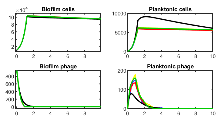
Figure 4: Sample Paths This is the sample paths to the CMTC model, due to insufficient memory space, we used a reduced initial conditions for all the dependent variables, that is $1e5,1e2,0,1e3,0,0$ corresponding to $n_{0},B_{0},P_{0},Vb_{0},Vp_{0},I_{0}$ respectively

Time to Peak Infection and Peak Number of Infected Biofilm Bacteria

We asked whether bacteria infection will reach peak infection in a shorter time, to investigate this, we calculated the mean ($\pm$ SD) of time to peak infection for the bacteria in the biofilm. This is presented in Figure 5 showing that we can attend peak infection with just one phage in the system within a limited time. By introducing few bacteriophages, we observed a large amount of infected bacterial cells resulting from the interaction, this shows that there were a large replication of the viruses. Interestingly, this happened within a short period of time. Even though we do not know how long it might take phage therapy to work, experimental data have shown that treatment of bacteria infection could be achieved in a period as short as $10$ days and up to $8$ weeks refr38 , this is in agreement with our finding.

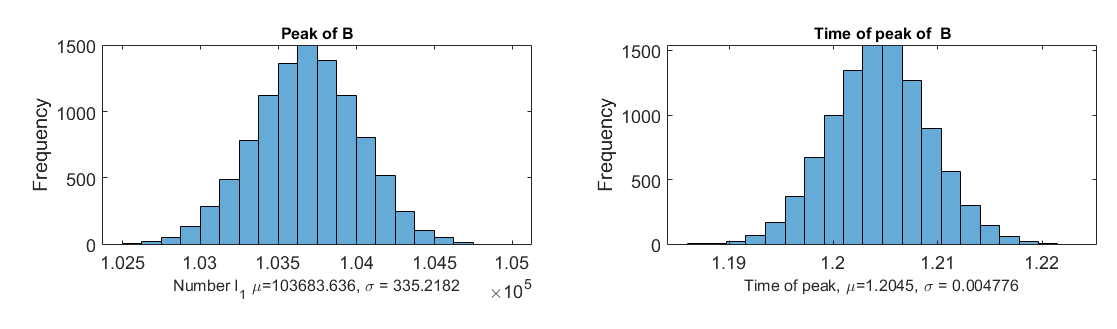
Figure 5: Peak Infection This shows the peak infection of bacteria (left) and the corresponding time to reach the peak infection (right).

3 Parameter Sensitivity Analysis

We perform a sensitivity analysis on the parameters ranges given in Table 3 for the ODE models using a uniform distribution for the values. Latin hypercube sampling (LHS), first developed by McKay et al. refr31 ; refr34 , with the statistical sensitivity measure partial rank correlation coefficient (PRCC), performs a sensitivity analysis that explores a defined parameter space of the model. The parameter space considered is defined by the parameter intervals depicted in Table 3. Rather than simply exploring one parameter at a time with other parameters held fixed at baseline values, the LHS/PRCC sensitivity analysis method globally explores multidimensional parameter space. LHS is a stratified Monte Carlo sampling without replacement technique that allows an unbiased estimate of the average model output with limited samples. The PRCC sensitivity analysis technique works well for parameters that have a nonlinear and monotonic relationship with the output measure. The PRCC presented in Figure 6 shows how the output measure is influenced by changes in a specific parameter value when the linear effects of other parameter values are removed. The PRCC values were calculated as Spearman (rank) partial correlations using the partialcorr function in MATLAB 2020. Their significance, uncorrelated p-values, were also determined. The PRCC values vary between $-1$ and $1$, where negative values indicate that the parameter is inversely proportional to the outcome measure. Following Marino et al. refr35 , we performed a z-test on transformed PRCC values to rank significant model parameters in terms of relative sensitivity. According to the z-test, parameters with larger magnitude values had a stronger effect on the output measures.

We start by verifying the monotonicity of the output measures. Monotonicity was observed for all parameters, hence we use PRCC. PRCC analysis of these ranges produces similar results. For the biofilm-phage model, we calculate the PRCC for the following output measures: infected bacteria cells, bacteriophages in the planktonic phase and 10% population of infected bacteria cells.

	Parameter	Values
		Baseline	Range
$\lambda_{B}$	biofilm bacteria growth rate	0.06
$\lambda_{P}$	planktonic bacteria growth rate	0.6931∗∗	(0.4, 0.8)
$k$	Monod constant	6.3	(2-8)
$\gamma_{1}$	phage induced detachment rate	0.4	(0.1, 2)
$\gamma_{2}$	natural detachment rate	0.08	(0.02, 0.14)
$\phi_{1}$	biofilm predation rate	0.075	(0.05, 0.1)
$\phi_{2}$	planktonic predation rate	0.075	(0.05, 0.1)
$\zeta_{1}$	Monod saturation	0.075	(0.05, 0.1)
$\zeta_{2}$	Monod saturation	0.075	(0.05, 0.1)
$c_{1}$	biofilm phage lysis	0.075	(0.05, 0.1)
$c_{2}$	planktonic phage lysis	0.075	(0.05, 0.1)
$p$	phage detachment rate	6.3	(2-8)
$q$	phage reattachment rate	6.3	(2-8)
$\tau$	Average latency time	6.3	(2-8)
$b$	Burst size	6.3	(2-8)
$\alpha$	Infection decay rate	6.3	(2-8)

Table 3: Baseline parameter values are used in all simulations. The range of values presented in this table is used for the parameter sensitivity analysis

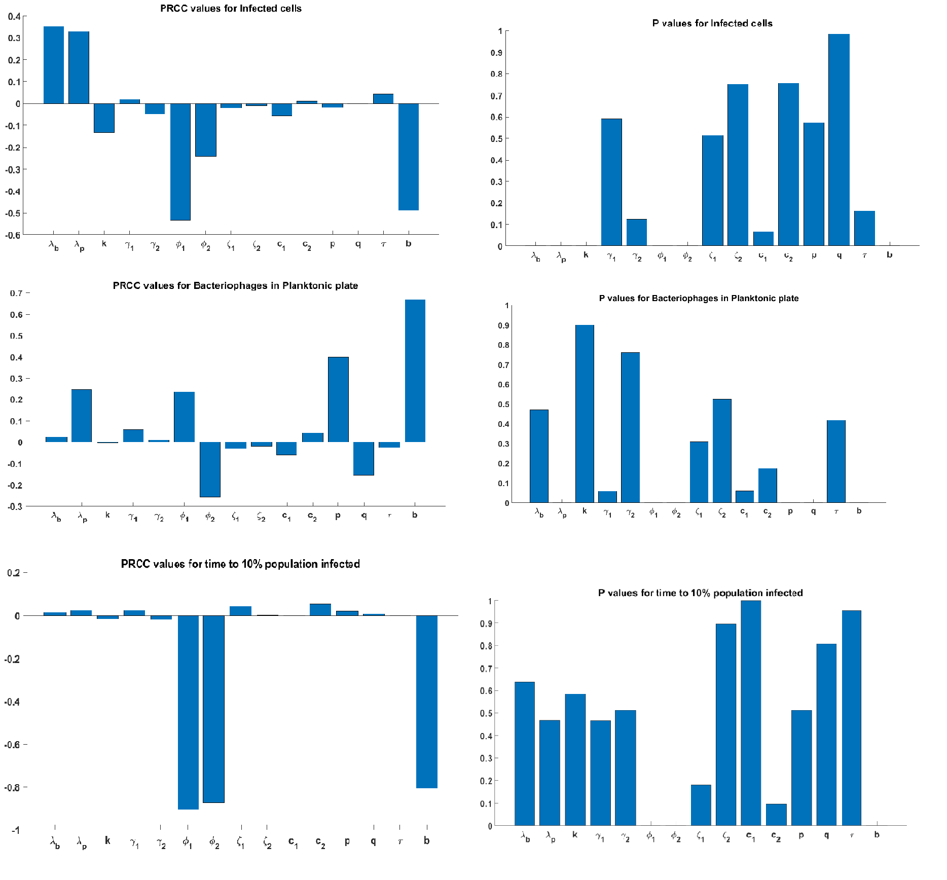
Figure 6: PRCC This is the partial rank correlation coefficient for the sensitivity analysis of the parameters

4 Discussion

We have developed a bacteria-phage interaction model within a biofilm in a cystic fibrosis patient. The model considers bacteria in a biofilm and planktonic phase. The model assumes that the interactions are region-specific, which means that the phages in the planktonic phase can only interact with the planktonic bacteria while the phages in the biofilm can only interact with biofilm bacteria cells. The model speculates that the burst size could control the biofilm growth. In an effort to understand the state of the disease over time, we developed a stochastic model with which we could investigate the probabilities of reaching peak infection within a short time.

The model in this study can be easily adopted to investigate the effect of factors such as temperature and pH value on middle ear infection. Experimental study in osgood ; osgoodref revealed that the pH of middle ear fluid collected from acute otitis media of children could affect biofilm formation, and biofilm formation is limited or completely absent under aerobic conditions as likely to happen, therefore the current model in this study can be adopted with the inclusion of these specific factors to understand the interaction of phages and bacteria in middle ear infection.

Our assumptions and findings are consistent with the dynamics associated with biofilms. For instance, one of our main assumptions confirms that the phage interaction rate in the biofilm is different from the planktonic since the bacteria in the biofilm are dense and encased with extracellular polymeric substances, this is consistent with several in vitro settings refr6 ; refr13 ; refr17 ; refr18 ; refr19 ; refr36 ; refr37 .

In connecting models to experiment, our model is not able to explain the biofilm occupancy which will require the spatial components incorporated into the model, the spatial structures can definitely be therapeutically relevant. For example, understanding the biofilm matrix and EPS will help to understand the actual interaction rates within the biofilm; the bacteria occupancy in the biofilm will help to determine if the phage interactions is at the biofilm surface, mimicking a lollipop-like degradation, or from within the biofilm, thus forming cavities. Another extension of this model are to: (a) investigate a combination therapy that will involve antibiotics and immune response, (b) investigate the factors that influence biofilm formation and how they can be manipulated to prevent and eliminate biofilm-associated diseases in other areas of the body.

References

- (1) Emerenini, BO, Williams , Reyes Grimaldo RNG , Wurscher K, and Ijioma R. 2021. Mathematical Modeling and Analysis of Influenza In-Host Infection Dynamics. Letters in Biomathematics 8 (1), 229–253.https://doi.org/10.30707/LiB8.1.1647878866.124006.
- (2) Musk Jr DJ, Hergenrother PJ. Chemical countermeasures for the control of bacterial biofilms: effective compounds and promising targets. Current medicinal chemistry. 2006 Aug 1;13(18):2163-2177.https://doi.org/10.2174/092986706777935212
- (3) Potera C. Phage renaissance: new hope against antibiotic resistance. Environmental Health Perspectives. 2013 Feb 1;121(2):A48-A53. https://doi.org/10.1289/ehp.121-a48
- (4) Carlton RM. Phage therapy: past history and future prospects. Archivum Immunologiae et Therapiae Experimentalis-English Edition. 1999 Sep;47:267-274.
- (5) Bañuelos, S., Gulbudak, H., Horn, M.A., Huang, Q., Nandi, A., Ryu, H., and Segal, R.A. (2020). Investigating the impact of combination phage and antibiotic therapy: a modeling study. bioRxiv.
- (6) Loc-Carrillo C, Abedon ST. Pros and cons of phage therapy. Bacteriophage. 2011 Mar 1;1(2):111-114.https://doi.org/10.4161/bact.1.2.14590
- (7) Dkabrowska K, Abedon ST. Pharmacologically aware phage therapy: pharmacodynamic and pharmacokinetic obstacles to phage antibacterial action in animal and human bodies. Microbiology and Molecular Biology Reviews. 2019 Oct 30;83(4):e00012-19.https://doi.org/10.1128/MMBR.00012-19
- (8) Siettos CI, Russo L. Mathematical modeling of infectious disease dynamics. Virulence. 2013 May 15;4(4):295-306.https://doi.org/10.4161/viru.24041
- (9) Kermack WO, McKendrick AG. A contribution to the mathematical theory of epidemics. Proceedings of the royal society of london. Series A, Containing papers of a mathematical and physical character. 1927 Aug 1;115(772):700-721. https://doi.org/10.1098/rspa.1927.0118
- (10) Ross R. The prevention of malaria. Second Edition. John Murray; 1911.
- (11) Anderson RM, May RM. Infectious diseases of humans: dynamics and control. Oxford university press; 1992 Aug 27.
- (12) Dieckmann U. Adaptive dynamics of pathogen-host interactions. In Adaptive Dynamics of Infectious Diseases: In Pursuit of Virulence Management. Cambridge Studies in Adaptive Dynamics. Cambridge University Press. 2002 (pp 39-59). ISBN 978-0-521-78165-7
- (13) Ewald J, Sieber P, Garde R, Lang SN, Schuster S, Ibrahim B. Trends in mathematical modeling of host-pathogen interactions. Cellular and Molecular Life Sciences. 2020 Feb;77(3):467-80.https://doi.org/10.1007/s00018-019-03382-0
- (14) Keeling MJ, Rohani P. Modelling Infectious Diseases in Humans and Animals. Princeton, NJ: Princeton University Press. 2008.
- (15) Beke G, Stano M, Klucar L. Modelling the interaction between bacteriophages and their bacterial hosts. Mathematical Biosciences. 2016 Sep 1;279:27-32.https://doi.org/10.1016/j.mbs.2016.06.009
- (16) Bardina C, Spricigo DA, Cortés P, Llagostera M. Significance of the bacteriophage treatment schedule in reducing Salmonella colonization of poultry. Applied and environmental microbiology. 2012 Sep 15;78(18):6600-7. https://doi.org/10.1128/AEM.01257-12
- (17) Sinha S, Grewal RK, Roy S. Modeling Phage-Bacteria Dynamics. In Immunoinformatics. Methods in Molecular Biology, Vol. 2131. 2020 (pp. 309-327). Humana, New York, NY.https://doi.org/10.1007/978-1-0716-0389-5_18
- (18) Emerenini BO, Hense BA, Kuttler C, Eberl HJ. A mathematical model of quorum sensing induced biofilm detachment. PloS one. 2015 Jul 21;10(7):e0132385. https://doi.org/10.1371/journal.pone.0132385
- (19) Emerenini BO, Eberl HJ. Reactor scale modeling of quorum sensing induced biofilm dispersal. Appl. Math. Comput.2022,418, 12679
- (20) D’Acunto B, Frunzo L, Klapper I, Mattei MR, Stoodley P. Mathematical modeling of dispersal phenomenon in biofilms. Mathematical biosciences. 2019 Jan 1;307:70-87.https://doi.org/10.1016/j.mbs.2018.07.009
- (21) Hughes KA, Sutherland IW, Jones MV. Biofilm susceptibility to bacteriophage attack: the role of phage-borne polysaccharide depolymerase. Microbiology. 1998 Nov 1;144(11):3039-3047.https://doi.org/10.1099/00221287-144-11-3039
- (22) Brüssow H. Bacteriophage-host interaction: from splendid isolation into a messy reality. Current opinion in microbiology. 2013 Aug 1;16(4):500-506. https://doi.org/10.1016/j.mib.2013.04.007
- (23) Eriksen RS, Mitarai N, Sneppen K. Sustainability of spatially distributed bacteria-phage systems. Scientific reports. 2020 Feb 21;10(1):1-2. https://doi.org/10.1038/s41598-020-59635-7
- (24) De Paepe M, Taddei F. Viruses’ life history: towards a mechanistic basis of a trade-off between survival and reproduction among phages. PLoS biology. 2006 Jul;4(7):e193.https://doi.org/10.1371/journal.pbio.0040193
- (25) Donlan RM. Preventing biofilms of clinically relevant organisms using bacteriophage. Trends in microbiology. 2009 Feb 1;17(2):66-72. https://doi.org/10.1016/j.tim.2008.11.002
- (26) Sillankorva S, Oliveira R, Vieira MJ, Sutherland I, Azeredo J. Bacteriophage S1 infection of Pseudomonas fluorescens planktonic cells versus biofilms. Biofouling. 2004 May 1;20(3):133-138. https://doi.org/10.1080/08927010410001723834
- (27) Hadas H, Einav M, Fishov I, Zaritsky A. Bacteriophage T4 development depends on the physiology of its host Escherichia coli. Microbiology. 1997 Jan 1;143(1):179-85.https://doi.org/10.1099/00221287-143-1-179
- (28) Parasion S, Kwiatek M, Gryko R, Mizak L, Malm A. Bacteriophages as an alternative strategy for fighting biofilm development. Polish Journal of Microbiology. 2014 Feb 6;63(2):137-145.
- (29) Cerca N, Oliveira R, Azeredo J. Susceptibility of Staphylococcus epidermidis planktonic cells and biofilms to the lytic action of staphylococcus bacteriophage K. Letters in applied microbiology. 2007 Sep;45(3):313-317. https://doi.org/10.1111/j.1472-765X.2007.02190.x
- (30) Jamal M, Hussain T, Das CR, Andleeb S. Characterization of Siphoviridae phage Z and studying its efficacy against multidrug-resistant Klebsiella pneumoniae planktonic cells and biofilm. Journal of medical microbiology. 2015 Apr 1;64(4):454-462.https://doi.org/10.1099/jmm.0.000040
- (31) Hanlon GW, Denyer SP, Olliff CJ, Ibrahim LJ. Reduction in exopolysaccharide viscosity as an aid to bacteriophage penetration through Pseudomonas aeruginosa biofilms. Applied and environmental microbiology. 2001 Jun 1;67(6):2746-2753.https://doi.org/10.1128/AEM.67.6.2746-2753.2001
- (32) Hosseinidoust Z, Tufenkji N, van de Ven TG. Formation of biofilms under phage predation: considerations concerning a biofilm increase. Biofouling. 2013 Apr 1;29(4):457-468.https://doi.org/10.1080/08927014.2013.779370
- (33) Ellis EL, Delbruck M. The growth of bacteriophage. The Journal of general physiology. 1939 Jan 20;22(3):365-384.https://doi.org/10.1085/jgp.22.3.365
- (34) Delbrück M. The growth of bacteriophage and lysis of the host. The journal of general physiology. 1940 May 5;23(5):643-660. https://doi.org/10.1085/jgp.23.5.643
- (35) McKay MD. Latin hypercube sampling as a tool in uncertainty analysis of computer models. In Proceedings of the 24th conference on Winter simulation 1992 Dec 1 (pp. 557-564).
- (36) De Paepe M, Taddei F. Viruses’ life history: towards a mechanistic basis of a trade-off between survival and reproduction among phages. PLoS biology. 2006 Jul;4(7):e193.https://doi.org/10.1371/journal.pbio.0040193
- (37) Wang IN. Lysis timing and bacteriophage fitness. Genetics. 2006 Jan 1;172(1):17-26.https://doi.org/10.1534/genetics.105.045922
- (38) Ng RN, Tai AS, Chang BJ, Stick SM and Kicic A Overcoming Challenges to Make Bacteriophage Therapy Standard Clinical Treatment Practice for Cystic Fibrosis. (2021) Front. Microbiol. 11:593988. doi: 10.3389/fmicb.2020.593988
- (39) McKay MD, Beckman RJ, Conover WJ. A comparison of three methods for selecting values of input variables in the analysis of output from a computer code. Technometrics. 2000 Feb 1;42(1):55-61.http://doi.org/10.1080/00401706.2000.10485979
- (40) Marino S, Hogue IB, Ray CJ, Kirschner DE. A methodology for performing global uncertainty and sensitivity analysis in systems biology. Journal of theoretical biology. 2008 Sep 7;254(1):178-96.https://doi.org/10.1016/j.jtbi.2008.04.011
- (41) Osgood R, Salamone F, Diaz A, Casey JR, Bajorski P, Pichichero ME. Effect of pH and oxygen on biofilm formation in acute otitis media associated NTHi clinical isolates. Laryngoscope. 2015 Sep;125(9):2204-8. doi: 10.1002/lary.25102. Epub 2015 May 13. PMID: 25970856.
- (42) Wright A, Hawkins CH, Anggård EE, Harper DR. A controlled clinical trial of a therapeutic bacteriophage preparation in chronic otitis due to antibiotic-resistant Pseudomonas aeruginosa; a preliminary report of efficacy. Clin Otolaryngol. 2009 Aug;34(4):349-57. doi: 10.1111/j.1749-4486.2009.01973.x. PMID: 19673983.
- (43) Waters EM, Neill DR, Kaman B, Sahota JS, Clokie MR, Winstanley C, Kadioglu A. Phage therapy is highly effective against chronic lung infections with Pseudomonas aeruginosa. Thorax. 2017 Jul 1;72(7):666-667. http://dx.doi.org/10.1136/thoraxjnl-2016-209265
- (44) Bjarnsholt T. The role of bacterial biofilms in chronic infections. Apmis. 2013 May;121:1-58.