Broadcasting in random recursive dags

Abstract

A uniform $k$-dag generalizes the uniform random recursive tree by picking $k$ parents uniformly at random from the existing nodes. It starts with $k$ ”roots”. Each of the $k$ roots is assigned a bit. These bits are propagated by a noisy channel. The parents’ bits are flipped with probability $p$, and a majority vote is taken. When all nodes have received their bits, the $k$-dag is shown without identifying the roots. The goal is to estimate the majority bit among the roots. We identify the threshold for $p$ as a function of $k$ below which the majority rule among all nodes yields an error $c+o(1)$ with $c<1/2$. Above the threshold the majority rule errs with probability $1/2+o(1)$.

1 Introduction

The interest in network analysis has been growing, in part due to its use in communication technologies, social network studies, and biology, see Coolen et al. [5]. The problem we study here is the one of broadcasting on random graphs. We study the setting where a bit propagates with noise and we want to infer the value of the original bit. The question is not if and how the information propagates, but if there is a signal propagating on the graph, or only noise. Variations of this binary classification problem have been studied. For example, in the root-bit estimation problem, the root of a tree has a bit $0$ or $1$. The value of this bit propagates from the root to the leafs, and at each propagation from a vertex to the next it mutates (flips the bit) with probability $p$. One can try to infer the root’s bit value from observing all the bits of the graph or only the leaf bits. This question was first formulated in Evans et al. [8] on general trees, where it was shown that root bit reconstruction is possible depending upon a condition on the branching number. More recently, the case of random recursive trees (Addario-Berry et al. [1], Desmarais et al. [7]) has been studied. Other variations of these problems on trees include looking at asymmetric flip probabilities (Sly [20]), non-binary vertex values (Mossel [16]) and robustness to perturbation (Janson and Mossel [12]). We refer the reader to Mossel [17] for a survey of reconstruction problems on trees. Many problems are described by more general graphs rather than trees. The original broadcasting question has been studied on deterministic graphs (Harutyunyan and Li [9]) and Harary graphs (Bhabak et al. [3], for example). We are interested in the problem of noisy propagation in the spirit of the root-bit reconstruction (Evans et al. [8]), but on a class of random graphs that we call $k$-dag (for directed acyclic graph). A similar problem – for a different class of random dags – has been studied in Makur et al. [15].

Since we track the proportion of zero bits in our graph, we cast the process as an urn model. A similar reformulation was already done in Addario-Berry et al. [1] to study majority voting properties of broadcasting on random recursive trees. The proportion of zero bits and the bit assignment procedure can be viewed as random processes with reinforcement. A review of results can be found in Pemantle [19] and is extensively used, alongside results of non-convergence found in Pemantle [18]. As in Addario-Berry et al. [1], we make ample use of the properties of Pólya urns (Wei [21], Janson [10], Knape and Neininger [13]). Variations of the Pólya urn model that are useful for our analysis include an increase of the number of colors over time (Bertoin [2]), the selection of multiple balls in each draw (Kuba and Mahmoud [14]), and randomization in the color of the new ball (Janson [11], Zhang [22]). We note, in particular, the multi-ball draw with a linear randomized replacement rule of Crimaldi et al. [6]. In the present paper, we consider multi-ball draws, but with non-linear randomized replacement.

The paper is organized as follows. After introducing the mathematical model in Section 1.1, in Section 1.2 we present the main result of the paper (Theorem 1) that shows that there are three different regimes of the value of the mutation probability that characterize the asymptotic behavior of the majority rule. In Section 2 we discuss the three regimes of $p$. In Section 3 we establish convergence properties of the global proportion of both bit values assigned to vertices and in Section 4 we finish the proof of Theorem 1 by studying the probability of error in all three regimes. Finally, in Section 5 we establish a lower bound for the probability of error that holds uniformly for all mutation probabilities. We conclude the paper by discussing avenues for further research.

1.1 The model

We start by describing the evolution of the uniform random recursive $k$-dag and the assigned bit values that we represent by two colors; red and blue.

Let us fix an odd integer $k>0$. The growth process is initiated at time $k$. At time $k$, the graph consists of $k$ isolated vertices. A fraction $R_{k}$ are red and a fraction $B_{k}=1-R_{k}$ are blue. We set $R_{1}=\cdots=R_{k}$ and $B_{1}=\cdots=B_{k}$. The network is grown recursively by adding a new colored vertex and at most $k$ edges at each time step. At time $n$, a new vertex $n$ connects to a sample of $k$ vertices chosen uniformly at random with replacement among the $n-1$ previous vertices. (Possible multiple edges are collapsed into one so that the graph remains simple.) The color of vertex $n$ is determined by the following randomized rule:

• the colors of the $k$ selected parents are observed;

• each of these is independently flipped with probability $p$ (if a parent is selected more than once, its color is flipped independently for each selection);

• the color of vertex $n$ is chosen according to the majority vote of the flipped parent colors.

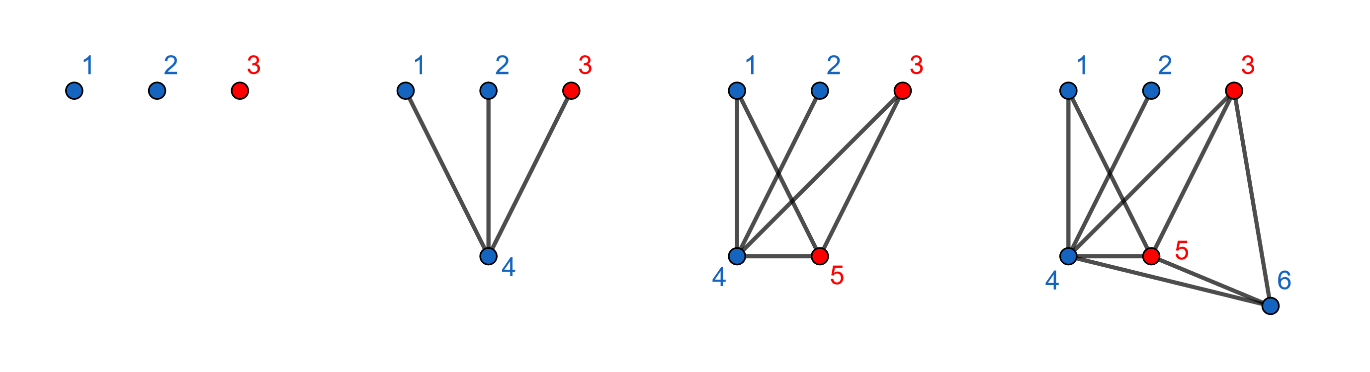
Figure 1: A realisation of the process up to time 6, for $k=3$, starting with $R_{3}=1/3$.

If one is only interested in the evolution of the proportion of red and blue vertices (but not the structure of the graph), one may equivalently describe it by an urn model with multiple draws and random (nonlinear) replacement. The urn process is defined as follows. The urn is initialized with an odd number $k$ of balls, a fraction $R_{k}$ being red and $B_{k}=1-R_{k}$ blue. At each time $n\geq k+1,$

• $k$ balls are drawn from the urn, uniformly at random, with replacement, and returned to the urn;

• the color of each ball is independently flipped with probability $p$;

• a new ball is added to the urn whose color is chosen as the majority of the flipped colors.

In the root-bit estimation problem considered here, the statistician has access to an unlabelled and undirected version of the graph at time $n$, along with the vertex colors. The goal of the statistician is to estimate the colors assigned to the $k$ roots. More precisely, based on the observed graph, one would like to guess the majority color at time $k$.

This problem has been studied in depth by [1] in the case when $k=1$, that is, when the produced graph is a uniform random recursive tree. Two types of methods for root-bit estimation were studied in [1]. One is based on first trying to localize the root of the tree–disregarding the vertex colors. If one finds a vertex that is close to the root, one may use the color of that vertex as a guess for the root color. Such a vertex is the centroid of the tree. Indeed, it is shown in [1] that the color of the centroid is a nearly optimal estimate of the root color. In the same paper, the majority rule is also studied. This method disregards the structure of the tree and guesses the root color by taking a majority vote among all vertices. It is shown that for small mutation probabilities the majority rule is also nearly optimal.

In the more general problem considered in this paper, one may also try to estimate the colors of the $k$ roots by finding nearby vertices. However, this problem becomes significantly more challenging as the $k$-dag does not have a natural centroid. The interested reader is referred to the recent paper of Briend, Calvillo, and Lugosi [4] on root finding in random $k$-dags. Instead of pursuing this direction, we focus on the majority vote. More precisely, we are interested in characterizing the values of the mutation probability $p$ such that the asymptotic probability of error is strictly better than random guessing.

At time $n$, the majority vote, denoted by $b^{maj}_{n}$, is defined as follows:

$$b^{maj}_{n}\ =\ \begin{cases}&\text{``R'' (red) if }R_{n}>1/2\\ \\ &\text{``B''(blue) if }R_{n}<1/2\\ \\ &\text{Ber}(1/2)\text{ if }R_{n}=1/2\text{ (a random coin flip)}~{}.\end{cases}$$

We define the probability of error by

$$R^{maj}(n,p)=\mathbb{P}\left\{b^{maj}_{n}\neq b^{maj}_{k}\right\}~{}.$$

Note that $b^{maj}_{k}$ depends on the initial vertex colors that are assumed to be chosen arbitrarily. Hence, $R^{maj}(n,p)$ is a function of the initial proportion $R_{k}$ but to avoid heavy notation, we supress this dependence.

1.2 Related results and our contribution

Our broadcasting model is an extension of the broadcasting on uniform random recursive trees that was extensively studied in Addario-Berry et al. [1]. In this problem, $k=1$ and the only parameter is $p$, the mutation probability. For the majority voting rule, they prove the following:

1. There exists a constant $c>0$ such that

   $$\limsup_{n\to\infty}R^{maj}(n,p)\leq cp~{}.$$

2. For all $p\in(0,1/2]$,

   $$\lim_{n\to\infty}R_{n}=\frac{1}{2}\quad\text{with probability one}~{}.$$

3. For $p\in[0,1/4)$

   $$\limsup_{n\to\infty}R^{maj}(n,p)<\frac{1}{2}~{}.$$

4. For $p\in[1/4,1/2]$

   $$\limsup_{n\to\infty}R^{maj}(n,p)=\frac{1}{2}~{}.$$

In other words, even though the proportion of vertices that have the same color as the root converges to $1/2$, for mutation probabilities smaller than $1/4$, sufficient information is preserved about the root color for the majority vote to work with a nontrivial probability.

We generalize these results to $k$-dags and characterize the values of $p$ for which majority voting outperforms random guessing. In order to state the main result of the paper, we introduce some notation.

For any odd positive integer $k$, let

$$\alpha_{k}:=\frac{1}{2^{k-2}}\sum_{i>k/2}^{k}\binom{k}{i}(i-k/2)=\mathbb{E}\left[\left(Bin(k,1/2)-\frac{k}{2}\right)_{+}\right]~{}.$$ (1.1)

For example, $\alpha_{1}=1$, $\alpha_{3}=3/2$, and by an simple application of the central limit theorem, for large $k$,

$$\alpha_{k}\sim\sqrt{\frac{2k}{\pi}}~{}.$$ (1.2)

In the statement of our main theorem, we assume, without loss of generality, that initially red vertices are in majority, that is, $R_{k}>1/2$.

Theorem 1 shows that for all $k\geq 3$, there are three regimes of the value of the mutation probability. In the low-rate-of-mutation regime the proportion of red balls almost surely converges to one of two numbers, both different from $1/2$. Moreover, the limiting proportion is positively correlated with the initial value. In the intermediate phase, the vertex colors are asymptotically balanced, but there is enough signal for the majority vote to perform strictly better than random guessing. Finally, in the high-rate-of-mutation regime, the majority vote is equivalent to a coin toss, at least asymptotically.

Note that for $k=1$, $\alpha_{1}=1$, so $1/2-1/(2\alpha_{1})=0$, and therefore the low-rate-of-mutation regime does not exist. Of course, this is in accordance with the results of [1] cited above.

On the other hand, for $k=3$ the two thresholds are $1/2-1/(2\alpha_{3})=1/6$ and $1/2-1/(4\alpha_{1})=1/3$, meaning that from $k=3$ onward the three different regimes can be observed. For large $k$, both threshold values are of the order $1/2-\Theta(1/\sqrt{k})$.

A closely related model has been studied by Makur et al. [15]. They study different random dags, where important parameters are the number of vertices at distance $k$ from the root and the indegree of vertices. They also suppose that the position of the root vertex is known. Two rules of root bit estimation are studied: a noisy majority rule and the NAND rule. Makur et al. [15] show that if the number of vertices of depth $k$ is $\Omega\left(\log(k)\right)$ then there is a threshold on the mutation probability for which root bit estimation is possible.

As a first step, we study the convergence of the proportion of red balls. To this end, it suffices to study the generalized urn process defined above. We mention here that Crimaldi et al. [6] study a somewhat related urn process, though with linear replacement rules.

2 Different regimes

We start by studying the evolution of $R_{n}$. Let us denote by $c_{n}$ the color of the $n$-th vertex appearing in the graph. After possible mutation, each edge connecting vertex $n+1$ to an older vertex carries a signal. This signal is red with probability

$$f(R_{n}):=(1-p)R_{n}+p(1-R_{n})=(1-2p)R_{n}+p~{}.$$

Because the $k$ parents are chosen independently and that the color is chosen by the majority,

$$\mathbb{P}\left\{c_{n+1}=R\right\}\ =\ \mathbb{P}\left\{\text{Bin}\left(k,f(R_{n})\right)\geq k/2\right\}~{},$$ (2.1)

where, conditionally on $R_{n}$, $\text{Bin}\left(k,f(R_{n})\right)$ is a binomial random variable. Moreover, we know that the number of red vertices evolves as $(n+1)R_{n+1}=nR_{n}+\mathbbm{1}(c_{n+1}=R)$, where $\mathbbm{1}$ is the indicator function. We rewrite this as

$$R_{n+1}=R_{n}+\frac{\mathbbm{1}(c_{n+1}=R)-R_{n}}{n+1}~{}.$$ (2.2)

A key to understanding $R_{n}$ is then to study the random variable $\mathbbm{1}(c_{n+1}=R)-R_{n}$. We define, for $t\in[0,1]$,

$$g(t)\ :=\ \mathbb{E}\left[\mathbbm{1}(c_{n+1}=R)-R_{n}|R_{n}=t\right]\ =\mathbb{P}\left\{\text{Bin}(k,f(t))>k/2\right\}-t~{}.$$ (2.3)

The evolution of $R_{n}$ is entirely determined by the function $g$. Observe first that for any $t\in[0,1]$, $f(1-t)=1-f(t)$. Also, since $k$ is odd,

$$\mathbb{P}\left\{\text{Bin}(k,1-f(t))>k/2\right\}=1-\mathbb{P}\left\{\text{Bin}(k,f(t))>k/2\right\}~{},$$

which implies that

$$g(1-t)=-g(t)~{}.$$

The extremal values of $g$ are

$$g(0)=\mathbb{P}\left\{\text{Bin}(k,p)>k/2\right\}>0~{},$$

and

$$g(1)=\mathbb{P}\left\{\text{Bin}(k,1-p)>k/2\right\}-1<0~{}.$$

Since $g$ is continuous, the polynomial $g$ has at least one root. From the symmetry property we have $g(1/2)=-g(1-1/2)=-g(1/2)$, so $g(1/2)=0$. Moreover we obtain

$$g^{\prime}(1/2)=\frac{1-2p}{2^{k-2}}\sum_{i>k/2}^{k}\binom{k}{i}(i-k/2)-1~{}.$$

Recalling the definition of $\alpha_{k}$ from (1.1), we have $g^{\prime}(1/2)=(1-2p)\alpha_{k}-1$. Since $\alpha_{k}\geq 1$, we conclude:

$$g^{\prime}\left(\frac{1}{2}\right)\ \begin{cases}\ <0&\text{if }p>\frac{1}{2}-\frac{1}{2\alpha_{k}}~{},\\ \\ \ >0&\text{if }p<\frac{1}{2}-\frac{1}{2\alpha_{k}}~{}.\end{cases}$$

To understand the other potential zeros of $g$, let us study its convexity. We may use the elementary identities

$$\mathbb{P}\left\{\text{Bin}(k,x)\geq\frac{k+1}{2}\right\}=\mathbb{P}\left\{\text{Beta}\left(\frac{k+1}{2},\frac{k+1}{2}\right)<x\right\}~{},$$ (2.4)

where Beta$(a,b)$ is a beta$(a,b)$ random variable. Hence,

$$g(t)=\int_{0}^{f(t)}\left(x(1-x)\right)^{\frac{k-1}{2}}\frac{\Gamma(k+1)}{\Gamma^{2}\left(\frac{k+1}{2}\right)}dx\ \ -t~{},$$

and therefore

$$g^{\prime}(t)=(1-2p)\left(f(t)(1-f(t))\right)^{\frac{k-1}{2}}\frac{\Gamma(k+1)}{\Gamma^{2}\left(\frac{k+1}{2}\right)}-1~{}.$$ (2.5)

Since $f(t)(1-f(t))=-(1-2p)t(t-1)+p(1-p)$ is increasing for $t\in(0,1/2)$ and decreasing for $t\in(1/2,1)$, $g$ is strictly convex on $(0,1/2)$ and strictly concave on $(1/2,1)$.

In summary, if $p>\frac{1}{2}-\frac{1}{2\alpha_{k}}$, then $g^{\prime}(1/2)<0$, and thus $g$ is monotonically decreasing on $[0,1]$ and has only one zero in $[0,1]$. If $g^{\prime}(1/2)=0$, then there is only one zero (at $1/2$) and $g$ exhibits an inflection point at $1/2$. If $p<\frac{1}{2}-\frac{1}{2\alpha_{k}}$, then $g^{\prime}(1/2)>0$ and thus $g$ has exactly one zero in $(0,1/2)$ and by symmetry, it also has one zero on $(1/2,1)$. We denote these zeros by $\beta_{1}$ and $\beta_{2}$, respectively.

Figure 2 shows two examples of the graph of the function $g$.

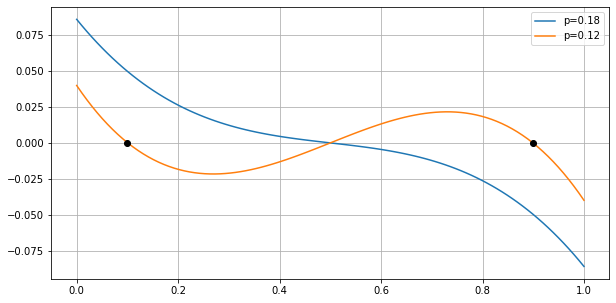
Figure 2: $g$ as a function of $t\in[0,1]$, for $k=3$, with the choices $p=0.18>1/6$ and $p=0.12<1/6$.

It is also interesting to know the position of $\beta_{1}$ (recall that $\beta_{2}=1-\beta_{1}$). First, we note that for fixed $k$, if $p$ tends to the threshold $1-1/(2\alpha_{k})$, then $\beta_{1}$ tends to $1/2$. We study the case when $p$ is far enough from the threshold, that is, when $p\leq\frac{1}{2}-\frac{C}{2\alpha_{k}}$, for some large constant $C$. $\beta_{1}$ is the smallest root of $g(t)$ and since $g(0)>0$, its smallest root is smaller than the smallest root of any upper bound of $g$. On the other hand,

$$g(t)=\mathbb{P}\left\{\text{Bin}(k,f(t))\geq\frac{k}{2}\right\}-t\leq\exp\left(-2k\left(\frac{1}{2}-f(t)\right)^{2}\right)=\exp\left(-2k(1-2p)^{2}\left(\frac{1}{2}-t\right)^{2}\right)-t~{}.$$

Thus, $\beta_{1}$ is at most the first zero of $b(t):=\exp\left(c_{1}\left(\frac{1}{2}-t\right)^{2}\right)-t$, for $c_{1}=2k(1-2p)^{2}$. Since $b(0)>0$, if for some $t^{*}$, $b(t^{*})\leq 0$ then the first zero of $b$ and therefore $\beta_{1}$ is at most $t^{*}$. Taking $t^{*}=e^{-c_{1}/16}$, we have

$$b(t^{*})\leq 0\iff\left(\frac{1}{2}-e^{-c_{1}/16}\right)^{2}\geq 1/16\iff c_{1}\geq 32\log(2)~{}.$$

From (1.2) and the expression of $c_{1}$, we have that by taking $C\geq\sqrt{\frac{8\log(2)}{\pi}}$,

$$2k(1-2p)^{2}\geq 32\log(2)~{}.$$

This shows that for $p\leq\frac{1}{2}-\frac{C}{2\alpha_{k}}$, we have

$$\beta_{1}\leq\exp\left(-\frac{k(1-2p)^{2}}{8}\right)~{}.$$

3 Convergence of the proportion of red balls

In order to analyze the probability of error of the majority vote, first we establish convergence properties of $R_{n}$. The two possible regimes of $g$ suggest that there are two distinct regimes of the evolution of $R_{n}$. From (2.2) we note that $R_{n}$ has a positive drift if $g(R_{n})$ is positive, and a negative drift otherwise. This suggests that in the high-rate-of-mutation regime, $R_{n}$ converges to $1/2$ and in the low-rate-of-mutation regime it converges to either $\beta_{1}$ or $\beta_{2}$. The following section investigates this intuition, using Lemma 2.6 and Corollary 2.7 from Pemantle [19] about the convergence of reinforced random processes. We state them here.

Lemma 1 (Pemantle [19]).

Let $\left\{X_{n};\ n\geq 0\right\}$ be a stochastic process in $\mathbb{R}$ adapted to a filtration $\{\mathcal{F}_{n}\}$. Suppose that $X_{n}$ satisfies

$$X_{n+1}-X_{n}=\frac{1}{n}\left(F(X_{n})+\xi_{n+1}+E_{n}\right)~{},$$

where $F$ is a function on $\mathbb{R}$, $\mathbb{E}\left[\xi_{n+1}\mid\mathcal{F}_{n}\right]=0$ and the remainder term $E_{n}$ goes to $0$ and satisfies $\sum_{n=1}^{\infty}n^{-1}|E_{n}|<\infty$ almost surely. Suppose that $F$ is bounded and that $\mathbb{E}\left[\xi_{n+1}^{2}\mid\mathcal{F}_{n}\right]<K$ for some finite constant $K$. If for $a_{0}<x<b_{0}$, $F(x)\geq\delta$ for some $\delta>0$, then for any $[a,b]\subset(a_{0},b_{0})$ the process $\{X_{n}\}$ visits $[a,b]$ finitely many times almost surely. The same result holds if $F(x)\leq-\delta$.

Corollary 1 (Pemantle [19]).

If $F$ is continuous on $\mathbb{R}$, then $X_{n}$ converges almost surely to the zero set of $F$.

3.1 The high-rate-of-mutation regime $\left(\frac{1}{2}-\frac{1}{2\alpha_{k}}\leq p\leq\frac{1}{2}\right)$

Let us rewrite

$$R_{n+1}-R_{n}= \frac{1}{n+1}\left(\mathbb{P}\left\{\text{Bin}(k,f\left(R_{n})\right)\geq\frac{k}{2}\right\}-R_{n}\right)$$

$$+\frac{1}{n+1}\left(\mathbbm{1}(c_{n+1}=R)-\mathbb{P}\left\{\text{Bin}(k,f\left(R_{n})\right)\geq\frac{k}{2}\right\}\right)~{}.$$

Since $g(R_{n})=\mathbb{P}\left\{\text{Bin}(k,f\left(R_{n})\right)\geq k/2\right\}-R_{n}$, we see that

$$R_{n+1}-R_{n}=\frac{g(R_{n})+\xi_{n+1}}{n+1}~{},$$ (3.1)

where $\xi_{n+1}=\mathbbm{1}(c_{n+1}=R)-\mathbb{P}\left\{\text{Bin}(k,f\left(R_{n})\right)\geq k/2\right\}$. Because $g$ is continuous and $\mathbb{E}\left[\xi_{n+1}|R_{n}\right]=0$, our process satisfies all the requirements for Corollary 1. It states that $R_{n}$ converges almost surely to the set of zeros of $g$. In this regime, this implies that $R_{n}$ converges to $1/2$ almost surely.

3.2 The low-rate-of-mutation regime $\left(0<p<\frac{1}{2}-\frac{1}{2\alpha_{k}}\right)$

In this regime, the requirements of Corollary 1 are still met. So $R_{n}$ converges almost surely to the set of zeros of $g$, which is $\{\beta_{1},1/2,\beta_{2}\}$. We first show that $R_{n}$ does not converge to $1/2$: $1/2$ seems to be an unstable equilibrium point, since the drift in the process has a tendency to pull $R_{n}$ away from $1/2$. We state Theorem 2.9 from Pemantle [19] here:

Theorem 2 (Pemantle [19]).

Suppose $\{X_{n}\}$ satisfies the conditions of Lemma 1 and that for some $p\in(0,1)$ and $\epsilon>0$, $\text{sign}F(x)=\text{sign}(x-p)$ for all $x\in(p-\epsilon,p+\epsilon)$. For $\xi_{n+1}^{+}=\max(\xi_{n+1},0)$ and $\xi_{n+1}^{-}=\max(-\xi_{n+1},0)$, suppose that $\mathbb{E}[\xi_{n+1}^{+}\mid\mathcal{F}_{n}]$ and $\mathbb{E}[\xi_{n+1}^{-}\mid\mathcal{F}_{n}]$ are bounded above and below by positive numbers when $X_{n}\in(p-\epsilon,p+\epsilon)$. Then $\mathbb{P}\{X_{n}\to p\}=0.$

Corollary 2.

In the low-rate-of-mutation regime, almost surely the process $R_{n}$ does not converge to $\frac{1}{2}$.

Proof.   Since the conditional distribution of $\xi_{n+1}$, given $R_{n}=1/2$ does not depend on $n$, it is immediate that

$$c<\mathbb{E}[\xi^{+}_{n+1}|R_{n}=1/2]<1~{},$$

and

$$c<\mathbb{E}[\xi^{-}_{n+1}|R_{n}=1/2]<1~{},$$

for some $c>0$ that does not depend on $n$. Since $t\mapsto\mathbb{E}[\xi^{\pm}_{n+1}|R_{n}=t]$ is continuous and does not depend on $n$, there exists $\epsilon>0$ such that for all $t\in\left(1/2-\epsilon,1/2+\epsilon\right)$,

$$\frac{c}{2}<\mathbb{E}[\xi^{\pm}_{n+1}|R_{n}=t]<2~{}.$$

Moreover, $g$ is negative on $(1/2-\epsilon,1/2)$ and positive on $(1/2,1/2+\epsilon)$. So, by Theorem 2,

$$\mathbb{P}\left\{R_{n}\mapsto\frac{1}{2}\right\}=0~{}.$$

 

Corollary 3.

In the low-rate-of-mutation regime, the process $R_{n}$ converges almost surely, either to $\beta_{1}$ or to $\beta_{2}$, that is,

$$\mathbb{P}\left\{R_{n}\to\beta_{1}\right\}+\mathbb{P}\left\{R_{n}\to\beta_{2}\right\}=1~{}.$$

Proof.   It suffices to check that $R_{n}$ converges to $\beta_{1}$ or $\beta_{2}$ and does not oscillate between them. Between $1/2$ and $\beta_{2}$ the function $g$ is positive, so there exists $1/2<a_{0}<a_{1}<\beta_{2}$ and $\delta>0$ such that for all $t\in(a_{0},a_{1})$, $g(t)>\delta~{}.$

Lemma 1 shows that $R_{n}$ visits any set $[a,b]\subset(a_{0},a_{1})$ finitely often almost surely. Because the step sizes of $R_{n}$ are of order $1/n$, if $R_{n}$ visits $[a,b]$ finitely many times, it crosses it finitely many times. Indeed, for $n$ large enough it cannot cross $[a,b]$ without visiting $[a,b]$. Since $R_{n}$ converges almost surely to the set $\{\beta_{1},\beta_{2}\}$, but $R_{n}$ crosses the set $(a_{0},a_{1})$ finitely many times, we see that $R_{n}$ converges almost surely either to $\beta_{1}$ or $\beta_{2}$, as claimed.  

4 Is majority voting better than random guessing?

As a first step of understanding if majority voting is better than random guessing, we prove the following lemma. It gives an equivalent condition to the success of majority voting in terms of the first time the majority flips.

Lemma 2.

Let $T$ denote the random time at which the majority flips for the first time, that is,

$$T=\min\left\{n\in\mathbb{N}:\ b_{n}^{maj}\neq b_{k}^{maj}\right\}~{}.$$

Then $\limsup_{n\to\infty}R^{maj}(n,p)<1/2$ if and only if $\mathbb{P}\left\{T=+\infty\right\}>0~{}.$

Proof.   From the definition of $R^{maj}(n,p)$,

$$\limsup_{n\to\infty}R^{maj}(n,p)=1-\liminf_{n\to\infty}\ \mathbb{P}\left\{b_{n}^{maj}=b_{k}^{maj}\right\}~{}.$$

Fix a positive $\epsilon$. Since the sequence of events $\{\forall i\in[n]:\ b_{i}^{maj}=b_{k}^{maj}\}$ is decreasing, and $\{T=+\infty\}=\{\forall i>k;\ b_{i}^{maj}=b_{k}^{maj}\}$, by continuity of measure we can choose $n$ such that

$$\mathbb{P}\left\{\forall i\in[n]:\ b_{i}^{maj}=b_{k}^{maj}\right\}\leq\mathbb{P}\left\{T=+\infty\right\}+\epsilon~{}.$$

For $N\geq n+1$, we have

$$\mathbb{P}\left\{b_{N}^{maj}=b_{k}^{maj}\right\}= \mathbb{P}\left\{b_{N}^{maj}=b_{k}^{maj}\ \text{and}\ \forall i\in[n]:\ b_{i}^{maj}=b_{k}^{maj}\right\}$$ (4.1)

$$+\mathbb{P}\left\{b_{N}^{maj}=b_{k}^{maj}\ \text{and}\ \exists i\in[n]:\ b_{i}^{maj}\neq b_{k}^{maj}\right\}~{}.$$

The second term on the right-hand side decomposes as

$$\mathbb{P}\left\{b_{N}^{maj}=b_{k}^{maj}\ \text{and}\ \exists i\in[n]:\ b_{i}^{maj}\neq b_{k}^{maj}\right\}$$

$$= \left(1-\mathbb{P}\left\{\forall i\in[n]:\ b_{i}^{maj}=b_{k}^{maj}\right\}\right)\mathbb{P}\left\{b_{N}^{maj}=b_{k}^{maj}\ \Big{|}\ \exists i\in[n]:\ b_{i}^{maj}\neq b_{k}^{maj}\right\}~{}.$$

From the definition of our process, if $R_{i}=1/2$, then, conditionally on this event, the distribution of $R_{N}$ for $N>i$ is symmetric and therefore

$$\mathbb{P}\left\{b_{N}^{maj}=b_{k}^{maj}\ \Big{|}\ \exists i\in[n]:\ b_{i}^{maj}\neq b_{k}^{maj}\right\}=\frac{1}{2}~{}.$$ (4.2)

Plugging this into (4.1) yields

$$\mathbb{P}\left\{b_{N}^{maj}=b_{k}^{maj}\right\}= \mathbb{P}\left\{b_{N}^{maj}=b_{k}^{maj}\ \cap\ \forall i\in[n]:\ b_{i}^{maj}=b_{k}^{maj}\right\}$$ (4.3)

$$+\frac{1}{2}\left(1-\mathbb{P}\left\{\forall i\in[n]:\ b_{i}^{maj}=b_{k}^{maj}\right\}\right)~{},$$

The first term of the right-hand side is bounded from below by $\mathbb{P}\left\{T=+\infty\right\}$, which transforms (4.3) into

$$\mathbb{P}\left\{b_{N}^{maj}=b_{k}^{maj}\right\}\geq\frac{1}{2}+\mathbb{P}\left\{T=+\infty\right\}-\frac{1}{2}\mathbb{P}\left\{\forall i\in[n]:\ b_{i}^{maj}=b_{k}^{maj}\right\}~{}.$$

Taking the limit on $N$ and recalling the choice of $n$ gives

$$\liminf_{N\to\infty}\mathbb{P}\left\{R_{N}>\frac{1}{2}\right\}\geq\frac{1}{2}+\frac{1}{2}\mathbb{P}\left\{T=+\infty\right\}-\frac{\epsilon}{2}~{}.$$

Since the above holds for any $\epsilon$, if $\mathbb{P}\left\{T=+\infty\right\}>0$ then $\liminf_{N\to\infty}\mathbb{P}\left\{b_{N}^{maj}=b_{k}^{maj}\right\}>1/2$. This proves the “if” direction of the statement.

On the other hand, from (4.3),

$$\mathbb{P}\left\{b_{N}^{maj}=b_{k}^{maj}\right\}\leq\mathbb{P}\left\{\forall i\in[n]:\ b_{i}^{maj}=b_{k}^{maj}\right\}+\frac{1}{2}\left(1-\mathbb{P}\left\{\forall i\in[n]:\ b_{i}^{maj}=b_{k}^{maj}\right\}\right)~{}.$$

Taking the limit on $N$ and recalling the choice of $n$ yields

$$\liminf_{N\to\infty}\ \mathbb{P}\left\{b_{N}^{maj}=b_{k}^{maj}\right\} \leq\frac{1}{2}+\frac{1}{2}\mathbb{P}\left\{\forall i\in[n]:\ b_{i}^{maj}=b_{k}^{maj}\right\}$$

$$\leq\frac{1}{2}+\frac{1}{2}\mathbb{P}\left\{T=+\infty\right\}+\frac{\epsilon}{2}~{}.$$

As this holds for any positive $\epsilon$, if $\liminf_{N\to\infty}\mathbb{P}\left\{b_{N}^{maj}=b_{k}^{maj}\right\}>1/2$, then $\mathbb{P}\left\{T=+\infty\right\}>0$. This concludes the proof.  

Lemma 3.

If

$$\limsup_{n\to\infty}R^{maj}(n,p)\geq\frac{1}{2}~{},$$

then

$$\lim_{n\to\infty}R^{maj}(n,p)=\frac{1}{2}~{}.$$

Proof.   If $\limsup_{n\to\infty}R^{maj}(n,p)\geq\frac{1}{2}$ then Lemma 2 shows that $T$ is almost surely finite. But since

$$\mathbb{P}\left\{b_{n}^{maj}\neq b_{k}^{maj}\mid T\leq n\right\}=\frac{1}{2}~{},$$

this implies

$$\mathbb{P}\left\{b_{n}^{maj}\neq b_{k}^{maj},\ T\leq n\right\}=\frac{1}{2}\mathbb{P}\left\{T\leq n\right\}~{}.$$

Moreover, since $T$ is finite almost surely, $\lim_{n\to\infty}\mathbb{P}\left\{T\leq n\right\}=1$ and by the continuity of measure,

$$\lim_{n}\mathbb{P}\left\{b_{n}^{maj}\neq b_{k}^{maj},\ T\leq n\right\}=\mathbb{P}\left\{b_{n}^{maj}\neq b_{k}^{maj}\right\}~{}.$$

This concludes the proof of the the lemma.  

4.1 The low-rate-of-mutation regime $\left(0<p<\frac{1}{2}-\frac{1}{2\alpha_{k}}\right)$

As explained in Section 3.2, if $p<\frac{1}{2}-\frac{1}{2\alpha_{k}}$, then $R_{n}$ converges to either $\beta_{1}$ or $\beta_{2}$. Next we show that if $R_{1}>1/2$, then $R_{n}$ is more likely to converge to $\beta_{2}$ than to $\beta_{1}$. To do so, recall (2.2) and write it as

$$R_{n+1}=\frac{n}{n+1}R_{n}+\frac{1}{n+1}B_{n}(g(R_{n})+R_{n})~{},$$

where the $B_{n}$ are independent Bernoulli random variables. We fix $\tau\in(1/2,\beta_{2})$. From the analysis of $g$ we know that $g(\tau)>0$. Since $g(t)+t=\mathbb{P}\left\{\text{Bin}(k,f(t))\geq k/2\right\}$ and $f$ is increasing, for all $t\geq\tau$,

$$g(t)+t\geq g(\tau)+\tau~{}.$$

Fix a positive integer $N$ and introduce the mapping

$$t\mapsto h(t):\ \begin{cases}&h(t)=1/2\text{ if }t<\tau\\ \\ &h(t)=g(\tau)+\tau\text{ otherwise}~{}.\end{cases}$$

Then define $D_{k}=1$. For $n\geq k$, let

$$D_{n+1}=\frac{n}{n+1}D_{n}+\frac{1}{n+1}B^{\prime}_{n}\left(h(D_{n})\right)~{},$$

where $B^{\prime}_{n}$ are independent Bernoulli random variables. From the definition of the process $(D_{n})$, on the event $\left\{D_{n}\geq\tau,\ \forall n\geq 1\right\}$

$$nD_{n}\geq D_{k}+\text{Bin}(n-k,g(\tau)+\tau)~{}.$$

Hence, by the union bound and Hoeffding’s inequality,

$$\mathbb{P}\left\{\exists i\geq N:\ D_{i}\leq\tau\ |\ \forall n\in[k,N]:\ D_{n}\geq\tau\right\}\leq\sum_{i\geq N}\mathbb{P}\left\{\text{Bin}(i-k,g(\tau)+\tau)\leq i\tau\right\}\leq\frac{2e^{-(N-k)g(\tau)^{2}}}{1-e^{-2g(\tau)^{2}}}~{}.$$

Choosing $N$ such that the last term above is less than one yields

$$\mathbb{P}\left\{\forall i\geq N:\ D_{i}\geq\tau\ |\ \forall n\in[k,N]:\ D_{n}\geq\tau\right\}>0~{}.$$

Since

$$\mathbb{P}\left\{\forall i\geq k:\ D_{i}\geq\tau\right\}=\mathbb{P}\left\{\forall i\in[k,N]:\ D_{i}\geq\tau\right\}\times\mathbb{P}\left\{\forall i\geq N:\ D_{i}\geq\tau\ |\ \forall n\in[k,N];\ D_{n}\geq\tau\right\}~{},$$

we just proved that

$$\mathbb{P}\left\{\forall i\geq k:\ D_{i}\geq\tau\right\}>0~{}.$$ (4.4)

Define the stopping time $T^{\prime}=\min\left\{n\geq k;\ D_{n}\leq\tau\right\}$. Since for all $t\geq\tau$, $g(t)+t\geq g(\tau)+\tau$, on the event $\left\{R_{k}\geq D_{k}\geq\tau\right\}$, there exists a coupling of the Bernoulli random variables $B$ and $B^{\prime}$ such that

$$\forall n\in[k,T^{\prime}]:\ B_{n}\geq B^{\prime}_{n}~{},$$

and thus a coupling of the random variables $R_{n}$ and $D_{n}$ such that

$$\forall n\in[k,T^{\prime}]:\ R_{n}\geq D_{n}~{}.$$

From this coupling and (4.4) we have

$$\mathbb{P}\left\{\forall n\geq k:\ R_{n}>\frac{1}{2}\right\}>0~{},$$

which, thanks to Lemma 2, proves that in the regime $p<1/2-1/(2\alpha_{k})$,

$$\limsup_{n\to\infty}R^{maj}(n,p)<\frac{1}{2}~{},$$

proving the first statement of Theorem 1.

4.2 The high-rate-of-mutation regime $\left(\frac{1}{2}-\frac{1}{2\alpha_{k}}\leq p\leq\frac{1}{2}\right)$

In the range $p>1/2-1/(2\alpha_{k})$ the proportion of red balls converges to $1/2$. It does not mean that majority voting can not be better than random guessing. Indeed, the proportion can converge to $1/2$ from above. This is this possibility that will now be investigated.

4.2.1 Extreme rate

First, we examine the “extreme” case when the rate of mutation is near $1/2$, more precisely when $p>1/2-1/(4\alpha_{k})$. Define the linear function $h$ by $h(t):=g^{\prime}(1/2)\left(t-1/2\right)$. Then

$$g(t)\begin{cases}&\geq h(t),\ \text{if }t\in[0,1/2],\\ &\leq h(t),\ \text{if }t\in[1/2,1]~{}.\end{cases}\textbullet$$

In Figure 3 we plot $h$ and $g$.

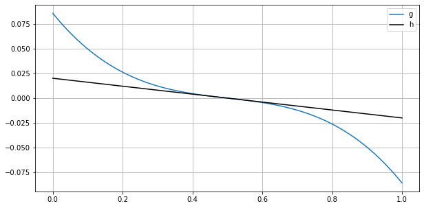
Figure 3: A linear lower bound for $|g|$, $k=3$ and $p=0.18$.

Let us define an auxiliary process $R^{*}_{n}$ by the stochastic recursion $R^{*}_{k}=1$ and for $n\geq k$

$$R^{*}_{n+1}=R^{*}_{n}+\frac{B_{n}\left(h(R^{*}_{n})+R^{*}_{n}\right)-R^{*}_{n}}{n+1}~{},$$

where $B_{n}\left(h(R^{*}_{n})+R^{*}_{n}\right)$ is a Bernoulli random variable with parameter $h(R^{*}_{n})+R^{*}_{n}$, conditionally independent of $R^{*}_{n}$. In particular,

$$\mathbb{E}\left[B_{n}\left(h(R^{*}_{n})+R^{*}_{n}\right)-R^{*}_{n}|R^{*}_{n}=t\right]=h(t)~{}.$$

Since the value of $g$ (for $(R_{n})$) and $h$ (for $(R^{*}_{n})$) represents a drift in the processes $R_{n}$ and $R^{*}_{n}$ we expect that the process $(R^{*}_{n})$ is further away from $1/2$. Indeed, we may introduce a coupling as follows. Define the stopping time $T^{*}$ as the first time $R^{*}$ reaches $1/2$:

$$T^{*}:=\min\left\{n\geq k:\ R^{*}_{n}\leq\frac{1}{2}\right\}~{}.$$

Since for the times $n\in[k,T^{*}]$, $h(R^{*}_{n})\geq g(R_{n})$, we may use a similar coupling argument as in Section 4.1. Thus, there is a coupling of $R^{*}$ and $R$ such that

$$\forall n\in[k,T^{*}];\ R_{n}\leq R^{*}_{n}~{}.$$

From this coupling, for $T$ defined in Lemma 2 we have

$$\mathbb{P}\left\{T=+\infty\right\}\leq\mathbb{P}\left\{T^{*}=+\infty\right\}~{}.$$ (4.5)

Observe that in the case of $k=1$, $g$ is linear and the two processes $R_{n}$ and $R^{*}_{n}$ coincide. The linear case was analyzed in Addario-Berry et al. [1] and we may use their results to understand the behavior of $R_{n}^{*}$. Indeed, the process defined in Addario-Berry et al. [1] is the same as $R^{*}$ if one sets the flip probability of Addario-Berry et al. [1] equal to $-g^{\prime}(1/2)/2$ and starts at time $k$. They prove that if $p\geq 1/4$, then, for the process starting at time $1$, majority voting has an error probability of $1/2+o(1/2)$. Lemma 2 implies that this process reaches $1/2$ in finite time almost surely. So even conditioned on its value being $1$ at time $k$ it will reach $1/2$ in finite time almost surely. This proves that even for $R_{n}^{*}$ starting at time $k$ its error probability is $1/2+o(1)$. According to Lemma 2 this implies that for this range of $p$, $\mathbb{P}\left\{T^{*}=+\infty\right\}=0$. Hence, using Lemma 2 and (4.5), shows that if $g^{\prime}(1/2)\leq-\frac{1}{2},$ then

$$\limsup_{n\to\infty}R^{maj}(n,p)=\frac{1}{2}~{}.$$

Lemma 3 shows that $\lim_{n\to\infty}R^{maj}(n,p)=1/2$. Because $g^{\prime}(1/2)=(1-2p)\alpha_{k}-1$, we just proved that if $p\geq 1/2-1/4\alpha_{k}$, then

$$\lim_{n\to\infty}R^{maj}(n,p)=\frac{1}{2}~{},$$

completing the proof of the third statement of Theorem 1.

4.2.2 Intermediate rate

It remains to study the “intermediate” case $p\in[1/2-1/(2\alpha_{k}),1/2-1/(4\alpha_{k}))$. To this end, we may couple $R_{n}$ to a process for which majority voting outperforms random guessing. Let us fix $p\in[1/2-1/(2\alpha_{k}),1/2-1/(4\alpha_{k}))$, which implies that $g^{\prime}(1/2)/2>-1/4$. Then choose $q=-g^{\prime}(1/2)/2+\epsilon$ with $\epsilon>0$ small enough so that $q<1/4$ and $g(0)>h(0)$. We define the linear function $h(t):=-2q(t-1/2)$, and as illustrated in Figure 4, we denote by $a$ and $b$ the intersection points between $h$ and $g$ (apart from $1/2$). More precisely $a$ and $b$ are defined as the the roots of $g-h$ distinct from $0$. Since $g-h$ is strictly convex on $(0,1/2)$ and $(g-h)(0)>0$, $(g-h)^{\prime}(1/2)<0$, $a$ and $b$ are well defined and sit respectively in $(0,1/2)$ and $(1/2,1)$.

Figure 4: Comparison of $h$ and $g$, for $k=3$ and $p=0.34$ (rescaled for clarity).

We define $R^{*}_{n}$ similarly as in the previous section but now with $h(t)=-2q(t-1/2)$, that is $R^{*}_{k}=1$ and

$$R^{*}_{n+1}=R^{*}_{n}+\frac{B_{n}\left(h(R^{*}_{n})+R^{*}_{n}\right)-R^{*}_{n}}{n+1}~{},$$

where the $B_{n}$ are conditionally independent Bernoulli random variables. In particular,

$$\mathbb{E}\left[B_{n}\left(h(R^{*}_{n})+R^{*}_{n}\right)-R^{*}_{n}|R^{*}_{n}=t\right]=-2q\left(t-\frac{1}{2}\right)~{}.$$

Just as in the previous section, we may use the analysis of Addario-Berry et al. [1] for the case $k=1$ with mutation probability of $q$. Addario-Berry et al. [1] state that for the process starting at time $1$ and for $q<1/4$ majority voting is better than random guessing. A simple coupling from the process starting at time $1$ and $R^{*}_{n}$ proves that this statement holds for $R_{n}^{*}$. Thus, from Lemma 2 it follows that

$$\mathbb{P}\left\{\forall n\geq k:\ R^{*}_{n}>\frac{1}{2}\right\}>0~{}.$$

Now, from Lemma 1 we deduce that both processes $R_{n}$ and $R^{*}_{n}$ converge almost surely to $1/2$ and exceed $b$ only finitely many times. Thus, there exists an almost surely finite random time $T^{\prime}$ such that and $\forall n\geq T^{\prime};$ $R_{n}\leq b$ and $R^{*}_{n}\leq b$. We use similar coupling arguments as in Section 4.1. So, on the event that $R^{*}$ does not reach $1/2$ we can couple $R_{n}$ and $R^{*}_{n}$ from $T^{\prime}$ onwards such that $R_{n}\geq R^{*}_{n}$. This proves that

$$\mathbb{P}\left\{\forall n\geq T^{\prime}:\ R_{n}>\frac{1}{2}\ |\ T^{\prime}\right\}>0~{}.$$

Using that $T^{\prime}$ is finite almost surely and Lemma 2 we conclude that majority voting is better than random guessing in this regime. More precisely, if $1/2-1/2\alpha_{k}\leq p<1/2-1/4\alpha_{k}$, then

$$\limsup_{n\to\infty}R^{maj}(n,p)<\frac{1}{2}~{}.$$

This completes the proof of Theorem 1.

5 A general lower bound

In this final section we derive a lower bound for the probability of error that holds for all mutation probabilities. In particular we show the following.

Proposition 1.

Let $k$ be a positive odd integer and let $k/2<\ell<k$. Assume that initially there are $\ell$ red vertices, that is $R_{k}=\ell/k$. Letting

$$h_{k}:=\mathbb{P}\left\{\text{Beta}\left(\frac{k+1}{2},\frac{k+1}{2}\right)\geq 1-\frac{1}{k}\right\}~{},$$

the probability of error of the majority rule satisfies

$$\inf_{0\leq p\leq 1\atop\ n\geq 2\ell}\mathbb{P}\left\{b_{n}^{maj}\neq b_{k}^{maj}\right\}\geq\frac{1}{2}h_{k}^{2\ell-k}~{}.$$

Proof.   The proposition follows by simply considering the event that the first $2\ell-k$ new vertices are all blue. In that case, at time $2\ell$ the number of red and blue vertices are equal. We may write, for any $n\geq 2\ell$,

$$\mathbb{P}\left\{b_{n}^{maj}\neq b_{k}^{maj}\right\} \geq\mathbb{P}\left\{b_{n}^{maj}\neq b_{k}^{maj}\ |\ c_{k+1}=\cdots=c_{2\ell}=B\right\}\times\mathbb{P}\left\{c_{k+1}=\cdots=c_{2\ell}=B\right\}~{}.$$

From the symmetry of our model, $\mathbb{P}\left\{b_{n}^{maj}\neq b_{k}^{maj}\ |\ c_{k+1}=\cdots=c_{2\ell}=B\right\}=1/2$. Thus

$$\mathbb{P}\left\{b_{n}^{maj}\neq b_{k}^{maj}\right\}\geq\frac{\mathbb{P}\left\{c_{k+1}\cdots c_{2\ell}=B\right\}}{2}~{}.$$

To estimate the probability on the right-hand side, we use (2.4), which implies

$$\mathbb{P}\left\{c_{i}=B\right\}=\int_{f(R_{i})}^{1}\left(x(1-x)\right)^{\frac{k-1}{2}}\frac{\Gamma(k+1)}{\Gamma^{2}\left(\frac{k+1}{2}\right)}dx~{}.$$

If $R_{k}=\ell/k$ and $c_{k+1}=\cdots=c_{i-1}=B$, where $k<i\leq 2k$, then $R_{i-1}=\ell/i$. Since $0\leq p\leq 1/2$,

$$f(R_{i-1})=(1-2p)\frac{\ell}{i}+p\leq\max\left(\frac{1}{2},\frac{\ell}{i}\right)\leq\frac{k-1}{k}=1-\frac{1}{k}~{}.$$

Therefore,

$$\min_{k<i\leq 2\ell}\mathbb{P}\left\{c_{i}=B\ \mid\ c_{k+1}=\cdots=c_{i-1}=B\right\}\geq h_{k}~{},$$

as claimed.  

6 Concluding remarks

In this paper we study the majority rule for guessing the initial bit values at the roots of a random recursive $k$-dag in a broadcasting model. The main result of the paper characterizes the values of the mutation probability for which the majority rule performs strictly better than random guessing. Even in this exact model, many interesting questions remain open. For example, we do not have sharp bounds for the probability of error. It would also be interesting to study other, more sophisticated, classification rules that take the structure of the observed $k$-dag into account. In particular, the optimal probability of error (as a function of $k$ and the mutation probability $p$) is far from being well understood. For an initial study of localizing the toot vertices, we refer the interested reader to Briend et al. [4].

References

- Addario-Berry et al. [2022] Louigi Addario-Berry, Luc Devroye, Gábor Lugosi, and Vasiliki Velona. Broadcasting on random recursive trees. The Annals of Applied Probability, 32(1):497–528, 2022.
- Bertoin [2022] Jean Bertoin. Limits of Pólya urns with innovations, 2022. URL https://arxiv.org/abs/2204.03470.
- Bhabak et al. [2014] Puspal Bhabak, Hovhannes A. Harutyunyan, and Shreelekha Tanna. Broadcasting in Harary-like graphs. In 2014 IEEE 17th International Conference on Computational Science and Engineering, pages 1269–1276, 2014.
- Briend et al. [2023, to appear] Simon Briend, Francisco Calvillo, and Gábor Lugosi. Archaeology of random recursive dags and Cooper-Frieze random networks. Combinatorics, Probability and Computing, 2023, to appear.
- Coolen et al. [2017] Ton Coolen, Alessia Annibale, and Ekaterina Roberts. Generating Random Networks and Graphs. Oxford University Press, 2017. ISBN 9780198709893.
- Crimaldi et al. [2022] Irene Crimaldi, Pierre-Yves Louis, and Ida G. Minelli. An urn model with random multiple drawing and random addition. Stochastic Processes and their Applications, 147:270–299, 2022.
- Desmarais et al. [2021] Colin Desmarais, Cecilia Holmgren, and Stephan Wagner. Broadcasting induced colourings of random recursive trees and preferential attachment trees. arXiv preprint arXiv:2110.15050, 2021.
- Evans et al. [2000] William Evans, Claire Kenyon, Yuval Peres, and Leonard J. Schulman. Broadcasting on trees and the Ising model. The Annals of Applied Probability, 10(2):410 – 433, 2000.
- Harutyunyan and Li [2020] Hovhannes A. Harutyunyan and Zhiyuan Li. A new construction of broadcast graphs. Discrete Applied Mathematics, 280:144–155, 2020.
- Janson [2004] Svante Janson. Functional limit theorems for multitype branching processes and generalized pólya urns. Stochastic Processes and their Applications, 110(2):177–245, 2004.
- Janson [2019] Svante Janson. Random replacements in Pólya urns with infinitely many colours. Electronic Communications in Probability, 24:1 – 11, 2019.
- Janson and Mossel [2004] Svante Janson and Elchanan Mossel. Robust reconstruction on trees is determined by the second eigenvalue. Annals of Probability, 32(3B):2630–2649, 2004.
- Knape and Neininger [2014] Margarete Knape and Ralph Neininger. Pólya urns via the contraction method. Combinatorics, Probability and Computing, 23(6):1148–1186, 2014.
- Kuba and Mahmoud [2017] Markus Kuba and Hosam M. Mahmoud. Two-color balanced affine urn models with multiple drawings. Advances in Applied Mathematics, 90:1–26, 2017.
- Makur et al. [2020] Anuran Makur, Elchanan Mossel, and Yury Polyanskiy. Broadcasting on random directed acyclic graphs. IEEE Transactions on Information Theory, 66(2):780–812, 2020.
- Mossel [2001] Elchanan Mossel. Reconstruction on trees: beating the second eigenvalue. The Annals of Applied Probability, 11(1):285–300, 2001.
- Mossel [2004] Elchanan Mossel. Survey: information flow on trees. In Graphs, morphisms and statistical physics, volume 63 of DIMACS Ser. Discrete Math. Theoret. Comput. Sci., pages 155–170. Amer. Math. Soc., Providence, RI, 2004.
- Pemantle [1990] Robin Pemantle. Nonconvergence to unstable points in urn models and stochastic approximations. The Annals of Probability, 18(2):698–712, 1990.
- Pemantle [2007] Robin Pemantle. A survey of random processes with reinforcement. Probability Surveys, 4:9–12, 2007.
- Sly [2011] Allan Sly. Reconstruction for the Potts model. The Annals of Probability, 39(4):1365 – 1406, 2011.
- Wei [1979] LJ Wei. The generalized Pólya’s urn design for sequential medical trials. The Annals of Statistics, 7(2):291–296, 1979.
- Zhang [2022] Li-Xin Zhang. Convergence of randomized urn models with irreducible and reducible replacement policy. arXiv preprint arXiv:2204.04810, 2022.