A New Galaxy Cluster Merger Capable of Probing Dark Matter: Abell 56

Abstract

We report the discovery of a binary galaxy cluster merger via a search of the redMaPPer optical cluster catalog, with a projected separation of 535 kpc between the BCGs. Archival XMM-Newton spectro-imaging reveals a gas peak between the BCGs, suggesting a recent pericenter passage. We conduct a galaxy redshift survey to quantify the line-of-sight velocity difference ($153\pm 281$ km/s) between the two subclusters. We present weak lensing mass maps from archival HST/ACS imaging, revealing masses of $M_{200}=4.5\pm 0.8\times 10^{14}$ and $2.8\pm 0.7\times 10^{14}$ M_⊙ associated with the southern and northern galaxy subclusters respectively. We also present deep GMRT 650 MHz data revealing extended emission, 420 kpc long, which may be an AGN tail but is potentially also a candidate radio relic. We draw from cosmological n-body simulations to find analog systems, which imply that this system is observed fairly soon (60-271 Myr) after pericenter, and that the subcluster separation vector is within 22^∘ of the plane of the sky, making it suitable for an estimate of the dark matter scattering cross section. We find $\frac{\sigma_{\rm DM}}{m}=1.1\pm 0.6$ cm²/g, suggesting that further study of this system could support interestingly tight constraints.

1 Introduction

A collision of two galaxy clusters dramatically reveals the contrasting behaviors of gas, galaxies, and dark matter (DM). Seminal papers on the Bullet Cluster provided a “direct empirical proof of dark matter” (Clowe et al., 2006) as well as limits on the scattering cross-section of DM particles with each other (Markevitch et al., 2004; Randall et al., 2008), aka DM “self-interaction.” The Bullet constraint, $\frac{\sigma_{\rm DM}}{m}<0.7$ cm²/g, is still quite large in particle physics terms—roughly at the level of neutron-neutron scattering. In principle, ensembles of merging clusters enable tighter constraints (Harvey et al., 2015; Wittman et al., 2018b) but these are complicated by the fact that few systems have well-modeled dynamics. Specifically, the time since pericenter, pericenter speed, and viewing angle cannot be extracted from systems that have more than two merging subclusters. Even with binary mergers, other factors may hinder the study of dark matter, such as a merger axis closer to the line of sight rather than the plane of the sky or bright stars that limit deep optical observations. Hence there is interest in finding more “clean” binary systems with merger axis close to the plane of the sky.

   

Figure 1: Abell 56: 0.4-1.25 keV XMM-Newton contours over SDSS multiband (left) and HST/ACS F814W (right) images.

Historically, merging systems were discovered upon notice of disturbed X-ray morphology, which typically happened serendipitously in pointed observations. Meanwhile, modern optical sky surveys find tens of thousands of clusters and promise to find many more as they get wider and deeper (Racca et al., 2016; Ivezić et al., 2019). These surveys potentially contain new binary mergers, if appropriate cuts can filter out tens of thousands of more ordinary clusters. We have developed a new selection method based on the redMaPPer (Rykoff et al., 2014) cluster catalog, which is in turn based on the ${\sim}$10,000 deg² Sloan Digital Sky Survey (SDSS; York et al., 2000) imaging. We select clusters not dominated by a single brightest cluster galaxy (BCG), in which there is substantial angular separation between the top BCG candidates. These clusters become candidate mergers, which are then checked against archival XMM-Newton and Chandra data where available; if the X-ray peak is between the BCGs, the candidate is worthy of additional followup. Because these two X-ray archives consist of pointed observations rather than a uniform survey, our initial candidates do not form a sample with well-defined selection criteria. Nevertheless, a few initial candidates are worthy of immediate study in their own right. In this paper we present the first such candidate, RM J003353.1-075210.4, which we identify as Abell 56 as explained in §2. Additional sections in this paper present a galaxy redshift survey of the system (§3); a weak lensing analysis (§(1)); a search for analog systems in a cosmological simulation (§5); radio observations in search of a radio relic that could outline a merger shock (§6); and a constraint on the dark matter scattering cross section $\frac{\sigma_{\rm DM}}{m}$(§7). We assume a flat $\Lambda$CDM cosmology with $H_{0}=69.6$ km/s and $\Omega_{m}=0.286$.

2 Abell 56: initial overview

Nomenclature. The redMaPPer designation for this cluster is RM J003353.1-075210.4. The original coordinates for Abell 56 (Abell et al., 1989 ; hereafter ACO) are nearly $5^{\prime}$ north of the redMaPPer position. Although ACO cite the positional uncertainty as $2.5^{\prime}$, inspection of the SDSS imaging reveals no other clusters in the area, suggesting that the ACO coordinates are off by more than their nominal uncertainty. (The limited depth of the ACO catalog is such that any real ACO cluster must be in the redMaPPer catalog.) Indeed, the widely-used SIMBAD database resolves the name “Abell 56” to the redMaPPer position, as does the SDSS Navigator noted above. Hence we identify this cluster as Abell 56. Note, however, that the NASA/IPAC Extragalactic Database (NASA/IPAC Extragalactic Database (2019), NED) resolves this name to the original ACO coordinates.

This cluster has also been detected by the Planck Sunyaev-Zel’dovich survey (Planck Collaboration et al., 2016), with the designation PSZ2 G109.99-70.28. This gas peak position is $1.3^{\prime}\pm 2.4^{\prime}$ from the redMaPPer position and $4.0^{\prime}\pm 2.4^{\prime}$ from the ACO position. Hence Planck Collaboration et al. (2016) adopted the redMaPPer position while adopting “ACO 56” as the identifier in their union catalog. As a result, a search for G109.99-70.28 on SIMBAD yields the redMaPPer position; however NED yields the much more uncertain gas peak position.

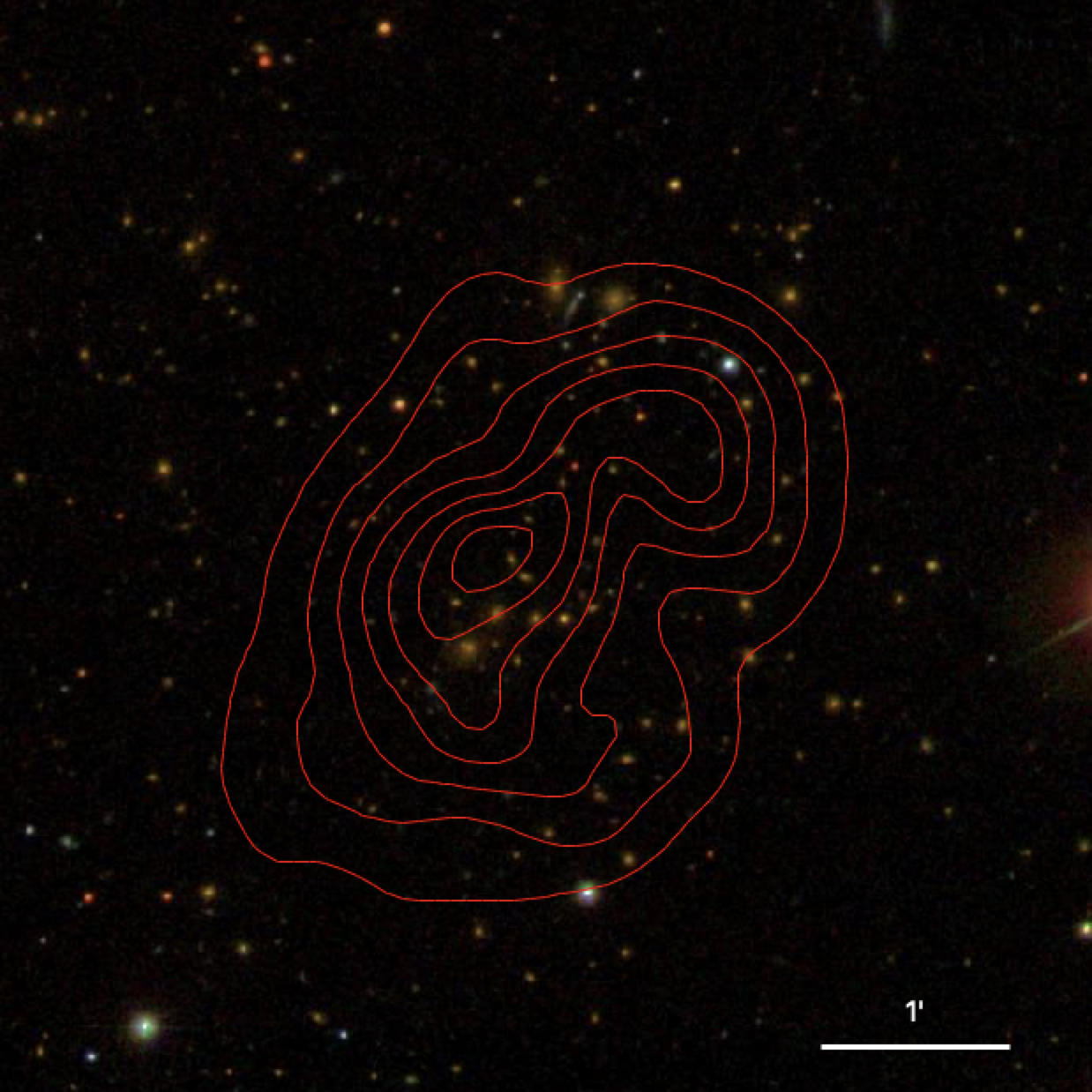
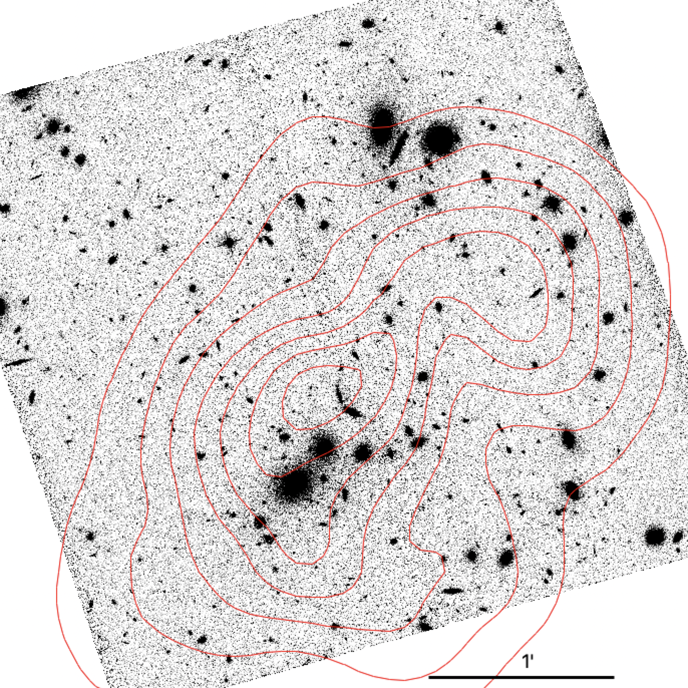
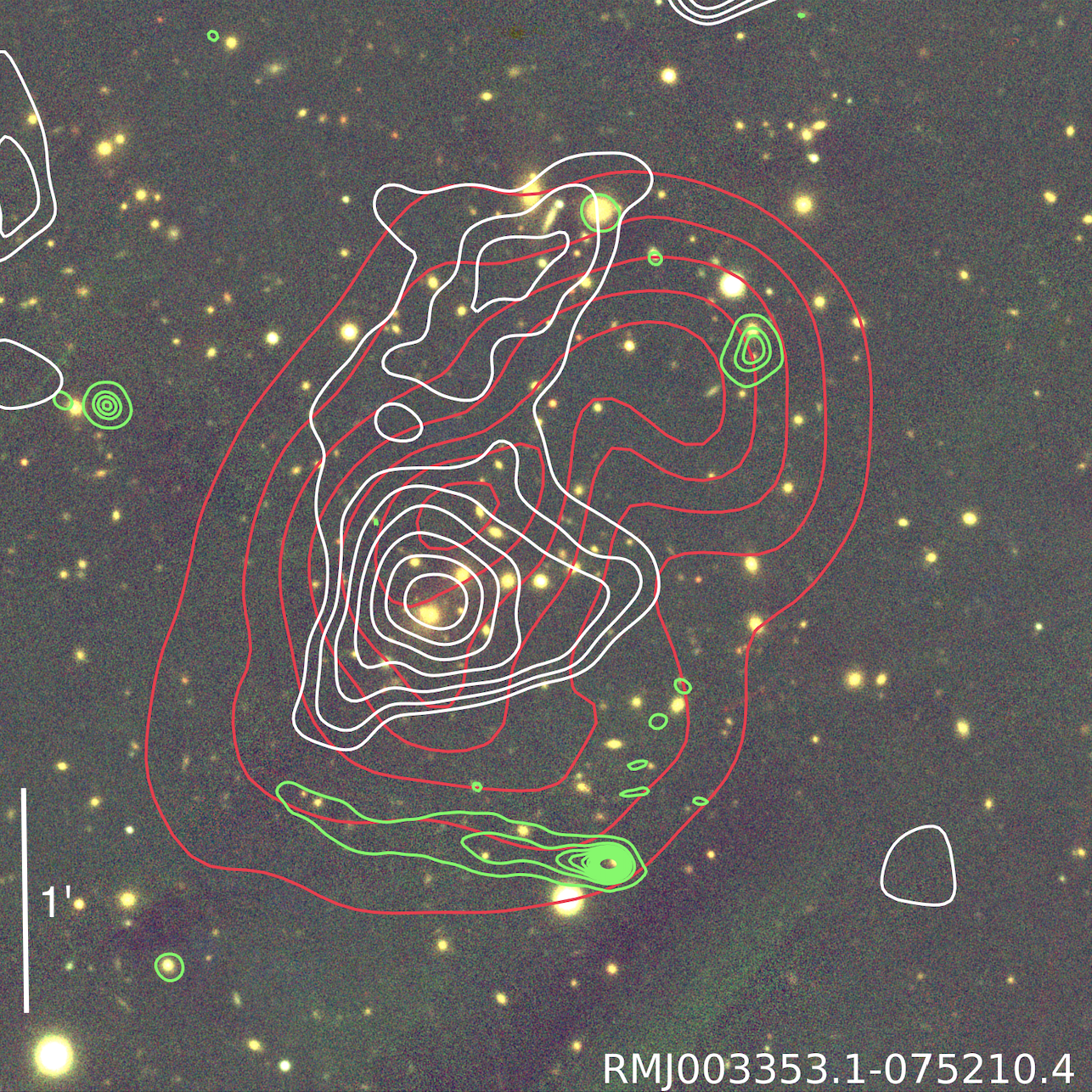
BCGs and redshifts. Figure 1 presents two views of Abell 56: with XMM-Newton contours (see below) over SDSS multiband imaging and over a single-band (F814W) archival image from the Hubble Space Telescope Advanced Camera for Surveys (HST/ACS) (see §(1)). At the redMaPPer photometric redshift of 0.30, the physical scale is 4.5 kpc/arcsec. There are two galaxy subclusters separated by close to $2^{\prime}$ (530 kpc), with the X-ray peak located along the subcluster separation vector, about $32^{\prime\prime}$ (140 kpc) from the southern subcluster. These numbers will be refined with further data in later sections of this work.

The southern subcluster is dominated by a galaxy observed by the Baryon Oscillation Spectroscopic Survey (BOSS; Dawson et al., 2013) to be at $z=0.30231$; redMaPPer assigns this galaxy 84% probability of being the overall BCG. The northern subcluster has two galaxies that appear nearly equally salient in Figure 1; the eastern one (about 0.2 mag brighter) is assigned 16% probability of being the overall BCG and BOSS places it at $z=0.30475$. redMaPPer technically assigns some nonzero BCG probability to the second-brightest galaxy in each subcluster, but in each case it is only $0.017\%$, which we consider negligible.

Repp & Ebeling (2018) briefly considered this cluster as part of an 86-cluster sample. It is classified in their Table 6 as being in the most disturbed of their four optical morphology classes.

Merger basics. Taking the BCGs as tracers for a first calculation of the merger geometry, we find a projected separation of 118^′′ (535 kpc) and a line-of-sight velocity difference of 565 km/s. For comparison, the projected separation in the X-ray selected Bullet cluster is 720 kpc (Bradač et al., 2006; Clowe et al., 2006) and those in Golovich et al. (2019) radio-selected sample of merging clusters are generally closer to 1 Mpc, indicating that more time since pericenter (TSP) has passed. This suggests the potential of optical selection to find systems with smaller separations hence less TSP. Because a complete understanding of the merging process will require snapshots of systems spanning a range of TSP, optical selection may find its place within a range of complementary selection methods.

Richness and related estimates. Rykoff et al. (2014) give the optical richness $\lambda$ (a measure of how many galaxies are in the cluster, within a certain luminosity range below the BCG) as 128. Simet et al. (2017) calibrated the relation between weak lensing mass and $\lambda$ (including its scatter), from which we estimate the mass of Abell 56 to be $M_{200}=10.4^{+7.6}_{-4.6}\times 10^{14}\ h^{-1}$ M_⊙. Sereno & Ettori (2017) implemented a system for mass forecasting with proxies, taking into account various biases, and found $M_{200}=11.49\pm 0.89\times 10^{14}$ M_⊙ for this system based on its redMapper richness. They also found $M_{500}=7.09\pm 0.77\times 10^{14}$ M_⊙ using $Y_{\rm 500}$, a measure of the Sunyaev-Zel’dovich effect, as a proxy. For comparison, Planck Collaboration et al. (2016) found $M_{500}=5.62^{+0.54}_{-0.58}\times 10^{14}$ M_⊙ from their scaling relation based on the same $Y_{\rm 500}$ measurement.

From the scaling relations of Rozo & Rykoff (2014) one would expect the X-ray temperature $T_{X}$ to be around 7 keV with up to 40% scatter at fixed richness. Because this is a merging cluster, the X-ray properties may vary from the scaling relations even more than usual.

X-ray properties from archival data. The cluster was observed with the XMM-Newton European Photon Imaging Camera (EPIC) in 2010 (Obs.ID 0650380401, P.I. Allen). The exposure times were 7121 s, 7127 s, and 5533 s for the MOS1, MOS2, and PN instruments, respectively. As the short exposure does not allow for a detailed analysis of the intracluster medium (ICM) properties and the cluster morphology, we restricted our analysis to obtaining a point-source-subtracted, exposure-corrected image, as well as a global temperature and luminosity for the cluster.

We performed the data reduction using the XMM-Newton Science Analysis System (SAS) version 19.0.0. We excluded periods of high soft-proton background by imposing a cutoff of 0.4 (0.8) on the soft-proton rate for the MOS (PN) detectors, which resulted in filtered exposure times of 6817 s, 6621 s, and 4178 s for MOS1, MOS2, and PN, respectively. Only single-to-quadruple events from MOS and single-to-double events from PN were used in our analysis. Point-source detection and masking were performed by the cheese routine from the ESAS package. The contours in Figure 1 are from the 0.4-1.25 keV band after point-source masking and exposure correction, using the procedure described in the XMM ESAS Cookbook (Snowden & Kuntz, 2014) and adaptively smoothed using the adapt routine from ESAS.

In order to obtain a background-subtracted spectrum, we used the double-subtraction method described in Arnaud et al. (2002). We defined the source region as a circle with a 90^′′ radius centered on the cluster, whereas the background was extracted from a slightly larger circular region away from the cluster. Blank-sky files (Carter & Read, 2007) were used to mitigate the effects of the spatial variation of background components across the detector. For a detailed description of the method, we refer to Arnaud et al. (2002). Using XSPEC (Arnaud, 1996), we fit the spectrum to an apec model, multiplied by a phabs model to account for galactic absorption. We obtained a total unabsorbed luminosity in the $0.5-10.0$ keV range of $L_{X}=3.8\pm 0.2\times 10^{44}$ erg/s and a temperature $T_{X}=5.9^{+1.1}_{-0.8}$ keV, where the uncertainties represent the $90\%$ confidence intervals.

3 Redshift survey and clustering kinematics

3.1 Redshift survey

Observational setup. We observed Abell 56 with the DEIMOS multi-object spectrograph (Faber et al., 2003) at the W. M. Keck Observatory on July 1, 2022 (UT). The DEIMOS field of view is approximately 16${}^{\prime}\times 4^{\prime}$, making it well suited to merging clusters when the long axis is placed along the subcluster separation vector. We prepared two slitmasks with approximately sixty 1^′′ wide slits in each. Galaxies were selected for targeting based on (i) a preference for brighter targets; and (ii) a preference for galaxies likely to be in the cluster based on Pan-STARRS photometric redshifts (Beck et al., 2021). Because the photometric redshifts are imprecise, this approach naturally helps probe for potential foreground/background structures that could affect the modeling of Abell 56. Specifically, each Pan-STARRS photometric redshift $z_{\rm PS}$ has a corresponding uncertainty $\sigma_{\rm PS}$ such that the likelihood of the galaxy being in a cluster at redshift $z_{\rm cl}$ is

$$\mathcal{L}\propto\frac{1}{\sigma_{\rm PS}}\exp\frac{(z_{\rm PS}-z_{\rm cl})^{2}}{2\sigma_{\rm PS}^{2}}$$ (1)

The median value of $\sigma_{\rm PS}$ was 0.16, so a broad range of redshifts was included. We then upweighted brighter galaxies by applying a multiplicative weight $(24-r)$, where $r$ is the apparent $r$ magnitude, to quantify the priority of each galaxy as input to the slitmask design software dsimulator; larger numbers indicate higher priority. We manually raised the priority of a few galaxies that potentially formed a foreground group at the north end of the field.

We used the 1200 line mm^-1 grating, which results in a pixel scale of 0.33 Å pixel^-1 and a resolution of ${\sim}1$ Å (50 km/s in the observed frame). The grating was tilted to observe the wavelength range $\approx$ 4200–6900 Å(the precise range depends on the slit position), which at $z\approx 0.3$ includes spectral features from the [OII] 3727 Å doublet to the magnesium line at 5177 Å. The total exposure time was 45 (77) minutes on the first (second) mask, divided in three (four) exposures. The seeing was roughly 1″, with minor variations over time.

Data reduction and redshift extraction. We calibrated and reduced the data to a series of 1-D spectra using PypeIt (Prochaska et al., 2020, 2020). We double-checked the arc lamp wavelength calibration against sky emission lines, and found good agreement.

To extract redshifts from the 1-D spectra we wrote custom Python software to emulate major elements of the approach used by the DEEP2 (Newman et al., 2013) survey using the same instrument. The throughput as a function of wavelength varies from slit to slit, hindering direct comparison to template spectra. Because throughput is generally a slowly varying function of wavelength, the spectra are compared to templates only after removing the slowly varying trends from each. First, telluric absorption features are reversed using Mauna Kea models from the PypeIt development suite. Next, we create a smooth model or unsharp mask by convolving the 1-D spectrum with a kernel 150 Å wide, which is uniform but for a 10 Å diameter hole in the center. Finally, the intensity of each pixel in the 1-D spectrum is expressed as a fraction of the intensity in the smooth model.

The same operations are performed on redshifted versions of the galaxy templates from the Sloan Digital Sky Survey, and a $\chi^{2}$ value is computed for each template-redshift combination. A user then inspects the match between the data and the model with the global minimum $\chi^{2}$, or other models at local minima, before determining whether a redshift is secure. A secure redshift may not appear at the global minimum due to poorly subtracted sky lines or other artifacts (e.g., a spurious “line” with spuriously small uncertainties may appear at the gap between CCDs). Furthermore, some slits suffer from vignetting at the red end, which appears as a drop in intensity too steep to be removed by the unsharp masking process. In these cases the user specifies a maximum wavelength to consider for template matching. A negligible fraction of slits contained stars, so we did not include stellar templates in the automated search; users can manually classify a spectrum as a star without extracting a redshift.

The uncertainty in the redshift is initially computed from the curvature of the $\chi^{2}$ surface about the minimum, and is typically $\lesssim 10^{-4}$ (23 km/s in the frame of the cluster). We compared redshifts obtained by different users on different computing hardware, operating systems, and Python installations. We found that user-dependent uncertainty is also $\lesssim 10^{-4}$, mostly due to specification of the maximum wavelength. We therefore add $10^{-4}$ in quadrature to the uncertainty derived from the curvature of the $\chi^{2}$ surface to derive a final uncertainty estimate. We found 54 and 48 secure redshifts in the two masks respectively, for a total of 102. These are listed in Table 3.1.

Table 1: Galaxy redshifts

RA (deg)	DEC (deg)	z	uncertainty
8.410133	-7.758144	0.370305	0.000107
8.412567	-7.747167	0.370005	0.000102
8.411033	-7.742000	0.370055	0.000103
8.412454	-7.750711	0.411192	0.000182
8.414025	-7.767139	0.361506	0.000100
8.418721	-7.738369	0.124575	0.000103
8.419221	-7.752617	0.309164	0.000132
8.424929	-7.768175	0.550809	0.000390
8.439262	-7.728628	0.342070	0.000149
8.449196	-7.770197	0.300759	0.000103
8.451654	-7.772564	0.301399	0.000100
8.483425	-7.776081	0.305369	0.000106
8.430800	-7.878178	0.285649	0.000108
8.433154	-7.865233	0.302410	0.000111
8.436871	-7.800781	0.303911	0.000101
8.437129	-7.820883	0.307063	0.000103
8.439008	-7.874475	0.310816	0.000104
8.442646	-7.833144	0.295355	0.000102
8.442646	-7.833144	0.304912	0.000273
8.442892	-7.838442	0.296056	0.000101
8.443604	-7.795317	0.368704	0.000100
8.446533	-7.918775	0.510949	0.000554
8.446804	-7.847947	0.302537	0.000120
8.446900	-7.865711	0.292854	0.000103
8.448988	-7.939147	0.301960	0.000111
8.451133	-7.910875	0.305312	0.000107
8.448746	-7.942206	0.764905	0.000207
8.452063	-7.952244	0.364001	0.000107
8.455208	-7.976750	0.306263	0.000109
8.454325	-7.842231	0.291603	0.000101
8.457279	-7.888228	0.309365	0.000103
8.457279	-7.888228	0.309039	0.000103
8.457421	-7.879375	0.300609	0.000104
8.460504	-7.866011	0.304762	0.000103
8.460571	-7.821856	0.312767	0.000104
8.462892	-7.842867	0.299458	0.000100
8.463775	-7.837614	0.304938	0.000101
8.463446	-7.852147	0.312048	0.000101
8.465396	-7.800806	0.209615	0.000103
8.466696	-7.805417	0.166386	0.000104
8.466279	-7.910831	0.300395	0.000119
8.466696	-7.805417	0.303377	0.000103
8.468108	-7.882522	0.301556	0.000102
8.469058	-7.866528	0.308831	0.000108
8.469108	-7.846475	0.300255	0.000108
8.470600	-7.894619	0.300445	0.000115
8.469867	-7.922953	0.299295	0.000100
8.472408	-7.810456	0.368080	0.000101
8.479588	-7.966142	0.301866	0.000104
8.487733	-7.926608	0.301159	0.000101
8.491658	-7.896106	0.297784	0.000100
8.494708	-7.913458	0.307990	0.000874
8.497242	-7.883722	0.298694	0.000107
8.512950	-7.938439	0.533748	0.000110
8.440079	-7.972850	0.304762	0.000106
8.438658	-7.847369	0.302260	0.000147
8.440954	-7.950100	0.761086	0.000358
8.441692	-7.832436	0.295155	0.000102
8.441692	-7.832436	0.304628	0.000120
8.444413	-7.918158	0.301403	0.000102
8.444925	-7.742297	0.298120	0.000119
8.445521	-7.845039	0.643521	0.000100
8.446550	-7.870319	0.303561	0.000101
8.443504	-7.981761	0.390419	0.000106
8.449642	-7.842747	0.371022	0.000101
8.448617	-7.785400	0.306663	0.000103
8.453133	-7.920878	0.293771	0.000101
8.455708	-7.876181	0.412010	0.000107
8.458538	-7.838819	0.316319	0.000101
8.458929	-7.864583	0.303911	0.000103
8.460292	-7.783261	0.263697	0.000101
8.459621	-7.840900	0.295088	0.000100
8.467704	-7.995767	0.449141	0.000103
8.463604	-7.836289	0.304228	0.000104
8.464392	-7.744386	0.127610	0.000100
8.464413	-7.885931	0.298040	0.000102
8.466088	-7.898686	0.299508	0.000104
8.465567	-7.866972	0.302907	0.000101
8.467179	-7.830192	0.302136	0.000114
8.470292	-7.732906	0.457597	0.000110
8.467813	-7.806775	0.166486	0.000103
8.471492	-7.765292	0.458958	0.000101
8.471050	-7.773569	0.276543	0.000101
8.474892	-7.873158	0.307967	0.000100
8.476692	-7.907672	0.368621	0.000100
8.477433	-7.955953	0.369154	0.000103
8.480146	-7.883764	0.296739	0.000107
8.478713	-7.778783	0.305796	0.000104
8.481079	-7.796372	0.370439	0.000102
8.481037	-7.852150	0.303194	0.000102
8.479967	-7.927103	0.292623	0.000104
8.484304	-7.771003	0.469204	0.000102
8.485038	-7.902189	0.412787	0.000105
8.486742	-7.826083	0.369608	0.000111
8.487963	-7.821725	0.367643	0.000108
8.487963	-7.821725	0.367550	0.000115
8.488279	-7.849608	0.304134	0.000101
8.490088	-7.816639	0.302260	0.000101
8.494679	-7.892922	0.144521	0.000101
8.497133	-7.756675	0.290352	0.000108
8.500467	-7.915733	0.458747	0.000103
8.503554	-7.811536	0.371723	0.000105

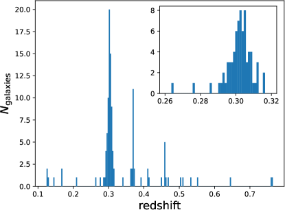
Comparison to archival redshifts. We searched NED for archival spectroscopic redshifts within a radius of 5^′, and found 16 galaxies, largely from BOSS (Dawson et al., 2013). Of these, five were galaxies that we had targeted. The mean redshift difference between independent measurements of the same target is $9$ km/s, with an rms scatter of $9$ km/s. We then removed the duplicates and merged the catalogs from NED and from our two masks to produce a final catalog of 113 galaxies. Figure 2 shows a histogram of these redshifts.

Figure 2: Redshift histogram, with inset showing the redshift interval around Abell 56.

3.2 Subclustering and kinematics

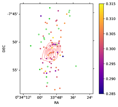
Non-Abell 56 structures. Figure 2 reveals a potential background cluster at $z=0.37$, and possibly another at $z=0.46$. To assess how strongly clustered these galaxies are on the sky, Figure 3 shows a sky map color-coded by redshift. Galaxies in the putative cluster at $z=0.37$ (0.46) are shown as open (closed) green circles, while galaxies near $z=0.30$ (i.e., associated with Abell 56) are shown with a continuous color map that contains no green. Neither set of background galaxies shows signs of clustering in space. Furthermore, we estimate the velocity dispersion of each set using the biweight estimator (Beers et al., 1990) and find only $279\pm 45$ ($105\pm 48$) for the structure at $z=0.37$ (0.46). Uncertainties on biweight estimators are obtained by the jackknife method throughout this paper. These velocity dispersions are far less than the velocity dispersion of Abell 56 (below), suggesting that they are an order of magnitude less massive and unlikely to substantially contaminate the weak-lensing and X-ray maps presented below.

Figure 3: Redshift map. Abell 56 galaxies are coded with a continuous color map, while galaxies in the putative background cluster at $z=0.37$ (0.46) are shown as open (closed) green circles. XMM-Newton contours are shown in red.

Abell 56. Of 67 galaxies in the $0.285\leq z\leq 0.314$ window, the biweight estimate for the systemic redshift is $0.30256\pm 0.00058$. At this redshift, the physical scale is 4.521 kpc/arcsec given our adopted cosmological model (Wright, 2006). The redshift distribution is compatibile with a single Gaussian, according to a Kolmogorov-Smirnov test. This is consistent with the low line-of-sight velocity component $\Delta v_{\rm los}$ suggested by the archival redshifts of the north and south BCGs. The biweight estimate of velocity dispersion is $1264\pm 145$ km/s—rather large, but likely to be inflated by merger activity as noted below.

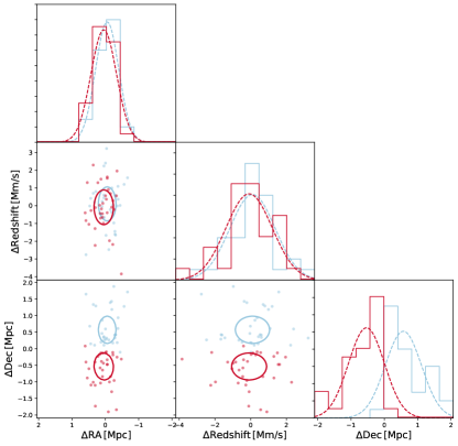
We use the mc3gmm code (Golovich et al., 2019) to assign galaxy membership to subclusters. This code models the distribution of galaxies in (RA, Dec, z) space as a mixture of $N$ elliptical Gaussian profiles (i.e., subclusters), with physically motivated priors on subcluster variance in each dimension as well as covariance (i.e., ellipticity and rotation). $N$ is determined by the user; we set $N{=}2$ based on the optical imaging and further supported by the lensing data presented in §(1). The user sets nonoverlapping bounds for the central (RA, Dec, z) of each subcluster to avoid degeneracies; mc3gmm maximizes the likelihood by adjusting the parameters within those bounds. We run mc3gmm on the galaxies in the redshift window $0.285\leq z\leq 0.314$ and the result is shown in Figure 4. The velocities of the subclusters are nearly identical, suggesting that the relative motion of the subclusters is in a direction close to the plane of the sky. The biweight estimate for the systemic redshift of the 33 (34) north (south) members is $0.30298\pm 0.00099$ ($0.30231\pm 0.00071$). This yields $\Delta v_{\rm los}=153\pm 281$ km/s.

The biweight velocity dispersion is $1283\pm 236$ km/s for the north subcluster, and $1251\pm 191$ for the south. Simulations of merging clusters (e.g., Pinkney et al., 1996; Takizawa et al., 2010) show that a pericenter passage in the plane of the sky boosts the observed velocity dispersion by a factor of ${\approx}1.5$ for hundreds of Myr afterward. Hence, one should not interpret these large velocity dispersions as indicative of extremely massive clusters.

Figure 4: Corner plot showing distribution of subcluster members in RA, DEC, and velocity space relative to the overall mean. Members of the north (south) subcluster are shown in blue (red).

4 Weak lensing analysis

We perform a weak-lensing analysis on the HST F814W imaging. Galaxies are detected in the F814W image with SExtractor (Bertin & Arnouts, 1996). For each galaxy, PSF models are generated following the method of Jee et al. (2007) by utilizing their publicly available PSF catalog. Each galaxy is fit with a PSF-convolved Gaussian distribution and the complex ellipticities are recorded (our ACS weak-lensing pipeline is outlined in Finner et al., 2017, 2021, 2023). Objects with ellipticity greater than 0.8, ellipticity uncertainty greater than 0.3, and intrinsic size (pre-psf) less than 0.5 pixels are removed to prevent spurious sources such as diffraction spikes around bright stars and poorly fit objects from entering the source catalog.

The next step is to eliminate as many foreground and cluster galaxies as possible, while still retaining a sizeable sample of background sources. With only single-band imaging available, we select galaxies with F814W AB magnitudes fainter than 24. We apply this magnitude cut to the GOODS-S photometric redshift catalog (Dahlen et al., 2013) and find that the contamination by foreground galaxies is expected to be $\sim 2\%$. Cluster galaxies may contribute additionally to the contamination. As their contamination should be radially dependent, we test the radial dependence of the source density. We find it to be flat, which suggests cluster galaxies are not significantly contaminating our source catalog. The final source catalog contains $\sim 43$ galaxies arcmin^-2. The source catalog is then provided to the FIATMAP code (Wittman et al., 2006) to create a surface mass density map. FIATMAP convolves the observed shear field with a kernel of the form r^-2 (1-exp(-r^2 2ri2)) exp(-r^2 2ro2) where $r_{i}$ and $r_{o}$ are inner and outer cutoffs, respectively. The inner cutoff is necessary to prevent amplification of shape noise in sources at small $r$, and was set to 50 arcsec. The outer cutoff suppresses noise that may come from unrelated structures along the line of sight at large projected separations, and is of limited value in a small field; we set it to 100 arcsec, which is comparable to the radius of the field. The results were pixelized onto a map with 1.5 arcsec pixels. In addition to this fiducial map, a family of viable reconstructions can be made by bootstrap resampling the shear catalog (see below). Figure 5 shows the fiducial map as a set of contours overlaid on a Pan-STARRS multiband image (Waters et al., 2020). Two weak lensing peaks are evident, associated with (albeit slightly offset from) each galaxy subcluster, with the X-ray peak in between. This confirms the basic merger scenario developed above.

Figure 5: Surface mass density contours from weak lensing (white) overlaid on a Pan-STARRS multiband image and red XMM-Newton surface brightness contours. The small closed contour between the subclusters is a trough. Green GMRT 650 MHz contours (§6) start at 70 $\mu$Jy/beam with increments of 680 $\mu$Jy/beam and a 4^′′ beam.

We estimate the mass of each subcluster by fitting a two-halo NFW model with a fixed mass-concentration relation from Diemer & Joyce (2019). To achieve the best-fit model, the shear of the two-halo model is derived at the position of each background galaxy and the chi-square is minimized. The effective distance ratio of the sources is set by the effective distance ratio of GOODS-S sources fainter than 24th magnitude. The best-fit two-halo model has a mass of $M_{200}=4.5\pm 0.8\times 10^{14}$ M_⊙ and $M_{200}=2.8\pm 0.7\times 10^{14}$ M_⊙ for the south and north subclusters, respectively. We allow the centroid of each halo to be fit and they converge to the projected mass distribution peaks. On the other hand, if we fix the halo centroids to the BCGs, we find the south and north subcluster masses decrease by $10\%$ and $60\%$, respectively. To test the dependence of the mass estimate on our choice of magnitude cut, we vary the magnitude constraint on the background catalog from 22nd to 25th magnitude and find that the mass estimates decrease for brighter magnitude cuts but within the mass uncertainty. To estimate the total mass of the cluster, we simulate two NFW halos at the projected separation of the two mass peaks. Integrating the model from the center of mass to $R_{200}$, we estimate the total mass of the cluster to be $M_{200}=9.7\pm 2.0\times 10^{14}$ M_⊙ ($M_{500}=7.1\pm 1.6\times 10^{14}$ M_⊙).

To further quantify the detection significance, we bootstrap resampled the source catalog to generate 1000 realizations of the mass map. As expected, the mean map yielded by these resamplings matches the fiducial map yielded by the original catalog. At any given sky position, we can measure the rms variation of surface mass density across the map realizations to obtain a noise map. The ratio of the fiducial map to this noise map is then a significance map. The peak of the southern (northern) subcluster is detected at a significance of $6.3$ ($5.5$).

The projected separation between the mass peaks, $d_{\rm proj}=438$ kpc, is important for the dynamical modeling in §5. To estimate the uncertainty on the peak locations, the peak from each of the 1000 realizations was recorded. The 1000 peaks were then passed to a $k$-means algorithm with the number of distributions fixed to two. The $k$-means algorithm iteratively calculates the centroid of the peaks and assigns peaks to each centroid until the centroid converges. This procedure yields two distributions of mass-peak locations, which are then processed with a kernel density estimator to find the $1\sigma$ and $2\sigma$ uncertainties. We find that the southern mass peak is consistent with its BCG at the $1\sigma$ level. In contrast, the northern mass peak is offset $19.2\pm 4.9$ arcsec ($87\pm 22$ kpc) to the south of the northern BCG. We address this offset further in §7. Our immediate goal here is to define a 68% confidence interval on the projected separation between mass peaks, which we find to be $96.9\pm 45.6$ arcsec ($438\pm 206$ kpc).

To further check the halo position uncertainties, we consider again the two-halo fit. As a model-driven procedure, this should be more robust against edge effects than the mapping procedure, which convolves the observed shear field. Nevertheless, as noted above, the halo center parameters converge to the projected mass distribution peaks. The positional uncertainties from the two-halo fit are smaller than those from the resampled mapping method. Hence our adoption of the values from the latter method is the more cautious approach.

5 Simulated analogs and dynamical parameters

We find analog systems in the Big Multidark Planck (BigMDPL) Simulation (Klypin et al., 2016) using the method of Wittman et al. (2018a) and Wittman (2019). The observables used to constrain the likelihood of any given analog and viewing angle are:

• the projected separation between mass peaks $d_{\rm proj}$, for which we use $438\pm 206$ kpc from §(1).

• the line-of-sight relative velocity $\Delta v_{\rm los}$, for which we use $153\pm 281$ km/s from §3.

• the subcluster masses, for which we use $M_{200}=4.5\pm 0.8\times 10^{14}$ M_⊙ and $M_{200}=2.8\pm 0.7\times 10^{14}$ M_⊙ for the south and north subclusters, respectively, from §(1). Note that dynamical timescales and velocities depend only weakly on the masses.

Table 2 lists the resulting highest probability density confidence intervals for time since pericenter (TSP), pericenter speed $v_{\rm max}$, viewing angle $\theta$ (defined as the angle between the subcluster separation vector and the line of sight, i.e. 90^∘ when the separation vector is in the plane of the sky), and the angle $\varphi$ between the current separation and velocity vectors. $\varphi$ is potentially an indicator of how head-on the trajectory is, as well as of merger phase (surpassing 90^∘ at apocenter). The likelihood ratio of analogs in the outbound vs. returning phase is 19:1. Table 2 also lists the confidence intervals for the dynamical parameters when the analysis is restricted to the outbound scenario. These particular parameters are not sensitive to the current merger phase.

Table 2: Dynamical parameters from analogs

Scenario	TSP (Myr)	$v_{\rm max}$ (km/s)	$\theta$ (deg)	$\varphi$ (deg)
68% CI
All	60-271	1960-2274	68-90	6-33
Outbound	90-291	1952-2282	68-90	0-26
95% CI
All	0-451	1729-2510	42-90	0-86
Outbound	0-366	1681-2489	44-90	1-67

6 Radio observations and results

Pericenter speeds in cluster mergers are typically greater than the sound speed in the gaseous ICM, so each subcluster launches a shock in the ICM of the other subcluster (Ha et al., 2018). In hydrodynamic simulations of the Bullet (Springel & Farrar, 2007) the shock begins at pericenter speed and loses very little speed over time, while the corresponding subcluster falls behind due to the gravity of the other subcluster. Our Abell 56 analogs do not include gas, but we use the pericenter speed, gravitational subcluster slowing, and analog time of observation to predict the separation between a subcluster and a hypothetical constant-velocity shock. We find ${\sim}200$ kpc separation in the outbound phase. The analogs indicate that an additional ${\approx}1.2$ Gyr passes before the subclusters return to the same projected separation en route to a second pericenter. In this time, a hypothetical constant-velocity shock would have proceeded over 2 Mpc further out. Therefore, observing the shock location could further disambiguate between outbound and returning scenarios. This toy model glosses over the complexities of ICM properties affecting the shock speed, but the timescale of the returning scenario is so long that the subcluster-shock separation remains ${>}1$ Mpc even with factor-of-two variations in shock speed, or complete stalling of the shock after ${\sim}500$ Myr.

Shocks are often detected as discontinuities in the X-ray surface brightness, but in this case the archival X-ray data are too shallow to support such a detection. Shocks may also inject sufficient non-thermal energy into charged particle motion that electrons emit synchrotron radiation, detectable as an extended radio source known as a radio relic (van Weeren et al., 2019). Archival 150 MHz data from the TIFR GMRT Sky Survey (TGSS) Alternative Data Release (Intema et al., 2017) show extended emission 270 kpc south of the southern BCG. Due to the large synthesized beam size (25^′′) and an accompanying point source, it is difficult to further characterize this emission using the TGSS data alone. Cuciti et al. (2021) observed the cluster at 1.5 GHz and $\approx 12^{\prime\prime}$ beam using the Jansky Very Large Array (JVLA). The source in question appears at the southern edge of their Figure A.1. However, they classified this cluster as having no extended emission, presumably because they pointed at the original Abell coordinates, about $7^{\prime}$ north of the source in question, and because they were primarily searching for radio halos rather than relic candidates. We also checked the VLASS (Lacy et al., 2020) and GLEAM (Wayth et al., 2015) surveys, and found no evidence of a halo or relic.

We were granted 15 hours on the upgraded GMRT (uGMRT, Gupta et al., 2017) for Band 4 (550-900 MHz) observations of Abell 56 (proposal code 42_069) with much smaller synthesized beam size (4^′′). Observations were taken on 20 June 2022 and 24 June 2022. We used the SPAM pipeline (Intema, 2014) to calibrate the visibilities, and used wsclean (Offringa et al., 2014; Offringa & Smirnov, 2017) to create an image. The source 270 kpc south of the southern BCG extends for $\approx 420$ kpc (93^′′) in the east-west direction and is barely resolved in the north-south direction. Its contours are overlaid in green on the Pan-STARRS image in Figure 5. This makes it clear that the bright point source at the western end of the radio emission is coincident with a galaxy; our redshift survey confirms that this galaxy is in the cluster.

The most likely explanation for most of this emission is an AGN tail. Given the orientation of this feature which matches that expected of a merger shock, it is worth considering that AGN tails play a role in the formation of some relics by providing seed electrons that are re-accelerated by the passage of a shock (e.g., van Weeren et al., 2017). In such cases there is spectral aging across the narrow axis of the tail in addition to the expected aging from head to tail. Exploring this possibility would require high angular resolution spectral maps. Finally, we note that there is no evidence of a relic much further south as expected in the returning scenario, nor of a relic on the north side of the north subclusters.

7 Dark matter cross section estimate

Spergel & Steinhardt (2000) first suggested that dark matter (DM) particles may scatter off each other in a process distinct from the interactions with standard model particles that are probed by direct detection experiments. The cross section for such scattering is usually quoted in terms of $\frac{\sigma_{\rm DM}}{m}$, the cross section per unit mass, because the mass of the DM particle is unknown. Markevitch et al. (2004) laid out multiple physical arguments for inferring this parameter, at least at a back-of-the-envelope level, from merging cluster observations. Simulations (e.g., Randall et al., 2008; Robertson et al., 2017) are required to properly interpret such observations. However, as a first estimate to motivate deeper observations and perhaps simulations of Abell 56, we present an initial back-of-the-envelope estimate.

One physical argument is that momentum exchange will slow the DM halos relative to the galaxies, resulting in a DM-galaxy offset. Markevitch et al. (2004) developed an argument based on finding no significant offset: requiring that the scattering depth be ${<1}$ leads to an upper limit on $\frac{\sigma_{\rm DM}}{m}$. In this case, there is a significant offset in the north, so we turn to the method of Harvey et al. (2014) and Harvey et al. (2015), which uses the ratio of gas-galaxy and DM-galaxy offsets. This method relies on an analogy between DM and the much more interactive gas, so it has some limitations, but it also reduces some sources of observational uncertainty. Foremost, it eliminates the assumption that the surface mass density relevant to DM scattering—the volume density integrated along the merger axis—equals the surface mass density we can measure, which is nearly perpendicular to the merger axis. In fact clusters are triaxial (Harvey et al., 2021) and align to some extent with their neighboring clusters (Joachimi et al., 2015), hence one may expect greater column density along the merger axis. To the extent this pattern is echoed by the gas, the gas analogy may reduce this systematic error. Second, the gas analogy eliminates any uncertainty due to viewing angle, as that angle applies equally to the gas-galaxy and DM-galaxy separations.

The chief limitation of the gas analogy is that it breaks down over time. SIDM simulations show that, given enough time, the galaxies within each subcluster fall back to their associated DM—and continue oscillating (Kim et al., 2017). Around the time of apocenter between subclusters, the DM-galaxy offset in each subcluster has a sign opposite that predicted by the gas analogy. Hence, the gas analogy should not be applied if the system is observed long after pericenter. The analogs indicate that Abell 56 is observed much closer to pericenter than apocenter, so the gas analogy is appropriate here for a first estimate.

In the southern subcluster, the DM-BCG separation is $7\pm 16$ kpc and the gas-BCG separation is $111\pm 38$ kpc, yielding $\frac{\sigma_{\rm DM}}{m}=0.35\pm 1.03$ cm²/g, consistent with zero. In the northern subcluster, the DM-BCG separation is $87\pm 22$ kpc, while the gas-BCG separation is unclear because it is difficult to identify a gas peak specifically associated with the northern subcluster. To be conservative we use the offset to the main gas peak, $424\pm 38$ kpc. This yields $\frac{\sigma_{\rm DM}}{m}=1.43\pm 0.61$ cm²/g. Multiplying the two likelihoods yields $\frac{\sigma_{\rm DM}}{m}=1.10\pm 0.64$ cm²/g.

We performed a few checks on the statistical significance of the offset in the north. None of the 1000 bootstrap realizations of the convergence map in §(1) placed the overall mass peak as far north as the northern BCG, and only three of them placed a local mass peak (defined as a peak in the northern half of the field) that far north.

We emphasize the tentative nature of the dark matter constraint. More work will be needed to understand why the northern subcluster has a significant DM-BCG offset while the south does not. Ground-based weak lensing, or more space-based pointings, may be helpful to reduce any systematic uncertainties related to the relative small footprint of the ACS data. Deeper imaging may reveal strongly lensed sources that could lead to more precise mass models. X-ray or radio confirmation of a shock position could further build confidence in the merger scenario. Even without detection of a shock, deeper data on the overall X-ray morphology combined with hydrodynamical simulations would greatly advance understanding of this merger.

8 Summary and discussion

We have presented a new binary, dissociative merging galaxy cluster discovered by cross-referencing archival X-ray data with locations of bimodal redMaPPer clusters. The selection technique has the potential to be applied more widely, as optical surveys continue to cover more area more deeply than ever before. In particular, the southern sky may provide new targets via the 5000 deg² Dark Energy Survey (DES; Abbott et al., 2018) and eventually the deeper 20,000 deg² Legacy Survey of Space and Time (LSST; LSST Science Collaborations et al., 2009). Finding the rare merger through pointed X-ray followup of selected candidates will require very careful selection. The forthcoming eROSITA X-ray survey could enable more of a cross-correlation approach where candidates are selected based on joint optical and X-ray properties.

This particular cluster promises to be useful for constraints on $\frac{\sigma_{\rm DM}}{m}$, given that its merger axis is close to the plane of the sky and its trajectory was sufficiently head-on to provide a substantial separation between the gas peak and the main BCG. The lensing map presented here is based on a single orbit of ACS time, and should be supplemented with deeper and wider data to better understand why there is a significant offset in the north but not in the south. Hydrodynamical simulations could shed light on whether this could happen in a Cold Dark Matter (CDM) scenario, perhaps with projection effects or other complications not identified here. Such simulations should also be compared to deeper X-ray maps to confirm that we understand the merger scenario.

To place this system in context with other merging clusters with the potential to probe $\frac{\sigma_{\rm DM}}{m}$, we refer to Table 1 of Wittman et al. (2018b), which ranked the importance of various subclusters used in their ensemble analysis and that of Harvey et al. (2015). In Harvey et al. (2015), the measurement uncertainties on the “star-gas” separation $\delta_{\rm SG}$ and the “star-interacting DM” separation $\delta_{\rm SI}$ were assumed to be the same for all subclusters in the ensemble. Wittman et al. (2018b) noted that this resulted in a particularly simple analytic expression for the (unnormalized) inverse-variance weight of a given subcluster in an ensemble: ${\delta_{\rm SG}^{2}\over 1+\delta_{\rm SI}^{2}/\delta_{\rm SG}^{2}}$. By glossing over the measurement uncertainties in any given observation, this quantifies the importance of a subcluster in a hypothetical ensemble where all subclusters are equally well observed. After normalizing this weight in the same way as did Wittman et al. (2018b) for their Table 1, we find that the southern subcluster of Abell 56 would appear in eighth place on the list of usable subclusters (additional subclusters with formally greater weight were marked as unusable in that table due to various complications). The northern subcluster of Abell 56 is difficult to place on this table because only an upper limit, not a measurement, is available for $\delta_{\rm SG}$. More X-ray data will be needed to determine the constraining potential of this substructure.

References

- Abbott et al. (2018) Abbott, T. M. C., Abdalla, F. B., Allam, S., et al. 2018, ApJS, 239, 18
- Abell et al. (1989) Abell, G. O., Corwin, Harold G., J., & Olowin, R. P. 1989, ApJS, 70, 1
- Arnaud (1996) Arnaud, K. A. 1996, in Astronomical Society of the Pacific Conference Series, Vol. 101, Astronomical Data Analysis Software and Systems V, ed. G. H. Jacoby & J. Barnes, 17
- Arnaud et al. (2002) Arnaud, M., Majerowicz, S., Lumb, D., et al. 2002, Astronomy & Astrophysics, 390, 27
- Beck et al. (2021) Beck, R., Szapudi, I., Flewelling, H., et al. 2021, MNRAS, 500, 1633
- Beers et al. (1990) Beers, T. C., Flynn, K., & Gebhardt, K. 1990, AJ, 100, 32
- Bertin & Arnouts (1996) Bertin, E., & Arnouts, S. 1996, A&AS, 117, 393
- Bradač et al. (2006) Bradač, M., Clowe, D., Gonzalez, A. H., et al. 2006, ApJ, 652, 937
- Carter & Read (2007) Carter, J. A., & Read, A. M. 2007, Astronomy & Astrophysics, 464, 1155
- Clowe et al. (2006) Clowe, D., Bradač, M., Gonzalez, A. H., et al. 2006, ApJ, 648, L109
- Cuciti et al. (2021) Cuciti, V., Cassano, R., Brunetti, G., et al. 2021, A&A, 647, A50
- Dahlen et al. (2013) Dahlen, T., Mobasher, B., Faber, S. M., et al. 2013, ApJ, 775, 93
- Dawson et al. (2013) Dawson, K. S., Schlegel, D. J., Ahn, C. P., et al. 2013, AJ, 145, 10
- Diemer & Joyce (2019) Diemer, B., & Joyce, M. 2019, ApJ, 871, 168
- Faber et al. (2003) Faber, S. M., Phillips, A. C., Kibrick, R. I., et al. 2003, in Society of Photo-Optical Instrumentation Engineers (SPIE) Conference Series, Vol. 4841, Instrument Design and Performance for Optical/Infrared Ground-based Telescopes, ed. M. Iye & A. F. M. Moorwood, 1657–1669
- Finner et al. (2017) Finner, K., Jee, M. J., Golovich, N., et al. 2017, ApJ, 851, 46
- Finner et al. (2021) Finner, K., HyeongHan, K., Jee, M. J., et al. 2021, ApJ, 918, 72
- Finner et al. (2023) Finner, K., Randall, S. W., Jee, M. J., et al. 2023, ApJ, 942, 23
- Golovich et al. (2019) Golovich, N., Dawson, W. A., Wittman, D. M., et al. 2019, ApJ, 882, 69
- Gupta et al. (2017) Gupta, Y., Ajithkumar, B., Kale, H. S., et al. 2017, Current Science, 113, 707
- Ha et al. (2018) Ha, J.-H., Ryu, D., & Kang, H. 2018, ApJ, 857, 26
- Harvey et al. (2015) Harvey, D., Massey, R., Kitching, T., Taylor, A., & Tittley, E. 2015, Science, 347, 1462
- Harvey et al. (2021) Harvey, D., Robertson, A., Tam, S.-I., et al. 2021, MNRAS, 500, 2627
- Harvey et al. (2014) Harvey, D., Tittley, E., Massey, R., et al. 2014, MNRAS, 441, 404
- Intema (2014) Intema, H. T. 2014, SPAM: Source Peeling and Atmospheric Modeling, Astrophysics Source Code Library, record ascl:1408.006, , , ascl:1408.006
- Intema et al. (2017) Intema, H. T., Jagannathan, P., Mooley, K. P., & Frail, D. A. 2017, A&A, 598, A78
- Ivezić et al. (2019) Ivezić, Ž., Kahn, S. M., Tyson, J. A., et al. 2019, ApJ, 873, 111
- Jee et al. (2007) Jee, M. J., Blakeslee, J. P., Sirianni, M., et al. 2007, PASP, 119, 1403
- Joachimi et al. (2015) Joachimi, B., Cacciato, M., Kitching, T. D., et al. 2015, Space Sci. Rev., 193, 1
- Kim et al. (2017) Kim, S. Y., Peter, A. H. G., & Wittman, D. 2017, MNRAS, 469, 1414
- Klypin et al. (2016) Klypin, A., Yepes, G., Gottlöber, S., Prada, F., & Heß, S. 2016, MNRAS, 457, 4340
- Lacy et al. (2020) Lacy, M., Baum, S. A., Chandler, C. J., et al. 2020, PASP, 132, 035001
- LSST Science Collaborations et al. (2009) LSST Science Collaborations, Abell, P. A., Allison, J., et al. 2009, ArXiv e-prints, arXiv:0912.0201
- Markevitch et al. (2004) Markevitch, M., Gonzalez, A. H., Clowe, D., et al. 2004, ApJ, 606, 819
- NASA/IPAC Extragalactic Database (2019) (NED) NASA/IPAC Extragalactic Database (NED). 2019, NASA/IPAC Extragalactic Database (NED), IPAC, doi:10.26132/NED1
- Newman et al. (2013) Newman, J. A., Cooper, M. C., Davis, M., et al. 2013, ApJS, 208, 5
- Offringa et al. (2014) Offringa, A. R., McKinley, B., Hurley-Walker, et al. 2014, MNRAS, 444, 606
- Offringa & Smirnov (2017) Offringa, A. R., & Smirnov, O. 2017, MNRAS, 471, 301
- Pinkney et al. (1996) Pinkney, J., Roettiger, K., Burns, J. O., & Bird, C. M. 1996, ApJS, 104, 1
- Planck Collaboration et al. (2016) Planck Collaboration, Ade, P. A. R., Aghanim, N., et al. 2016, A&A, 594, A27
- Prochaska et al. (2020) Prochaska, J. X., Hennawi, J. F., Westfall, K. B., et al. 2020, Journal of Open Source Software, 5, 2308
- Prochaska et al. (2020) Prochaska, J. X., Hennawi, J., Cooke, R., et al. 2020, pypeit/PypeIt: Release 1.0.0, v.v1.0.0, Zenodo, doi:10.5281/zenodo.3743493
- Racca et al. (2016) Racca, G. D., Laureijs, R., Stagnaro, L., et al. 2016, in Society of Photo-Optical Instrumentation Engineers (SPIE) Conference Series, Vol. 9904, Space Telescopes and Instrumentation 2016: Optical, Infrared, and Millimeter Wave, ed. H. A. MacEwen, G. G. Fazio, M. Lystrup, N. Batalha, N. Siegler, & E. C. Tong, 99040O
- Randall et al. (2008) Randall, S. W., Markevitch, M., Clowe, D., Gonzalez, A. H., & Bradač, M. 2008, ApJ, 679, 1173
- Repp & Ebeling (2018) Repp, A., & Ebeling, H. 2018, MNRAS, 479, 844
- Robertson et al. (2017) Robertson, A., Massey, R., & Eke, V. 2017, MNRAS, 465, 569
- Rozo & Rykoff (2014) Rozo, E., & Rykoff, E. S. 2014, ApJ, 783, 80
- Rykoff et al. (2014) Rykoff, E. S., Rozo, E., Busha, M. T., et al. 2014, ApJ, 785, 104
- Sereno & Ettori (2017) Sereno, M., & Ettori, S. 2017, MNRAS, 468, 3322
- Simet et al. (2017) Simet, M., McClintock, T., Mandelbaum, R., et al. 2017, MNRAS, 466, 3103
- Snowden & Kuntz (2014) Snowden, S. L., & Kuntz, K. D. 2014, XMM ESAS Cookbook, ,
- Spergel & Steinhardt (2000) Spergel, D. N., & Steinhardt, P. J. 2000, Phys. Rev. Lett., 84, 3760
- Springel & Farrar (2007) Springel, V., & Farrar, G. R. 2007, MNRAS, 380, 911
- Takizawa et al. (2010) Takizawa, M., Nagino, R., & Matsushita, K. 2010, PASJ, 62, 951
- van Weeren et al. (2019) van Weeren, R. J., de Gasperin, F., Akamatsu, H., et al. 2019, Space Sci. Rev., 215, 16
- van Weeren et al. (2017) van Weeren, R. J., Andrade-Santos, F., Dawson, W. A., et al. 2017, Nature Astronomy, 1, 0005
- Waters et al. (2020) Waters, C. Z., Magnier, E. A., Price, P. A., et al. 2020, ApJS, 251, 4
- Wayth et al. (2015) Wayth, R. B., Lenc, E., Bell, M. E., et al. 2015, PASA, 32, e025
- Wittman (2019) Wittman, D. 2019, ApJ, 881, 121
- Wittman et al. (2018a) Wittman, D., Cornell, B. H., & Nguyen, J. 2018a, ApJ, 862, 160
- Wittman et al. (2006) Wittman, D., Dell’Antonio, I. P., Hughes, J. P., et al. 2006, ApJ, 643, 128
- Wittman et al. (2018b) Wittman, D., Golovich, N., & Dawson, W. A. 2018b, ApJ, 869, 104
- Wright (2006) Wright, E. L. 2006, PASP, 118, 1711
- York et al. (2000) York, D. G., Adelman, J., Anderson, John E., J., et al. 2000, AJ, 120, 1579