Combining stochastic density functional theory with deep potential molecular dynamics to study warm dense matter

Abstract

In traditional finite-temperature Kohn-Sham density functional theory (KSDFT), the partial occupation of a large number of high-energy KS eigenstates restricts the use of first-principles molecular dynamics methods at extremely high temperatures. However, stochastic density functional theory (SDFT) can overcome the limitation. Recently, SDFT and its related mixed stochastic-deterministic density functional theory, based on the plane-wave basis set, have been implemented in the first-principles electronic structure software ABACUS [Phys. Rev. B 106, 125132 (2022)]. In this study, we combine SDFT with the Born-Oppenheimer molecular dynamics (BOMD) method to investigate systems with temperatures ranging from a few tens of eV to 1000 eV. Importantly, we train machine-learning-based interatomic models using the SDFT data and employ these deep potential models to simulate large-scale systems with long trajectories. Consequently, we compute and analyze the structural properties, dynamic properties, and transport coefficients of warm dense matter.

I Introduction

Understanding materials in extremely high-temperature conditions, such as warm dense matter (WDM) and hot dense plasma (HDP), is essential for comprehending various objects, such as planetary objects Guillot (1999), inertial confinement fusion Campbell et al. (2017), and high-intensity, high-energy laser pulse experiments Moses (2009). However, the extremely high temperatures of WDM and HDP pose significant challenges in terms of measuring their properties experimentally or predicting them theoretically Graziani et al. (2014). After decades of combined efforts from both experimental Remington, Drake, and Ryutov (2006) and theoretical Graziani et al. (2014) perspectives, it has been recognized that an adequate quantum-mechanical description of electrons is essential for theoretical calculations to have the prediction power. In fact, various first-principles approaches based on different levels of approximations are available to address this issue. To name a few, the Kohn-Sham density functional theory (KSDFT) Hohenberg and Kohn (1964); Kohn and Sham (1965), the path-integral Monte Carlo (PIMC) Militzer and Ceperley (2000); Militzer et al. (2001); Hu et al. (2010); Driver and Militzer (2012), the orbital-free density functional theory (OFDFT) Wang, He, and Zhang (2011); White et al. (2013); Kang et al. (2020); Liu, Lu, and Chen (2020), the extended first-principles molecular dynamics (Ext-FPMD) Zhang et al. (2016); Liu et al. (2021); Blanchet et al. (2022a, b), and the stochastic density functional theory (SDFT) Baer, Neuhauser, and Rabani (2013); Cytter et al. (2018); Fabian et al. (2019a); Baer, Neuhauser, and Rabani (2022); Sharma, Collins, and White (2023) methods are most popularly employed.

KSDFT with the Mermin finite-temperature density-functional approach Mermin (1965) is typically employed to compute properties of materials at low temperatures. However, when temperatures are elevated to the WDM regime, the partial occupation of a large number of high-energy KS eigenstates becomes a severe hurdle as the number of electronic states that need to be considered is proportional to $T^{\frac{3}{2}}$, rendering the KSDFT method unfeasible Surh, Barbee, and Yang (2001); Wang and Zhang (2013); Sjostrom and Daligault (2014); Fiedler et al. (2022a). In contrast, the cost of PIMC calculations decreases significantly at higher temperatures Militzer and Ceperley (2000); Militzer et al. (2001); Hu et al. (2010); Driver and Militzer (2012). In practice, although combining KSDFT with PIMC has been successfully applied to study the equation of states for low $Z$ elements Militzer et al. (2021), PIMC is largely limited at lower temperatures Dornheim (2019). Compared with KSDFT, the OFDFT method avoids diagonalizing the wave functions and owns a higher efficiency Wang, He, and Zhang (2011); White et al. (2013); Kang et al. (2020); Liu, Lu, and Chen (2020). However, the applications of OFDFT are still limited by the lack of satisfactory accuracy in the kinetic energy density functional Luo, Karasiev, and Trickey (2018).

The Ext-FPMD method has been proposed to evaluate systems at extremely high temperatures with the first-principles accuracy Zhang et al. (2016); Liu et al. (2021); Blanchet et al. (2022a, b). This method treats the wave functions of high-energy electrons as plane waves analytically, thereby avoiding the partial occupation of a large number of high-energy KS eigenstates. However, it is still challenging to adopt the Ext-FPMD method to investigate the electrical conductivity and electronic thermal conductivity of materials due to the lack of orbital information for high-energy electrons. Similarly, the SDFT scheme adopts stochastic orbitals in combination with the Chebyshev trace method to overcome the partial occupation of a large number of high-energy KS eigenstates limit. Moreover, the statistical errors can be effectively reduced when more stochastic orbitals are included or larger systems are utilized. In addition, the mixed stochastic-deterministic DFT (MDFT) combines the KS and stochastic orbitals and speeds up calculations White and Collins (2020). Note that the SDFT and MDFT methods, based on the plane-wave basis set, can be used with the $k$-point sampling method and have recently been implemented in the first-principles package ABACUS Chen, Guo, and He (2010); Li et al. (2016); Liu and Chen (2022). Since both SDFT and MDFT employ stochastic wave functions, we will refer to these two methods as SDFT throughout the remainder of this paper.

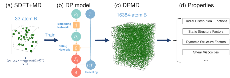
Figure 1: (Color online) Workflow of simulating WDM with the SDFT and DPMD methods. (a) We employ stochastic orbitals in SDFT to perform MD simulations on smaller systems (32 atoms in a bulk B) and collect initial training data, which include atomic positions, energies, forces, and virial tensors. (b) We utilize the gathered training data to construct a DP model with the temperature-dependent DPMD model. The deep neural network contains both embedding and fitting networks. (c) The new model enables us to perform simulations on large systems (16384 atoms) and at extremely high temperatures (350 eV). (d) Several physical quantities such as radial distribution functions, static structure factors, dynamic structure factors, and shear viscosities can be calculated, and the data are converged with large systems and long trajectories.

Recently, machine-learning-assisted atomistic simulation methods have achieved remarkable success and attracted considerable attention Behler (2011); Morawietz and Behler (2013); Bartók and Csányi (2015); Ko et al. (2019); Pun et al. (2019); Smith et al. (2019); Zeng et al. (2022); Gartner et al. (2020); Schörner et al. (2022a, b); Fiedler et al. (2022b); Kumar et al. (2023). In particular, deep neural networks are often adopted to learn the potential energy surfaces, which are formed by the relations between atomic configurations and their corresponding energies, forces, and stresses. Essentially, these neural-network-based models demonstrate high efficiency while maintaining ab initio accuracy, as they effectively bypass the need to solve quantum mechanics-based equations. Among them, the deep potential molecular dynamics (DPMD) method Zhang et al. (2018a); Wang et al. (2018); Zhang et al. (2020); Wen et al. (2022) achieves high performances Lu et al. (2021); Jia et al. (2020) and stands out as a promising method to study WDM. For example, the DPMD method has been applied to study the structural and dynamic properties of warm dense aluminum Liu, Lu, and Chen (2020); Zeng et al. (2021), the ion-ion dynamic structure factor of warm dense aluminum Zeng et al. (2021), the thermal transport by electrons and ions of warm dense aluminum Liu, Li, and Chen (2021), and the principal Hugoniot curves of warm dense beryllium Zhang et al. (2020), etc.

To summarize, two main challenges exist for large-scale first-principles simulations of WDM. First, the existence of the partial occupation of a large number of high-energy KS eigenstates results in computationally expensive simulations of WDM at high temperatures. Second, obtaining converged results for certain physical properties of WDM with a small number of atoms is difficult unless a large cell with a long MD trajectory is obtained. In this work, we first validate the accuracy of SDFT by analyzing the statistical errors from the stochastic orbitals and compare with results from the traditional KSDFT method. Here, we select warm dense boron (B) and carbon (C) as benchmark systems. Second, we couple the Born-Oppenheimer molecular dynamics (BOMD) method with SDFT to simulate warm dense B. Specifically, we generate two DP models to describe B at a density of 2.46 $\mathrm{g/cm^{3}}$ with two different temperatures (86 and 350 eV); the training data are obtained from SDFT-based BOMD simulations. Third, by performing DPMD simulations, we significantly extend the time and spatial scales of warm dense B and obtain converged data for certain physical properties. The above workflow is shown in Fig. 1. Our work demonstrates that combining SDFT with the deep potential (DP) method offers a promising route to simulate WDM over a wide range of temperatures.

The rest of the paper is organized as follows. Section II describes the computational methods utilized in this work. In Section III, we discuss the results obtained from SDFT and the DP model. Finally, we summarize our results in Section IV.

II Computational Methods

II.1 Stochastic and Mixed Stochastic-Deterministic Density Functional Theory

In the KSDFT framework Hohenberg and Kohn (1964); Kohn and Sham (1965), the single-particle DFT Hamiltonian is defined as

$$\hat{H}_{\mathrm{DFT}}=-\nabla^{2}/2+\hat{V}_{\mathrm{Hartree}}+\hat{V}_{\mathrm{xc}}+\hat{V}_{\mathrm{ext}},$$ (1)

where the first term depicts the kinetic operator, $\hat{V}_{\mathrm{Hartree}}$ denotes the Hartree potential, $\hat{V}_{\mathrm{xc}}$ is the exchange-correlation (XC) potential, and $\hat{V}_{\mathrm{ext}}$ is the potential of interactions between the electrons and the nuclei as well as other external fields. Within the finite-temperature Mermin-Kohn-Sham theory Mermin (1965), the electron density is given by

$$n(\mathbf{r}) =2\mathrm{Tr}\left[f\left(\hat{H}_{\mathrm{DFT}},\mu,T\right)\delta(\hat{\mathbf{r}}-\mathbf{r})\right]$$ (2)

$$=2\sum_{k=1}^{N_{k}}\omega_{k}\sum_{i=1}^{N_{\mathrm{KS}}}f\left(\varepsilon_{ik},\mu,T\right)\left|\phi_{ik}(\mathbf{r})\right|^{2},$$

where $\hat{\mathbf{r}}$ is the position operator of the electron, the prefactor 2 accounts for the electron spin. The parameter $\omega_{k}$ is the weight of the $k$ point with $N_{k}$ being the number of $k$ points, while $N_{\mathrm{KS}}$ is the number of occupied orbitals with $i$ being the index. The Fermi-Dirac distribution function takes the form of $f\left(\varepsilon_{ik},\mu,T\right)=1/[e^{(\varepsilon_{ik}-\mu)/T}+1]$, where $\mu$ is the chemical potential. Here, $\phi_{ik}(\mathbf{r})$ and $\varepsilon_{ik}$ respectively depict the eigenfunction and eigenvalue of the self-consistent KS Hamiltonian

$$\hat{H}_{\mathrm{DFT}}\phi_{ik}(\mathbf{r})=\varepsilon_{ik}\phi_{ik}(\mathbf{r}).$$ (3)

In practice, solving $\phi_{ik}(\mathbf{r})$ and $\varepsilon_{ik}$ is costly at high temperatures since the needed number of KS wave functions is proportional to $T^{\frac{3}{2}}$ Cytter et al. (2018).

Given any orthogonal and complete basis set $\{\psi_{j}\}$, a stochastic orbital $\chi_{nk}$ in SDFT Baer, Neuhauser, and Rabani (2013); Cytter et al. (2018) can be defined as

$$\left\langle\psi_{j}\mid\chi_{nk}\right\rangle=\frac{1}{\sqrt{N_{\mathrm{sto}}}}\exp\left(i2\pi\theta_{j}^{nk}\right),$$ (4)

which satisfies

$$\lim_{N_{\mathrm{sto}}\rightarrow+\infty}\sum_{n=1}^{N_{\mathrm{sto}}}\left|\chi_{nk}\right\rangle\left\langle\chi_{nk}\right|=\hat{I},$$ (5)

where $\theta_{j}^{nk}$ is randomly generated by a uniform distribution between 0 and 1, and $N_{\mathrm{sto}}$ is the number of stochastic orbitals.

In MDFT White and Collins (2020), both deterministic orbitals $\phi_{ik}$ and stochastic orbitals $\tilde{\chi}_{nk}$ are used,

$$\left|\tilde{\chi}_{nk}\right\rangle=\left|\chi_{nk}\right\rangle-\sum_{i=1}^{N_{\mathrm{KS}}}\left\langle\phi_{ik}\mid\chi_{nk}\right\rangle\left|\phi_{ik}\right\rangle.$$ (6)

Here, the stochastic orbitals are defined to be orthogonal to the deterministic orbitals. The number of deterministic orbitals is set to $N_{\mathrm{KS}}$, which is typically chosen to be a subset of occupied states. In addition, both sets of orbitals satisfy the relation

$$\lim_{N_{\mathrm{sto}}\rightarrow+\infty}\sum_{n=1}^{N_{\mathrm{sto}}}\left|\tilde{\chi}_{nk}\right\rangle\left\langle\tilde{\chi}_{nk}\right|+\sum_{i=1}^{N_{\mathrm{KS}}}\left|\phi_{ik}\right\rangle\left\langle\phi_{ik}\right|=\hat{I},$$ (7)

Then, the electron density is given by

$$n(\mathbf{r})=2\sum_{k=1}^{N_{k}}\omega_{k}\Bigg{[}\sum_{n=1}^{N_{\mathrm{sto}}}\left|\left\langle\mathbf{r}\left|\sqrt{f\left(\hat{H}_{\mathrm{DFT}},\mu,T\right)}\right|\chi_{nk}\right\rangle\right|^{2}$$ (8)

$$+\sum_{i=1}^{N_{\mathrm{KS}}}f\left(\varepsilon_{ik},\mu,T\right)\left|\phi_{ik}(\mathbf{r})\right|^{2}\Bigg{]},$$

where $\sqrt{f\left(\hat{H}_{\mathrm{DFT}},\mu,T\right)}$ is calculated by the Chebychev expansion Baer and Head-Gordon (1997). If $N_{\mathrm{sto}}=0$ or $N_{\mathrm{KS}}=0$, the MDFT method changes to the standard KSDFT or SDFT methods, respectively.

Notably, using stochastic orbitals in practical calculations results in statistical errors since these orbitals only form a complete basis when the number of stochastic orbitals approaches infinity. As reported in previous studies Fabian et al. (2019b); Baer, Neuhauser, and Rabani (2022); Liu and Chen (2022), the error caused by the stochastic orbitals is proportional to $1/\sqrt{N_{\mathrm{sto}}}$. However, when periodic boundary conditions (PBCs) with the $k$-point sampling are considered and each $k$-point has $N_{\mathrm{sto}}$ stochastic orbitals, the resulting $\sigma_{s}$ is proportional to $1/\sqrt{N_{k}N_{\mathrm{sto}}}$, suggesting that more $k$-points can reduce the stochastic errors. In order to evaluate the accuracy of SDFT, we perform both SDFT and KSDFT calculations for B and C bulk systems in extreme conditions.

In the first-principles MD simulations of WDM, the KSDFT couples with the dynamics of ions, usually through the BOMD method. Since the motions of ions are treated classically in the BOMD method, we need to evaluate the force of an atom $i$ in the form of

$$\mathbf{F}_{i}=-\frac{\partial E}{\partial\mathbf{R}_{i}}.$$ (9)

Here $E$ is the sum of electrons’ energy and ion-ion repulsion energy, and $\mathbf{R}_{i}$ is the position of atom $i$. By utilizing the plane-wave basis set and norm-conserving pseudopotentials within the traditional KSDFT and SDFT methods, the force of an atom can be decomposed into three parts

$$\mathbf{F}_{i}=\mathbf{F}_{i}^{L}+\mathbf{F}_{i}^{NL}+\mathbf{F}_{i}^{II},$$ (10)

where $\mathbf{F}_{i}^{L}$ is the local pseudopotential force term, $\mathbf{F}_{i}^{NL}$ depicts the nonlocal pseudopotential force term, and $\mathbf{F}_{i}^{II}$ is the Ewald force term origins from the ion-ion interactions. Furthermore, stress is defined as

$$\sigma_{\alpha\beta} =-\frac{1}{V}\frac{\partial E}{\partial\epsilon_{\alpha\beta}}$$ (11)

$$=\sigma_{\alpha\beta}^{T}+\sigma_{\alpha\beta}^{L}+\sigma_{\alpha\beta}^{NL}+\sigma_{\alpha\beta}^{\text{Hartree}}+\sigma_{\alpha\beta}^{\mathrm{xc}}+\sigma_{\alpha\beta}^{II},$$

where $\epsilon_{\alpha\beta}$ is the strain with the spatial coordinates $\alpha$ and $\beta$. The kinetic energy term of electrons is $\sigma_{\alpha\beta}^{T}$. $\sigma_{\alpha\beta}^{L}$ and $\sigma_{\alpha\beta}^{NL}$ are the local and nonlocal pseudopotential terms, respectively. $\sigma_{\alpha\beta}^{\text{Hartree }}$ is the Hartree and $\sigma_{\alpha\beta}^{\mathrm{xc}}$ is the exchange-correlation term. The Ewald term is $\sigma_{\alpha\beta}^{II}$. One can refer to Ref. Liu and Chen, 2022 by Liu et al. for more details on implementing the total energy, the total free energy, forces, and stresses within the framework of SDFT in ABACUS. Note that the SDFT method employed in this work still uses plane wave basis, so it is still computationally demanding for a system consisting of a few hundred atoms.

II.2 Deep Potential Molecular Dynamics

In the DPMD method Zhang et al. (2018b); Wang et al. (2018), the total energy $E$ of a system is expressed as a sum of atomic contributions, i.e., $E=\sum_{i}E_{i}$, where the energy $E_{i}$ from atom $i$ depends on an environment matrix $\mathcal{R}_{i}$, which includes the information of neighboring atoms of atom $i$ within a cutoff radius. The DP model maps $\mathcal{R}_{i}$ via an embedding neural network to a symmetry-preserving descriptor, and then the descriptor is mapped to a fitting neural network to yield $E_{i}$. A loss function is utilized to optimize the parameters in the embedding and fitting networks to generate DP models. The loss function is defined as

$$L(p_{\epsilon},p_{f},p_{\xi})=p_{\epsilon}\Delta\epsilon^{2}+\frac{p_{f}}{3N}\sum_{i}|\Delta\mathbf{F}_{i}|^{2}+\frac{p_{\xi}}{9}||\Delta\xi||^{2},$$ (12)

where $N$ is the number of atoms, $\epsilon=E/N$ is the energy per atom, $\mathbf{F}_{i}$ is the force acting on atom $i$, $\xi$ is the virial tensor per atom, and $\Delta$ denotes the difference between the training data and the results predicted by the DP model. In addition, $p_{\epsilon}$, $p_{f}$, and $p_{\xi}$ are tunable prefactors. The stochastic gradient descent scheme Adam Kingma and Ba (2017) is adopted to train the DP model.

We separately train the data from SDFT-based BOMD trajectories of B at 86 and 350 eV, where the Perdew-Burke-Ernzerhof (PBE) Perdew, Burke, and Ernzerhof (1996) functional is used. As a result, we obtain two DP models of warm dense B at the two temperatures. To better characterize the warm dense B at 350 eV, we adopt the temperature-dependent deep potential (TDDP) method Zhang et al. (2020) to train the DP model. Note that the TDDP method, as shown in Fig. 1(b), introduces the electron temperature of the system into the fitting net, which is more suitable for high-temperature systems.

Both embedding and fitting neural networks contain three layers with the specific number of neurons being (25, 50, 100) and (120, 120, 120), respectively. The cutoff radius for each atom is chosen to be 6.0 Å. The inverse distance $1/r$ decays smoothly from 0.5 to 6.0 Å in order to remove the discontinuity introduced by the cutoff. Both DP models undergo training for 500,000 steps. Throughout the training process, the values of $p_{\epsilon}$, $p_{f}$, and $p_{\xi}$ are gradually adjusted from 0.02 to 1, 1000 to 1, and 0.02 to 1, respectively. We also employ the DP compress technique to both DP models to accelerate the DPMD simulations, as described in the literature Lu et al. (2022).

III Results and Discussion

III.1 Statistical Errors of SDFT

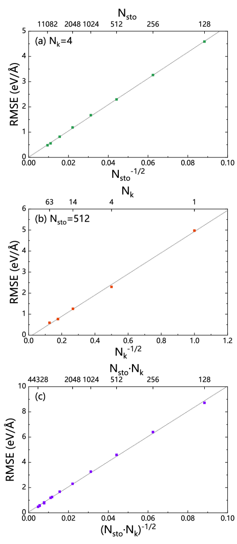
Figure 2: (Color online) Root-mean-square error (RMSE) of atomic forces arises from the SDFT calculations for B. The temperature is set to 350 eV and the density is set to 2.46 $\mathrm{g/cm^{3}}$. The RMSE is evaluated with respect to (a) the number of stochastic orbitals $N_{\mathrm{sto}}$, (b) the number of $k$ points in the Brillouin zone $N_{k}$, and (c) the product of $N_{\mathrm{sto}}$ and $N_{k}$. For each data point, the RMSE is obtained via 9 independent SDFT calculations with different sets of stochastic orbitals.

To analyze the statistical errors that arise from the SDFT method itself, we choose a 32-atom B system with a density of 2.46 $\mathrm{g/cm^{3}}$ at the temperature of 350 eV. In addition, we employ the PBE Perdew, Burke, and Ernzerhof (1996) exchange-correlation functional. We note that at the temperature of 86 eV and higher temperatures, the pseudopotential of B is generated by the ONCVPSP Hamann (2013) method with all of its 5 electrons. The cutoff radius for the pseudopotential is set to 0.7 Bohr to avoid overlaps of electron orbitals at high temperatures. In addition, we select an energy cutoff of 180, 240, and 300 Ry for temperatures of 86, 350, and 1000 eV, respectively.

Figure 2 shows the RMSE of SDFT verse the number of stochastic orbitals ($N_{\mathrm{sto}}$) and the number of $k$-point ($N_{k}$). For each data point in this figure, we label the average atomic force for each atom along a certain direction ($\gamma\in{x,y,z}$) as $\mathrm{F_{ave}}$, which is computed by averaging 9 independent SDFT calculations with different sets of stochastic orbitals. In each SDFT calculation, we label the force acting on each atom along the $\gamma$ direction as $\mathrm{F_{sto}}$. In this regard, the root-mean-square error (RMSE) can be evaluated via

$$\mathrm{RMSE}=\sqrt{\frac{1}{3N_{c}\cdot N}\sum_{c=1}^{N_{c}}\sum_{i=1}^{N}\sum_{\gamma}(\mathrm{F}_{\mathrm{sto}}-\mathrm{F}_{\mathrm{ave}})^{2}},$$ (13)

where $N_{c}=9$ is the number of independent SDFT runs, and $N=32$ is the number of atoms with $i$ being the index of atoms.

The number of stochastic orbitals is chosen from 128 to 11082 in Fig. 2(a), and the shifted $k$-point sampling is set to 2$\times$2$\times$2. Note that after symmetry analysis, the number of $k$ points reduces to 4 after symmetry analysis. We fix the number of stochastic orbitals to be 512 in Fig. 2(b) and choose the shifted $k$-point samplings of $1\times 1\times 1$ (1), $2\times 2\times 2$ (4), $3\times 3\times 3$ 32), and $5\times 5\times 5$ (65); here the number in the parentheses denotes the number of $k$-points after symmetry analysis. As expected, Figs. 2(a), (b), and (c) respectively show that the RMSE of forces acting on atoms exhibits linear behavior with respect to $N_{\mathrm{{sto}}}^{-1/2}$, $N_{k}^{-1/2}$, and $(N_{\mathrm{{sto}}}\times N_{k})^{-1/2}$. The numerical results are consistent with the discussion of statistical error in Section II.1. Importantly, the results indicate that as more stochastic orbitals and a larger number of $k$-point sampling are employed, the stochastic errors can be systematically mitigated.

III.2 Compare SDFT and KSDFT Results

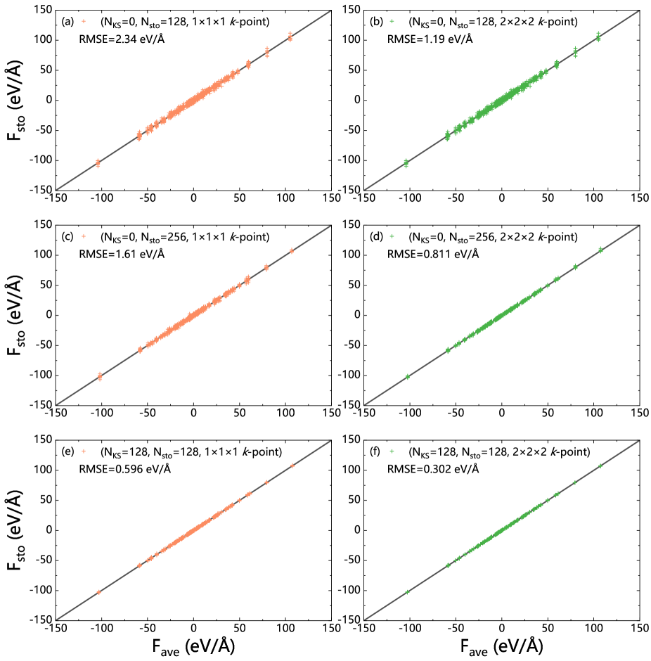
Figure 3: (Color online) Forces acting on each B atom as obtained from 9 independent SDFT calculations with different stochastic orbitals. The B system has a density of 2.46 $\mathrm{g/cm^{3}}$, and the temperature is 17.23 eV. For each calculation, the force acting on each atom along the $\gamma$ direction is denoted as $\mathrm{F_{sto}}$, and their average is $\mathrm{F_{ave}}$. $N_{\mathrm{{KS}}}$ refers to the number of KS orbitals, and $N_{\mathrm{{sto}}}$ is the number of stochastic orbitals. Two sets of Monkhorst-Pack $k$-points are utilized, i.e., a $1\times 1\times 1\ k$-point mesh (the $\Gamma\ k$-point) and a shifted $2\times 2\times 2\ k$-point mesh. The root-mean-square error (RMSE) of forces between $\mathrm{F_{sto}}$ and $\mathrm{F_{ave}}$ is computed via Eq. 13. The RMSE is obtained via the mentioned 9 independent SDFT calculations.

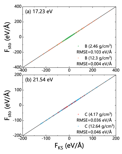
Figure 4: (Color online) (a) Comparison of forces acting on each B atom in a 32-atom cell with densities being 2.46 and 12.3 $\mathrm{g/cm^{3}}$ at a temperature of 17.23 eV. (b) Comparison of forces acting on each C atom with densities being 4.17 and 12.46 $\mathrm{g/cm^{3}}$ at a temperature of 21.54 eV. In the SDFT (KSDFT) calculation, we label the force acting on each atom along the $\gamma$ direction ($\gamma\in{x,y,z}$) as $\mathrm{F_{sto}}$ ($\mathrm{F_{KS}}$). The root-mean-square error (RMSE) of forces between $\mathrm{F_{sto}}$ and $\mathrm{F_{KS}}$ is listed.

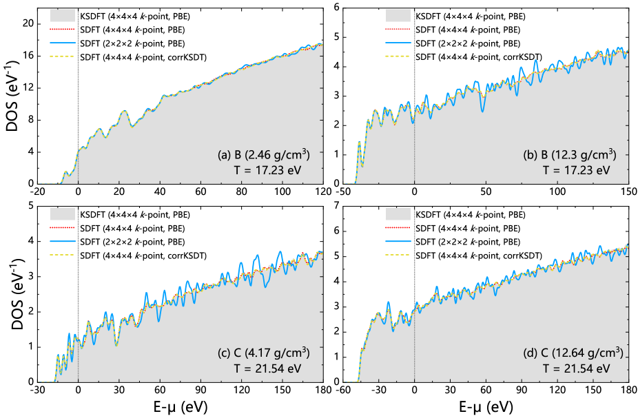
Figure 5: (Color online) Density of states (DOS) for the B and C systems as calculated by the SDFT and KSDFT methods. The densities are selected as (a) 2.46 $\mathrm{g/cm^{3}}$ and (b) 12.3 $\mathrm{g/cm^{3}}$ for B, and (c) 4.17 $\mathrm{g/cm^{3}}$ and (d) 12.64 $\mathrm{g/cm^{3}}$ for C systems. The Fermi energy is set to 0. We use two sets of $k$-point sampling in KSDFT and SDFT calculations. In addition, we adopt two exchange-correlation functionals, including PBE Perdew, Burke, and Ernzerhof (1996) and corrKSDT Karasiev, Dufty, and Trickey (2018).

Table 1: Comparison of the total energy per atom ($E$ in eV), the pressure ($P$ in GPa), and the degree of ionization ($\alpha$) for B and C systems as obtained from the SDFT and the traditional KSDFT methods. Four systems are chosen, i.e., two B systems at a temperature of 17.23 eV with densities being 2.46 and 12.3 $\mathrm{g/cm^{3}}$, and two C systems with densities being 4.17 and 12.46 $\mathrm{g/cm^{3}}$ at a temperature of 21.54 eV. $\Delta$ denotes the percentage difference between the results obtained by SDT and KSDFT.

		$E$ (eV)	$P$ (GPa)	$\alpha$
B	KSDFT	-153.683171	849.112	0.476617
2.46 $\mathrm{g/cm^{3}}$	SDFT	-153.707884	852.524	0.476659
17.23 eV	$\Delta$	0.0161%	0.4019%	0.0088%
B	KSDFT	-66.923177	8730.010	0.390341
12.3 $\mathrm{g/cm^{3}}$	SDFT	-66.924235	8730.829	0.390344
17.23 eV	$\Delta$	0.0016%	0.0094%	0.0008%
C	KSDFT	-263.586543	2018.380	0.505693
4.17 $\mathrm{g/cm^{3}}$	SDFT	-263.595810	2019.780	0.505707
21.54 eV	$\Delta$	0.0035%	0.0693%	0.0028%
C	KSDFT	-190.692843	9168.050	0.440747
12.46 $\mathrm{g/cm^{3}}$	SDFT	-190.698535	9171.552	0.440757
21.54 eV	$\Delta$	0.0030%	0.0382%	0.0023%

In order to select suitable numbers of $k$-points, KS orbitals, and stochastic orbitals for simulating warm dense matter under specific conditions, we use a 32-atom B system as an example, with a density of 2.46 $\mathrm{g/cm^{3}}$ and a temperature of 17.23 eV. Figure 3 compares the forces on each B atom with different values for the mentioned parameters. First, we find that increasing the $k$-point sampling size from the $\Gamma$ point to a shifted $2\times 2\times 2$ $k$-point sampling substantially reduces the RMSE, which is consistent across various values of $N_{\mathrm{KS}}$ and $N_{\mathrm{sto}}$. The result is in line with the linear relationship shown in Fig. 2. Second, we note that the RMSE with $N_{\mathrm{KS}}=0$ and $N_{\mathrm{sto}}=256$ in Fig. 3(c) is 1.61 eV/ Å , while the RMSE with $N_{\mathrm{KS}}=128$ and $N_{\mathrm{sto}}=128$ shown in Fig. 3(e) is 0.596 eV/ Å . The former is considerably larger than the latter, suggesting that increasing the number of KS orbitals is more effective than using stochastic orbitals at a relatively low temperature (17.23 eV). Consequently, by choosing an adequate number of KS orbitals ($N_{\mathrm{KS}}=128$) and stochastic orbitals ($N_{\mathrm{sto}}=128$) along with the shifted $2\times 2\times 2$ $k$-point sampling, we can achieve an RMSE as small as 0.302 eV/ Å . Furthermore, we examine the effects of these parameters on B systems at 86 and 350 eV, with the results shown in Figs. S1 and S2 of Supporting Information (SI), respectively. In conclusion, we find it reasonable to select the same parameters as in the B system at 17.23 eV.

Next, Table 1 presents a comparison of some key physical properties obtained from the SDFT and KSDFT methods. Specifically, we evaluate the total energy per atom ($E$), the pressure ($P$), and the degree of ionization ($\alpha$). $\Delta$ is the percentage difference between the results obtained from SDFT and the traditional KSDFT. We consider four systems, including two B systems at a temperature of 17.23 eV and densities of 2.46 and 12.3 $\mathrm{g/cm^{3}}$, as well as two C systems at a temperature of 21.54 eV and densities of 4.17 and 12.46 $\mathrm{g/cm^{3}}$. In both SDFT and KSDFT calculations, we choose the PBE Perdew, Burke, and Ernzerhof (1996) functional. Furthermore, a shifted $2\times 2\times 2$ $k$-point sampling grid is adopted.

We study B systems with a cell containing 32 atoms. Additionally, we employ a norm-conserving pseudopotential for B with 3 valence electrons Schlipf and Gygi (2015), and the energy cutoff is 150 Ry. We respectively set the number of deterministic orbitals in KSDFT to be $N_{\mathrm{KS}}=992$ and 400 for the B systems with density being 2.46 and 12.3 $\mathrm{g/cm^{3}}$. This setting ensures the occupation of electrons to be smaller than $10^{-4}$ at the highest-energy orbital. On the other hand, we choose the number of deterministic orbitals to be $N_{\mathrm{KS}}=240$ and the number of stochastic orbitals to be $N_{\mathrm{sto}}=120$ in SDFT for the B systems regardless of their densities. Regarding the C systems, a norm-conserving pseudopotential with 4 valence electrons is employed Schlipf and Gygi (2015), and the energy cutoff is set to 160 Ry. We utilize 8 (32) atoms in a cell and $N_{\mathrm{KS}}=350\ (520)$ for a density of 4.17 (12.46) $\mathrm{g/cm^{3}}$ in KSDFT calculations. In SDFT calculations, we adopt $N_{\mathrm{KS}}=120\ (240)$ and $N_{\mathrm{sto}}=120\ (120)$ for 4.17 (12.46) $\mathrm{g/cm^{3}}$.

As shown in Table 1, we have the following findings. First, it can be seen that the percentage difference in total energy ($\Delta$ of $E$) between SDFT and KSDFT is relatively small, being less than 0.02% for the B systems and 0.004% for the C systems. This indicates that SDFT provides a high-accuracy estimation of total energy when compared to the conventional KSDFT method. Second, the percentage difference in pressure ($\Delta$ of $P$) between the two methods is smaller than 0.41% for B and 0.07% for C. This further supports the high accuracy of the SDFT method. Third, the ionization process of electrons plays a crucial role in determining the WDM equation of state Gao et al. (2016); Zhang et al. (2018c); Blanchet et al. (2022b). This process can be represented by the degree of ionization, denoted as $\alpha$. In practice, the Fermi energy of the system at 0 K is defined as $\mu$. Consequently, the degree of ionization $\alpha$ at a finite temperature $T$ can be defined as follows

$$\alpha=1-\frac{N_{T,occ}}{N_{0,occ}},$$ (14)

where $N_{T,occ}$ is the total number of occupied electrons below $\mu$ when the electrons follow the Fermi-Dirac distribution at tempearture $T$. In addition, $N_{0,occ}$ is a special case of $N_{T,occ}$ when $T=0$. The percentage difference in the degree of ionization ($\Delta$ of $\alpha$) is found to be smaller than 0.009% for both B and C systems. In summary, all three properties, namely $E$, $P$, and $\alpha$ calculated by SDFT show excellent accuracy when compared to those from the traditional KSDFT. This demonstrates that SDFT is a reliable method for simulating high-temperature materials with first-principles accuracy.

Fig. 4 further compares the forces acting on each atom of B (2.46 and 12.3 $\mathrm{g/cm^{3}}$) and C (4.17 and 12.46 $\mathrm{g/cm^{3}}$) obtained from both SDFT and KSDFT calculations. We find that the forces predicted by SDFT are in excellent agreement with those from KSDFT. For instance, the RMSE of forces is smaller than 0.05 eV/Å for both C systems. The largest RMSE occurs in the B system at 2.46 $\mathrm{g/cm^{3}}$, with a value of 0.103 eV/Å, which is relatively small compared to the magnitude of atomic forces (a few hundreds of eV/Å). Notably, we find the smallest RMSE is 0.004 eV/Å in the B system at 12.3 $\mathrm{g/cm^{3}}$. This is due to the fact that more electronic states of B are occupied by electrons at this condition, as demonstrated by the smaller degree of ionization of B (0.39) shown in Table. 1.

Fig. 5 illustrates the DOS of B (2.46 and 12.3 $\mathrm{g/cm^{3}}$) and C (4.17 and 12.46 $\mathrm{g/cm^{3}}$). Besides the PBE Perdew, Burke, and Ernzerhof (1996) exchange-correlation functional, we also test the finite-temperature local density approximation functional, i.e., the corrKSDT functional as proposed by Karasiev et al. Karasiev, Dufty, and Trickey (2018). A Monkhorst-Pack $4\times 4\times 4$ shifted $k$-point mesh is adopted in KSDFT calculations to yield the DOS of B and C. However, unlike the traditional KSDFT method, DOS in SDFT cannot be directly obtained from the eigenvalues of $\hat{H}$. Instead, we evaluate the DOS from the SDFT method via the following formula

$$g(E)=2\operatorname{Tr}\left[\frac{1}{\sqrt{2\pi}\sigma}\exp\left(-\frac{(E-\hat{H})^{2}}{2\sigma^{2}}\right)\right].$$ (15)

Here, $\sigma$ depicts the width of smearing. The DOS of SDFT with a shifted $2\times 2\times 2$ $k$-point mesh converges for B with a density of 2.46 $\mathrm{g/cm^{3}}$ when compared with KSDFT, although there are some deviations observed in the other three cases. Notably, the DOS predicted by SDFT using a $4\times 4\times 4$ shifted $k$-point mesh shows excellent agreement with the KSDFT results for both B and C systems. By employing a shifted $4\times 4\times 4$ $k$-point mesh, it is also observed that the DOS of corrKSDT Karasiev, Dufty, and Trickey (2018) exhibits no significant differences when compared with the PBE Perdew, Burke, and Ernzerhof (1996) results, suggesting that the temperature effects in the XC functional have minimal impacts on our calculations. Overall, these findings indicate that the SDFT implemented in ABACUS is adequately accurate for simulating warm dense B and C systems.

III.3 High-Temperature Calculations by SDFT

Table 2: Root-Mean-Square Error (RMSE) of forces acting on B atoms as obtained from 9 independent SDFT calculations with two sets of stochastic orbitals (128 and 256). The B system has a density of 2.46 $\mathrm{g/cm^{3}}$, and the temperatures are set to 17.23, 86, 350, and 1000 eV. $N_{\mathrm{{KS}}}$ refers to the number of KS orbitals, and $N_{\mathrm{{sto}}}$ is the number of stochastic orbitals. Two sets of Monkhorst-Pack $k$-points are utilized, i.e., a $1\times 1\times 1\ k$-point mesh (include the $\Gamma\ k$-point) and a shifted $2\times 2\times 2\ k$-point mesh. The RMSE of forces is computed via Eq. 13.

T (eV)	$N_{\mathrm{KS}}$	$N_{\mathrm{sto}}$	$k$ points	RMSE (eV/Å)
17.23	128	128	$1\times 1\times 1$	0.596
	128	128	$2\times 2\times 2$	0.302
86	128	128	$1\times 1\times 1$	3.26
	128	128	$2\times 2\times 2$	1.54
350	0	256	$1\times 1\times 1$	6.40
	0	256	$2\times 2\times 2$	3.26
1000	0	256	$1\times 1\times 1$	2.68
	0	256	$2\times 2\times 2$	1.30

Table 2 collects the three force components of each atom in the 32-atom B cell from 9 independent runs of SDFT with different stochastic orbitals. Four different temperatures are chosen, i.e., 17.23, 86, 350, and 1000 eV. Furthermore, we select $1\times 1\times 1$ and $2\times 2\times 2$ shifted $k$-point samplings for each temperature and evaluate the corresponding RMSE. At each condition, a set of average forces $\mathrm{F}_{\mathrm{ave}}$ are calculated according to Eq. 13. One can refer to Fig. S3 of SI for more details. For temperatures of 17.23 and 86 eV, we set $N_{\mathrm{KS}}=128$ and $N_{\mathrm{sto}}=128$; at higher temperatures of 350 and 1000 eV, we find it more effective to use stochastic orbitals than the KS orbitals. As a result, we do not choose the Kohn-Sham orbitals ($N_{\mathrm{KS}}=0$) but set all orbitals to be stochastic orbitals ($N_{\mathrm{sto}}=256$). According to our tests, the RMSE of the atomic force smaller than 3.3 eV/Å is enough for FPMD simulations of WDM B. Therefore, we employ the $\Gamma\ k$-point with 128 KS orbitals and 128 stochastic orbitals for 86 eV and the $2\times 2\times 2$ shifted $k$-point with 256 stochastic orbitals for 350 eV to perform FPMD.

III.4 Radial Distribution Functions

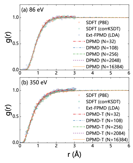
Figure 6: (Color online) Radial distribution functions $g(r)$ of B systems with a density of 2.46 $\mathrm{g/cm^{3}}$ at temperatures of (a) 86 eV and (b) 350 eV. The $g(r)$ obtained by Ext-FPMD with the LDA functional comes from Blanchet et al. Blanchet et al. (2022b) The SDFT calculations are performed with the PBE Perdew, Burke, and Ernzerhof (1996) and corrKSDT Karasiev, Dufty, and Trickey (2018) exchange-correlation functionals. The number of B atoms is set to 32 in the first-principles molecular dynamics simulations. DPMD depicts the model trained by the traditional DP method Wang et al. (2018), while DPMD-T means the model trained by the TDDP method Zhang et al. (2020). $N$ is the number of B atoms in a cell, which ranges from 32 to 16384 in the deep-potential-based simulations.

Previous works have employed the traditional KSDFT coupling with BOMD to study WDM at relatively low temperatures. The examples include the shock Hugoniot curves Militzer et al. (2021), the radial distribution function Driver and Militzer (2012); Liu, Lu, and Chen (2020), the ion-ion static structure factor Liu, Lu, and Chen (2020), and the ion-ion dynamic structure factor Liu, Lu, and Chen (2020); Zeng et al. (2021), etc. However, most of these calculations are limited due to the high computational costs of dealing with electrons at extremely high temperatures. In order to substantially accelerate the calculations, we choose the DPMD method to perform BOMD calculations for warm sense B systems, and the training data are obtained from efficient SDFT calculations for warm dense B at temperatures of 86 and 350 eV. Note that we use the traditional DP method Wang et al. (2018) to train the data at a temperature of 86 eV. However, we utilize the TDDP method Zhang et al. (2020) and include the electron temperature as an input parameter of the neural network to train the high-temperature data (350 eV), which shows a better performance than the traditional DP method at such a high temperature.

In detail, we perform SDFT-based BOMD simulations for a 32-atom B system with a density of 2.46 $\mathrm{g/cm^{3}}$. At the temperature of 86 eV, we adopt a $\Gamma\ k$-point mesh with the number of Kohn-Sham orbitals being $N_{\mathrm{KS}}=128$ and the number of stochastic orbitals being $N_{\mathrm{sto}}=128$. For a higher temperature of 350 eV, a $2\times 2\times 2$ shifted $k$-point mesh is used with the number of stochastic orbitals being $N_{\mathrm{sto}}=256$. We note that convergence with respect to the plane-wave energy cutoff and $k$-point mesh is examined to ensure the computational error of the total energy is within 0.01%. The BOMD simulations are performed in the NVT ensemble with the ion temperature controlled by the velocity-rescaling thermostat. The electrons and ions in the system are set to the same temperature. The time step is chosen according to $\Delta{t}\sim 1/\left(\rho^{1/3}T_{e}^{1/2}\right)$, where $T_{e}$ is the temperature of electrons and $\rho$ is the density. As a result, the time step is chosen to be 0.035 and 0.007 fs for simulations at 86 and 350 eV, respectively. In each BOMD trajectory, 4000 MD steps are performed. We then collect the atomic positions, the total energies $E$, the atomic forces $\mathbf{F}_{i}$ of each atom $i$, as well as the virial tensors $\Xi$ as the training data to generate DP models for B. Although stochastic DFT exhibits favorable scalability with increasing atoms Baer, Neuhauser, and Rabani (2013), previous research Zhang et al. (2019); Zeng et al. (2020); Zhang et al. (2020); Chen et al. (2023) suggests that having 32 Boron atoms in the training dataset is enough to generate an accurate deep potential. The use of 32 Boron atoms to generate the training set is a choice that balances efficiency and accuracy.

In DPMD simulations, we adopt the NVT ensemble with the Nosé-Hoover thermostat Nosé (1984); Hoover (1985). We use the LAMMPS package Plimpton (1995). The number of B atoms ranges from 32 to 16384. A time step of 0.07 fs is set for the system at 86 eV and 0.01 fs for the system at 350 eV. We perform 400000 steps of DPMD simulations to yield the radial distribution functions, the static structure factors, and the dynamic structure factors. Furthermore, one million MD steps are performed to compute the shear viscosity.

After the BOMD trajectories are generated, the radial distribution function can be evaluated according to

$$g(r)=\frac{V}{4\pi r^{2}N(N-1)}\bigg{\langle}\sum_{i=1}^{N}\sum_{j=1,j\neq i}^{N}\delta(r-|\mathbf{r}_{i}-\mathbf{r}_{j}|)\bigg{\rangle},$$ (16)

where $V$ is the cell volume, $N$ is the number of atoms, $\mathbf{r}_{i}$ and $\mathbf{r}_{j}$ are atomic coordinates of atoms $i$ and $j$, and $\langle\cdots\rangle$ means the the ensemble average. We plot $g(r)$ of warm dense B with a density of 2.46 $\mathrm{g/cm^{3}}$ at 86 and 350 eV in Fig. 6. We use Ext-FPMD Blanchet et al. (2022b), SDFT with two different XC functionals (PBE and corrKSDT), and DPMD methods to perform BOMD simulations. We have the following findings. First, we find that the SDFT results are in excellent agreement with those obtained from Ext-FPMD. Second, there are no substantial differences between the PBE Perdew, Burke, and Ernzerhof (1996) and the finite-temperature XC functional corrKSDT Karasiev, Dufty, and Trickey (2018), which indicates that temperature effects in the exchange-correlation functional are not significant. Third, as expected, the $g(r)$ is not smooth due to a limited number of MD steps (4000). However, by employing the DPMD method, we not only achieve accurate $g(r)$ that agree well with the SDFT results but also obtain a smooth $g(r)$, as a larger number of atoms (108 to 16384) and a longer trajectory (400000 steps) are considered. Importantly, size effects can be largely mitigated, as evidenced by the convergence of the $g(r)$ at around 108 atoms.

III.5 Ion-Ion Static Structure Factors

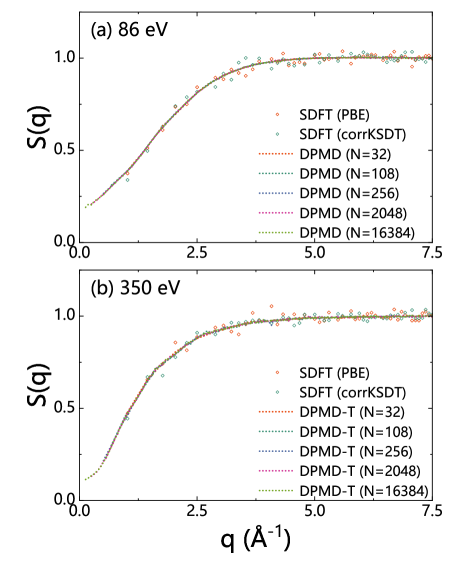
Figure 7: (Color online) Static structure factors $S(q)$ of B with a density of 2.46 $\mathrm{g/cm^{3}}$ at temperatures of (a) 86 eV and (b) 350 eV. The SDFT calculations are performed with the PBE Perdew, Burke, and Ernzerhof (1996) and corrKSDT Karasiev, Dufty, and Trickey (2018) exchange-correlation functionals. The number of B atoms is set to 32 in the first-principles molecular dynamics simulations. DPMD depicts the model trained by the traditional DP method Wang et al. (2018), while DPMD-T indicates the model trained by the TDDP method Zhang et al. (2020). $N$ is the number of B atoms in a cell ranging from 32 to 16384 in the deep-potential-based simulations.

The ion-ion static structure factor $S(q)$ measured from diffraction experiments Greenfield, Wellendorf, and Wiser (1971); Svensson et al. (1980) contains information regarding the spatial arrangement of particles in a material. The formula of $S(q)$ is

$$S(q)=\frac{1}{N}\left\langle\sum_{i=1}^{N}\sum_{j=1}^{N}e^{i\mathbf{q}\cdot\left(\mathbf{r}_{i}-\mathbf{r}_{j}\right)}\right\rangle,$$ (17)

where $N$ is the number of atoms, while $i$, $j$ denote atoms, and $q$ is a wave vector. Here, we perform BOMD simulations on a 32-atom cell by SDFT with the PBE Perdew, Burke, and Ernzerhof (1996) and corrKSDT Karasiev, Dufty, and Trickey (2018) exchange-correlation functionals. Moreover, we employ DPMD to calculate the $S(q)$ for cells containing 32, 108, 256, 2048, and 16384 B atoms with a density of 2.46 $\mathrm{g/cm^{3}}$. The results for systems at 86 and 350 eV are illustrated in Figs. 7(a) and (b), respectively. It is noteworthy that the data points of $S(q)$ generated by SDFT exhibit oscillations due to the limited number of MD steps (4000). However, the DPMD simulations offer more converged results as they allow for a larger cell size with considerably more atoms and a substantially longer trajectory in BOMD simulations. Furthermore, with the use of larger cells in DPMD, we can obtain reasonable low-$q$ information of $S(q)$, which signifies the long-ranged order of systems.

III.6 Ion-Ion Dynamic Structure Factors

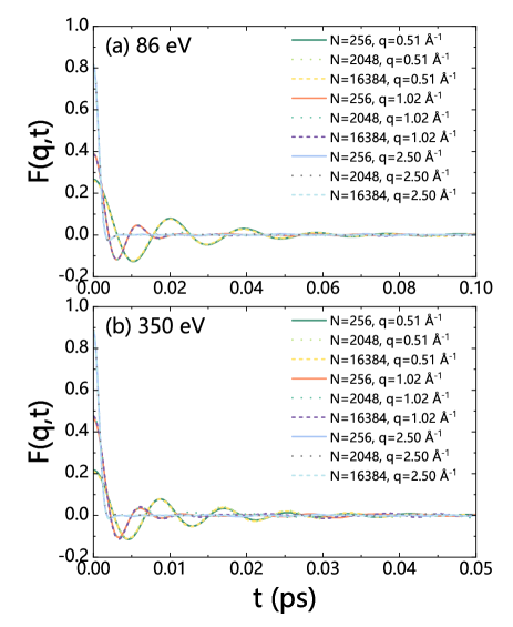
Figure 8: (Color online) Intermediate scattering functions $F(q,t)$ of B with a density of 2.46 $\mathrm{g/cm^{3}}$ as calculated from DPMD trajectories. Three system sizes (256, 2048, and 16384 atoms) are adopted in DPMD simulations at two temperatures of (a) 86 eV and (b) 350 eV. Three wave vectors are chosen, i.e., $q$=0.51, 1.02, and 2.50 Å^-1.

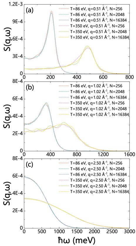
Figure 9: (Color online) Ion-ion dynamic structure factors $S(q,\omega)$ of B with a density of 2.46 $\mathrm{g/cm^{3}}$ as computed from DPMD trajectories. Three system sizes (256, 2048, and 16384 atoms) are adopted. The wave vectors are chosen to be (a) $q$=0.51 Å^-1, (b) 1.02 Å^-1, and (c) 2.50 Å^-1.

The collective dynamics of ionic density fluctuations can be characterized by the ion-ion dynamic structure factor $S(q,\omega)$, which is experimentally measurable Kählert (2019) and plays a crucial role in investigating ion dynamics, including collective modes Giordano and Monaco (2010), dissipation processes Mabey et al. (2017), and others. In practice, $S(q,\omega)$ can be computed from the intermediate scattering function $F(q,t)$ via Fourier transform with the formula being

$$S(q,\omega)=\frac{1}{2\pi}\int_{-\infty}^{+\infty}F(q,t)e^{i\omega t}\mathrm{~{}d}t.$$ (18)

Here $F(q,t)$ takes the form of

$$F(q,t)=\frac{1}{N}\langle\rho(\mathbf{q},t)\rho(-\mathbf{q},0)\rangle,$$ (19)

where $N$ is the number of ions, $\rho(\mathbf{q},t)$ is defined as

$$\rho(\mathbf{q},t)=\sum_{i=1}^{N}e^{i\mathbf{q}\cdot\mathbf{r}_{i}(t)},$$ (20)

where $\mathbf{r}_{i}(t)$ is the atomic coordinates for atom $i$ at time $t$.

Figs. 8(a) and (b) illustrate the intermediate scattering function $F(q,t)$ of warm dense B at 86 and 350 eV, respectively. Three wave vectors are chosen ($q$=0.51, 1.02, and 2.50) while three sizes of cells are tested (256, 2048, and 16384 atoms). We find the 256-atom cell is large enough to converge $F(q,t)$ for both temperatures, which is beyond the capabilities of SDFT-based BOMD simulations.

Next, we obtain the ion-ion dynamics structure factors $S(q,\omega)$ of warm dense B by performing the Fourier transform of $F(q,t)$. The results associated with wave vectors $q$ being 0.51, 1.02, and 2.50 Å^-1 are shown in Figs. 9(a), (b), and (c), respectively. In each figure, two temperatures (86 and 350 eV) and three system sizes (256, 2048, and 16384 atoms) are adopted. For the wave vector, $q$=0.51 Å^-1, Fig. 9(a) shows the well-pronounced ion-acoustic modes located at $\omega$ = 206.78 meV for 86 eV and 486.80 meV for 350 eV. When $q$ increases to 1.02 Å^-1 in Fig. 9(b), the peak of $S(q,\omega)$ becomes lower, and its location turns to 324.95 meV for 86 eV and 616.53 meV for 350 eV. Notably, the ion-acoustic mode $S(q,\omega)$ disappears when $q$ = 2.50 Å^-1, because the non-collective mode dominates at large $q$. The above results of $S(q,\omega)$ demonstrate that the DP method can predict the long-ranged structural and time correlation of WDM. For high temperatures up to hundreds of eV, there are experimental measurements of the ion-ion static structure factors and dynamic structure factors via X-ray Thomson scattering for materials, such as CH Kraus et al. (2016) and Be Döppner et al. (2023). To the best of our knowledge, no experimental data are available for B at the temperatures of 86 and 350 eV.

III.7 Shear Viscosities

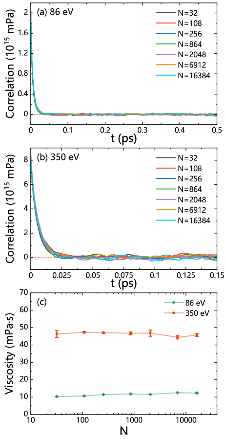
Figure 10: (Color online) Stress auto-correlation functions (Eq. 21) of warm dense B with a density of 2.46 $\mathrm{g/cm^{3}}$ at temperatures of (a) 86 eV and (b) 350 eV. (c) Shear viscosity of B. We use DPMD simulations with the cells containing 32, 108, 256, 864, 2048, 6912, and 16384 atoms. Error bars represent the standard deviations.

The shear viscosity is a crucial parameter in WDM studies, but obtaining a converged viscosity using traditional first-principles molecular dynamics is computationally expensive. However, this challenge can be significantly mitigated by employing the DPMD method with the training data from the SDFT method. One way to compute the shear viscosity $\eta$ of WDM is using the Green-Kubo relations Green (1954); Kubo (1957), which links the shear viscosity to the integral of the stress auto-correlation function with the form of

$$\eta=\frac{V}{3k_{B}T}\int_{0}^{+\infty}\left(\sum_{\alpha\beta}\left\langle P_{\alpha\beta}(0)P_{\alpha\beta}(t)\right\rangle\right)\mathrm{~{}d}t,$$ (21)

where $V$ is the volume of the system, $T$ is the temperature, $k_{B}$ is the Boltzmann constant, and $P_{\alpha\beta}(t)$ ($\alpha\beta\in\{xy,xz,yz\}$) is any of the three independent off-diagonal elements of the stress tensor at time $t$. The above formula can be used when DPMD trajectories are generated with the stress tensors.

The calculated stress auto-correlation functions of B at a density of 2.46 $\mathrm{g/cm^{3}}$ and temperatures of 86 and 350 eV are displayed in Figs. 10(a) and (b), respectively. In practice, the computed shear viscosity may be affected by the system size and the trajectory length of molecular dynamics simulations. Therefore, we choose seven different system sizes with the number of atoms per cell ranging from 32 to 16384. During DPMD simulations, each system is first relaxed for 50000 steps. Next, 1 million steps of MD simulations are performed to calculate the stress auto-correlation function. In detail, the trajectory length is 70 ps for 86 eV and 10 ps for 350 eV. We take values from 0.105 to 0.305 ps (0.05 to 0.1 ps) to compute the averaged shear viscosity for the system at 86 eV (350 eV), and the predicted values are shown in Fig. 10(c) with small error bars. As a result, the obtained shear viscosity of B varies from 10.3 to 12.3 $\mathrm{mPa\cdot s}$ at 86 eV and from 44.4 to 47.3 $\mathrm{mPa\cdot s}$ at 350 eV. The above results show no substantial finite-size effects for the shear viscosity of B, which is consistent with previous conclusions Chen et al. (2015); Vella et al. (2017); Malosso et al. (2022).

There are other formulas that can predict the shear viscosity of materials. For example, we notice that a recent work proposes an extended random-walk shielding-potential viscosity model (ext-RWSP-VM) Cheng et al. (2022, 2023) to elevate the shear viscosity of materials in WDM and HDP states. The viscosity is evaluated by the formula of

$$\eta=\frac{\sqrt{3mk_{B}T}}{\pi d^{4}}I,$$ (22)

where $d$ is the collision diameter introduced by hard-sphere concept, and $I$ is a quantity that is relevant to $T$. According to the ext-RWSP-VM method, we obtain the viscosities of B to be 12.8 and 47.8 $\mathrm{mPa\cdot s}$ for temperatures of 86 and 350 eV, respectively. More details can be found in SI. Interestingly, the data are close to our first-principles results. In addition, we find the shear viscosity of plasma can also be described by the approximate formula Maher I. Boulos (2023) of

$$\eta=\frac{2}{3\sqrt{\pi}}\frac{\sqrt{mk_{B}T}}{\sigma_{o}},$$ (23)

where $m$ is the atomic mass and $\sigma_{o}$ is the total collision cross section ($\sim 10^{-20}\mathrm{m^{2}}$). Thus, the estimated shear viscosities of B are around $\sim$ 18.7 and 37.8 $\mathrm{mPa\cdot s}$ for temperatures of 86 and 350 eV, respectively. It should be noted that $\sigma_{o}$ in the approximate formula is assumed to be a constant; however, it is related to the relative velocity between atoms Maher I. Boulos (2023). As the relative velocity increases, the interaction time decreases, leading to a reduced probability of collisions occurring. In other words, $\sigma_{o}$ decreases with increasing temperature. We find that the calculated shear viscosities from DPMD are also consistent with the approximated values obtained using Eq. 23.

IV Conclusions

Simulating WDM with first-principles accuracy had long been challenging due to the existence of the partial occupation of a large number of high-energy KS eigenstates and the resulting limitations in the time and space scales. Our work suggested that the advent of the SDFT method and machine-learning-based molecular dynamics can be of great help in overcoming the difficulties. The SDFT method described in this work had been implemented with the plane-wave basis set and the $k$-point sampling method, which was enabled in the ABACUS package (https://github.com/deepmodeling/abacus-develop). In this work, we validated the SDFT-based BOMD method by performing a series of tests for warm dense B and C.

By combining SDFT with the DP method, we substantially extended the time and space scales of simulating warm dense B and reduced the finite size effect. Besides, we studied the structural properties, dynamic properties, and transport coefficients, such as radial distribution functions, static structure factors, ion-ion dynamic structure factors, and shear viscosities. This work validated combining stochastic density functional theory with machine learning techniques to study high-temperature systems. We also offered new insights into the properties of warm dense matter. In future work, we intend to explore the generation of training data with a larger number of atoms. Future research may further refine these methods and expand their applicability to other materials and temperature ranges.

References

- Guillot (1999) T. Guillot, “Interiors of giant planets inside and outside the solar system,” Science 286, 72–77 (1999).
- Campbell et al. (2017) E. Campbell, V. Goncharov, T. Sangster, S. Regan, P. Radha, R. Betti, J. Myatt, D. Froula, M. Rosenberg, I. Igumenshchev, W. Seka, A. Solodov, A. Maximov, J. Marozas, T. Collins, D. Turnbull, F. Marshall, A. Shvydky, J. Knauer, R. McCrory, A. Sefkow, M. Hohenberger, P. Michel, T. Chapman, L. Masse, C. Goyon, S. Ross, J. Bates, M. Karasik, J. Oh, J. Weaver, A. Schmitt, K. Obenschain, S. Obenschain, S. Reyes, and B. Van Wonterghem, “Laser-direct-drive program: Promise, challenge, and path forward,” Matter Radiat. at Extremes 2, 37–54 (2017).
- Moses (2009) E. I. Moses, “Ignition on the national ignition facility: a path towards inertial fusion energy,” Nucl. Fusion 49, 104022 (2009).
- Graziani et al. (2014) F. Graziani, M. P. Desjarlais, R. Redmer, and S. B. Trickey, “Frontiers and challenges in warm dense matter,” (Springer Cham, 2014).
- Remington, Drake, and Ryutov (2006) B. A. Remington, R. P. Drake, and D. D. Ryutov, “Experimental astrophysics with high power lasers and pinches,” Rev. Mod. Phys. 78, 755–807 (2006).
- Hohenberg and Kohn (1964) P. Hohenberg and W. Kohn, “Inhomogeneous electron gas,” Phys. Rev. 136, B864–B871 (1964).
- Kohn and Sham (1965) W. Kohn and L. J. Sham, “Self-consistent equations including exchange and correlation effects,” Phys. Rev. 140, A1133–A1138 (1965).
- Militzer and Ceperley (2000) B. Militzer and D. M. Ceperley, “Path integral monte carlo calculation of the deuterium hugoniot,” Phys. Rev. Lett. 85, 1890–1893 (2000).
- Militzer et al. (2001) B. Militzer, D. M. Ceperley, J. D. Kress, J. D. Johnson, L. A. Collins, and S. Mazevet, “Calculation of a deuterium double shock hugoniot from ab initio simulations,” Phys. Rev. Lett. 87, 275502 (2001).
- Hu et al. (2010) S. X. Hu, B. Militzer, V. N. Goncharov, and S. Skupsky, “Strong coupling and degeneracy effects in inertial confinement fusion implosions,” Phys. Rev. Lett. 104, 235003 (2010).
- Driver and Militzer (2012) K. P. Driver and B. Militzer, “All-electron path integral monte carlo simulations of warm dense matter: Application to water and carbon plasmas,” Phys. Rev. Lett. 108, 115502 (2012).
- Wang, He, and Zhang (2011) C. Wang, X.-T. He, and P. Zhang, “Ab initio simulations of dense helium plasmas,” Phys. Rev. Lett. 106, 145002 (2011).
- White et al. (2013) T. G. White, S. Richardson, B. J. B. Crowley, L. K. Pattison, J. W. O. Harris, and G. Gregori, “Orbital-free density-functional theory simulations of the dynamic structure factor of warm dense aluminum,” Phys. Rev. Lett. 111, 175002 (2013).
- Kang et al. (2020) D. Kang, K. Luo, K. Runge, and S. B. Trickey, “Two-temperature warm dense hydrogen as a test of quantum protons driven by orbital-free density functional theory electronic forces,” Matter Radiat. at Extremes 5, 064403 (2020).
- Liu, Lu, and Chen (2020) Q. Liu, D. Lu, and M. Chen, “Structure and dynamics of warm dense aluminum: a molecular dynamics study with density functional theory and deep potential,” J. Phys. Condens. Matter 32, 144002 (2020).
- Zhang et al. (2016) S. Zhang, H. Wang, W. Kang, P. Zhang, and X. T. He, “Extended application of kohn-sham first-principles molecular dynamics method with plane wave approximation at high energy—from cold materials to hot dense plasmas,” Phys. Plasmas 23, 042707 (2016).
- Liu et al. (2021) X. Liu, X. Zhang, C. Gao, S. Zhang, C. Wang, D. Li, P. Zhang, W. Kang, W. Zhang, and X. T. He, “Equations of state of poly--methylstyrene and polystyrene: First-principles calculations versus precision measurements,” Phys. Rev. B 103, 174111 (2021).
- Blanchet et al. (2022a) A. Blanchet, J. Clérouin, M. Torrent, and F. Soubiran, “Extended first-principles molecular dynamics model for high temperature simulations in the abinit code: Application to warm dense aluminum,” Comput. Phys. Commun. 271, 108215 (2022a).
- Blanchet et al. (2022b) A. Blanchet, F. Soubiran, M. Torrent, and J. Clérouin, “Extended first-principles molecular dynamics simulations of hot dense boron: equation of state and ionization,” Contrib. to Plasma Phys. 62, e202100234 (2022b).
- Baer, Neuhauser, and Rabani (2013) R. Baer, D. Neuhauser, and E. Rabani, “Self-averaging stochastic kohn-sham density-functional theory,” Phys. Rev. Lett. 111, 106402 (2013).
- Cytter et al. (2018) Y. Cytter, E. Rabani, D. Neuhauser, and R. Baer, “Stochastic density functional theory at finite temperatures,” Phys. Rev. B 97, 115207 (2018).
- Fabian et al. (2019a) M. D. Fabian, B. Shpiro, E. Rabani, D. Neuhauser, and R. Baer, “Stochastic density functional theory,” WIREs Comput. Mol. Sci. 9, e1412 (2019a).
- Baer, Neuhauser, and Rabani (2022) R. Baer, D. Neuhauser, and E. Rabani, “Stochastic Vector Techniques in Ground-State Electronic Structure,” Ann. Rev. Phys. Chem. 73, 255–272 (2022).
- Sharma, Collins, and White (2023) V. Sharma, L. A. Collins, and A. J. White, “Stochastic and mixed density functional theory within the projector augmented wave formalism for simulation of warm dense matter,” Phys. Rev. E 108, L023201 (2023).
- Mermin (1965) N. D. Mermin, “Thermal properties of the inhomogeneous electron gas,” Phys. Rev. 137, A1441–A1443 (1965).
- Surh, Barbee, and Yang (2001) M. P. Surh, T. W. Barbee, and L. H. Yang, “First principles molecular dynamics of dense plasmas,” Phys. Rev. Lett. 86, 5958–5961 (2001).
- Wang and Zhang (2013) C. Wang and P. Zhang, “Wide range equation of state for fluid hydrogen from density functional theory,” Phys. Plasmas 20, 092703 (2013).
- Sjostrom and Daligault (2014) T. Sjostrom and J. Daligault, “Fast and accurate quantum molecular dynamics of dense plasmas across temperature regimes,” Phys. Rev. Lett. 113, 155006 (2014).
- Fiedler et al. (2022a) L. Fiedler, Z. A. Moldabekov, X. Shao, K. Jiang, T. Dornheim, M. Pavanello, and A. Cangi, “Accelerating equilibration in first-principles molecular dynamics with orbital-free density functional theory,” Phys. Rev. Res. 4, 043033 (2022a).
- Militzer et al. (2021) B. Militzer, F. González-Cataldo, S. Zhang, K. P. Driver, and F. m. c. Soubiran, “First-principles equation of state database for warm dense matter computation,” Phys. Rev. E 103, 013203 (2021).
- Dornheim (2019) T. Dornheim, “Fermion sign problem in path integral monte carlo simulations: Quantum dots, ultracold atoms, and warm dense matter,” Phys. Rev. E 100, 023307 (2019).
- Luo, Karasiev, and Trickey (2018) K. Luo, V. V. Karasiev, and S. B. Trickey, “A simple generalized gradient approximation for the noninteracting kinetic energy density functional,” Phys. Rev. B 98, 041111 (2018).
- White and Collins (2020) A. J. White and L. A. Collins, “Fast and universal kohn-sham density functional theory algorithm for warm dense matter to hot dense plasma,” Phys. Rev. Lett. 125, 055002 (2020).
- Chen, Guo, and He (2010) M. Chen, G.-C. Guo, and L. He, “Systematically improvable optimized atomic basis sets for ab initio calculations,” J. Phys. Condens. Matter 22, 445501 (2010).
- Li et al. (2016) P. Li, X. Liu, M. Chen, P. Lin, X. Ren, L. Lin, C. Yang, and L. He, “Large-scale ab initio simulations based on systematically improvable atomic basis,” Comput. Mater. Sci. 112, 503–517 (2016).
- Liu and Chen (2022) Q. Liu and M. Chen, “Plane-wave-based stochastic-deterministic density functional theory for extended systems,” Phys. Rev. B 106, 125132 (2022).
- Behler (2011) J. Behler, “Neural network potential-energy surfaces in chemistry: a tool for large-scale simulations,” Phys. Chem. Chem. Phys. 13, 17930–17955 (2011).
- Morawietz and Behler (2013) T. Morawietz and J. Behler, “A density-functional theory-based neural network potential for water clusters including van der waals corrections,” J. Phys. Chem. A 117, 7356–7366 (2013).
- Bartók and Csányi (2015) A. P. Bartók and G. Csányi, “Gaussian approximation potentials: A brief tutorial introduction,” Int. J. Quantum Chemistry 115, 1051–1057 (2015).
- Ko et al. (2019) H.-Y. Ko, L. Zhang, B. Santra, H. Wang, W. E, R. A. D. Jr, and R. Car, “Isotope effects in liquid water via deep potential molecular dynamics,” Mol. Phys. 117, 3269–3281 (2019).
- Pun et al. (2019) G. P. P. Pun, R. Batra, R. Ramprasad, and Y. Mishin, “Physically informed artificial neural networks for atomistic modeling of materials,” Nat. Commun. 10, 2339 (2019).
- Smith et al. (2019) J. S. Smith, B. T. Nebgen, R. Zubatyuk, N. Lubbers, C. Devereux, K. Barros, S. Tretiak, O. Isayev, and A. E. Roitberg, “Approaching coupled cluster accuracy with a general-purpose neural network potential through transfer learning,” Nat. Commun. 10, 2903 (2019).
- Zeng et al. (2022) Q. Zeng, B. Chen, X. Yu, S. Zhang, D. Kang, H. Wang, and J. Dai, “Towards large-scale and spatiotemporally resolved diagnosis of electronic density of states by deep learning,” Phys. Rev. B 105, 174109 (2022).
- Gartner et al. (2020) T. E. Gartner, L. Zhang, P. M. Piaggi, R. Car, A. Z. Panagiotopoulos, and P. G. Debenedetti, “Signatures of a liquid–liquid transition in an ab initio deep neural network model for water,” Proc. Natl. Acad. Sci. U.S.A 117, 26040–26046 (2020).
- Schörner et al. (2022a) M. Schörner, H. R. Rüter, M. French, and R. Redmer, “Extending ab initio simulations for the ion-ion structure factor of warm dense aluminum to the hydrodynamic limit using neural network potentials,” Phys. Rev. B 105, 174310 (2022a).
- Schörner et al. (2022b) M. Schörner, B. B. L. Witte, A. D. Baczewski, A. Cangi, and R. Redmer, “Ab initio study of shock-compressed copper,” Phys. Rev. B 106, 054304 (2022b).
- Fiedler et al. (2022b) L. Fiedler, K. Shah, M. Bussmann, and A. Cangi, “Deep dive into machine learning density functional theory for materials science and chemistry,” Phys. Rev. Mater. 6, 040301 (2022b).
- Kumar et al. (2023) S. Kumar, H. Tahmasbi, K. Ramakrishna, M. Lokamani, S. Nikolov, J. Tranchida, M. A. Wood, and A. Cangi, “Transferable interatomic potential for aluminum from ambient conditions to warm dense matter,” Phys. Rev. Res. 5, 033162 (2023).
- Zhang et al. (2018a) L. Zhang, J. Han, H. Wang, R. Car, and W. E, “Deep potential molecular dynamics: A scalable model with the accuracy of quantum mechanics,” Phys. Rev. Lett. 120, 143001 (2018a).
- Wang et al. (2018) H. Wang, L. Zhang, J. Han, and W. E, “Deepmd-kit: A deep learning package for many-body potential energy representation and molecular dynamics,” Comput. Phys. Commun. 228, 178 – 184 (2018).
- Zhang et al. (2020) Y. Zhang, C. Gao, Q. Liu, L. Zhang, H. Wang, and M. Chen, “Warm dense matter simulation via electron temperature dependent deep potential molecular dynamics,” Phys. Plasmas 27, 122704 (2020).
- Wen et al. (2022) T. Wen, L. Zhang, H. Wang, W. E, and D. J. Srolovitz, “Deep potentials for materials science,” Mater. Futures 1, 022601 (2022).
- Lu et al. (2021) D. Lu, H. Wang, M. Chen, L. Lin, R. Car, W. E, W. Jia, and L. Zhang, “86 pflops deep potential molecular dynamics simulation of 100 million atoms with ab initio accuracy,” Comput. Phys. Commun. 259, 107624 (2021).
- Jia et al. (2020) W. Jia, H. Wang, M. Chen, D. Lu, L. Lin, R. Car, W. E, and L. Zhang, “Pushing the limit of molecular dynamics with ab initio accuracy to 100 million atoms with machine learning,” (IEEE Press, 2020).
- Zeng et al. (2021) Q. Zeng, X. Yu, Y. Yao, T. Gao, B. Chen, S. Zhang, D. Kang, H. Wang, and J. Dai, “Ab initio validation on the connection between atomistic and hydrodynamic description to unravel the ion dynamics of warm dense matter,” Phys. Rev. Res. 3, 033116 (2021).
- Liu, Li, and Chen (2021) Q. Liu, J. Li, and M. Chen, “Thermal transport by electrons and ions in warm dense aluminum: A combined density functional theory and deep potential study,” Matter Radiat. at Extremes 6, 026902 (2021).
- Baer and Head-Gordon (1997) R. Baer and M. Head-Gordon, “Sparsity of the density matrix in kohn-sham density functional theory and an assessment of linear system-size scaling methods,” Phys. Rev. Lett. 79, 3962–3965 (1997).
- Fabian et al. (2019b) M. D. Fabian, B. Shpiro, E. Rabani, D. Neuhauser, and R. Baer, “Stochastic density functional theory,” WIREs Comput. Mol. Sci. 9 (2019b), 10.1002/wcms.1412.
- Zhang et al. (2018b) L. Zhang, J. Han, H. Wang, R. Car, and W. E, “Deep potential molecular dynamics: A scalable model with the accuracy of quantum mechanics,” Phys. Rev. Lett. 120, 143001 (2018b).
- Kingma and Ba (2017) D. P. Kingma and J. Ba, “Adam: A method for stochastic optimization,” (2017), arXiv:1412.6980 [cs.LG] .
- Perdew, Burke, and Ernzerhof (1996) J. P. Perdew, K. Burke, and M. Ernzerhof, “Generalized gradient approximation made simple,” Phys. Rev. Lett. 77, 3865–3868 (1996).
- Lu et al. (2022) D. Lu, W. Jiang, Y. Chen, L. Zhang, W. Jia, H. Wang, and M. Chen, “Dp compress: A model compression scheme for generating efficient deep potential models,” J. Chem. Theory Comput. 18, 5559–5567 (2022).
- Hamann (2013) D. R. Hamann, “Optimized norm-conserving vanderbilt pseudopotentials,” Phys. Rev. B 88, 085117 (2013).
- Karasiev, Dufty, and Trickey (2018) V. V. Karasiev, J. W. Dufty, and S. B. Trickey, “Nonempirical semilocal free-energy density functional for matter under extreme conditions,” Phys. Rev. Lett. 120, 076401 (2018).
- Schlipf and Gygi (2015) M. Schlipf and F. Gygi, “Optimization algorithm for the generation of oncv pseudopotentials,” Comput. Phys. Commun. 196, 36–44 (2015).
- Gao et al. (2016) C. Gao, S. Zhang, W. Kang, C. Wang, P. Zhang, and X. T. He, “Validity boundary of orbital-free molecular dynamics method corresponding to thermal ionization of shell structure,” Phys. Rev. B 94, 205115 (2016).
- Zhang et al. (2018c) S. Zhang, B. Militzer, M. C. Gregor, K. Caspersen, L. H. Yang, J. Gaffney, T. Ogitsu, D. Swift, A. Lazicki, D. Erskine, R. A. London, P. M. Celliers, J. Nilsen, P. A. Sterne, and H. D. Whitley, “Theoretical and experimental investigation of the equation of state of boron plasmas,” Phys. Rev. E 98, 023205 (2018c).
- Zhang et al. (2019) L. Zhang, D.-Y. Lin, H. Wang, R. Car, and W. E, “Active learning of uniformly accurate interatomic potentials for materials simulation,” Phys. Rev. Mater. 3, 023804 (2019).
- Zeng et al. (2020) J. Zeng, L. Cao, M. Xu, T. Zhu, and J. Z. H. Zhang, “Complex reaction processes in combustion unraveled by neural network-based molecular dynamics simulation,” Nat Commun 11, 5713 (2020).
- Chen et al. (2023) T. Chen, F. Yuan, J. Liu, H. Geng, L. Zhang, H. Wang, and M. Chen, “Modeling the high-pressure solid and liquid phases of tin from deep potentials with ab initio accuracy,” Phys. Rev. Mater. 7, 053603 (2023).
- Nosé (1984) S. Nosé, “A unified formulation of the constant temperature molecular dynamics methods,” J. Chem. Phys. 81, 511–519 (1984).
- Hoover (1985) W. G. Hoover, “Canonical dynamics: Equilibrium phase-space distributions,” Phys. Rev. A 31, 1695–1697 (1985).
- Plimpton (1995) S. Plimpton, “Fast parallel algorithms for short-range molecular dynamics,” J. Comput. Phys. 117, 1 – 19 (1995).
- Greenfield, Wellendorf, and Wiser (1971) A. J. Greenfield, J. Wellendorf, and N. Wiser, “X-ray determination of the static structure factor of liquid na and k,” Phys. Rev. A 4, 1607–1616 (1971).
- Svensson et al. (1980) E. C. Svensson, V. F. Sears, A. D. B. Woods, and P. Martel, “Neutron-diffraction study of the static structure factor and pair correlations in liquid ,” Phys. Rev. B 21, 3638–3651 (1980).
- Kählert (2019) H. Kählert, “Dynamic structure factor of strongly coupled yukawa plasmas with dissipation,” Phys. Plasmas 26, 063703 (2019).
- Giordano and Monaco (2010) V. M. Giordano and G. Monaco, “Fingerprints of order and disorder on the high-frequency dynamics of liquids,” Proc. Natl. Acad. Sci. 107, 21985–21989 (2010).
- Mabey et al. (2017) P. Mabey, S. Richardson, T. G. White, L. B. Fletcher, S. H. Glenzer, N. J. Hartley, J. Vorberger, D. O. Gericke, and G. Gregori, “A strong diffusive ion mode in dense ionized matter predicted by Langevin dynamics,” Nat. Commun. 8, 14125 (2017).
- Kraus et al. (2016) D. Kraus, D. A. Chapman, A. L. Kritcher, R. A. Baggott, B. Bachmann, G. W. Collins, S. H. Glenzer, J. A. Hawreliak, D. H. Kalantar, O. L. Landen, T. Ma, S. Le Pape, J. Nilsen, D. C. Swift, P. Neumayer, R. W. Falcone, D. O. Gericke, and T. Döppner, “X-ray scattering measurements on imploding ch spheres at the national ignition facility,” Phys. Rev. E 94, 011202 (2016).
- Döppner et al. (2023) T. Döppner, M. Bethkenhagen, D. Kraus, P. Neumayer, D. A. Chapman, B. Bachmann, R. A. Baggott, M. P. Böhme, L. Divol, R. W. Falcone, L. B. Fletcher, O. L. Landen, M. J. MacDonald, A. M. Saunders, M. Schörner, P. A. Sterne, J. Vorberger, B. B. L. Witte, A. Yi, R. Redmer, S. H. Glenzer, and D. O. Gericke, “Observing the onset of pressure-driven K-shell delocalization,” Nature 618, 270–275 (2023).
- Green (1954) M. S. Green, “Markoff random processes and the statistical mechanics of time-dependent phenomena. ii. irreversible processes in fluids,” J. Chem. Phys. 22, 398–413 (1954).
- Kubo (1957) R. Kubo, “Statistical-mechanical theory of irreversible processes. i. general theory and simple applications to magnetic and conduction problems,” J. Phys. Soc. Japan 12, 570–586 (1957).
- Chen et al. (2015) M. Chen, J. R. Vella, A. Z. Panagiotopoulos, P. G. Debenedetti, F. H. Stillinger, and E. A. Carter, “Liquid li structure and dynamics: A comparison between ofdft and second nearest-neighbor embedded-atom method,” AIChE J. 61, 2841–2853 (2015).
- Vella et al. (2017) J. R. Vella, M. Chen, F. H. Stillinger, E. A. Carter, P. G. Debenedetti, and A. Z. Panagiotopoulos, “Structural and dynamic properties of liquid tin from a new modified embedded-atom method force field,” Phys. Rev. B 95, 064202 (2017).
- Malosso et al. (2022) C. Malosso, L. Zhang, R. Car, S. Baroni, and D. Tisi, “Viscosity in water from first-principles and deep-neural-network simulations,” npj Comput. Mater. 8, 139 (2022).
- Cheng et al. (2022) Y. Cheng, H. Liu, Y. Hou, X. Meng, Q. Li, Y. Liu, X. Gao, J. Yuan, H. Song, and J. Wang, “Random-walk shielding-potential viscosity model for warm dense metals,” Phys. Rev. E 106, 014142 (2022).
- Cheng et al. (2023) Y. Cheng, X. Gao, Q. Li, Y. Liu, H. Song, and H. Liu, “Extended application of random-walk shielding-potential viscosity model of metals in wide temperature region,” (2023), arXiv:2305.16551 [cond-mat.stat-mech] .
- Maher I. Boulos (2023) E. P. Maher I. Boulos, Pierre L. Fauchais, Handbook of Thermal Plasmas (Springer Cham, 2023).