On the minimum information checkerboard copulas under fixed Kendall’s rank correlation

Abstract

Copulas have become very popular as a statistical model to represent dependence structures between multiple variables in many applications. Given a finite number of constraints in advance, the minimum information copula is the closest to the uniform copula when measured in Kullback-Leibler divergence. For these constraints, the expectation of moments such as Spearman’s rho are mostly considered in previous researches. These copulas are obtained as the optimal solution to convex programming. On the other hand, other types of correlation have not been studied previously in this context. In this paper, we present MICK, a novel minimum information copula where Kendall’s rank correlation is specified. Although this copula is defined as the solution to non-convex optimization problem, we show that the uniqueness of this copula is guaranteed when correlation is small enough. We also show that the family of checkerboard copulas admits representation as non-orthogonal vector space. In doing so, we observe local and global dependencies of MICK, thereby unifying results on minimum information copulas.

1 Introduction

A copula is a fundamental probability distribution for dependence modeling with a variety of application  [6] [11]. From finance to hydrology, copula models have become increasingly popular in many areas due to their flexibility in modeling multivariate dependence structures. In many cases of dependence modeling and data analysis, the family of copulas is specified arbitrarily and then fit to data through parameter estimations.

Differently, copulas are also considered to be useful in the context of uncertainty modeling. The data or the human experts decide the constraints that should be satisfied by the distribution function of the copula. Meeuwissen and Bedford [10] introduced a specific copula, that is the closest one to the uniform copula in terms with Kullback-Leibler divergence under a fixed rank correlation. The problem has been extended by Bedford and Wilson [1], where they called it the “minimum information copula”.

There has been recent works dealing with the similar copulas, named maximum entropy copulas [14]. The motivation of these copulas follow the principle of maximum entropy which was originally proposed by Edwin Jaynes [5]. This principle has been widely used in many fields when the information is only obtained partially. For example, the maximum entropy copula is used to analyze drought risks by Yang et al. [19], stream by Kong et al. [7], and rainfall by Qian et al. [16]

Also in statistical literature, this problem was considered. Seeing from theoretical perspectives, the problem setting also varies among researches. Pougaza and Mohammad-Djafari [15] considered the problem of maximizing Tsalis and Renyi entropies and derived new copula families. Butucea et al. [2] considered the maximum entropy copula with given diagonal section. Piantadosi et al. [13] considered a class called checkerboard copula. This class has a finite number of regions on which probability is uniformly distributed. The checkerboard copula is known to be one of the approximations of continuous copula. Through this approximation, the problem of dealing continuous copula density is changed to the problem of dealing with a checkerboard copula having a step function density, which let us apply methods for finite probability spaces. The minimum information checkerboard copula has been extensively studied by Bedford and Wilson [1] and Sei [17].

As mentioned previously, Meeuwissen and Bedford [10] considered the minimum information copula under a fixed Spearman’s rank correlation. The discrete version of the problem was studied also in Piantadosi et al. [13], where they formulate the problem as copula entropy maximization. Since the Spearman’s rank correlation can be expressed as the expectation of a certain function, it can be treated naturally within the argument of the general minimum information copula. We call this copula MICS in this paper. On the other hand, another popular rank correlation widely known as Kendall’s rank correlation cannot be handled in the same way due to the fact that Kendall’s rank correlation is a quadratic notion, i.e., the Kendall’s rank correlation cannot be expressed as the expectation of any single function. The mathematical properties for the general minimum information copula, such as the convexity of the problem, do not apply for this new problem.

In this study, we investigate the minimum information checkerboard copulas under a fixed Kendall’s rank correlation (MICK). Specifically, we first introduce a specific probability mass transport operation on a checkerboard copula, which forms a fundamental compass for analyzing the space of checkerboard copulas. Intuitively, this operation makes a checkerboard copula more concentrated on its diagonal entries, connecting the uniform copula and the co-monotone copula, where the mass is only on its diagnal sections. Based on this operation, we show this copula is characterized by a variant of usual odds ratio (local dependency) and further confirm that this result is consistent with the orthodox Lagrangian method. We also convey a geometric understanding of the space of checkerboard copulas along with this transport operation. Finally, we provide comprehensive comparison between MICK and MICS which unifies the existing results and our results into a parallel story. This section also includes theoretical properties and experimental results of fitting our copula to financial data.

Our contributions are

• We are the first to consider the minimum information copula under fixed Kendall’s rank correlation and also provide proofs to its preferable mathematical properties as a copula. The proposed copula is easily applicable to real data fitting, and also provide a path to its natural extension in many ways.

• We provide a universal compass for geometric understanding the space of checkerboard copulas.

The rest of the paper is organized as follows. In Section 2, we introduce the basic of copulas and provide the definition of rank correlations along with some notations in this paper. The usual setting for minimum information checkerboard copula is also reviewed. In Section 3, we formulate our problem and clarify that the similar arguments in Section 2 do not follow here, followed by our main statements. In Section 4, we sort out these discussions through the parallel comparison between MICK and MICS. Finally, we conclude the study and suggest directions for further works.

2 Rank correlation and minimum information copula

2.1 Copulas and rank correlations

A bivariate copula is a joint distribution function on the unit square with uniform marginals (See, e.g. Nelsen [11]). In this paper, we exclusively deal with bivariate copulas.

Definition 1 (Copula Density).

A two-dimensional copula density is a function $c:[0,1]^{2}\to[0,\infty)$ that satisfies the following properties:

$$\int_{0}^{1}c(x,y)\ \mathrm{d}x=1,\forall y\in[0,1]$$ (1)

and

$$\int_{0}^{1}c(x,y)\ \mathrm{d}y=1,\forall x\in[0,1].$$ (2)

A checkerboard copula density is defined almost everywhere by a step function on multiple uniform subdivisions of $[0,1]^{2}$. It is natural to consider discrete approximations of copulas so as to investigate numerical solutions. For simplicity, we assume all subdivisions to be identical rectangle regions: $D_{ij}=(\frac{i-1}{I},\frac{i}{I})\times(\frac{j-1}{J},\frac{j}{J})$ for $i=1,\dots,I$ and $j=1,\dots,J$. We assume $I=J=n$ in this paper when it is not explicitly mentioned.

Checkerboard copula densities can be considered identical to a square matrix through the following relationships [17]:

$$p(x,y)=n^{2}\pi_{ij}\ ((x,y)\in D_{ij}),$$

where $p(x,y)$ is a checkerboard copula density and $\Pi=(\pi_{ij})$ is a $n\times n$ matrix. We do not distinguish these two expressions without mentioning explicitly in this paper.

Definition 2 (Checkerboard copula).

A $n\times n$ checkerboard copula is a $n\times n$ non-negative matrix $\Pi=(\pi_{ij})$ such that

$$\sum_{i=1}^{n}\pi_{ij}=\sum_{j=1}^{n}\pi_{ij}=1.$$

Remark 1.

We refer to Piantadosi et al. [13] and Kuzmenko et al. [8] for its more formal definition.

The following are two extreme cases of checkerboard copulas.

Example 1 (Uniform checkerboard copula).

A $n\times n$ uniform checkerboard copula is a matrix with size $n\times n$, where all entries have the value of $\frac{1}{n^{2}}$.

Example 2 (Comonotone checkerboard copula).

A $n\times n$ comonotone checkerboard copula is represented as a diagonal matrix with size $n\times n$ : $\mathrm{Diag}(\frac{1}{n},\dots,\frac{1}{n})$.

Dependence between two different variables is of great interest in statistics. Several dependence measures are scale invariant, meaning that they do not change under strictly increasing transformations of the variables. Such measures are known to be determined only by the copula. Now, we present two scale-invariant measures of dependence that are most widely used.

Definition 3 (Kendall’s tau).

For two pairs of random variables $(X,Y)$ and $(\tilde{X},\tilde{Y})$, Kendall’s tau is defined as

$$\tau =\mathrm{Pr}((X-\tilde{X})(Y-\tilde{Y})>0)-\mathrm{Pr}((X-\tilde{X})(Y-\tilde{Y})<0)$$

$$=1-4\mathrm{Pr}(X\leq\tilde{X},Y\geq\tilde{Y})$$

Theorem 1 (Kendall’s tau of checkerboard copula (Durrleman et al., Theorem 15 [3])).

Let $\Pi=(\pi_{i,j})$ a checkerboard copula of the size $n\times n$. Let $\Xi=(\xi_{ij})\in\mathbb{R}^{n\times n}$ where

$$\xi_{i,j}=\begin{cases}1&\mathrm{if}\ i=j\\ 2&\mathrm{if}\ i>j\\ 0&\mathrm{if}\ i<j\end{cases}$$

then the Kendall’s tau of the checkerboard copula $\Pi$ is

$$\tau=1-\mathrm{tr}(\Xi\Pi\Xi\Pi^{\top}).$$ (3)

Definition 4 (Spearman’s rho).

For three pairs of random variables $(X_{1},Y_{1}),(X_{2},Y_{2})$, and $(X_{3},Y_{3})$, Spearman’s rho is defined as

$$\rho =3(\mathrm{Pr}((X_{1}-X_{2})(Y_{1}-Y_{3})>0)-\mathrm{Pr}((X_{1}-X_{2})(Y_{1}-Y_{3})<0)).$$

Theorem 2 (Spearman’s rho of checkerboard copula (Durrleman et al., Theorem 16 [3])).

Let $\Pi=(\pi_{i,j})$ a checkerboard copula of the size $n\times n$. Let $\Omega=(\omega_{ij})\in\mathbb{R}^{n\times n}$ where

$$\omega_{i,j}=\frac{1}{n^{2}}(n-i+\frac{1}{2})(n-j+\frac{1}{2})$$

then the Spearman’s rho of the checkerboard copula $\Pi$ is

$$\rho=12\left(\mathrm{tr}(\Omega\Pi)-\frac{1}{4}\right).$$

Remark 2.

Formulations are slightly modified from those in Durrleman et al. [3]. They used the notion of doubly stochastic matrices instead of checkerboard copulas.

2.2 Minimum information checkerboard copulas

Minimum information copula is the copula satisfying the constraints which has minimum information relative to the uniform copula. This copula is introduced in Bedford and Wilson [1] as a solution to the issue of under-specification when we want to determine the true distribution and further investigated in Sei [17].

To operationalize the concept of the minimum information copulas, the discretized version was also considered in Bedford and Wilson [1], which we refer to as the minimum information checkerboard copula.

Definition 5 (Minimum information checkerboard copulas).

Let $h_{1}(x,y),\dots,h_{k}(x,y)$ be given functions and $\alpha_{1},\dots,\alpha_{k}\in\mathbb{R}$. Then, the checkerboard copula $(\pi_{ij})$ that minimizes

$$\sum_{i=1}^{I}\sum_{j=1}^{J}\pi_{ij}\log{\pi_{ij}}$$

subject to

$$\sum_{i=1}^{n}\sum_{j=1}^{n}\pi_{ij}h_{k,ij}=\alpha_{i}\ (k=1,\dots,m),$$

$$\sum_{i=1}^{n}\pi_{ij}=\frac{1}{n},$$

$$\sum_{j=1}^{n}\pi_{ij}=\frac{1}{n},$$

$$\pi_{ij}\geq 0,$$

is called the minimum information checkerboard copula, where $h_{k,ij}$ is the value of $h_{k}(x,y)$ at the centers of each grid of the checkerboard copula. Its unique solution is known to have the form

$$\pi_{i,j}=A_{i}B_{j}\exp{\left(\sum_{k=1}^{K}\theta_{k}h_{k,ij}\right)},$$

where $A_{i}$ and $B_{j}$ is for regularization.

Example 3 (Minimum information checkerboard copulas under fixed Spearman’s rank correlation (MICS)).

$$\mathrm{minimize}\ \sum_{i=1}^{n}\sum_{j=1}^{n}\pi_{ij}\log{\pi_{ij}},$$

$$\mathrm{s.t.}\ \sum_{i=1}^{n}\pi_{ij}=\frac{1}{n},\ \sum_{j=1}^{n}\pi_{ij}=\frac{1}{n},$$

$$0\leq\pi_{ij}\leq 1,$$

$$12\left(\mathrm{tr}(\Omega\Pi)-\frac{1}{4}\right)=\mu,$$

where $\mu$ is a given constant. Its optimal solution is given by

$$\pi_{i,j} =A_{i}B_{j}\exp{\left(12\theta(i-\frac{1}{2})(j-\frac{1}{2})\right)}.$$ (4)

The problem is finite-dimensional convex programming and the objective function is strictly convex, thus the optimal solution is unique [1].

3 Minimum information checkerboard copulas under fixed Kendall’s rank correlation (MICK)

In this section, we consider a variant of the optimization problem of MICS in Example 3, where the constraint fixing Spearman’s $\rho$ is replaced with the constraint fixing Kendall’s $\tau$ to a given constant. We name its optimal solution MICK, which is the abbreviation of “minimum information checkerboard copulas under fixed Kendall’s rank correlation”.

3.1 Problem Setting

The discrete version of the optimization problem for MICK is formulated as follows.

$$(\mathrm{P})\ \mathrm{minimize}\ \sum_{i=1}^{n}\sum_{j=1}^{n}\pi_{ij}\log{\pi_{ij}}$$

$$\mathrm{s.t.}\ \sum_{i=1}^{n}\pi_{ij}=\frac{1}{n},\ \sum_{j=1}^{J}\pi_{ij}=\frac{1}{n},$$

$$0\leq\pi_{ij}\leq 1,$$

$$1-\mathrm{tr}(\Xi\Pi\Xi\Pi^{\top})=\mu,$$

where $\mu\ (\geq 0)$ is a given constant.

Remark 3.

When $\mu<0$, the problem can be reduced to $\mu>0$ by sorting the columns in reverse order from $i=1,\dots,n$ to $i=n,\dots,i$.

By relaxing the last equality constraint, we consider the following relaxed problem. Note that the relaxation to opposite direction is invalid as it always leads to the uniform copula.

$$(\mathrm{RP})\ \mathrm{minimize}\ \sum_{i=1}^{n}\sum_{j=1}^{n}\pi_{ij}\log{\pi_{ij}}$$

$$\mathrm{s.t.}\ \sum_{i=1}^{n}\pi_{ij}=\frac{1}{n},\ \sum_{j=1}^{n}\pi_{ij}=\frac{1}{n},$$

$$0\leq\pi_{ij}\leq 1,$$

$$1-\mathrm{tr}(\Xi\Pi\Xi\Pi^{\top})\geq\mu.$$

Recall

$$\Xi=\begin{pmatrix}1&0&\dots&0\\ 2&1&\ddots&\vdots\\ \vdots&\ddots&\ddots&0\\ 2&\dots&2&1\\ \end{pmatrix}\in\mathbb{R}^{n\times n}.$$

The optimal solutions of $(\mathrm{P})$ and $(\mathrm{RP})$ are identical. This can be shown from the following argument. The objective function is obviously convex on the set $\{\Pi=(\pi_{ij})\ |\ \sum_{j}\pi_{ij}=\frac{1}{n},\sum_{i}\pi_{ij}=\frac{1}{n}\}$ and its stationary point is uniquely $\Pi=\frac{1}{n^{2}}J_{n}$, where $J_{n}$ is a $n\times n$ all-one matrix. Assume that the global optimal $\Pi^{*}$ is relatively inner point. Then, $\Pi^{*}$ is a stationary point, thus $\Pi^{*}=\frac{1}{n^{2}}J_{n}$. However, $\frac{1}{n^{2}}J_{n}$ is clearly not in feasible set of $(\mathrm{RP})$, which leads to the contradiction. Therefore, $\Pi^{*}$ satisfies either $\pi_{ij}=0$ or $1-\mathrm{tr}(\Xi\Pi\Xi\Pi^{\top})=\mu$. The former can be excluded from the optimal solution because the different solution with better objective value exists adjacent, which leads to the conclusion that (P) and (RP) have the same optimal solution.

Here, we introduce some notations for matrices used in this paper. We denote the $n\times n$ identity matrix as $E=E_{n}$, and $J=J_{n}$ as the $n\times n$ all-one matrix. Also,

$$V=\begin{pmatrix}0&-1&\dots&-1\\ 1&0&\ddots&\vdots\\ \vdots&\ddots&\ddots&-1\\ 1&\dots&1&0\\ \end{pmatrix}=\Xi-J\in\mathbb{R}^{n\times n}$$

$$W=\begin{pmatrix}I&\Xi&\dots&\Xi\\ \Xi^{\top}&I&\ddots&\vdots\\ \vdots&\ddots&\ddots&\Xi\\ \Xi&\dots&\Xi&I\\ \end{pmatrix}\in\mathbb{R}^{n^{2}\times n^{2}}$$

$$M=\begin{pmatrix}0&-1&\dots&0\\ 1&0&\ddots&\vdots\\ \vdots&\ddots&\ddots&-1\\ 0&\dots&1&0\\ \end{pmatrix}=\mathrm{Toeplitz}(1,0,-1)\in\mathbb{R}^{n\times n}$$

$$A=\begin{pmatrix}1&0&\dots&0\\ -1&1&\ddots&\vdots\\ 0&-1&\ddots&0\\ \vdots&\ddots&\ddots&1\\ 0&\dots&0&-1\\ \end{pmatrix}\in\mathbb{R}^{n\times(n-1)}$$

$$A^{\dagger}=\frac{1}{n}\begin{pmatrix}n-1&-1&\dots&\dots&-1\\ n-2&n-2&-2&\dots&-2\\ \vdots&\vdots&\ddots&\ddots&\vdots\\ 1&1&1&\dots&-(n-1)\\ \end{pmatrix}\in\mathbb{R}^{(n-1)\times n}.$$

With these notations, $A^{\dagger}A=E$ and $AA^{\dagger}=E-\frac{1}{n}J$ hold. Furthermore, the notion of Kendall’s tau can be written in a quadratic form as follows, using the matrices $W$ and $V$.

Remark 1.

Let $P=(p_{ij})$ be a checkerboard copula and $p=(p_{11},p_{12},\dots,p_{n\ n-1},p_{nn})^{\top}$. Then,

$$\tau=1-\mathrm{tr}(\Xi P\Xi P^{\top})=1-p^{\top}Wp=-\mathrm{tr}(VPVP^{\top})=p^{\top}(V\otimes V)p,$$

Note that the entries in the vector $p$ is in the lexicographical order of subscript indices. Its proof is done by just tedious deformations. The matrix $W$ is symmetric but not positive semi-definite.

3.2 Mass transport operation and the space of checkerboard copulas

Geometric interpretations are useful approach to understand checkerboard copulas. The space of discrete copulas was studied by Piantadosi et al. [13] and Perrone et al. [12], for instance. Piantadosi et al. [13] reformulated the representation of copulas using the fact that each doubly stochastic matrix is a convex combination of permutation matrices, thanks to Birkhoff-von Neumann theorem. Let $P_{1}=[p_{1,ij}],\dots,P_{n!}=[p_{n!,ij}]\in\mathbb{R}^{n\times n}$. There exists a convex combination

$$\pi_{ij}=\sum_{k=1}^{n!}\alpha_{k}p_{k,ij},\ \mathrm{such\ that}\ \sum_{k=1}^{n!}\alpha_{k}=1,\alpha_{k}\geq 0.$$

This representation, however, is redundant in that the combination is not determined uniquely for each checkerboard copula. Instead, we attempt to represent checkerboard copulas using the following (non-orthogonal) basis.

Let us define a $n\times n$ matrix $T_{ij}=e_{i}e_{i}^{\top}+e_{i+1}e_{i+1}^{\top}+e_{j}e_{j}^{\top}+e_{j+1}e_{j+1}^{\top}(i,j=1,2,\dots,n-1)$, where $e_{i}$ denotes $i$-th unit column vector.

In other words, $T_{ij}$ is a zero matrix one of whose $2\times 2$ submatrices is $\begin{pmatrix}1&-1\\ -1&1\\ \end{pmatrix}$. Then we observe that the space of checkerboard copula is expressed as a subspace of a $(n-1)^{2}$ dimensional vector space equipped with unorthogonal basis $\{T_{ij}\}$. For every checkerboard copula $P$,

$$\exists 1\{p^{\prime}_{ij}\}\in\mathbb{R},P=U+\sum_{i=1}^{n-1}\sum_{j=1}^{n-1}p^{\prime}_{ij}T_{ij},$$ (5)

where $U$ denotes a uniform checkerboard copula. It is also convenient if we introduce a vector space corresponding to checkerboard copulas. Any checkerboard copula $P$ can be represented using $p^{\prime}=(p^{\prime}_{1},p^{\prime}_{2},\dots,p^{\prime}_{(n-1)^{2}})^{\top}$ as follows:

$$p=u+\sum_{k=1}^{n^{2}}p^{\prime}_{k}t_{k}=\frac{1}{n^{2}}1_{n^{2}}+\sum_{k=1}^{n^{2}}p^{\prime}_{k}t_{k}=\frac{1}{n^{2}}1_{n^{2}}+(A\otimes A)p^{\prime}.$$ (6)

Here, $p$, $u$, $t_{k}$ are $n^{2}-$dimensional vectors, aligning $P$, $U$, $T_{ij}$, respectively. $1_{n^{2}}$ is an all-one $n^{2}-$dimensional vector. Note that in order to assure $P$ is a checkerboard copula, there are implicit constraints on $p^{\prime}_{ij}$ so that no entry in $P$ becomes negative. From this equation, it is possible to obtain $(p^{\prime}_{ij})$s from $(p_{ij})$s.

$$p^{\prime}=(A\otimes A)^{\dagger}(p-\frac{1}{n^{2}}1_{n^{2}}),$$

where ${\dagger}$ denotes pseudo-inverse matrix and $\otimes$ denotes Kronecker product.

Example 4 (Uniform copula).

$p^{\prime}_{ij}=0\ (\forall i,j)$ indicates the uniform copula.

Example 5 ($5\times 5$ MICK).

$$\begin{cases}p^{\prime}_{11}=p^{\prime}_{44}\fallingdotseq 0.0791\\ p^{\prime}_{22}=p^{\prime}_{33}\fallingdotseq 0.1445\\ p^{\prime}_{12}=p^{\prime}_{21}=p^{\prime}_{34}=p^{\prime}_{43}\fallingdotseq 0.0949\\ p^{\prime}_{13}=p^{\prime}_{31}=p^{\prime}_{24}=p^{\prime}_{42}\fallingdotseq 0.0734\\ p^{\prime}_{14}=p^{\prime}_{41}\fallingdotseq 0.0386\\ p^{\prime}_{23}=p^{\prime}_{32}\fallingdotseq 0.1304\\ \end{cases}$$

indicates the MICK with gridsize $5\times 5$. These values are calculated from the numerical optimal solution in Section 5.

Now, we provide an intuitive interpretation of $\{T_{ij}\}$ from a different perspective. From the definition of $T_{ij}$, increasing the coordinate $p^{\prime}_{ij}$ in equation (5) means to first choose any $2\times 2$ region on a checkerboard copula $P$ and then transfer probability mass from two diagonal regions to the other adjacent regions. In other words, its diagonal regions increase by $\Delta(>0)$ while its anti-diagonal regions increase by $-\Delta$, keeping its row sum and column sums the same. This movement guarantees that $P$ is still a checkerboard copula after the transfer. When you start from a uniform copula and try applying it as many times as possible on a copula, you will eventually arrive at the comonotone copula. With this new basis $\{T_{ij}\}_{i,j=1}^{n-1}$, the space of checkerboard copulas can be visualized for better understanding of their properties. The space of discrete $I\times J$ bivariate copulas is known to correspond to a polytope called generalized Birkhoff polytope. When $I=J=n$, it corresponds to a Birkhoff polytope, noted as $\mathcal{B}_{n}$, which has $n!$ vertices corresponding to permutation matrices. Therefore, the optimization problem (P) is a problem where we find a minimum information discrete distribution on intersection of $\mathcal{B}_{n}$ and $K$, where $K$ denotes the curve surface with a constant Kendall’s rank correlation.

As the space of checkerboard copulas with large gridsize cannot be depicted because the degree of freedom is larger than three, we provide two examples with small degree of freedom in Figure 1 and Figure 2.

Example 6 ($3\times 2$ checkerboard copulas).

Expression of a copula $P$ in new coordinates is

$$P=\begin{pmatrix}p_{11}&p_{12}\\ p_{21}&p_{22}\\ p_{31}&p_{32}\end{pmatrix}=\begin{pmatrix}\frac{1}{6}&\frac{1}{6}\\ \frac{1}{6}&\frac{1}{6}\\ \frac{1}{6}&\frac{1}{6}\end{pmatrix}+p^{\prime}_{11}\begin{pmatrix}1&-1\\ -1&1\\ 0&0\end{pmatrix}+p^{\prime}_{21}\begin{pmatrix}0&0\\ 1&-1\\ -1&1\end{pmatrix},$$

$$-\frac{1}{6}\leq p^{\prime}_{11},p^{\prime}_{22}\leq\frac{1}{6},$$

$$|p^{\prime}_{11}|+|p^{\prime}_{11}|\leq\frac{1}{3}.$$

The constraint on Kendall’s tau becomes $1-\mathrm{tr}(\Xi P\Xi P^{\top})=\mu\Leftrightarrow\frac{4}{3}p^{\prime}_{11}+\frac{4}{3}p^{\prime}_{21}=\mu$, which is depicted as a line in Figure 1.

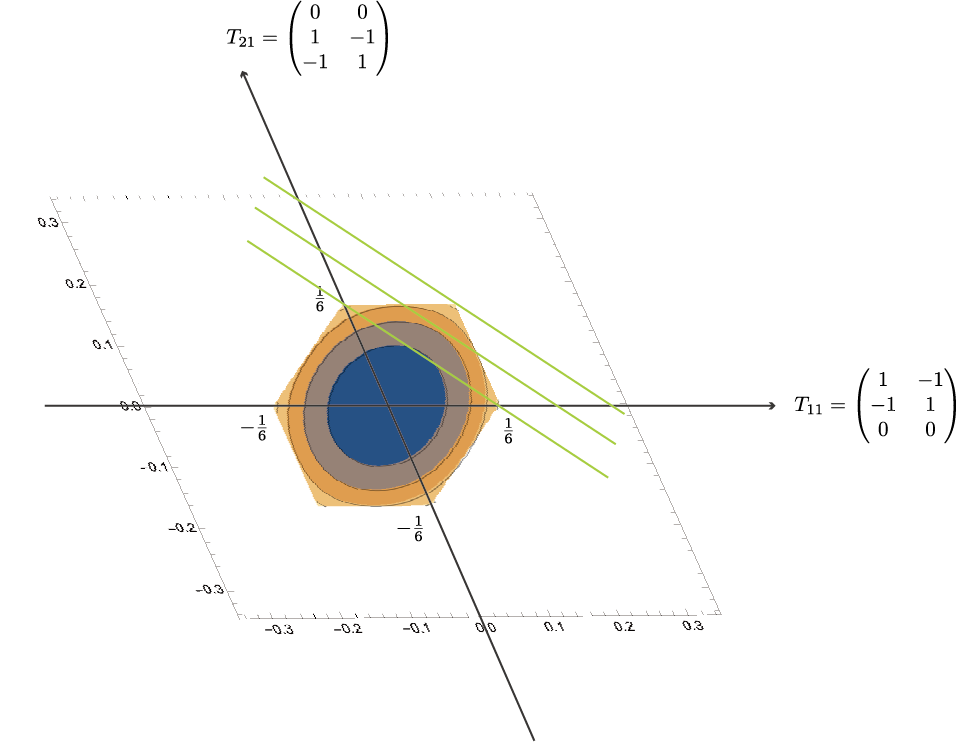
Fig. 1: Visualization of $3\times 2$ checkerboard copulas space. The irregular hexagon in the figure represents the domain of a checkerboard copula. Ovals inside it represents the contour lines of the information of copulas. The line corresponds to a region where Kendall’s $\tau$ remains constant.

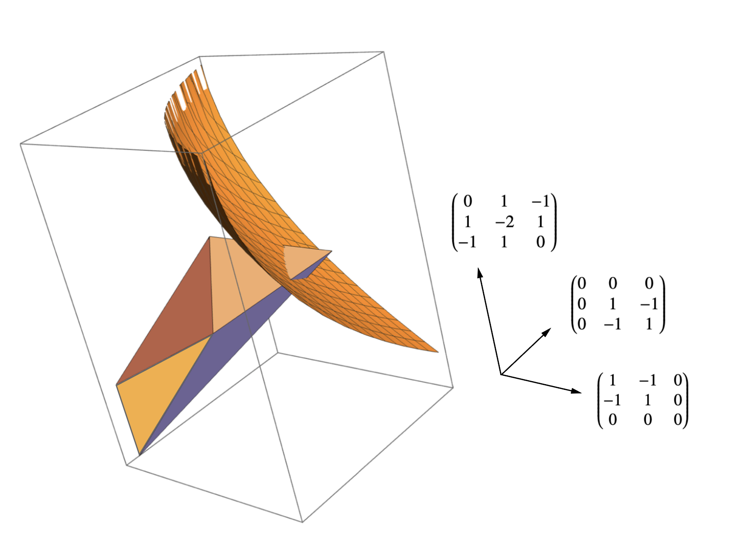
Fig. 2: Visualization of $3\times 3$ checkerboard copulas space. The polyhedron in the figure represents the domain of a checkerboard copula. The curved surface corresponds to a region where Kendall’s $\tau$ remains constant.

Example 7 ($3\times 3$ checkerboard copulas).

Expression of a copula $P$ in new coordinates is

$$P=\begin{pmatrix}p_{11}&p_{12}&p_{13}\\ p_{21}&p_{22}&p_{23}\\ p_{31}&p_{32}&p_{33}\end{pmatrix}=\begin{pmatrix}\frac{1}{9}&\frac{1}{9}&\frac{1}{9}\\ \frac{1}{9}&\frac{1}{9}&\frac{1}{9}\\ \frac{1}{9}&\frac{1}{9}&\frac{1}{9}\end{pmatrix} +p^{\prime}_{11}\begin{pmatrix}1&-1&0\\ -1&1&0\\ 0&0&0\end{pmatrix}$$

$$+p^{\prime}_{21}\begin{pmatrix}0&0&0\\ 1&-1&0\\ -1&1&0\end{pmatrix}+p^{\prime}_{12}\begin{pmatrix}0&1&-1\\ 0&-1&1\\ 0&0&0\end{pmatrix}+p^{\prime}_{22}\begin{pmatrix}0&0&0\\ 0&1&-1\\ 0&-1&1\end{pmatrix}.$$

The degree of freedom is four. To reduce its dimension so that it can be visualized in the 3 dimensional space, we assume symmetric matrices here temporarily, i.e., $p_{12}=p_{21}$. Then, we have

$$P=\begin{pmatrix}p_{11}&p_{12}&p_{13}\\ p_{21}&p_{22}&p_{23}\\ p_{31}&p_{32}&p_{33}\end{pmatrix}=\begin{pmatrix}\frac{1}{9}&\frac{1}{9}&\frac{1}{9}\\ \frac{1}{9}&\frac{1}{9}&\frac{1}{9}\\ \frac{1}{9}&\frac{1}{9}&\frac{1}{9}\end{pmatrix}+p^{\prime}_{11}\begin{pmatrix}1&-1&0\\ -1&1&0\\ 0&0&0\end{pmatrix}+p^{\prime}_{12}\begin{pmatrix}0&1&-1\\ 1&-2&1\\ -1&1&0\end{pmatrix}+p^{\prime}_{22}\begin{pmatrix}0&0&0\\ 0&1&-1\\ 0&-1&1\end{pmatrix}.$$

The constraint on Kendall’s tau (3) becomes

$$2p^{\prime}_{11}p^{\prime}_{22}-2p^{\prime 2}_{12}+\frac{8}{9}(p^{\prime}_{11}+p^{\prime}_{22}+2p^{\prime}_{12})=\mu.$$

3.3 Pseudo log odds ratio of MICK

Finally, we observe that a certain local dependence of MICK is constant everywhere. For every $2\times 2$ submatrices of the matrix associated with MICK, we state that the variant of well-known odds ratio always takes a constant value. This is derived by considering the stationary conditions for the problem $(\mathrm{P})$.

Lemma 1 (Variation of Kendall’s tau).

Let $\Pi=(\pi_{i,j})$ be a checkerboard copula. Consider a small change $\epsilon T_{ij}(\epsilon\ll 1)$ on $\Pi$. The variation of Kendall’s tau is

$$2\epsilon(\pi_{i,j}+\pi_{i+1,j+1}+\pi_{i+1,j}+\pi_{i,j+1})+O(\epsilon^{2})$$

This value $\pi_{i,j}+\pi_{i+1,j+1}+\pi_{i+1,j}+\pi_{i,j+1}$ is positive, meaning that Kendall’s tau always increases when $T_{ij}$ is added to a copula.

Proof of Lemma 1:.

$$t_{ij}^{\top}Wp =(\sum_{k=1}^{n}\sum_{l=1}^{n}w_{n(i-1)+j,k}p_{kl})-(\sum_{k=1}^{n}\sum_{l=1}^{n}w_{n(i-1)+j+1,k}p_{kl})-(\sum_{k=1}^{n}\sum_{l=1}^{n}w_{ni+j,k}p_{kl})+(\sum_{k=1}^{n}\sum_{l=1}^{n}w_{ni+j+1,k}p_{kl})$$

$$=\sum_{k=1}^{n}\sum_{l=1}^{n}(w_{n(i-1)+j,k}-w_{n(i-1)+j+1,k}-w_{ni+j,k}+w_{ni+j+1,k})p_{kl}$$

$$=-p_{i,j}-p_{i,j+1}-p_{i+1,j}-p_{i+1,j+1}$$

Let $\tau_{\Pi}$ be Kendall’s tau of $\Pi$ and $\tau_{\Pi+\epsilon T_{ij}}$ be that of $\Pi+\epsilon T_{ij}$. It follows that

$$\tau_{\Pi+\epsilon T_{ij}}-\tau_{\Pi} =(1-(\pi+\epsilon t_{ij})^{\top}W(\pi+\epsilon t_{ij}))-(1-\pi^{\top}W\pi)$$

$$=\pi^{\top}W\pi-(\pi+\epsilon t_{ij})^{\top}W(\pi+\epsilon t_{ij})$$

$$=-2\epsilon t_{ij}^{\top}W\pi-\epsilon^{2}t_{ij}^{\top}Wt_{ij}$$

$$=2\epsilon(\pi_{i,j}+\pi_{i,j+1}+\pi_{i+1,j}+\pi_{i+1,j+1})+O(\epsilon^{2}).$$

∎

Lemma 2.

Assume $\epsilon\ll 1$. Let

$$\delta=\frac{\pi_{i,j}+\pi_{i+1,j}+\pi_{i+1,j}+\pi_{i+1,j+1}}{\pi_{i^{\prime},j^{\prime}}+\pi_{i^{\prime}+1,j^{\prime}}+\pi_{i^{\prime}+1,j^{\prime}}+\pi_{i^{\prime}+1,j^{\prime}+1}}\epsilon.$$

Then,

$$1-\mathrm{Tr}(\Xi\Pi\Xi\Pi^{\top})=1-\mathrm{Tr}(\Xi\Pi^{\prime}\Xi{\Pi^{\prime}}^{\top})+O(\epsilon^{2}),\ \Pi^{\prime}:=\Pi+\epsilon T_{ij}-\delta T_{i^{\prime}j^{\prime}}$$

This lemma states Kendall’s tau is invariant under the operation $\epsilon T_{ij}-\delta T_{i^{\prime}j^{\prime}}$. The proof is straightforward from Lemma 1.

Lemma 3 (Variation of the objective function).

Let $\Pi=(\pi_{i,j})$ be a checkerboard copula. Consider a small change $\epsilon T_{ij}(\epsilon\ll 1)$ on $\Pi$. The variation of copula information is

$$\epsilon\log{\frac{\pi_{i,j}\pi_{i+1,j+1}}{\pi_{i+1,j}\pi_{i,j+1}}}.$$

Proof of Lemma 3.

$$\frac{\partial}{\partial\pi_{ij}}(\sum_{i}\sum_{j}\pi_{ij}\log{\pi_{ij}})=\log{\pi_{ij}}+1,$$

so the increase in the information of $\Pi$ by the operation $\epsilon T_{ij}$ is

$$\epsilon(\log{\pi_{ij}}+1)+\epsilon(\log{\pi_{i+1,j+1}}+1)-\epsilon(\log{\pi_{i+1,j}}+1)-\epsilon(\log{\pi_{i,j+1}}+1)=\epsilon\log{\frac{\pi_{i,j}\pi_{i+1,j+1}}{\pi_{i+1,j}\pi_{i,j+1}}}.$$

∎

Two variations from Lemma 1 and Lemma 3 lead to the following main statement.

Theorem 3.

The following value is constant for every $2\times 2$ submatrices $\begin{pmatrix}\pi_{i,j}&\pi_{i,j+1}\\ \pi_{i+1,j}&\pi_{i+1,j+1}\\ \end{pmatrix}$ on MICK.

$$\frac{1}{\pi_{i,j}+\pi_{i+1,j}+\pi_{i+1,j}+\pi_{i+1,j+1}}\log{\frac{\pi_{i,j}\pi_{i+1,j+1}}{\pi_{i+1,j}\pi_{i,j+1}}}$$

We name this common value “pseudo log odds ratio”.

Proof of Theorem 3.

The stationary condition for the optimization problem $(P)$ is

$$\forall\epsilon(\ll 1),i,j,i^{\prime},j^{\prime},\epsilon\log{\frac{\pi_{i,j}\pi_{i+1,j+1}}{\pi_{i+1,j}\pi_{i,j+1}}}-\delta\log{\frac{\pi_{i^{\prime},j^{\prime}}\pi_{i^{\prime}+1,j^{\prime}+1}}{\pi_{i^{\prime}+1,j^{\prime}}\pi_{i^{\prime},j^{\prime}+1}}}=0$$

Therefore, we obtain

$$\frac{\pi_{i^{\prime},j^{\prime}}+\pi_{i^{\prime}+1,j^{\prime}}+\pi_{i^{\prime}+1,j^{\prime}}+\pi_{i^{\prime}+1,j^{\prime}+1}}{\pi_{i,j}+\pi_{i+1,j}+\pi_{i+1,j}+\pi_{i+1,j+1}}\log{\frac{\pi_{i,j}\pi_{i+1,j+1}}{\pi_{i+1,j}\pi_{i,j+1}}}-\log{\frac{\pi_{i^{\prime},j^{\prime}}\pi_{i^{\prime}+1,j^{\prime}+1}}{\pi_{i^{\prime}+1,j^{\prime}}\pi_{i^{\prime},j^{\prime}+1}}}=0$$

$$\Leftrightarrow\frac{1}{\pi_{i,j}+\pi_{i+1,j}+\pi_{i+1,j}+\pi_{i+1,j+1}}\log{\frac{\pi_{i,j}\pi_{i+1,j+1}}{\pi_{i+1,j}\pi_{i,j+1}}}=\frac{1}{\pi_{i^{\prime},j^{\prime}}+\pi_{i^{\prime}+1,j^{\prime}}+\pi_{i^{\prime}+1,j^{\prime}}+\pi_{i^{\prime}+1,j^{\prime}+1}}\log{\frac{\pi_{i^{\prime},j^{\prime}}\pi_{i^{\prime}+1,j^{\prime}+1}}{\pi_{i^{\prime}+1,j^{\prime}}\pi_{i^{\prime},j^{\prime}+1}}}.$$

Note that both sides of the equation has the same form for $(i,j)$ and $(i^{\prime},j^{\prime})$. ∎

Another proof through Lagrangian method will be provided in Appendix A. The understanding of “pseudo log odds ratio” will be provided in Section 4 along with the comparison between MICK and MICS.

From Theorem 3, it is direct that the density function of MICK has a preferable positive dependence property known as “total positivity”. A function is said to be TP2 (short for “total positivity of order two”) when $f(x,y)f(x^{\prime},y^{\prime})\geq f(x,y^{\prime})f(x^{\prime},y)$ for any pairs $(x,y)$ and $(x^{\prime},y^{\prime})$, where $x<x^{\prime}$ and $y<y^{\prime}$ [4]. If $f(x,y)$ is a joint density, $f(x,y)$ is said to be d-TP2 (short for density TP2), which is the strongest notion of positive dependence – stronger than TP2 and also stronger than stochastic increasingness (SI) [4]. d-TP2 is also referred to as “positively likelihood ratio dependence” [9].

Theorem 4.

MICK belongs to d-TP2.

Proof.

Assuming the entries of checkerboard copula is all strictly positive, $\log{\frac{\pi_{i,j}\pi_{i+1,j+1}}{\pi_{i+1,j}\pi_{i,j+1}}}>0$ is equivalent to $\pi_{i,j}\pi_{i+1,j+1}>\pi_{i+1,j}\pi_{i,j+1}\Leftrightarrow\mathrm{det}\begin{pmatrix}\pi_{i,j}&\pi_{i,j+1}\\ \pi_{i+1,j}&\pi_{i+1,j+1}\\ \end{pmatrix}>0$. ∎

As Theorem 3 only states the sufficient condition of the optimal solution of $(\mathrm{P})$, we are naturally interested in the uniqueness of it. As our main result, we state that when the given Kendall’s rank correlation (or the corresponding pseudo log odds ratio) is small enough, the optimal solution becomes unique despite the non-convexity of the problem.

Theorem 5.

The optimization problem $(\mathrm{P})$ has a unique optimal solution when $\lambda<2$. This corresponds to the condition that pseudo log odds ratio of MICK is smaller than 4.

The proof follows by considering the information on an arbitrary curve passing through a stationary point and calculating the Hessian there. Local convexity of the information on every stationary points leads to the statement. The complete proof is given in Appendix B.

3.4 Numerical calculation

To utilize MICK for real data analysis, one needs to be able to compute it numerically. One naive approach is to use numerical solvers to directly obtain optimal solutions for $(\mathrm{P})$, or $(\mathrm{RP})$ since the solutions are identical as mentioned before. However, computational limitations become problematic. Empirically, it is difficult to reach the optimal solution due to the iteration limit when the gridsize $n$ is larger than 10. Instead, we can take advantage of the results in Theorem 3. We have already confirmed that pseudo log odds ratio is constant on MICK, thus the numerical solution is obtained as follows:

Algorithm 1 Greedy calculation of MICK

0:  pseudo log odds ratio $r$

1:  $M\leftarrow n\times n$ uniform copula

2:  while converge do

3:     Choose a $2\times 2$ submatrix $\begin{pmatrix}\pi_{i,j}&\pi_{i,j+1}\\ \pi_{i+1,j}&\pi_{i+1,j+1}\\ \end{pmatrix}$ of $M$.

4:     Solve

$$\frac{1}{\pi_{ij}+\pi_{i+1,j}+\pi_{i,j+1}+\pi_{i+1,j+1}}\log{\frac{(\pi_{i,j}+\delta)(\pi_{i+1,j+1}+\delta)}{(\pi_{i+1,j}-\delta)(\pi_{i,j+1}-\delta)}}=r$$

5:     Update $\begin{pmatrix}\pi_{i,j}&\pi_{i,j+1}\\ \pi_{i+1,j}&\pi_{i+1,j+1}\\ \end{pmatrix}\to\begin{pmatrix}\pi_{i,j}+\delta&\pi_{i,j+1}-\delta\\ \pi_{i+1,j}-\delta&\pi_{i+1,j+1}+\delta\\ \end{pmatrix}$

6:  end while

Note that the procedure 4 is to just solve a quadratic equation w.r.t. $\delta$ and thus computationally efficient. Figure 3 shows the obtained MICK. Note that the algorithm requires in advance the value of pseudo log odds ratio instead of the rank correlation. The explicit relationship between these two is unknown, however, it is possible to numerically specify the appropriate value of log odds ratio by binary search, due to its monotonicity. See Appendix C for more details.

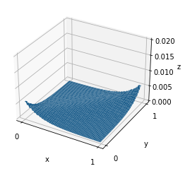
Fig. 3: MICK, $n=30$, $\mu=0.5$, pseudo log odds ratio = 2.9

4 On the comparison between MICK and MICS

We end this paper with a discussion aimed at comparing parallel stories between MICK and MICS.

4.1 Theoretical perspective

Let us review the optimization problem for MICS mentioned in Example 3.

$$\mathrm{minimize}\ \sum_{i=1}^{I}\sum_{j=1}^{J}\pi_{ij}\log{\pi_{ij}}$$

$$\mathrm{s.t.}\ \sum_{i=1}^{I}\pi_{ij}=\frac{1}{J},\ \sum_{j=1}^{J}\pi_{ij}=\frac{1}{I},$$

$$0\leq\pi_{ij}\leq 1,$$

$$\sum_{i=1}^{n}\sum_{j=1}^{n}h_{ij}\pi_{ij}=\mu,\ \mathrm{where}\ h_{ij}=12(i-\frac{1}{2})(j-\frac{1}{2}).$$

The only difference in the problem settings for MICK and MICS is its final constraint. However, this difference is not trivial because the latter becomes a convex programming due to the linearity of Spearman’s $\rho$. Therefore, MICS exists uniquely and has the form of $p_{ij}=A_{i}B_{j}\exp{(\theta h_{ij})}$, where $h_{ij}=12(i-\frac{1}{2})(j-\frac{1}{2})$ corresponds to Spearman’s $\rho$. From information geometric perspective, one-to-one correspondence is also known for $\theta$ and $\mu$. This means MICS is specified by the parameter $\mu$ from its definition, it can also be specified by the parameter $\theta$ instead, i.e., MICS forms a one-parameter-family $\{A_{i}B_{j}\exp{(\theta h_{ij})}\ |\ \theta\in\mathbb{R}\}$. These facts follow from the more general statements in previous researches [1] [17].

Following the similar argument for MICK in Section 3, it leads to the statement that log odds ratio $\log{\frac{p_{i,j}p_{i+1,j+1}}{p_{i+1,j}p_{i,j+1}}}$ is constant everywhere in MICS due to the fact that the variance of Spearman’s rho by $T_{ij}$ becomes constant for any $(i,j)$. Indeed, this result is obvious because it is already known in the previous works that the actual form of MICS is

$$p_{ij}=A_{i}B_{j}\exp{(\theta h_{ij})}=A_{i}B_{j}\exp{\left(12\theta(i-\frac{1}{2})(j-\frac{1}{2})\right)}.$$

Although we do not have the explicit form of the regularization factors $A_{i}$ and $B_{j}$, it cancels out during the direct calculation, which leads to

$$\log{\frac{p_{i,j}p_{i+1,j+1}}{p_{i+1,j}p_{i,j+1}}}=\theta.$$ (7)

As is mentioned previously, $\theta$ is an important constant that specifies the distribution of MICS completely.

We further make a first step to analyze tail dependence of minimum information copulas in a continuous problem setting. This is because the tail dependence coefficient of checkerboard copulas always results in zero. See Theorem 17 in Durrleman et al. [3] Due to the regularization terms, even the tail dependence of MICS has been unclear. We provide a partial result assuming that the resulting minimum information copula is close enough to the uniform copula, implying that MICK has a heavier tail dependence than MICS.

Theorem 6.

Suppose continuous version of MICK and MICS have the same value of Lagrangian multiplier $\lambda\ (|\lambda|\ll 1)$. Further assume both of them are close enough to the uniform copula and consider their expansions w.r.t. $\lambda$:

$$p(x,y)=1+\lambda q(x,y)+\lambda^{2}r(x,y)+o(\lambda^{2}).$$

Then,

$$q(x,y)\to\frac{1}{4},r(x,y)\to\frac{1}{48}$$

for MICK and

$$q(x,y)\to\frac{1}{4},r(x,y)\to\frac{1}{72}$$

for MICS when $(x,y)\to(0,0)$.

As a result, the parallel theoretical properties of MICK and MICS are summarized as in Table 1. A natural question arises as to whether MICK is uniquely specified by the pseudo log odds ratio, similar to MICS being specified by log odds ratio. The solution to this is partially given previously in Theorem 5. In other words, both $n\times n$ MICK and $n\times n$ MICS are determined by the set of local dependence with the size of $(n-1)^{2}$. Comparing these two notions, the difference comes from the term $p_{ij}+p_{i+1,j+1}+p_{i+1,j}+p_{i,j+1}$, i.e., the sum of probability mass on four grids of the checkerboard copula. This observation can be interpreted in terms of odds ratio as follows: MICK put more weights on regions with higher odds ratio, while MICS put uniform weights on every region of a checkerboard copula.

Table 1: Comparison between MICK and MICS

	MICK	MICS
constraint	Kendall’s $\tau$	Spearman’s $\rho$
convexity	non-convex	convex
checkerboard copula $p_{ij}$	not known	$p_{ij}=A_{i}B_{j}\exp{\left(12\theta(i-\frac{1}{2})(j-\frac{1}{2})\right)}$
dependence	TP2	TP$\infty$
constant value	pseudo log odds ratio $\frac{1}{p_{ij}+p_{i+1,j+1}+p_{i+1,j}+p_{i,j+1}}\log{\frac{p_{ij}p_{i+1,j+1}}{p_{i+1,j}p_{i,j+1}}}=2\lambda^{MICK}$	log odds ratio $\log{\frac{p_{ij}p_{i+1,j+1}}{p_{i+1,j}p_{i,j+1}}}=\frac{1}{n^{2}}\lambda^{MICS}=\theta$
density on tails (See Theorem 6.)	$p(x,y)=1+\frac{\lambda}{4}+\frac{\lambda^{2}}{48}$	$p(x,y)=1+\frac{\lambda}{4}+\frac{\lambda^{2}}{72}$

4.2 Fitting to financial data

MICK and MICS can be used in the context of uncertainty modeling, where inadequate information on the true distribution is accessible. Uncertainty distributions need to be specified either by fitting to data or by expert judgement. Using MICK or MICS enables us to extract information exclusively from rank correlation of the given data. In this section, we demonstrate a plausible way to fit MICK and MICS to real data. We use daily stock price datasets, Dow Jones Average and S&P 500, as observed data as an example. All data were collected from Pandas-Datareader. First, data are preprocessed into order rank statistics of log return. Then, the sample version of rank correlations are calculated from observed data. Finally, we obtain MICK/MICS following Algorithm 1.

Following Sei [17], data preprocessing was conducted in the following way in order to transfer the domain into $[0,1]\times[0,1]$ before modelling with a copula. Let $n$ be the number of data. For observed data $(x_{i},y_{i})_{i=1,\dots,n}$,

1. Calculate the order rank $r_{x},r_{y}$ of each record,

2. $x_{i}\leftarrow\frac{1}{n}r_{x},$

3. $y_{i}\leftarrow\frac{1}{n}r_{y}.$

The overview of data is shown in Figure 4 and Figure 5. Data length was 1635. Preprocessed data are depicted in Figure 6. The important statistics used in this section are the sample Kendall’s tau $\tau$, the sample Spearman’s rho $\rho$, estimated lower tail dependence $\lambda_{L}^{u\%}=\mathrm{Pr}[F_{2}(X_{2})<u/100|F_{1}(X_{1})<u/100]\ (u=1,5)$, and estimated upper tail dependence $\lambda_{U}^{u\%}=\mathrm{Pr}[F_{2}(X_{2})>(100-u)/100|F_{1}(X_{1})>(100-u)/100]\ (u=1,5)$. The original data have

$$(\tau^{\mathrm{obs}},\rho^{\mathrm{obs}},\lambda_{L}^{5\%,{\mathrm{obs}}},\lambda_{U}^{5\%,{\mathrm{obs}}},\lambda_{L}^{1\%,{\mathrm{obs}}},\lambda_{U}^{1\%,{\mathrm{obs}}})=(0.802,0.939,0.827,0.753,0.812,0.937).$$

Note that preprocessing does not affect these statistics.

Fig. 4: log return of Dow Jones Average and S&P 500

Fig. 5: log return of Dow Jones Average vs S&P 500

Fig. 6: log return of Dow Jones Average vs S&P 500 (preprocessed)

Using the numerical obtained MICK and MICS, we simulated data from financial data to evaluate the performance of MICK. To simulate these plots, we first decide $\mu$ in $(P)$ empirically as well as method of moments. In this case, $\mu=\tau^{\mathrm{obs}}=0.802$. Figure 8 shows the simulated plots. The gridsize of MICK is set to $30\times 30$. The mean of 1000 runs were

$$(\tau,\rho,\lambda_{L}^{5\%},\lambda_{U}^{5\%},\lambda_{L}^{1\%},\lambda_{U}^{1\%})=(0.801,0.949,0.467,0.471,0.112,0.115).$$

We also fit MICS for comparison as well. In this case, $\mu=\rho^{\mathrm{obs}}=0.939$. The gridsize of MICK is set to $30\times 30$. Figure 8 shows the simulated plots. The mean of 1000 runs were

$$(\tau,\rho,\lambda_{L}^{5\%},\lambda_{U}^{5\%},\lambda_{L}^{1\%},\lambda_{U}^{1\%})=(0.774,0.939,0.367,0.369,0.086,0.086).$$

This result implies MICK is more capable of capturing tail dependences than MICS.

Fig. 7: Simulation scattering of MICK ($\tau=0.802$)

Fig. 8: Simulation scattering of MICS ($\rho=0.909$)

Table 2: The statistics of observed and simulated data

	Observed	Simulated MICK	Simulated MICS
$\tau$	0.802	0.801	0.774
$\rho$	0.939	0.949	0.939
$\lambda_{L}^{5\%}$	0.827	0.467	0.367
$\lambda_{U}^{5\%}$	0.753	0.471	0.369
$\lambda_{L}^{1\%}$	0.812	0.112	0.086
$\lambda_{U}^{1\%}$	0.937	0.115	0.086

4.3 Relationship with Optimal Transport

Finally, we point out the relationship between discrete version of minimum information copula and entropic optimal transport problem additionally.

In some articles, the equivalency between the minimum information copula and the optimal transport problem is mentioned [17]. More specifically, the optimization problem for a minimum information copula is known to be equivalent to the optimal transport problem with entropy regularization. In fact, both Lagrangian coincides:

$$\mathcal{L}(\Pi,\alpha,\beta)=\sum_{i=1}^{n}\sum_{j=1}^{n}(D_{ij}\pi_{ij})+\frac{1}{\lambda}\sum_{i=1}^{n}\sum_{j=1}^{n}(\pi_{ij}\log{\pi_{ij}}-\pi_{ij})+\sum_{i=1}^{n}\alpha_{i}([\Pi 1_{n}]_{i}-\frac{1}{n})+\sum_{j=1}^{n}\beta_{j}([\Pi^{\top}1_{n}]_{j}-\frac{1}{n}),$$

where $\alpha\in\mathbb{R}^{n}$ and $\beta\in\mathbb{R}^{n}$ are the Lagrangian multipliers and $D_{ij}$ represents the cost of the transport from $i$ to $j$. MICS is also included in this case.

Analogously, the optimization problem (P) for MICK can also be interpreted as a new variant of optimal transport with entropy regularization controlled by parameter $\frac{1}{\lambda}$:

$$\min\ 1-\sum_{i=1}^{n}\sum_{j=1}^{n}\sum_{p=1}^{n}\sum_{q=1}^{n}\pi_{ij}\pi_{pq}\xi_{ip}\xi_{qj}+\frac{1}{\lambda}\sum_{i=1}^{n}\sum_{j=1}^{n}(\pi_{ij}\log{\pi_{ij}}-\pi_{ij})$$

$$=\sum_{i=1}^{n}\sum_{j=1}^{n}\sum_{p=1}^{n}\sum_{q=1}^{n}\pi_{ij}\pi_{pq}v_{ijpq}+\frac{1}{\lambda}\sum_{i=1}^{n}\sum_{j=1}^{n}(\pi_{ij}\log{\pi_{ij}}-\pi_{ij}),$$

$$\mathrm{s.t.}\ \sum_{i=1}^{n}\pi_{ij}=\frac{1}{n},\sum_{j=1}^{n}\pi_{ij}=\frac{1}{n},$$

with its Lagrangian being

$$\mathcal{L} =1-\sum_{i=1}^{n}\sum_{j=1}^{n}\sum_{p=1}^{n}\sum_{q=1}^{n}\pi_{ij}\pi_{pq}\xi_{ip}\xi_{qj}+\frac{1}{\lambda}\sum_{i=1}^{n}\sum_{j=1}^{n}(\pi_{ij}\log{\pi_{ij}}-\pi_{ij})+\sum_{i=1}^{n}\alpha_{i}([\Pi 1_{n}]_{i}-\frac{1}{n})+\sum_{j=1}^{n}\beta_{j}([\Pi^{\top}1_{n}]_{j}-\frac{1}{n}).$$

As well as usual optimal transport problems, this problem can be interpreted as a bipartite graph matching: Let $G=(U\cup V,E)$ be a bipartite graph with $n^{2}$ transport edges, where $|U|=|V|=n$. Pick any couple of two edges. The cost $v_{ijpq}=-(\xi_{ip}-1)(\xi_{qj}-1)$ becomes $+1$ when the two edges $i\to j$ and $p\to q$ intersect, $0$ if either start or goal of two edges coincides, and $-1$ otherwise. The amount of mass is calculated as the multiplication of two transported masses. Here, we want to minimize the summation of each mass multiplied by each associated cost.

5 Discussion

There has been an increasing interest in copula entropy theories as a solution to misspecification issue [1]. The concept of maximizing entropy corresponds to minimum information copulas since the famous Shannon entropy and information are closely linked. In this paper, we formulated a minimum information checkerboard copula under fixed Kendall’s rank correlation and named it MICK.

MICK is originally defined as the optimal solution of a non-convex programming. We confirmed that it can also be characterised in another way by the variant of odds ratio. This result implies the global dependence is determined by the series of the local dependence. Taking advantage of this property, we constructed a quick algorithm to obtain MICK numerically even with a large grid size, enabling us to apply it to real data analysis.

Since the concept of MICK is simplified, the extension of MICK is straightforward. First, the constraints to specify the copula density could be more general. In recent works, the expectation of a certain function, such as moments of the distribution, was only assumed as the constraints. We extended this to a second-order constraint in this work. Specifically, we focused on a single constraint that fixes Kendall’s $\tau$ and also made a comparison with another important notion, Spearman’s $\rho$. Recently, statistical notions that measure the dependence between multiple random variables in various domains, such as distance correlation. Extending the results to these is a future work of interest.

Furthermore, applying MICK to higher dimensions is of great interest. We developed MICK only for bivariate checkerboard copula in this paper. However, the results can be applied to three or more variables since the notion of information and Kendall’s $\tau$ are not specific to bivariate cases. In three dimensional case for example, the given constraint should be fixing Kendall’s $\tau$ for the trivariate checkerboard copula $P$: $p^{\top}(V\otimes V\otimes V)p$.

Last but not least, other than Shannon entropy considered in this paper, Tsallis entropy and Renyi entropy should also be discussed. It is possible that Tsallis entropy associated with power-law distribution naturally leads to copulas with heavier tail dependence, which is preferable for risk analysis in finance.

Appendix A. Another proof for Theorem 3.

Here, we view that Theorem 3 coincides with the Lagrangian method applied after the coordinate transformation introduced in Section 3.2. By applying the transformation in (5) and (6), the main problem (P) can be rewritten as follows:

$$\min\sum_{i}\sum_{j}\{((A\otimes A)p^{\prime})_{ij}+\frac{1}{n^{2}}\}\log\{((A\otimes A)p^{\prime})_{ij}+\frac{1}{n^{2}}\},$$

$$\mathrm{s.t.}\ p^{\prime}{{}^{\top}}(A\otimes A)^{\top}W(A\otimes A)p^{\prime}+\frac{2}{n^{2}}1^{\top}W(A\otimes A)p^{\prime}+\mu=0.$$

Let $\mathcal{L}$ denote the Lagrangian of this optimization problem. Then, it is recovered from its stationary condition that the pseudo log odds ratio is constant:

$$\mathcal{L}=\sum_{i}\sum_{j}\{((A\otimes A)p^{\prime})_{ij}+\frac{1}{n^{2}}\}\log\{((A\otimes A)p^{\prime})_{ij}+\frac{1}{n^{2}}\}+\lambda\{p^{\prime}{{}^{\top}}(A\otimes A)^{\top}W(A\otimes A)p^{\prime}+\frac{2}{n^{2}}1_{n^{2}}^{\top}W(A\otimes A)p^{\prime}+\mu\},$$

$$\lambda>0.$$

Hence,

$$\frac{\partial\mathcal{L}}{\partial p^{\prime}_{ij}} =\frac{\partial}{\partial p^{\prime}_{ij}}(p_{ij}\log{p_{ij}}+p_{i+1,j}\log{p_{i+1,j}}+p_{i,j+1}\log{p_{i,j+1}}+p_{i+1,j+1}\log{p_{i+1,j+1}}$$

$$+\lambda\{p^{\prime}{{}^{\top}}(A\otimes A)^{\top}W(A\otimes A)p^{\prime}+\frac{2}{n^{2}}1_{n^{2}}^{\top}W(A\otimes A)p^{\prime}+\mu\})$$

$$=\frac{\partial p_{ij}}{\partial p^{\prime}_{ij}}(\log{p_{ij}}+1)+\frac{\partial p_{i+1,j}}{\partial p^{\prime}_{ij}}(\log{p_{i+1,j}}+1)+\frac{\partial p_{i,j+1}}{\partial p^{\prime}_{ij}}(\log{p_{i,j+1}}+1)+\frac{\partial p_{i+1,j+1}}{\partial p^{\prime}_{ij}}(\log{p_{i+1,j}}+1)$$

$$+\lambda\{2((A\otimes A)^{\top}W(A\otimes A)p^{\prime})_{ij}+\frac{2}{n^{2}}((A\otimes A)^{\top}W1_{n^{2}})_{ij}\}$$

$$=\log{\frac{p_{ij}p_{i+1,j+1}}{p_{i+1,j}p_{i,j+1}}}+\lambda\{2(-p_{ij}-p_{i+1,j}-p_{i,j+1}-p_{i+1,j+1}+\frac{4}{n^{2}})-\frac{8}{n^{2}}\}$$

$$=\log{\frac{p_{ij}p_{i+1,j+1}}{p_{i+1,j}p_{i,j+1}}}-2\lambda(p_{ij}+p_{i+1,j}+p_{i,j+1}+p_{i+1,j+1}).$$

Therefore, we obtain the stationary condition:

$$\frac{\partial\mathcal{L}}{\partial p^{\prime}_{ij}} =0\Leftrightarrow 2\lambda=\frac{1}{p_{ij}+p_{i+1,j+1}+p_{i+1,j}+p_{i,j+1}}\log{\frac{p_{ij}p_{i+1,j+1}}{p_{i+1,j}p_{i,j+1}}}.$$ (8)

Since the problem settings are parallel between MICK and MICS, we are able to derive the stationary condition that MICS satisfies, as well. After the basis transformation as in Section 4.4, the optimization problem for MICS becomes

$$\min\sum_{i}\sum_{j}\{((A\otimes A)p^{\prime})_{ij}+\frac{1}{n^{2}}\}\log\{((A\otimes A)p^{\prime})_{ij}+\frac{1}{n^{2}}\},$$

$$\mathrm{s.t.}\ \bar{w}^{\top}(A\otimes A)p^{\prime}=\frac{\mu}{12},$$

where $\bar{w}$ is a vector aligning every entries of $W^{\top}$ in one row. Lagrangian of this problem is

$$\mathcal{L}=\{((A\otimes A)p^{\prime})_{ij}+\frac{1}{n^{2}}\}\log\{((A\otimes A)p^{\prime})_{ij}+\frac{1}{n^{2}}\}-\lambda\left(\bar{w}^{\top}(A\otimes A)p^{\prime}-\frac{\mu}{12}\right)$$

$$\frac{\partial\mathcal{L}}{\partial p^{\prime}_{ij}}=\log{\frac{p_{ij}p_{i+1,j+1}}{p_{i+1,j}p_{i,j+1}}}-\lambda((A\otimes A)^{\top}\bar{w})_{(n-1)(i-1)+j}$$

$$\frac{\partial\mathcal{L}}{\partial p^{\prime}_{ij}}=0\Leftrightarrow\frac{\partial\mathcal{L}}{\partial p^{\prime}_{ij}}=\log{\frac{p_{i,j}p_{i+1,j+1}}{p_{i+1,j}p_{i,j+1}}-\frac{\lambda}{n^{2}}}.$$

Thus, its stationary condition is

$$\frac{\lambda}{n^{2}}=\log{\frac{p_{i,j}p_{i+1,j+1}}{p_{i+1,j}p_{i,j+1}}}.$$

Appendix B. Proof for Theorem 5.

Proof for Theorem 5..

Let $P_{0}$ be an optimal solution of $(\mathrm{P})$ and $P_{t}$ be a curve parameterized by $t\ (\in\mathbb{R})$ with a constant Kendall’s $\tau$. Since Kendall’s $\tau$ is written as $\tau=1-\mathrm{tr}(P\Xi P\Xi^{\top})=1-p^{\top}Wp$, $p_{t}$ satisfies the followings:

$$p_{t}^{\top}Wp_{t}=const.$$

$${p^{\prime}_{t}}^{\top}Wp_{t}=0.$$

$${p^{\prime\prime}_{t}}^{\top}Wp_{t}+{p^{\prime}_{t}}^{\top}Wp^{\prime}_{t}=0,$$

where $p^{\prime}_{t}$ and $p^{\prime\prime}_{t}$ are first and second derivative of $p_{t}$ w.r.t. $t$, respectively. The objective function $F$ along this curve is

$$F_{t}=\sum_{i}\sum_{j}P_{t,ij}\log{P_{t,ij}}.$$

By taking derivatives with respect to the parameter $t$,

$$F^{\prime}_{t}=\sum_{i}\sum_{j}P^{\prime}_{t,ij}(\log{P_{t,ij}}+1),$$

$$F^{\prime\prime}_{t}=\sum_{i}\sum_{j}{P^{\prime\prime}}_{t,ij}(\log{P_{t,ij}}+1)+\frac{{P^{\prime}}_{t,ij}^{2}}{P_{t,ij}}.$$

Since $P_{0}$ is the optimal solution, $P_{0}$ should satisfy the following stationary condition.

$$\mathcal{L}=\sum_{i=1}^{I}\sum_{j=1}^{J}P_{ij}\log{P_{ij}}+\lambda(1-\mathrm{tr}(\Xi P\Xi P^{\top})-\mu)+\sum\alpha_{j}(\sum_{i=1}^{I}P_{ij}-\frac{1}{J})+\sum\beta_{i}(\sum_{j=1}^{J}P_{ij}-\frac{1}{I})$$

$$\frac{\partial\mathcal{L}}{\partial P_{ij}}=\log{P_{ij}}-\lambda(Wp)_{ij}+\alpha_{j}+\beta_{i}=0$$

Therefore, with $t=0$,

$$F^{\prime\prime}_{t}=\sum_{i}\sum_{j}{P^{\prime\prime}}_{t,ij}\lambda(Wp_{t})_{n(i-1)+j}+\sum_{i}\sum_{j}{P^{\prime\prime}}_{t,ij}(1-\alpha_{j}-\beta_{i})+\sum_{i}\sum_{j}\frac{{P^{\prime}}_{t,ij}^{2}}{P_{t,ij}}$$

For any $t$, row sum and column sum are constants:$\sum_{i}P_{ij}=\frac{1}{J},\sum_{j}P_{ij}=\frac{1}{I}$. Hence, by taking derivatives with $t$, $\sum_{i}{{P^{\prime\prime}}_{t}}_{ij}=0,\sum_{j}{{P^{\prime\prime}}_{t}}_{ij}=0.$

$$F^{\prime\prime}=\sum_{i}\sum_{j}\lambda({{p_{t}}^{\prime\prime}}_{n(i-1)+j}(Wp_{t})_{n(i-1)+j})+\sum_{i}\sum_{j}\frac{{P^{\prime}}_{t,ij}^{2}}{P_{t,ij}}$$

$$F^{\prime\prime}=\lambda{p_{t}}^{\prime\prime}Wp_{t}+{p_{t}}^{\prime}Diag(\frac{1}{p_{t,n(i-1)+j}}){p_{t}}^{\prime}$$

$$F^{\prime\prime}=-\lambda{p_{t}}^{\prime}W{p_{t}}^{\prime}+{p_{t}}^{\prime}Diag(\frac{1}{p_{t,ij}}){p_{t}}^{\prime}$$

$$F^{\prime\prime}={p_{t}}^{\prime}(Diag(\frac{1}{p_{t,ij}})-\lambda W){p_{t}}^{\prime}$$

Now, we consider changing the basis by

$$p=(A\otimes A)q+\frac{1}{n^{2}}1_{n^{2}},$$

where $p\in[0,\frac{1}{n}]^{n^{2}},q\in\mathbb{R}^{(n-1)^{2}}$. Then, by incorporating $q^{\prime}_{t}=(A\otimes A)p^{\prime}_{t}$, we have

$$F^{\prime\prime}=(q_{t}^{\prime})^{\top}(A\otimes A)^{\top}Diag(\frac{1}{p_{0,ij}})(A\otimes A)q_{t}^{\prime}-\lambda(q_{t}^{\prime})^{\top}(A\otimes A)^{\top}W(A\otimes A)q_{t}^{\prime}.$$

Define $D=(A\otimes A)^{\top}Diag(\frac{1}{p_{0,ij}})(A\otimes A)$ and $E=(A\otimes A)^{\top}W(A\otimes A)$. From tedious calculation, $E=-M\otimes M$. The problem is to examine whether $D-\lambda E$ is positive definite (PD). Here, we seek to obtain a constant $c$ such that

$$c\leq\min_{v,v^{\top}Ev>0}\frac{v^{\top}Dv}{v^{\top}Ev}.$$

With such $c$, it is easy to see that $\lambda<c\Rightarrow\forall v,v^{\top}Dv-\lambda v^{\top}Ev>0\Leftrightarrow(D-\lambda E)$ is PD.

Such a constant is obtained as the inverse of an upper bound of maximum eigenvalue due to the following argument:

$$\min_{v,v^{\top}Ev>0}\frac{v^{\top}Dv}{v^{\top}Ev} >\frac{1}{\max_{v,v^{\top}Ev>0}\frac{v^{\top}Ev}{v^{\top}Dv}}$$

$$>\frac{1}{\max_{v}\frac{v^{\top}Ev}{v^{\top}Dv}}$$

$$=\frac{1}{\max_{v}\frac{v^{\top}Ev}{v^{\top}LL^{\top}v}}$$

$$=\frac{1}{\max_{x,x=L^{\top}v}\frac{x^{\top}L^{\dagger}(-M\otimes M)(L^{\dagger})^{\top}x}{x^{\top}x}}$$

$$=\frac{1}{\lambda_{\max}(L^{\dagger}(-M\otimes M)(L^{\dagger})^{\top})},$$

where

$$L=(A\otimes A)^{\top}\mathrm{Diag}(\frac{1}{\sqrt{P_{0}}})$$

and

$$L^{\dagger}=\mathrm{Diag}(\sqrt{p_{0}})(A^{\dagger}\otimes A^{\dagger})^{\top}.$$

It can be confirmed that

$$LL^{\dagger}=E$$

and

$$LL^{\top}=(A\otimes A)^{\top}\mathrm{Diag}(\frac{1}{\sqrt{P_{0}}})\mathrm{Diag}(\frac{1}{\sqrt{P_{0}}})(A\otimes A)=(A\otimes A)^{\top}\mathrm{Diag}(\frac{1}{P_{0}})(A\otimes A)=D.$$

The last equation is due to the fact that $L^{\dagger}(-M\otimes M)(L^{\dagger})^{\top}$ is symmetric (Rayleigh quotient).

Now, the target matrix of interest can be transformed as follows:

$$L^{\dagger}(-M\otimes M)(L^{\dagger})^{\top} =\mathrm{Diag}(\sqrt{p_{0}})(A^{\dagger}\otimes A^{\dagger})^{\top}(-M\otimes M)(A^{\dagger}\otimes A^{\dagger})\mathrm{Diag}(\sqrt{p_{0}})$$

$$=-\mathrm{Diag}(\sqrt{p_{0}})(X\otimes X)\mathrm{Diag}(\sqrt{p_{0}}),$$

where $X=(A^{\dagger})^{\top}MA^{\dagger}$. The notion of $X$ differs between when $n$ is even and when $n$ is odd. Through tedious algebraic calculations, we have

$$X=\mathrm{Toeplitz}(-\frac{n-2}{n},-\frac{n-4}{n},\dots,\frac{n-2}{n},0,-\frac{n-2}{n},-\frac{n-4}{n},\dots,\frac{n-2}{n}),$$

$\mathrm{Diag}(\sqrt{p_{0}})(X\otimes X)\mathrm{Diag}(\sqrt{p_{0}})$ is a block matrix, and its $(i,j)$-th block is

$$X_{ij}\mathrm{Diag}(\sqrt{p_{i1}},\dots,\sqrt{p_{in}})X\mathrm{Diag}(\sqrt{p_{j1}},\dots,\sqrt{p_{jn}}).$$

Hence, the $(k,l)$-th entry of $(i,j)$-th block ($k,l,i,j=1,\dots,n)$ is

$$X_{ij}X_{kl}\sqrt{p_{ik}}\sqrt{p_{jl}}.$$

To guarantee that $D-\lambda E$ is always positive definite, it suffices to show

$$\lambda_{\max}(L^{\dagger}(-M\otimes M)(L^{\dagger})^{\top})<\frac{1}{2}.$$

The range of eigenvalues of $\mathrm{Diag}(\sqrt{p_{0}})(X\otimes X)\mathrm{Diag}(\sqrt{p_{0}})$ is specified by Gershgorin’s theorem for block operetors. The radius of the Gershgorin circle is determined by absolute column sums in a single block.

Theorem 7 (Gershgorin’s Theorem for Block Matrices(Tretter, 2008. section 1.13  [18])).

Let $n\in\mathbb{N}$ and $\mathcal{A}=(A_{ij})$ a block matrix with symmetric diagonal entries $A_{ii}$. If we define

$$\mathcal{G}_{i}=\sigma(A_{ii})\cup\{\lambda\ :\ |\lambda-\sigma(A_{ii})|\leq\sum_{j=1,j\neq i}^{n}\|A_{ij}\|\},$$

for $i=1,\dots,n$, then

$$\sigma(\mathcal{A})\subset\bigcup_{i=1}^{n}\mathcal{G}_{i}$$

Note that all diagonal blocks of the target matrix are zero matrices, thus $\sigma(A_{ii})=0$ and the centers of each circle are zero. For any block $B$ of the target matrix, the Frobenius norm of $B$ is calculated as

$$\|B\|_{F} =|X_{ij}|\sqrt{\sum_{k}\sum_{l}(X_{kl}\sqrt{p_{ik}}\sqrt{p_{jl}})^{2}}$$

$$\leq|X_{ij}|\sqrt{\sum_{k}\sum_{l}p_{ik}p_{jl}}$$

$$=\frac{1}{n}|X_{ij}|,$$

$$\sum_{j\neq i}\|B_{ij}\|_{F} \leq\sum_{j=1}^{n}\frac{1}{n}|X_{ij}|$$

$$\leq\frac{1}{n}\frac{n-2}{2}$$

$$\leq\frac{1}{2}.$$

Since Frobenius norm is submulticative, we may apply the Gershgorin’s Theorem. Therefore, the eigenvalues of $\mathrm{Diag}(\sqrt{p_{0}})(X\otimes X)\mathrm{Diag}(\sqrt{p_{0}})$ (or $-\mathrm{Diag}(\sqrt{p_{0}})(X\otimes X)\mathrm{Diag}(\sqrt{p_{0}})$ as well) are between $-\frac{1}{2}$ and $\frac{1}{2}$.

We conclude that under $\lambda<2$, $D-\lambda E$ is always positive definite, meaning that $F^{\prime\prime}$ is positive and $F$ is locally strictly convex around every stationary points of (P). Therefore, both the stationary point and the optimal solution of (P) are unique respectively.

Finally, $\lambda<2$ is equivalent to the condition pseudo log odds ratio of MICK is smaller than 4 due to (8).

∎

Appendix B. Proof for Theorem 6

MICK is a solution of the following equations:

$$\frac{\partial}{\partial x}\frac{\partial}{\partial y}\log{p(x,y)} =\lambda^{MICK}p(x,y)$$ (9)

$$\int_{0}^{1}p(x,y)dy =1,$$ (10)

$$\int_{0}^{1}p(x,y)dx =1$$ (11)

Now, we assume $|\lambda^{MICK}|\ll 1$ and

$$p(x,y)=1+\lambda q(x,y)+\lambda^{2}r(x,y)+o(\lambda^{2}).$$

Then, the left hand of Equation 9 becomes

$$\frac{\partial}{\partial x}\frac{\partial}{\partial y}\log{p(x,y)} =\frac{\partial}{\partial x}\frac{\partial}{\partial x}\log{(1+\lambda q(x,y)+\lambda^{2}r(x,y)+o(\lambda^{2}))}$$

$$=\frac{\partial}{\partial x}\frac{\partial}{\partial y}(\lambda q(x,y)+\lambda^{2}r(x,y)-\frac{1}{2}(\lambda q(x,y)+\lambda^{2}r(x,y))^{2}+o(\lambda^{2}))$$

$$=\lambda\frac{\partial}{\partial x}\frac{\partial}{\partial y}q(x,y)+\lambda^{2}\frac{\partial}{\partial x}\frac{\partial}{\partial y}\left(r(x,y)-\frac{1}{2}q^{2}(x,y)\right)+o(\lambda^{2}).$$

On the other hand, the right side of Equation 9 is expanded informally as

$$\lambda p=\lambda+\lambda^{2}q+o(\lambda^{2}).$$

By comparing two sides, we have

$$\frac{\partial}{\partial x}\frac{\partial}{\partial y}q(x,y) =1$$ (12)

$$\frac{\partial}{\partial x}\frac{\partial}{\partial y}r(x,y) =\frac{1}{2}\frac{\partial}{\partial x}\frac{\partial}{\partial y}(q^{2}(x,y))+q(x,y),$$ (13)

thus $q(x,y)$ can be written as

$$q(x,y)=xy+C(y)+D(x).$$ (14)

Its border conditions

$$\int_{0}^{1}q(x,y)dx=\frac{1}{2}y+C(y)+\int_{0}^{1}D(x)dx=0,$$

$$\int_{0}^{1}q(x,y)dy=\frac{1}{2}x+D(x)+\int_{0}^{1}C(y)dy=0$$

lead to the solution

$$q(x,y)=xy-\frac{x}{2}-\frac{y}{2}+\frac{1}{4}.$$

From Equation 12 and 13, we get

$$\frac{\partial}{\partial x}\frac{\partial}{\partial y}r(x,y) =\frac{1}{2}\frac{\partial}{\partial x}\frac{\partial}{\partial y}(q^{2}(x,y))+q(x,y)$$

$$=\frac{1}{32}\frac{\partial}{\partial x}\frac{\partial}{\partial y}(16x^{2}y^{2}-16x^{2}y-16xy^{2}+4x^{2}+4y^{2}+16xy-4x-4y+1)+(xy-\frac{x}{2}-\frac{y}{2}+\frac{1}{4})$$

$$=\frac{1}{32}(64xy-32x-32y+16)+(xy-\frac{x}{2}-\frac{y}{2}+\frac{1}{4})$$

$$=3xy-\frac{3}{2}x-\frac{3}{2}y+\frac{3}{4}$$

$$\frac{\partial}{\partial y}r(x,y) =\frac{3}{2}x^{2}y-\frac{3}{4}x^{2}-\frac{3}{2}xy+\frac{3}{4}x+c(y)$$

$$r(x,y) =\frac{3}{4}x^{2}y^{2}-\frac{3}{4}x^{2}y-\frac{3}{4}xy^{2}+\frac{3}{4}xy+C(y)+D(x)$$

With further border conditions

$$\int_{0}^{1}r(x,y)dx=\frac{1}{4}y^{2}-\frac{1}{4}y-\frac{3}{8}y^{2}+\frac{3}{8}y+C(y)+\int_{0}^{1}D(x)dx=0,$$

$$\int_{0}^{1}r(x,y)dy=\frac{1}{4}x^{2}-\frac{1}{4}x-\frac{3}{8}x^{2}+\frac{3}{8}x+D(x)+\int_{0}^{1}C(y)dy=0,$$

we obtain

$$C(y)=-\frac{1}{4}y^{2}+\frac{1}{4}y+\frac{3}{8}y^{2}-\frac{3}{8}y+c_{1}=\frac{1}{8}y^{2}-\frac{1}{8}y+c_{1},$$

$$D(x)=-\frac{1}{4}x^{2}+\frac{1}{4}x+\frac{3}{8}x^{2}-\frac{3}{8}x+c_{2}=\frac{1}{8}x^{2}-\frac{1}{8}x+c_{2},$$

$$c_{1}+c_{2}=\frac{1}{48}.$$

Therefore,

$$r(x,y)=\frac{3}{4}x^{2}y^{2}-\frac{3}{4}x^{2}y-\frac{3}{4}xy^{2}+\frac{3}{4}xy+\frac{1}{8}x^{2}-\frac{1}{8}x+\frac{1}{8}y^{2}-\frac{1}{8}y+\frac{1}{48}.$$

Similarly, MICS satisfies

$$\frac{\partial}{\partial x}\frac{\partial}{\partial y}\log{p(x,y)} =\lambda^{MICS},$$ (15)

$$\int_{0}^{1}p(x,y)dy =1,$$ (16)

$$\int_{0}^{1}p(x,y)dx =1.$$ (17)

Under the assumptions $|\lambda^{MICS}|\ll 1$ and $p(x,y)=1+\lambda^{MICS}q(x,y)+(\lambda^{MICS})^{2}r(x,y)+o((\lambda^{MICS})^{2})$, the left hand of Equation 15 is

$$\frac{\partial}{\partial x}\frac{\partial}{\partial y}\log{p(x,y)} =\frac{\partial}{\partial x}\frac{\partial}{\partial x}\log{(1+\lambda q(x,y)+\lambda^{2}r(x,y)+o(\lambda^{2}))}$$

$$=\frac{\partial}{\partial x}\frac{\partial}{\partial y}(\lambda q(x,y)+\lambda^{2}r(x,y)-\frac{1}{2}(\lambda q(x,y)+\lambda^{2}r(x,y))^{2}+o(\lambda^{2}))$$

$$=\lambda\frac{\partial}{\partial x}\frac{\partial}{\partial y}q(x,y)+\lambda^{2}\frac{\partial}{\partial x}\frac{\partial}{\partial y}\left(r(x,y)-\frac{1}{2}q^{2}(x,y)\right)+o(\lambda^{2}).$$

By comparing two sides, we have

$$\frac{\partial}{\partial x}\frac{\partial}{\partial y}q(x,y)=1.$$

$$\frac{\partial}{\partial x}\frac{\partial}{\partial y}r(x,y)=\frac{1}{2}\frac{\partial}{\partial x}\frac{\partial}{\partial y}(q^{2}(x,y)),$$

thus $q(x,y)$ can be written

$$q(x,y)=xy+C(y)+D(x).$$

Its border conditions

$$\int_{0}^{1}q(x,y)dx=\frac{1}{2}y+C(y)+\int_{0}^{1}D(x)dx=0$$

$$\int_{0}^{1}q(x,y)dy=\frac{1}{2}x+D(x)+\int_{0}^{1}C(y)dy=0$$

lead to

$$q(x,y)=xy-\frac{x}{2}-\frac{y}{2}+\frac{1}{4}.$$

$$\frac{\partial}{\partial x}\frac{\partial}{\partial y}r(x,y) =\frac{1}{2}\frac{\partial}{\partial x}\frac{\partial}{\partial y}(q^{2}(x,y))$$

$$=\frac{1}{32}\frac{\partial}{\partial x}\frac{\partial}{\partial y}(16x^{2}y^{2}-16x^{2}y-16xy^{2}+4x^{2}+4y^{2}+16xy-4x-4y+1)$$

$$=\frac{1}{32}(64xy-32x-32y+16)$$

$$=2xy-x-y+\frac{1}{2}$$

$$\frac{\partial}{\partial y}r(x,y) =x^{2}y-\frac{1}{2}x^{2}-xy+\frac{1}{2}x+c(y)$$

$$r(x,y) =\frac{1}{2}x^{2}y^{2}-\frac{1}{2}x^{2}y-\frac{1}{2}xy^{2}+\frac{1}{2}xy+C(y)+D(x)$$

Since,

$$\int_{0}^{1}r(x,y)dx=\frac{1}{6}y^{2}-\frac{1}{6}y-\frac{1}{4}y^{2}+\frac{1}{4}y+C(y)+\int_{0}^{1}D(x)dx=0$$

$$\int_{0}^{1}r(x,y)dy=\frac{1}{6}x^{2}-\frac{1}{6}x-\frac{1}{4}x^{2}+\frac{1}{4}x+D(x)+\int_{0}^{1}C(y)dy=0,$$

$$C(y)=-\frac{1}{6}y^{2}+\frac{1}{6}y+\frac{1}{4}y^{2}-\frac{1}{4}y+c_{1}=\frac{1}{12}y^{2}-\frac{1}{12}y+c_{1}$$

$$D(x)=-\frac{1}{6}x^{2}+\frac{1}{6}x+\frac{1}{4}x^{2}-\frac{1}{4}x+c_{2}=\frac{1}{12}x^{2}-\frac{1}{12}x+c_{2}$$

$$c_{1}+c_{2}=\frac{1}{72}.$$

The solution is

$$r(x,y)=\frac{1}{2}x^{2}y^{2}-\frac{1}{2}x^{2}y-\frac{1}{2}xy^{2}+\frac{1}{2}xy+\frac{1}{12}y^{2}-\frac{1}{12}y+\frac{1}{12}x^{2}-\frac{1}{12}x+\frac{1}{72}.$$

Consequently, $p(x,y)\to 1+\frac{1}{4}\lambda^{MICK}+\frac{1}{72}(\lambda^{MICK})^{2}$ for MICK and $p(x,y)\to 1+\frac{1}{4}\lambda^{MICS}+\frac{1}{48}(\lambda^{MICS})^{2}$ when $x,y\to 0+$.

Appendix C. Relationship between pseudo log odds ratio and Kendall’s $\tau$/Spearman’s $\rho$ of MICK/MICS

Figure 10 and Figure 10 show the correspondence between extended/ordinary log odds ratio and rank correlations of MICK/MICS. For MICS, Figure 10 depicts $\mu$ in its optimization problem w.r.t. $\theta$, since log odds ratio is equal to $\theta$ (See (7)). The monotonicity in Figure 10 is consistent with the following theorem in Sei [17]:

Theorem 8 (Theorem 4.3, Sei [17] ).

$$\mu(\theta)=\frac{\partial\psi}{\partial\theta},$$

where $\psi$ is a convex function. Hence, $\mu(\theta)$ is monotone:

$$\frac{\partial\mu(\theta)}{\partial\theta}=\frac{\partial^{2}\psi}{\partial\theta^{2}}\geq 0.$$

The following table is useful when you actually conduct copula modeling and need to obtain MICK/MICS numerically.

Fig. 9: pseudo log odds ratio vs $\tau$ for MICK

Fig. 10: log odds ratio vs $\rho$ for MICS

pseudo log odds ratio	$\rho$	$\tau$	information
0.300	0.091	0.060	-6.798
0.500	0.156	0.104	-6.789
1.000	0.309	0.208	-6.752
2.000	0.552	0.384	-6.624
3.000	0.707	0.511	-6.468
4.000	0.801	0.599	-6.315
5.000	0.858	0.662	-6.174
6.000	0.894	0.709	-6.048
7.000	0.918	0.744	-5.934
8.000	0.934	0.771	-5.832
9.000	0.945	0.792	-5.741

Table 3: Parameters of MICK

log odds ratio	$\rho$	$\tau$	information
0.001	0.066	0.044	-6.800
0.002	0.139	0.093	-6.792
0.003	0.209	0.140	-6.780
0.004	0.274	0.184	-6.763
0.005	0.334	0.225	-6.743
0.006	0.388	0.262	-6.721
0.007	0.437	0.296	-6.698
0.008	0.480	0.327	-6.674
0.009	0.518	0.355	-6.650
0.01	0.552	0.380	-6.626
0.02	0.742	0.534	-6.426
0.03	0.819	0.609	-6.287
0.04	0.859	0.656	-6.181
0.05	0.885	0.689	-6.096
0.06	0.902	0.713	-6.024
0.07	0.915	0.733	-5.962
0.08	0.925	0.749	-5.907
0.09	0.933	0.762	-5.859

Table 4: Parameters of MICS

References

- [1] Tim Bedford and Kevin J Wilson. On the construction of minimum information bivariate copula families. Annals of the Institute of Statistical Mathematics, 66:703–723, 2014.
- [2] Cristina Butucea, Jean-François Delmas, Anne Dutfoy, and Richard Fischer. Maximum entropy copula with given diagonal section. Journal of Multivariate Analysis, 137:61–81, 2015.
- [3] Valdo Durrleman, Ashkan Nikeghbali, and Thierry Roncalli. Copulas approximation and new families. Available at SSRN 1032547, 2000.
- [4] S. Fuchs and M. Tschimpke. Total positivity of copulas from a markov kernel perspective. Journal of Mathematical Analysis and Applications, 518(1):126629, 2023.
- [5] Edwin T Jaynes. Information theory and statistical mechanics. Physical review, 106(4):620, 1957.
- [6] Harry Joe. Dependence modeling with copulas. CRC press, 2014.
- [7] XM Kong, GH Huang, YR Fan, and YP Li. Maximum entropy-gumbel-hougaard copula method for simulation of monthly streamflow in xiangxi river, china. Stochastic environmental research and risk assessment, 29:833–846, 2015.
- [8] Viktor Kuzmenko, Romel Salam, and Stan Uryasev. Checkerboard copula defined by sums of random variables. Dependence Modeling, 8(1):70–92, 2020.
- [9] Erich Leo Lehmann. Some concepts of dependence. The Annals of Mathematical Statistics, 37(5):1137–1153, 1966.
- [10] A.M.H. Meeuwissen and Tim. Bedford. Minimally informative distributions with given rank correlation for use in uncertainty analysis. Journal of Statistical Computation and Simulation, 57(1-4):143–174, 1997.
- [11] Roger B Nelsen. An introduction to copulas. Springer science & business media, 2007.
- [12] Elisa Perrone, Liam Solus, and Caroline Uhler. Geometry of discrete copulas. Journal of Multivariate Analysis, 172:162–179, 2019.
- [13] Julia Piantadosi, Phil Howlett, and Jonathan Borwein. Copulas with maximum entropy. Optimization Letters, 6:99–125, 2012.
- [14] Doriano-Boris Pougaza and Ali Mohammad-Djafari. Maximum entropies copulas. In AIP Conference Proceedings, volume 1305, pages 329–336. American Institute of Physics, 2011.
- [15] Doriano-Boris Pougaza and Ali Mohammad-Djafari. New copulas obtained by maximizing tsallis or rényi entropies. In AIP Conference Proceedings 31st, volume 1443, pages 238–249. American Institute of Physics, 2012.
- [16] Longxia Qian, Hongrui Wang, Suzhen Dang, Cheng Wang, Zhiqian Jiao, and Yong Zhao. Modelling bivariate extreme precipitation distribution for data-scarce regions using gumbel–hougaard copula with maximum entropy estimation. Hydrological Processes, 32(2):212–227, 2018.
- [17] Tomonari Sei. Saishoujouhou copula to sono shuhen (in japanese). Journal of the Japan Statistical Society, 51(1):75–99, 2021.
- [18] Christiane Tretter. Spectral theory of block operator matrices and applications. World Scientific, 2008.
- [19] X Yang, YP Li, YR Liu, and PP Gao. A mcmc-based maximum entropy copula method for bivariate drought risk analysis of the amu darya river basin. Journal of Hydrology, 590:125502, 2020.