Forward Neutrinos from Charm at Large Hadron Collider

Abstract

The currently operating FASER experiment and the planned Forward Physics Facility (FPF) will detect a large number of neutrinos produced in proton-proton collisions at the LHC. In this work, we estimate neutrino fluxes at these detectors from charm meson decays, which will be particularly important for the $\nu_{e}$ and $\nu_{\tau}$ channels. We make prediction using both the next-to-leading order collinear factorization and the $k_{T}$-factorization approaches to model the production of charm quarks as well as different schemes to model their hadronization into charm hadrons. In particular, we emphasize that a sophisticated modeling of hadronization involving beam remnants is needed for predictions at FASER and FPF due to the sensitivity to the charm hadron production at low transverse momenta and very forward rapidity. As example, we use the string fragmentation approach implemented in Pythia 8. While both standard fragmentation functions and Pythia 8 are able to describe LHCb data, we find that Pythia 8 predicts significantly higher rate of high energy neutrinos, highlighting the importance of using the correct hadronization model when making predictions.

I Introduction

The forward production of charm quarks in high-energy proton-proton collisions at the LHC provides an excellent probe of the strong interactions. In the far forward region, corresponding to pseudorapidity $\eta\gtrsim 7$, which is beyond the coverage of the main LHC detectors, this process is sensitive to parton distribution functions at small momentum fractions $x\sim 10^{-7}$ and at a scale $Q\sim m_{c}$. In this region of very small-$x$ and small-$Q^{2}$, that is not accessible to the direct measurement at HERA H1:2009pze , deviations from the collinear factorization approach may be expected and novel small-$x$ dynamics can occur, see e.g. Ref. Martin:2003us . In particular, the non-linear contributions, which lead to saturation effects of the gluon density are expected to play an important role Gribov:1983ivg . In addition, the fragmentation functions needed to predict $D$-meson production are not well known in this regime, as they are usually constrained in $e^{+}e^{-}$ collisions, while the hadronic environment of the proton-proton collisions introduces some new dynamical features which may lead to the factorization breaking. Future measurements of forward charm production will therefore provide a unique opportunity to study and test different aspects of QCD in this novel kinematic regime.

The study of forward charm production is also important in the context of large neutrino telescopes, such as IceCube. Here, charmed hadrons can be produced in cosmic ray collisions and their decay constitutes the source of prompt atmospheric neutrinos and hence a background to the extra-galactic neutrino signal Bhattacharya:2015jpa ; Gauld:2015yia ; Garzelli:2015psa . There are currently large uncertainties on the associated production rate and flux, underpinned by the lack of input data both at colliders as well as at neutrino telescopes. Indeed, IceCube has not seen evidence of prompt atmospheric neutrinos and only sets an upper limit on the corresponding flux IceCube:2020wum . New input on forward charm production from the LHC will also improve the predictions for prompt atmospheric neutrino production.

The distribution of charmed hadrons at the LHC have been measured in the central region by ATLAS ATLAS:2015igt , CMS CMS:2017qjw ; CMS:2021lab and ALICE ALICE:2017olh ; ALICE:2019nxm and in the forward region by LHCb LHCb:2013xam ; LHCb:2015swx ; LHCb:2016ikn . Together, these measurements cover the pseudorapidities $|\eta|<4.5$, while at higher values charm production remains as yet unconstrained. This situation will soon change due to a new set of far forward experiments which will be able to detect and study neutrinos produced at the LHC. Many of these LHC neutrinos originate from the decay of charmed hadrons, and hence a measurement of the neutrino spectrum allows us to indirectly constrain forward charm production. The first two experiments, FASER$\nu$ FASER:2019dxq ; FASER:2020gpr covering $\eta>8.9$ and SND@LHC SHiP:2020sos ; Ahdida:2750060 covering $7.2<\eta<8.7$, have started their operation with the beginning of LHC Run 3 in summer 2022. Together, they will detect about ten-thousand neutrino interactions. Larger detectors with the ability to detect about a million neutrino interactions have been proposed in the context of the Forward Physics Facility (FPF) MammenAbraham:2020hex ; Anchordoqui:2021ghd ; Feng:2022inv , which would operate during the HL-LHC era.

In anticipation of first data from the LHC neutrino experiments, it is important to have a dependable modeling of forward charm production and reliable predictions for the resulting neutrino fluxes and their uncertainties. Such estimates of the neutrino flux are needed as input for a variety of planned measurements, for example that of the neutrino interaction cross section. In addition, a comparison of theoretical predictions with the neutrino flux measurements will then allow to constrain QCD parameters, such as the mass of the charm quark, factorization and renormalization scales, parton distributions at small-$x$, and the fragmentation of the charm into D-mesons. In this paper we address these questions and study charm production at the LHC using two different QCD approaches: the perturbative collinear approach at next-to-leading order (NLO) and the $k_{T}$-factorization approach. In particular we constrain our models using available data from LHCb and make predictions for the LHC neutrino experiments.

Our main focus is on investigating the sensitivity of our calculations to the different modeling of the fragmentation of charm quarks into hadrons. This is especially important since the charmed hadrons are produced at very forward rapidity and at low transverse momenta. In this region additional effects may occur due to the interactions with beam remnants, and thus the standard fragmentation approach which is suitable for high transverse momenta may not be an applicable description in this kinematics. We base our analysis of different fragmentation schemes on the two different QCD models of charm pair production mentioned above to ascertain where the major source(s) of uncertainties and model dependence lie. In particular, our detailed analysis using the Pythia Monte Carlo event generator to model the fragmentation with color reconnection shows significant differences in the forward rapidity region with respect to the calculations using different fragmentation functions from the literature. This demonstrates that the forward particle production and the resulting high energy neutrino flux is particularly sensitive to the physics of fragmentation.

The paper is organized as follows. In Sec. II we review the experimental setup of the LHC neutrino experiments. We then discuss the modeling of charm production via the perturbative NLO calculation and the $k_{T}$-factorization approach in Sec. III. Different approaches to modeling of the fragmentation, including standard fragmentation function approach and Pythia, are discussed in Sec. IV. The main results are presented in Sec. V. Finally in Sec. VI we present our summary and conclusions.

II Forward Neutrino Experiments at the LHC

The production of flavored hadrons has been extensively studied at all four main LHC experiments. This data provides a crucial input, for example for the modeling of high energy cosmic ray collisions and atmospheric neutrino fluxes. However, the most energetic hadrons are typically produced in the far forward direction, which lies outside of the coverage of the main LHC detectors. These particles are particularly relevant for modeling of cosmic ray collisions, since they carry a large fraction of the air showers energy and are also the source of the most energetic atmospheric neutrinos. While there are some measurements on far forward hadron production using additional LHC detectors, for example on photons and neutrons from LHCf LHCf:2017fnw ; LHCf:2020hjf , no data exists so far on strange and charm hadrons. Such input would, however, be desirable to address the cosmic ray muon puzzle Cazon:2020zhx ; Anchordoqui:2022fpn as well as to improve predictions for prompt atmospheric neutrino flux at neutrino telescopes Bhattacharya:2015jpa ; Gauld:2015yia ; Garzelli:2015psa . This situation is changing with the start of the LHC neutrino experiments, which will provide novel constraints on the far forward production of flavored hadrons.

Already in the 1980s it was noticed that the LHC would produce a large number of neutrinos through the decay of hadrons DeRujula:1992sn . Indeed, at each collision point the LHC generates an intense and strongly collimated beam of high-energy neutrinos along the beam collision axis. About 480 m downstream from the ATLAS interaction point this neutrino beam passes through the TI12 and TI18 tunnels, which housed the injector during the LEP era but remained empty during the LHC era. These locations provide unique opportunities to access the neutrino beam and study its properties. The first measurement illustrating the potential was performed by the FASER collaboration, which reported the first neutrino interaction candidates using a small pilot detector in 2021 FASER:2021mtu . Following this proof of feasibility, two dedicated detectors have been installed in these locations. Located in TI12 is the FASER experiment FASER:2018ceo ; FASER:2018bac ; FASER:2022hcn . While it is mainly designed to search for light long-lived particles predicted by models of new physics Feng:2017uoz ; Feng:2017vli ; Kling:2018wct ; Feng:2018pew ; FASER:2018eoc , it also contains a dedicated emulsion neutrino detector called FASER$\nu$ FASER:2019dxq ; FASER:2020gpr . This detector is centered on the beam collision axis and covers the pseudorapidity range $\eta>8.9$. Located in TI18 on the opposite site of ATLAS is SND@LHC SHiP:2020sos ; Ahdida:2750060 , which also contains an emulsion target as well as additional electronic components. Unlike FASER, it is positioned slightly off-axis and covers $7.2<\eta<8.7$. Both detectors have the ability to distinguish neutrinos of different flavors and measure their energies. With the start of Run 3 of the LHC in summer 2022, both experiments have now started their operation and recently reported the observation of the first collider neutrinos FASER:2023zcr ; Albanese:2023ryj . During LHC Run3, which is expected to last until 2025, the two experiments are expected to detect about ten thousand neutrino interactions with TeV scale energies.

Upgraded detectors to continue the LHC neutrino program are envisioned for the HL-LHC era. These would be located in the FPF MammenAbraham:2020hex ; Anchordoqui:2021ghd ; Feng:2022inv , which is a dedicated cavern to be constructed 620 m downstream of ATLAS with the space to house a suite of experiments. In particular, three dedicated neutrino detectors have been proposed in this context: the emulsion based neutrino detector FASER$\nu$2, the electronic neutrino detector AdvSND, and the liquid noble gas based neutrino detector FLArE. Due to a tenfold increase in both target mass and luminosity these detectors have the potential to see more than a million neutrino interactions and study their properties in greater detail.

A first estimate of the neutrino flux has been provided in Ref. Kling:2021gos , taking into account both the prompt flux component from charm decays occurring the interaction point as well as a displaced component from the decay of long-lived light hadrons occurring further downstream from the interaction point. It uses a variety of different Monte Carlo event generators to model the production of hadrons at the LHC and employs a dedicated fast simulation to model the propagation and decay of long-lived hadrons when passing through the LHC beam pipe and magnetic fields. The results show that a majority of muon neutrinos and electron neutrinos at low energy originate from the displaced decay of light hadrons, while high energy electron neutrinos and tau neutrinos are mainly produced in the prompt decay of charmed hadrons. It was also noted that (i) there are large differences between the Monte Carlo generator’s predictions for the prompt neutrino flux component of about an order of magnitude at high energies, and (ii) most of the generators have not yet been tuned or validated for charm production. More reliable predictions for forward charm production are needed.

Unlike for light mesons, the forward production of charm quarks can be described using perturbative QCD. This provides a different approach to obtain predictions for the LHC neutrino flux, which also offers a deeper connection to the underlying theory of QCD. Several recent studies have presented perturbative calculations for forward charm production at the LHC and derived corresponding predictions for the associated neutrino fluxes. In Ref. Bai:2020ukz , the authors employed the collinear factorization approach at NLO, supplemented by additional $k_{T}$-smearing and fragmentation functions to account for hadronization effects. Subsequent work by the same authors explored the associated PDF uncertainties Bai:2021ira and the connection to astroparticle physics Bai:2022xad , also see Refs. Jeong:2020idg ; Jeong:2021vqp ; Bai:2022jcs . In Ref. Maciula:2022lzk ; Maciula:2020dxv , the authors used the $k_{T}$-factorization approach, both in the full and hybrid realization, with fragmentation functions and a recombination model for hadronization. They also investigated the impact of an additional intrinsic charm component on the forward neutrino flux.

In the present analysis, we consider both of these perturbative QCD approaches and we particularly focus on the modeling of fragmentation. We present our predictions for the charm production at LHCb and forward neutrino fluxes at FASER. In the following sections, we provide detailed descriptions of the forward charm production modeling employing both QCD approaches.

III Charm Quark Production in Hadronic Collisions

The standard routine for calculating the charmed hadron production cross section $\sigma_{H}$ is to fold the hadronic charm quark cross section $\sigma_{c}$ with a fragmentation function $F_{c\to H}$

$$\sigma_{H}\sim\sigma_{c}\otimes F_{c\to H}\;.$$ (1)

In this section, we first focus on the perturbative calculation of charm quark production in hadronic collisions. In particular, we will describe and utilize two QCD approaches to calculate charm quark production: the NLO collinear factorization formalism and the $k_{T}$-factorization formalism. A detailed discussion of fragmentation into hadrons will then be provided in Sec. IV.

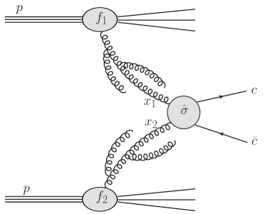
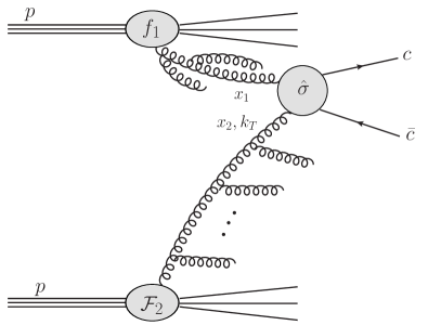
Figure 1: Left: gluon-gluon fusion process for charm production in hadron-hadron collisions in the collinear factorization approach. $f_{1},f_{2}$ are the integrated gluon distribution functions which depend on the longitudinal momentum fractions $x_{1},x_{2}$ and the hard scale of the partonic sub-process. Right: the same process, illustrated for the case of forward production in the $k_{T}$-factorization. The gluon $x_{1}$ is treated on-shell, and the gluon $x_{2}$ is off-shell with transverse momentum $k_{T}$. $\hat{\sigma}$ is the partonic cross section which is on-shell (left panel) and takes into account off-shellness of one gluon (right panel).

The production of charm in hadronic collisions is dominated by the gluon-gluon scattering. In this process, gluons from two colliding hadrons fuse and produce a charm quark-antiquark pair which subsequently fragments into the hadrons. The generic diagram for gluon-gluon fusion process in hadronic collision is illustrated in the left panel Fig. 1, where the cross section can be factorized into two gluon distribution functions, $f_{1}$ and $f_{2}$, and the perturbatively calculable partonic cross section $\hat{\sigma}$. This is the framework at the root of collinear factorization approach.

In the forward region, this process probes the kinematics where the two incoming partons have very different longitudinal momenta. The longitudinal momentum of the forward charm quark at high energy is approximately equal to $x_{F}\simeq E_{c}/E_{p}$ where $E_{p}$ is the energy of the incident proton and $E_{c}$ is the energy of the charm quark. Since we are interested in TeV-energy neutrinos from TeV-energy charm decay, the corresponding forward charm production kinematics probes values of $x_{F}$ of order $0.1$ or higher. This in turn means that the longitudinal momentum fraction of one of the gluons is large, $x_{1}\sim x_{F}$, and the other one is very small. To be precise the longitudinal momentum fraction $x_{2}\simeq m_{c\bar{c}}^{2}/(x_{F}s)$, where $m_{c\bar{c}}$ is the invariant mass of the produced charm-quark pair and $\sqrt{s}$ is the center of mass energy of the hadronic collision. This means that for high energies the forward production is particularly sensitive to the gluon density at very low values of $x_{2}\gtrsim 10^{-7}$, which is not constrained very well in this region. Thus the forward production offers unique possibilities for tests of novel QCD dynamics in the region of small-$x$.

III.1 Collinear Factorization at NLO

The double differential NLO cross-section for charm pair production is given by the expression

$$\frac{d^{2}\sigma_{pp}}{dydp^{2}_{T}}(s,m_{c}^{2})=\sum_{i,j=q,\overline{q},g}\int dx_{1}\,dx_{2}\,f_{i}(x_{1},\mu_{F}^{2})\,f_{j}(x_{2},\mu_{F}^{2})\,\frac{d^{2}\widehat{\sigma}_{ij}}{dydp^{2}_{T}}(\hat{s},m_{c}^{2},\mu_{F}^{2},\mu_{R}^{2})\,,$$ (2)

where $m_{c}$ is the charm mass, $\surd{\hat{s}}=\sqrt{x_{1}x_{2}s}$ is the partonic CM energy, $\mu_{F}$ and $\mu_{R}$ are the factorization and renormalization scales respectively, and $f_{i,j}$ represent the quark and gluon parton distribution functions (PDFs) as appropriate. As noted previously, we compute the cross-section to the next-to-leading order in perturbation theory.

The double differential cross-sections for charm quark production are calculated using the FONLL code Cacciari:1998it ; Cacciari:2001td , which provides an interface to LHAPDF Whalley:2005nh ; Buckley:2014ana , thus allowing one to use a variety of up-to-date PDFs. We choose to use the central CT14nlo PDF set Dulat:2015mca from the LHAPDF database as a representative set for our analysis. While there are more recent PDF sets available in the literature, including those that have been fit to 13 TeV LHCb data and consequently have reduced uncertainties in their predictions at low-$x$ Bertone:2018dse ; Zenaiev:2019ktw , we find that uncertainties in the cross-section from scale variation dwarf those from using different PDFs. Instead, our choice of the central CT14nlo PDF allows us to maintain compatibility with results obtained in Ref. Bhattacharya:2015jpa , while also using $m_{c}=1.3$ GeV, consistent with the PDG best-fit.

To obtain best-fits to current charm data, we choose to vary the factorization scale $\mu_{F}$ and renormalization scale $\mu_{R}$ while keeping the charm mass fixed. Assuming the scales vary proportionally to the charm transverse mass, $m_{T}={\left(m_{c}^{2}+p_{T}^{2}\right)}^{1/2}$, it has been the norm to vary these parameters independently within a range from $(0.5$–$2.0)\propto m_{T}$. However, when restricting ourselves to this narrow range, we find that at high energies $\sqrt{s}\geqslant 7$ TeV fits to data become progressively worse with increasing rapidities. Furthermore, determining uncertainties around the best-fit scales also requires one to extend the search beyond this range. Therefore, we allow these parameters to vary independently over a broader range $\in\left[0.5,8.0\right]$ unencumbered by theoretical preferences, allowing the best-fit parameters to be instead determined by fitting to data. We also determine the parameters defining a $1\sigma$ uncertainty band around the best-fit cross-section.

We compute cross-sections for a range of parameters $\left(\mu_{R},\mu_{F}\right)$ and obtain, for each choice of fragmentation scheme, the meson cross-section that may be fit to data from LHCb. The end result of this fitting exercise is that we obtain different sets of best-fit $\left(\mu_{R},\mu_{F}\right)$ for different fragmentation scheme. We defer the details of our fitting procedure to Appendix A.

III.2 $k_{T}$-factorization

In the forward regime, one should apply a framework which incorporates resummation of the large logarithms $\alpha_{s}\ln 1/x$. This is accomplished through the $k_{T}$-factorization formalism Catani:1990eg ; Catani:1990xk ; Collins:1991ty . The $k_{T}$-factorization formalism involves off-shell matrix-elements for partonic scattering and unintegrated gluon distribution functions ${\cal F}(x,{\bf k}_{T})$ which depend on the transverse momentum vector ${\bf k}_{T}$ of the off-shell gluons. The unintegrated gluon distribution functions encode more detailed information about the dynamics of the partons, and can be especially important in providing information about the details of the kinematics of the event. The $k_{T}$-factorization approach in hadroproduction of heavy quarks has been considered in Refs. Catani:1990eg ; Catani:1990xk ; Collins:1991ty where the off-shell matrix element for heavy quark production have been derived. The expression for the cross section in the $k_{T}$-factorization formalism has the following form, see e.g. Catani:1990eg

$$\sigma_{pp}(s,m_{c}^{2})=\int dx_{1}\,dx_{2}\,\frac{d^{2}{\bf k}_{1T}}{\pi}\,\frac{d^{2}{\bf k}_{2T}}{\pi}{\cal F}(x_{1},{\bf k}_{1T})\,{\cal F}(x_{2},{\bf k}_{2T})\,\widehat{\sigma}^{\rm off}(\hat{s},{\bf k}_{1T},{\bf k}_{2T},m_{c})\,$$ (3)

where the off-shell partonic cross section $\widehat{\sigma}^{\rm off}$ contains contributions from gluon-gluon scattering, dominant for the high energy limit. For the specific case of forward charm production considered here, due to the fact the kinematics is very asymmetric and one gluon has large longitudinal momentum fraction $x_{1}$ it is appropriate to use an approach in which this gluon is treated on-shell and satisfies the DGLAP evolution. Therefore the formula Eq. 3 in this limit becomes

$$\sigma_{pp}(s,m_{c}^{2})=\int dx_{1}\,dx_{2}\,\frac{d^{2}{\bf k}_{T}}{\pi}\,f(x_{1},\mu^{2})\,{\cal F}(x_{2},{\bf k}_{T})\,\widehat{\sigma}^{\rm on-off}(\hat{s},{\bf k}_{T},m_{c})\,,$$ (4)

where $\widehat{\sigma}^{\rm on-off}$ can be obtained from $\widehat{\sigma}^{\rm off}$ by setting one gluon on-shell, see Ref. Catani:1990eg . This is illustrated in the right panel of Fig. 1. The gluon with large longitudinal momentum fraction $x_{1}$ is indicated together with schematically drawn collinear cascade originating from one proton. On the other hand, the gluon with very small $x_{2}$ has transverse momentum $k_{T}$ and it is produced as a result of a very long cascade of emissions from the other proton. These emissions are not collinear, hence their transverse momenta are not ordered. Therefore such cascade leads to the diffusion in the transverse momentum distribution. This approach was used in Ref. Martin:2003us with the large $x_{1}$ gluon in the DGLAP collinear regime, which is on-shell and the small $x_{2}$ gluon off-shell, with appropriate approximation of the matrix element.

In this work we are interested in the differential distributions in rapidity, which can be obtained by generalizing collinear formula Eq. 2 to include the transverse momentum dependence. Since we are using expressions from Catani:1990eg , which are formally lowest order, the differential cross section can be taken as

$$\frac{d\sigma}{dy_{3}dy_{4}d^{2}{\bf p}_{3T}d^{2}{\bf p}_{4T}}=\int\frac{d^{2}{\bf k}_{T}}{\pi}\frac{\delta^{(2)}({\bf k}_{T}-{\bf p}_{3T}-{\bf p}_{4T})}{16\pi^{2}{(x_{1}x_{2}s)}^{2}}x_{1}g(x_{1},\mu^{2}){\cal F}(x_{2},{\bf k}_{T})\overline{\sum}|{\cal M}^{\rm on-offshell}_{gg^{*}\rightarrow c\bar{c}}|^{2}\;,$$ (5)

with momentum fractions $x_{1}=\frac{m_{3T}}{\sqrt{s}}\exp(y_{3})+\frac{m_{4T}}{\sqrt{s}}\exp(y_{4})$ and $x_{2}=\frac{m_{3T}}{\sqrt{s}}\exp(-y_{3})+\frac{m_{4T}}{\sqrt{s}}\exp(-y_{4})$ as well as the transverse masses $m_{3,4T}^{2}=p_{3,4T}^{2}+m_{c}^{2}$ of the quark and antiquark (see also Maciula:2022lzk ).

The unintegrated gluon distribution functions within the high-energy formalism need to be computed from the appropriate evolution equations which incorporate the small-$x$ dynamics. The unintegrated parton densities within the high energy formalism are usually computed from the Balitsky-Fadin-Kuraev-Lipatov (BFKL) equation which resums the powers of $\alpha_{s}\ln 1/x$ Kuraev:1977fs ; Balitsky:1978ic . It has been computed at leading logarithmic (LL) and next-to-leading logarithmic order (NLL) in QCD. For the phenomenological applications it needs to be supplemented by the additional corrections which take into account higher orders in the form of kinematical constraints and the constraints from matching to the DGLAP evolution Ciafaloni:2003rd . In addition, in the limit of high energies, or very small-$x$, other corrections are expected to occur, which are related to the parton saturation phenomenon Gribov:1983ivg . In this regime, the gluon densities are so large that recombination effects need to be taken into account which are expected to slow down the growth of the gluon densities. These corrections lead to the appearance of the non-linear terms in the small-$x$ evolution equations. The non-linear evolution leads to the taming of the gluon distribution in the region of very small-$x$ and moderate to small values of scales $k_{T}$. To be specific, these evolution equations generate the $x$-dependent saturation scale $Q_{s}^{2}(x)$. Whenever the relevant scale of the process, say the $k_{T}$ of the gluon, is smaller than $Q_{s}^{2}(x)$ non-linear terms are very important, while for $k_{T}^{2}>Q_{s}^{2}(x)$ they can be neglected and the non-linear evolution equations give results which coincide with thus obtained form the linear evolution.

The effective theory for high density at small-$x$ is the Color Glass Condensate McLerran:1993ka ; McLerran:1993ni ; Jalilian-Marian:1997jhx ; Jalilian-Marian:1997qno ; Iancu:2000hn ; Ferreiro:2001qy , with the corresponding JIMWLK evolution equations. In the multicolor limit the hierarchy of JIMWLK equations reduces to the Balitsky-Kovchegov equation Balitsky:1995ub ; Kovchegov:1999yj , the latter being the BFKL equation supplemented with the nonlinear term in the gluon density.

The small-$x$ unintegrated gluon density for the present paper was taken from Ref. Kutak:2012rf as well as from Ref. Li:2022avs . The gluon in Ref. Kutak:2012rf which was based on the unified BFKL+DGLAP evolution supplemented with small-$x$ resummation Kwiecinski:1997ee . Two sets of gluon distributions were used: based on linear evolution as well as non-linear evolution cast in the momentum space Kutak:2003bd ; Kutak:2004ym . The latter one includes the non-linear term in density which is responsible for the saturation effects. Both sets of distributions were fitted to the data on $F_{2}$ structure function at HERA. The non-linear term is important for low-$x$ and low values of transverse momenta and leads to taming of the gluon distribution and therefore the resulting observable cross section. We also used the gluon extracted from more recent fit in Ref. Li:2022avs to HERA data, which was based on the full resummation Ciafaloni:2003rd ; Ciafaloni:2003ek including the BFKL at NLO.

IV Charm Fragmentation

In the previous section we have discussed the perturbative aspects of charm production. We now turn to question of fragmentation of charm quarks into charm hadrons, which is a non-perturbative process and requires a separate treatment. Here we first review the standard fragmentation function formalism as well as its short-comings. We then present an alternative approach based on the modeling of hadronization in Monte Carlo generators.

IV.1 Fragmentation Functions

Many studies of charm production at the LHC make use of the factorization theorem to separate the charm production and fragmentation process. In the literature, the latter is then modeled via fragmentation functions that have been extracted from lepton collider data, assuming that they are also applicable at hadron colliders. As we will explain later, this may not be appropriate at hadron colliders, especially in forward and low transverse momentum region that is most relevant for FASER. In this approach, one uses the fact that charm quarks in electron-positron annihilation are produced with a known momentum, for example with $p_{c}=m_{Z}/2$ at LEP. One can then measure the flavor and momentum of charmed hadrons $p_{H}$ to constrain the fragmentation process. This is typically parameterized in terms of fragmentation fractions $f_{H}$, describing the probability of a charm quark to form a specific charm hadron $H$, and a fragmentation function $D_{H}(z)$, describing the distribution of fractional energy inherited by the hadrons $z=p_{H}/p_{c}$. In a later comparison of fragmentation approaches, we use the fragmentation fractions $f_{D^{+}}=0.244$, $f_{D^{0}}=0.606$, $f_{D_{s}^{+}}=0.081$ and $f_{\Lambda_{c}^{+}}=0.061$ as obtained in Ref. Lisovyi:2015uqa and the Peterson fragmentation function Peterson:1982ak . It has the form $D_{H}(z)\sim z^{-1}{[1-1/z-\epsilon/(1-z)]}^{-2}$ where we choose $\epsilon=0.035$ following Ref. ParticleDataGroup:2020ssz . Note that the same fragmentation function is used for all charmed hadrons. Simply for illustration, we will also consider the unphysical case with no fragmentation beyond fragmentation fractions. This means that quark and hadron momenta are identical, implying $D_{H}(z)=\delta(z-1)$.

Although the above-mentioned fragmentation functions approach has been successfully applied to measurements of charm production in the central and high-$p_{T}$ region of the LHC, it faces additional challenges in the forward and low-$p_{T}$ regime. There are a variety of hadron collision measurements that contradict the predictions obtained using fragmentation function; see Sec. 6.2.2 of Ref. Feng:2022inv for a pedagogical overview. In the following, we summarize three important observations that are particularly relevant for the modeling of forward charm production:

• The first observation concerns the production asymmetry of charmed mesons and their anti-particles. While the fragmentation function approach predicts equal production rates of charmed hadrons and their anti-particles, an excess of $D^{-}$ compared to $D^{+}$ has been observed at high $x_{F}$ in $\pi^{-}$-nucleus fixed target collisions recorded by WA82 WA82:1993ghz , E769 E769:1993hmj and E791 E791:1996htn . Such production asymmetries in the forward direction are typically explained by charm hadronization involving the beam remnants Norrbin:1998bw . In the case of $\pi^{-}$-nucleus collisions, the $\bar{c}$ can hadronize with the valence $d$ from the pion and form an energetic $D^{-}$ meson. In contrast the formation of a $D^{+}$ requires a $c$ and $\bar{d}$. Since the $\bar{d}$ cannot be a valence quark, but either a sea-quark or produced otherwise, the $D^{+}$ mesons are expected to be less energetic. This effectively induces a production asymmetry at high $x_{F}$.

• The second observation regards the energy spectra. Using the same data from pion fixed target experiments, it has been found that the momentum spectrum charm of hadrons are about as hard as or even harder than the charm quark spectra obtain from perturbation theory WA82:1993ghz ; E769:1993hmj ; E791:1996htn . This contradicts the fragmentation functions approach, which predict the hadrons to be softer than the charm quarks. In contrast, the above-mentioned mechanism of hadronization with other light quarks in the event, especially valence quarks from the beam remnant, would naturally allow the hadrons to be more energetic than the charm quarks and explain this observation.

• The third observation relates to the baryon to meson production ratios. Recently, ALICE has measured the ratio between the $\Lambda_{c}$ baryon and $D^{0}$ meson production rates in the central region and found that this ratio increases from about 10% at high transverse momentum to about 50% at low transverse momentum ALICE:2017thy ; ALICE:2020wla ; ALICE:2021rzj . A similar enhancement was also seen by CMS CMS:2019uws . This disagrees with the expectation from fragmentation functions applied in the lab frame and extracted from LEP, which predict a roughly constant $\Lambda_{c}$ to $D^{0}$ ratio of around 10%.

The observations above illustrate that fragmentation functions extracted from lepton colliders are not sufficient to describe charm production at hadron colliders.

IV.2 Hadronization using MC Generators

One way to address the abovementioned problems is to use more sophisticated models of fragmentation which are typically implemented in Monte Carlo generators. Here, we will take advantage of these efforts and use Pythia 8 Sjostrand:2006za ; Sjostrand:2014zea to model hadronization. Pythia uses the Lund string model Andersson:1983ia ; Sjostrand:1984ic in which colored objects are connected by a color string containing the field lines of the strong force. This model can intuitively explain two of the above observations: a charm quark connected to a beam remnant valence quark will be pulled forward, and hence gain energy, or even hadronize together with the valence quark, leading to a production asymmetry. By default, Pythia uses the Monash tune Skands:2014pea . While broadly used to describe phenomena at the LHC, we note that it is not able to properly describe the baryon enhancement observed at ALICE. This problem is addressed by a newer QCD-inspired color reconnection scheme introduced in Ref. Christiansen:2015yqa . It allows for different string topologies, such as junctions of three strings, which leads to a higher baryon production rates in high-multiplicity regions. It has been also recently suggested Kotko:2023ugv , using modeling with Pythia, that this QCD-inspired color reconnection mechanism might be essential for the proper description of the $J/\psi$ production at the LHC. Throughout this work, we use the mode 2 configuration introduced in Ref. Christiansen:2015yqa .

One practical complication is that the tools we use to model the perturbative production of charm quarks do not generate events that can be used as input to Pythia, but only provide the charm quark distribution $d^{2}\sigma_{c}/(dp_{T,c}dy_{c})$. We bypass this problem by using a re-weighting approach which is inspired by Refs. Gainer:2014bta ; Mattelaer:2016gcx . To understand the underlying idea, let us recall that, conceptually, we can write the charm hadron distribution $d^{2}\sigma_{H}/(dp_{T,H}dy_{H})$ as a convolution of the charm quark distribution $d^{2}\sigma_{c}/(dp_{T,c}dy_{c})$ and a (unitary) transfer function $f(\vec{p}_{c},\vec{p}_{H})$ describing the hadronization process:

$$\frac{d^{2}\sigma_{H}}{dp_{T,H}dy_{H}}=\int\frac{d^{2}\sigma_{c}}{dp_{T,c}dy_{c}}\times f(\vec{p}_{c},\vec{p}_{H})d\vec{p}_{c}.$$ (6)

In general, the transfer function would depend on both the quark and hadron momenta as well as the collider setup. In the fragmentation function approach, we assumed that $f=f_{H}\otimes D_{H}(z)$ and that it is independent of the collider setup. In Monte Carlo generators, the hadronization procedure is more complex and $f$ cannot be parameterized by a simple function. However, the transfer function is encoded in a generated event output: the charm production process of Pythia provides a sample of events, where each event is characterized by the parton momentum $\vec{p}_{c}$, the hadron momentum $\vec{p}_{H}$, a hadron ID and an event weight $w$. The events in the sample implicitly follow a distribution $d^{2}\sigma_{c}^{P8}/(dp_{T,c}dy_{c})$ for the charm quarks and $d^{2}\sigma_{H}^{P8}/(dp_{T,H}dy_{H})$ for the charm hadrons related via a Eq. 6 through a transfer function $f$.

To apply the same hadronization to a different model of charm production, we use the re-weighting procedure and adjust the weights

$$w\to w\times\frac{d^{2}\sigma_{c}/(dp_{T,c}dy_{c})}{d^{2}\sigma_{c}^{P8}/(dp_{T,c}dy_{c})}.$$ (7)

By construction, the events will then follow a $d^{2}\sigma_{c}/(dp_{T,c}dy_{c})$ at quark level. The hadrons follow the desired distribution

$$\int\frac{d^{2}\sigma^{P8}_{c}}{dp_{T,c}dy_{c}}\times\frac{d^{2}\sigma_{c}/(dp_{T,c}dy_{c})}{d^{2}\sigma_{c}^{P8}/(dp_{T,c}dy_{c})}\times f(\vec{p}_{c},\vec{p}_{H})\ d\vec{p}_{c}=\int\frac{d^{2}\sigma_{c}}{dp_{T,c}dy_{c}}\times f(\vec{p}_{c},\vec{p}_{H})\ d\vec{p}_{c}=\frac{d^{2}\sigma_{H}}{dp_{T,H}dy_{H}}\ ,$$ (8)

which we can extract from the event sample.

Let us summarize our approach. The usual fragmentation function approach assumes that the charm hadronization process is described by a transfer function of the specific form $f=D_{H}(z)$, which is universal for all colliders, applicable to all predictions of charm quark production, and independent of the charm quark kinematics and hadronic environment. We saw, however, that this assumption is invalid at hadron colliders. For example, hadronization with beam remnants, that is not captured in the fragmentation functions, leads to a harder forward charm hadron energy spectra and a charge asymmetry. This has been observed at past beam dump experiments and is expected to be important for forward charm hadron production at the LHC.

We therefore propose an alternative approach to model charm hadronization using Pythia, which only assumes that the underlying transfer function $f$ is the same for different predictions of charm quark production, and that Pythia provides a reasonably good prediction of hadronization especially in the forward direction. We note that the accuracy of Pythia’s description of forward charm hadronization, especially with beam remnants, has not yet been experimentally tested the hadronization process due to a lack of experimental data. However, Pythia’s good description of charm hadrons at beam dumps as well as light hadrons in the forward direction of the LHC LHCf:2017fnw ; LHCf:2017fnw provides some confidence in its overall description of hadronization.

V Results

In this section, we present and discuss the results of our different charm production models. We start this by systematically varying the modeling. For each considered setup, we shall show comparisons of our predictions to the double differential cross section of $D^{0}$ meson measured at 13 TeV by LHCb as well as the expected neutrino event rates at FASER$\nu$. To determine the neutrino flux, we follow the same approach as Ref. Kling:2021gos . Initially, the charm hadrons are decayed in their rest frame according to the decay branching fractions and energy distributions obtained with Pythia. Subsequently, the resulting neutrinos are boosted into the laboratory frame and recorded if they pass through the detector’s cross-sectional area. To obtain the anticipated number of neutrino interactions in the target volume, we convolute the neutrino flux with the interaction cross-sections obtained by GENIE Andreopoulos:2009rq . Here, we consider FASER$\nu$ to consist of a $25~{}\text{cm}\times 25~{}\text{cm}\times 1~{}\text{m}$ tungsten target FASER:2019dxq .

In the following, we will present results for collinear factorization in Sec. V.1 and $k_{T}$-factorization in Sec. V.2. We will compare both approaches and show additional distributions in Sec. V.3.

V.1 Collinear Factorization at NLO

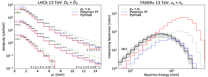
Figure 2: Modeling of Fragmentation: Predictions obtained using collinear factorization at NLO using the CT14nlo parton distribution functions. We show three different modeling approaches for fragmentation using only fragmentation fractions (green dotted), using the Peterson fragmentation function (blue dashed), and using Pythia with the QCD-inspired color reconnection scheme (red solid). For each approach, the scales were obtained using a fit to LHCb open charm data resulting in $(\mu_{F},\mu_{R})=(2.1,1.6)~{}m_{T}$ (no fragmentation function), $(\mu_{F},\mu_{R})=(3.75,1.75)~{}m_{T}$ (Peterson fragmentation function) and $(\mu_{F},\mu_{R})=(2.25,1.5)~{}m_{T}$ (Pythia). In the left panel, we compare these predictions with measurements of the double differential neutral D-meson production rate obtained by LHCb at 13 TeV. We present results for three different rapidity regions, where the results at higher rapidity were scaled. In the right panel, we show the resulting number of electron neutrinos from charm hadrons decay that interact with the FASER$\nu$ detector as a function of the neutrino energy. For context, we also display in black the event rate resulting from neutrinos from light hadron decays as obtained in Ref. Kling:2021gos . See the main text for a detailed discussion.

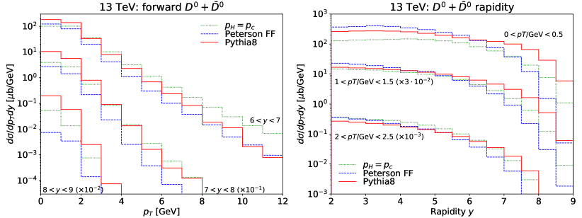
Figure 3: Predictions at High Rapidity: Predictions obtained using the same QCD parameters and the same fragmentation functions as in Fig.2, but for rapidity $y>6$ (left panel) and the rapidity distributions for small $p_{T}$ (right panel).

We first consider the calculation using the NLO collinear factorization. As described in Sec. III.1, we obtain multiple best-fit cross-sections corresponding to different fragmentation schemes. We find that a variation of the scale parameters $(\mu_{F},\mu_{R})$ mainly influences the normalization of the cross-section predictions, while the shape of the $p_{T}$ distribution remains largely unchanged. In contrast, the latter is more significantly affected by the choice of the fragmentation scheme.

We show a comparison of these results to the LHCb data in the left panel of Fig. 2 for three different modeling approaches for fragmentation. The green dotted line shows the best fit prediction obtained using a constant fragmentation factor. The best-fit cross-section in this case is obtained for $(\mu_{F},\mu_{R})=(2.1,1.6)\,m_{T}$ consistent with results from Bhattacharya:2015jpa . However, we find that the $p_{T}$ shapes of the corresponding double differential cross-sections are inconsistent with LHCb data, consistently overestimating at high $p_{T}$. With change of scales primarily affecting cross-section normalizations, and not the shape, there is no way to improve the fit within the realm of our analysis when using constant factors for fragmentation. Thus, this demonstrates the importance of including more realistic fragmentation schemes. The blue dashed lines show the best fit results using the Peterson fragmentation function, obtained for $(\mu_{F},\mu_{R})=(3.75,1.75)\,m_{T}$. These agree reasonably well with LHCb data for all rapidity regions, while still overestimating the data at low $p_{T}$ somewhat. Finally, best-fit results obtained using Pythia for fragmentation are shown as red solid lines. These correspond to $(\mu_{F},\mu_{R})=(2.25,1.5)\,m_{T}$. We observe that this setup produces similar results to those using the Peterson fragmentation function in the regime accessible to LHCb, with slight differences mainly at low $p_{T}<2~{}\text{GeV}$.

We proceed to evaluate the electron neutrino flux from charm hadron decay at FASER$\nu$ from these simulations. The results are shown in the right panel of Fig. 2. With Peterson’s fragmentation, the obtained flux has lower rates and peaks at lower energies compared to the scenario without any fragmentation. This outcome is expected since in the fragmentation function approach, the charm hadron is always less energetic than the charm quark. In contrast, using Pythia for fragmentation increases the neutrino flux and shifts it to higher energies compared to the scenario without any fragmentation. As discussed in Sec. IV, this outcome is consistent with observations at beam dump experiments, where hadronization with beam remnants plays a role. We emphasize that despite both fragmentation choices providing similarly good descriptions of the LHCb data, they lead to a significant difference in neutrino event rates at FASER$\nu$, differing by about one order of magnitude. This highlights the importance of properly modeling fragmentation for forward charm and, consequently, neutrino flux predictions for FASER$\nu$ and other LHC neutrino experiments. For comparison, we also show the event rate from light hadron decays in black, as obtained in Ref. Kling:2021gos , using various generators. The solid line represents the central prediction, while the shaded band shows the range of predictions from different generators. This line is meant to provide optical guidance and to illustrate regions where light and charm hadron decay contributions dominate the electron neutrino flux.

While our prediction already agrees reasonably with the LHCb data, we observe an underestimation of events at intermediate $p_{T}\sim 8~{}\text{GeV}$ and a mild overestimation at $p_{T}\sim 1~{}\text{GeV}$ when compared to experimental measurements. As pointed out in Ref. Bai:2020ukz , including an additional $k_{T}$ smearing, which aims to capture both an intrinsic transverse momentum of the initial state partons as well as some soft gluon emission effects, can help improve the agreement with data. The authors achieve this by introducing a Gaussian smearing with width $\langle k_{T}\rangle$ of the transverse momentum of the charm, while keeping its rapidity constant. However, we note that this approach does not conserve energy and can lead to charm quarks that are more energetic than the proton beam. Indeed, this leads to an unphysical order of magnitude increase of the neutrino event rate at high energies. To address this issue, we modify the smearing such that the $z$ component of charm quark momentum is kept constant and the rapidity is allowed to change.

By iterating over a range of values of $\langle k_{T}\rangle$ (see Appendix B), we find that the best agreement to data is for a combination of $\langle k_{T}\rangle=1.5~{}\text{GeV}$ and $(\mu_{F},\mu_{R})=(1.75,1.25)~{}m_{T}$. This value of $\langle k_{T}\rangle$ is consistent with Ref. Bai:2022xad , which uses $\langle k_{T}\rangle=1.2~{}\text{GeV}$, as well as with the default transverse momentum for hard interactions used within Pythia, which is $1.8~{}\text{GeV}$. The corresponding neutrino fluxes are not highly sensitive to the choice of $\langle k_{T}\rangle$.

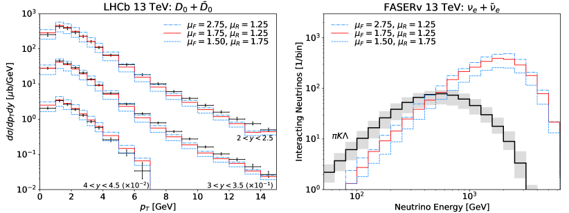
Figure 4: Scale Variation in Collinear Factorization: Predictions using collinear factorization at NLO with different choices of scales $\mu_{F}$ and $\mu_{R}$. All prediction use the CT14nlo parton distribution function, $k_{T}$ smearing with $\langle k_{T}\rangle=1.5~{}\text{GeV}$ and Pythia with the QCD-inspired color reconnection scheme to model fragmentation. See the main text for a detailed discussion.

In order to illustrate why different fragmentation approaches give similar results for the LHCb data, but very different neutrino flux in the forward region, we show $p_{T}$ distribution for large $y>6$ and the rapidity distributions for low $p_{T}$ in Fig. 3. We note that for lowest value of $p_{T}$ and large rapidity, calculations with various fragmentation schemes differ significantly.

Up to now, we’ve only shown our central prediction, which uses scale choices $(\mu_{F},\mu_{R})=(1.75,1.25)~{}m_{T}$ that were obtained by fitting the data with $\langle k_{T}\rangle=1.5~{}\text{GeV}$. The same fit also allows to define scale uncertainties in a data driven way (see Appendix A for details). To illustrate this, we present in Fig. 4 our results for two additional scale choices, which provide an error band that encompasses the LHCb data. Looking at the right panel, the corresponding neutrino fluxes show only mild sensitivity to the choice of scales.

V.2 $k_{T}$-Factorization

We have observed that introducing an additional $k_{T}$ smearing improves the agreement of the collinear factorization prediction with data. This smearing effectively simulates intrinsic transverse momentum and soft-gluon emissions in the initial state. These effects are naturally included in the $k_{T}$-factorization approach due to the presence of the unintegrated gluon distribution function and the off-shell matrix element which depend on transverse momentum $k_{T}$. As discussed in Sec. III.2, we are using a hybrid approach which utilizes an unintegrated PDF for the low-$x$ gluon and an integrated PDF for the high-$x$ gluon. This is because ultimately we are interested in the very forward region where one $x$ is very small and the other very large.

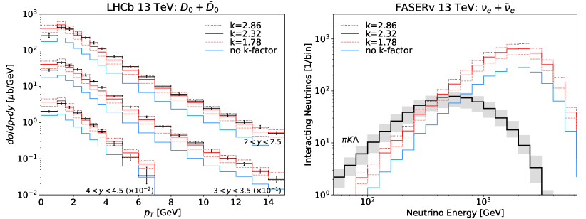
Figure 5: Normalization in $k_{T}$-Factorization: Predictions using $k_{T}$-factorization before (blue) and after (red) applying an overall $k$-factor. These predictions use we use the KS (non-linear) unintegrated distribution for the low-$x$ gluon, CT14nlo for the high-$x$ gluon and use Pythia with the QCD-inspired color reconnection scheme to model fragmentation. See the main text for a detailed discussion.

As the basic setup we choose the unintegrated gluon distribution from the Kutak-Sapeta (KS) calculation Kutak:2012rf using the nonlinear evolution, and for the large-$x$ we use the CT14nlo gluon. Since the KS gluon has been fitted to the HERA data using the leading order strong coupling constant, we use the same setup for the one power of strong coupling in the formula for the cross section. The second power of the coupling is taken at NLO consistent with the CT14nlo PDF used for large-$x$ gluon. As before we are are modeling the hadronization using Pythia with the QCD-inspired color reconnection scheme. The results are shown in Fig. 5 by the blue curve. We observe that the calculation has the right shape in $p_{T}$ but it significantly underestimates the experimental data. This was also observed in calculation of Maciula:2022lzk . This is not totally unexpected since the off-shell partonic cross section used in $k_{T}$-factorization is effectively computed at the LO Catani:1990eg . Therefore when compared with NLO collinear calculation it does not have virtual terms as well as final state gluon emissions from the quarks. It also has an off-shell gluon only on the small-$x$ side. Given that the NLO calculation in the collinear approach resulted in $K$-factor of the order of $2.5$ with respect to the LO result, see e.g. Nason:1987xz , it is expected that the $k_{T}$-factorization will likely have large $K$-factor as well.

In order to get the normalization to agree with LHCb data, and therefore make our extrapolations from LHCb to FASER$\nu$ more reliable, we introduce a normalization factor which we refer to as $k$-factor in this calculation, determined by a fit to the data (with additional weights that ensure each rapidity bin contributes identically to the $\chi^{2}$ measure). We find a best fit of $k=2.32$; the resulting double-differential cross-section is illustrated by red line in Fig. 5. This is in excellent agreement with the LHCb data over the full $p_{T}$ and rapidity range. This is encouraging since it means that the $x$ dependence of the unintegrated gluon, correctly reproduces the rapidity dependence, and also the $p_{T}$ dependence is correctly captured. We shall also see, that the $k$-factor does not change between the $7$ and $13$ TeV. We also determine an uncertainty of the fit, as illustrated by the orange and magenta curves in the same figure (using a rescaled $\chi^{2}$ for this following the PDG procedure described in Refs. ParticleDataGroup:2020ssz ; Rosenfeld:1975fy ). These variations form a nice envelope around the data with a width of about a factor 2 at low values of $p_{T}$. The right panel in Fig. 5 shows the electron neutrino flux obtained in this approach. A similar size band is also obtained at FASER$\nu$, see right panel.

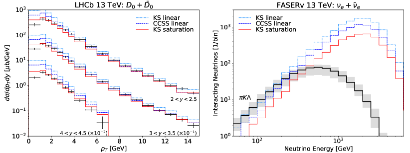
Figure 6: Low-$x$ Gluon Distribution in $k_{T}$-Factorization: Predictions using $k_{T}$-factorization using the KS (blue dot-dashed) and CCSS (blue dashed) unintegrated distribution with a purely linear evolution as well as the KS unintegrated distribution including non-linear effects that describe saturation effects (red solid) for the low-$x$ gluon. All predictions use a constant $k$-factor of $2.32$, the CT14nlo parton distribution function for the high-$x$ gluon, use Pythia with the QCD-inspired color reconnection scheme to model fragmentation. See the main text for a detailed discussion.

Next, we study the dependence of the results on the choice of the low-$x$ unintegrated gluon distribution. In Fig. 6 we show our results for three choices of unintegrated PDFs: two choices for the KS gluon with linear evolution and with non-linear effects that describe saturation effects, and third choice of gluon from Li:2022avs obtained from the linear evolution including the resummation using the Ciafaloni-Colferai-Salam-Stasto (CCSS) approach Ciafaloni:2003rd . We find that the prediction which includes saturation effects is in excellent agreement with the LHCb data over the full $p_{T}$ range. In contrast, the linear cases overshoot the data at low $p_{T}$. However, given that the results include the $k$-factor effectively added by fitting as explained before, it is not possible to conclude at this moment about the importance of the saturation effects in the LHCb data. Looking at the right panel, including saturation effects results in a reduction of the flux by a factor of approximately three compared to the linear case. This is due to the fact that the nonlinear effects are largest at very low $p_{T}$.

We have also tested the sensitivity of the $k_{T}$ factorization calculations to the choices of the large $x$ gluon distribution, the running coupling order and the scale choice. The results of these studies are collected in Appendix C. We have found rather small differences between the calculations for these various choices.

V.3 Comparison of Approaches

Based on the previous discussion, we identify central predictions for both factorization approaches. In particular, we consider the following configuration

• collinear factorization at NLO with CT14nlo for the gluon parton distribution, renormalization scale $\mu_{R}=1.75~{}\text{m}_{T}$, factorization scale $\mu_{F}=1.25~{}m_{T}$, a $k_{T}$ smearing with $\langle k_{T}\rangle=1.5~{}\text{GeV}$, and fragmentation modeled with Pythia with the QCD-inspired color reconnection scheme

• $k_{T}$-factorization using KS unintegrated distribution for the low-$x$ gluon including saturation effects, the CT14nlo parton distribution for the high-$x$ gluon, a $k$-factor of $2.32$ and fragmentation modeled with Pythia with the QCD-inspired color reconnection scheme

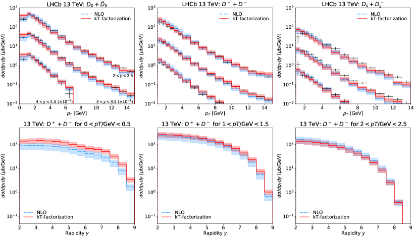
Figure 7: Comparison of Charm Hadron Distribution at 13 TeV: Predictions using collinear factorization at NLO and $k_{T}$-factorization. The shaded band around the NLO predictions corresponds to the scale variations shown in Fig. 4 while the shaded band around the $k_{T}$-factorization prediction corresponds to a varation of the $k$-factor as shown in Fig. 5. In the top row, we show the $p_{T}$ distributions for all three charmed mesons in comparison to LHCb data. The bottom row show the rapidity distribution for $D^{\pm}$ mesons in three transverse momentum regions.

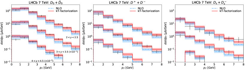
Figure 8: Comparison of Charm Hadron Distribution at 7 TeV: Transverse momentum distributions for all three charmed mesons in comparison to 7 TeV LHCb data using the same collinear factorization at NLO and $k_{T}$-factorization setups as in Fig. 7.

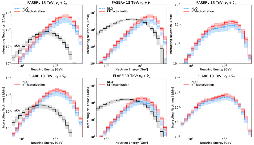
Figure 9: Comparison of Forward Neutrino Distributions: Forward neutrino flux predictions using the same collinear factorization at NLO and $k_{T}$-factorization setups as in Fig. 7. The energy spectra of neutrinos interacting in FASER$\nu$ at Run 3 of the LHC are shown in the top row for all three neutrino flavors. Similar distributions for proposed FLARE detector at FPF during the HL-LHC era are shown in the bottom row.

In Fig. 7, we compare the corresponding distributions from both approaches. We note that $k_{T}$-factorization with saturation gives slightly better description of the $p_{T}$ shape of the LHCb data than the NLO case. However, we again remind the reader, that this has to be taken with caution since this calculation includes the fitted $k$-factor which is not needed for the NLO collinear approach. We find that both approaches give good description of $D^{0}+\bar{D^{0}}$ data but when compared with LHCb data for $D^{+}+D^{-}$, and for $D_{s}+D_{s}^{-}$, the low $p_{T}$ region is overestimated. We show distributions as a function of rapidity for different $p_{T}$ regions, and we find that NLO and $k_{T}$-factorization with saturation give similar values for central rapidity, but they differ at large rapidity, by about a factor of $2$, especially for $0<p_{T}<0.5$ region. For large values of $p_{T}$, this difference is reduced.

In Fig. 8, we also show comparison of both approaches with the LHCb data at 7 TeV, and the description is very good in both cases. It should be stressed that the used scales for the NLO calculation and the $k$-factor for $k_{T}$-factorization at $7$ TeV are the same as extracted from $13$ TeV data. As mentioned previously, this is encouraging since it means that the energy dependence of the data, which is driven mainly by the $x$ evolution of the unintegrated gluon density is captured correctly. The latter one has been taken from the resummed approaches Kwiecinski:1997ee ; Ciafaloni:2003ek ; Ciafaloni:2003rd which aim to reproduce both small-$x$ and collinear dynamics.

The neutrino flux obtained using both QCD approaches is presented in Fig. 9. The upper row shows the number of interacting neutrinos in FASER$\nu$ operating during LHC Run 3 with an integrated luminosity of $150~{}\text{fb}^{-1}$ while the bottom row shows the neutrino events rate at FLARE at the FPF during the HL-LHC with a luminosity of $3~{}\text{ab}^{-1}$. The three columns correspond to the three neutrino flavors. The shape of the neutrino flux remains similar for all neutrino flavors in both approaches, with the NLO contribution slightly lower than that of the $k_{T}$-factorization. However, the two approaches are very close and fall within the range of uncertainty, which is approximately a factor of two. The black lines represent the contribution to the neutrino flux from decays of light hadrons. Notably, we find that the dominant contribution to neutrinos occurs above $500~{}\text{GeV}$ for $\nu_{e}$ and above $1~{}\text{TeV}$ for $\nu_{\mu}$. Detecting $\nu_{\tau}$ would serve as a direct test of charm production, as there is no contribution from pions and kaons decays.

Based on our calculation, we predict that FASER$\nu$ during LHC Run 3 is expected to observe approximately $4000~{}\nu_{e}$, $4000~{}\nu_{\mu}$, and $120~{}\nu_{\tau}$ charge current interactions originating from decays of charm hadrons. The FPF, proposed to house larger neutrino detectors during the HL-LHC era, aims to record a significantly larger sample of neutrino interaction events Anchordoqui:2021ghd ; Feng:2022inv . Specifically, we consider the FLARE detector housed within the FPF, for which we assume a $1~{}\text{m}\times 1~{}\text{m}\times 7~{}\text{m}$ liquid argon target Feng:2022inv . We can see that FLARE will detect approximately $1.4\times 10^{5}~{}\nu_{e}$, $1.4\times 10^{5}~{}\nu_{\mu}$, and $6000~{}\nu_{\tau}$ from charm hadron decays. This substantial increase in statistics will enable FPF experiments to conduct more detailed tests on forward charm production and provide the necessary data to distinguish between different predictions.

VI Conclusion

Forward charm production at hadron colliders has long been recognized as an sensitive tool for probing the strong interaction. However, until recently, it has remained beyond the reach of the existing LHC experiments. This situation is now changing with the start of operation of the FASER$\nu$ and SND@LHC experiments, which are strategically positioned in the far-forward direction of the LHC and specifically designed to detect collider neutrinos. Many of these neutrinos originate from the decay of charm hadrons, presenting a unique opportunity to investigate forward charm production. Together, FASER$\nu$ and SND@LHC are projected to observe approximately ten thousand neutrinos during the LHC’s Run 3, spanning from 2022 to 2025. Looking forward, a continuation of this collider neutrino program is envisioned for the HL-LHC era from 2029 to 2042: by utilizing larger detectors situated in the FPF it will be possible to detect millions of collider neutrinos.

In this work, we have predicted neutrino fluxes from charmed mesons in these forward neutrino experiments. To this end, we have modeled charm hadron production from $pp$ collisions at 13 TeV using different QCD and hadronization models, fitting our hadron cross-sections to charmed meson data from LHCb to ascertain the values of parameters involved in our models. This also allows us to determine which QCD and hadronization models are well tailored to describing physics at the forward rapidities that will be probed at FASER$\nu$.

When evaluating hadron cross-sections against current collider data, we have placed particular emphasis on the hadronization models used to convert charm cross-sections to hadronic ones. We have discussed how current fragmentation function based models in the literature are not especially well motivated to describing far forward physics, because, among other things, they omit the potential for involving beam remnants when hadronizing. With the end goal of accurately forecasting neutrino fluxes at FASER$\nu$, we have, instead, devised a scheme that employs the string fragmentation model implemented in Pythia 8, resulting in a more realistic representation of hadronization. This Pythia-based scheme naturally overcomes most of the theoretical shortcomings of fragmentation function based models. We also demonstrate that the use of this hadronization scheme leads to a significantly enhanced flux of forward neutrinos compared to those obtained using established fragmentation functions, which results from allowing the hadronization with beam remnants. This underscores the importance of utilizing an accurate fragmentation modeling. However, we also note that the topic of forward charm hadronization warrants further theoretical investigation.

To obtain the charm cross-sections that underpin our analysis, we have investigated two distinct QCD models and made noteworthy improvements to each insofar as they apply to forward physics:  a) collinear factorization, where we use factorization and renormalization scales as free parameters to be determined by fitting to LHCb data, as is typically done in the literature, but in addition apply a $k_{T}$ smearing on the charm transverse momentum in an energy conserving way; and  b) $k_{T}$factorization, which is more suitable for the description of the forward particle production at high energy since it resums contributions due to the small $x$ effects in the parton density, and where we include a $k$-factor to account for a mismatch in the normalization against LHCb data. When using the former, we find that — no matter the variation of scales — the agreement of the shape of final hadron differential cross-sections vis-à-vis LHCb data is noticeably improved by the allowing a Gaussian smearing of the charm transverse momentum with some mean $k_{T}$. In contrast with Ref. Bai:2020ukz , where this $k_{T}$ smearing effect has been first discussed, our analysis explicitly conserves energy when applying the transformation by keeping the charm $z$-momentum constant and allowing its rapidity to vary. We find a best-fit to 13 TeV LHCb data is obtained for $\{\mu_{F},\mu_{R}\}=\{1.75,1.25\}m_{T}$ alongwith $\langle k_{T}\rangle=1.5~{}\text{GeV}$. When using the $k_{T}$ factorization scheme, our central prediction incorporates the KS unintegrated distribution with a non-linear evolution for the low-$x$ gluon, and the CT14nlo distribution for large-$x$ gluons. A salient feature of our analysis is that, in order to describe the LHCb data, we introduce a constant $k$-factor of $2.32$, determined by fitting the overall normalization to data. The need for the inclusion of the normalization $k$-factor in $k_{T}$-factorization approach likely stems from the fact that the off-shell partonic cross section for production of heavy quarks is only available at lowest order. To theoretically ascertain the value of the $k$-factor, higher orders of the off-shell partonic cross section will need to be computed, and possibly resummed. We further examined the impact of systematically varying the underlying QCD parameters, such as scale selection and parton distribution function choices at low and high $x$ on these predictions.

We note that both QCD approaches provide a good description of the LHCb data when paired with the PYTHIA hadronization scheme. They exhibit similar energy dependence in the neutrino flux with slightly different overall normalizations, which can be attributed to the specific QCD parameter choices. More theoretical work with respect to the underlying uncertainties relevant to each model is needed to improve the precision of these calculations (in particular the small $x$ approach), as well as further experimental input in order to distinguish between NLO collinear and $k_{T}$-factorization, and especially to see an onset of parton saturation.

Using our best-fit QCD models, we have shown predictions for neutrino fluxes of all three flavors for the ongoing FASER experiment as well as the proposed FLARE detector at the FPF and compared them against those from the decay of lighter mesons. We find that, depending on the choice of QCD scheme, the electron neutrino flux from charmed mesons dominates over those from pions and kaons starting at neutrino energies between 400 and 500 GeV. Furthermore, muon neutrinos from charmed meson decay become comparable to those from pion and kaon decays at energies above 1 TeV for both QCD approaches. Tau neutrinos, produced exclusively from heavy meson decays, provide a background-free channel to investigate heavy meson QCD. Our models predict between 4000 and 6000 charged current tau neutrino interactions at FLARE with energies around 1 TeV, depending on whether one uses the collinear NLO scheme or the $k_{T}$-factorization scheme respectively.

The first observation of collider neutrinos at FASER FASER:2023zcr heralds the opening of a new frontier towards significantly improved understanding of forward QCD. Further measurements at both FASER and SND@LHC will provide a unique opportunity to gather valuable information about small-$x$ QCD, validity of $k_{T}$-factorization and NLO collinear approach, and validity of different hadronic fragmentation scenarios at forward rapidities. In the future, the planned experiments at the FPF, with significantly improved statistics, will become the ideal place to unravel these most important facets of QCD. In addition, we expect that measurements of the forward neutrino production at the LHC will provide valuable inputs for estimating the prompt neutrino flux, reducing its theoretical uncertainties and thus providing a better understanding of the main background for the detection of ultra-high energy neutrinos be it from extragalactic astrophysical sources or from beyond standard model physics including dark matter decays and annihilation.

Appendix A Variation of parameters in the collinear factorization

To determine the correct global best-fits for these scales, one ought to use all the available data for charm production in $pp$ collisions and determine the cross-section that gives the least value of $\Delta\chi^{2}$. However, for our specific study where predictions for the forward neutrino flux are the end goal, we need cross-sections that accurately describe the data at high energies $\sqrt{s}\sim 13$ TeV and high rapidities. The highest rapidity $d^{2}\sigma/dydp_{T}$ data at 13 TeV come from charmed meson cross-sections observed at LHCb LHCb:2015swx . These include cross-sections for $D^{0},D^{\pm},\text{ and }D_{s}$ at rapidities between $2\leqslant y\leqslant 4.5$ binned by $0.5$, i.e. five bins in $y$ for each meson. We focus on this subset of collider data to determine the scales, $\mu_{R}$ and $\mu_{F}$, that best describes it.

To compare our theoretical cross-sections against charmed meson cross-sections from LHCb, we first compute the double differential cross-section $d^{2}\sigma_{c\bar{c}}/dydp_{T}$ for bare $c\bar{c}$ pair production using specific values for the fragmentation and renormalization scales. We then assume a specific fragmentation scheme, without any additional free parameters, to hadronize the charm quarks into hadrons. The resulting differential cross-section distribution at this stage may now be compared against corresponding LHCb data for a measure of its goodness of fit, which we achieve by means of a simple $\chi^{2}$ analysis. Since accurately forecasting high rapidity cross-sections is critical towards obtaining predictions for forward experiments like FASER, it becomes important to ensure that the goodness of fit analysis is not skewed by the availability of significantly more data at LHCb’s lower rapidities $2\leqslant y\leqslant 3$ rather at, say, $y\geqslant 4$. We therefore use a $\chi^{2}$ measure that is normalized to the number of $p_{T}$ bins with cross-section measurements for each rapidity bin in the LHCb data, ensuring that each bin carries equal weight towards the measure.

Repeating this procedure for multiple $\left(\mu_{R},\mu_{F}\right)$ values, we generate a range of cross-sections and, for a given fragmentation scheme, we ascertain the best-fit value of these parameters as the one that minimizes the $\chi^{2}$/d.o.f. Likewise, we also obtain the parameters corresponding to a $1\sigma$ region of variation around the best-fit cross-section. The gives us a set of best-fit $\left(\mu_{R},\mu_{F}\right)$ parameters for each choice of fragmentation scheme.

Appendix B $k_{T}$ smearing in collinear factorization

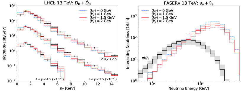
Figure 10: Smearing of ${\bf k}_{T}$ in Collinear Factorization: Predictions using collinear factorization at NLO including $k_{T}$ smearing for different values of $\langle k_{T}\rangle$. All predictions use fixed scales $(\mu_{F},\mu_{R})=(1.75,1.25)~{}m_{T}$, the CT14nlo parton distribution function and Pythia with the QCD-inspired color reconnection scheme to model fragmentation. See the main text for a detailed discussion.

In Fig. 10, we present our results when applying the smearing with different values of $\langle k_{T}\rangle$ to our central prediction. In this case, when using $\langle k_{T}\rangle=1.5~{}\text{GeV}$, our fitting routine leads to a best-fit $(\mu_{F},\mu_{R})=(1.75,1.25)~{}m_{T}$. As shown in the left panel, the shape of the transverse momentum distributions in the LHCb range changes: events are shifted from the lowest $p_{T}$ bins towards intermediate $p_{T}$ bins. This effect becomes stronger with increasing $\langle k_{T}\rangle$, and by scanning fits made using different fixed values for $\langle k_{T}\rangle=0,0.5,1.0,1.5,2.0\ldots$, we find that the best agreement with data is obtained for $\langle k_{T}\rangle=1.5~{}\text{GeV}$. As shown in the right panel of Fig. 10, the corresponding neutrino fluxes are not highly sensitive to the choice of $\langle k_{T}\rangle$.

Appendix C Variation of parameters in the $k_{T}$ factorization calculation

In this appendix we include the tests of the $k_{T}$ factorization approach while varying the large $x$ gluon distribution, the order of the running coupling and the choice of the scales.

In Fig. 11, we explore the impact of the choice of integrated gluon distributions used for the high-$x$ region, while keeping the unintegrated PDF with saturation for the low-$x$ gluon fixed. We consider four different choices consisting of the CT14 and NNPDF30 distributions at both leading and next-to-leading order. Our results show that the next-to-leading order distributions provide a somewhat better description of the LHCb data. In contrast, the leading order distributions tend to overestimate the production rate at low $p_{T}$, leading to an increased neutrino flux. We observe small variations within the same order of distributions, with a corresponding uncertainty of about $20-25~{}\%$ at the peak of the flux. Therefore we choose the NLO PDFs in the calculation as our standard choice and for a better accuracy.

Next, in Fig. 12 we study the dependence of the $k_{T}$-factorization calculation on the choice of the order at which the strong coupling is taken as well as the value of $\Lambda_{QCD}$. Our standard choice is denoted by the ‘hybrid’ in Fig. 12. As mentioned previously this choice amounts to taking one power of the strong coupling in the leading order. This is consistent with the choice used in the fit used to extract the unintegrated KS gluon density in Kutak:2012rf . The second power of the strong coupling is taken consistent with the choice of the large-$x$ gluon PDF, in this case CT14nlo set. We also compare this with two other choices, one in which both powers of $\alpha_{s}$ are taken at leading order and one in which they are taken at NLO from CT14nlo, labeled as LO and NLO in Fig. 12, respectively. We see that these different choices give a moderate spread in the predictions. We remind here that we are using the same $k$-factor for all of these predictions, in order to isolate the dependence on the coupling choice. The shape in $p_{T}$ is affected only modestly, mainly in the low $p_{T}$ region. In the right panel in Fig. 12 we again show the spread of about factor of order $2$ in the neutrino flux predictions.

Finally, we study the dependence on the variation of the scale in the large-$x$ PDF and in the argument of the strong coupling. We vary the scale in the region $(0.5,2.0)\langle p_{T}^{2}\rangle$ where we define $\langle p_{T}^{2}\rangle=(p_{T1}^{2}+p_{T2}^{2})/2$, and $p_{T1},p_{T2}$ are the transverse momenta of the produced quark and antiquark. The results are demonstrated in Fig. 13. We observe that the variation of scales has very little impact on both the $p_{T}$ dependent cross section at LHCb as well as on the neutrino results at FASER$\nu$.

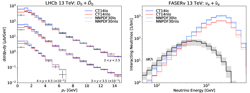
Figure 11: High-$x$ Gluon Distribution in $k_{T}$-Factorization: Predictions using $k_{T}$-factorization based on different parton distribution of the high-$x$ gluon. All predictions use a constant $k$-factor of $2.32$, the KS (non-linear) unintegrated distribution for the low-$x$ gluon and Pythia with the QCD-inspired color reconnection scheme to model fragmentation. See the main text for a detailed discussion.

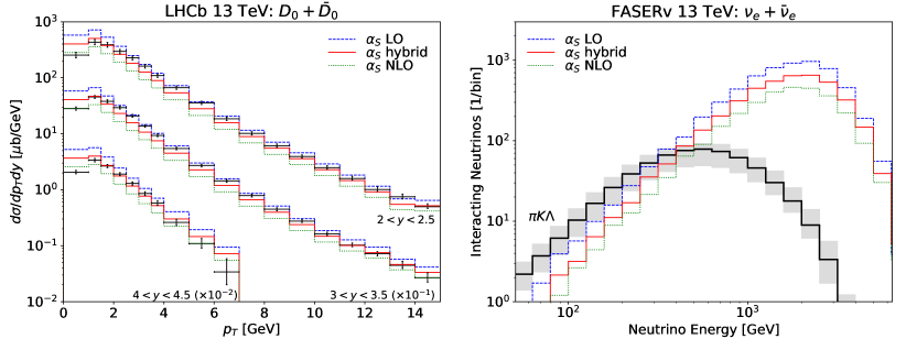
Figure 12: Strong Coupling in $k_{T}$-Factorization: Predictions using $k_{T}$-factorization using different choices of the strong coupling: ‘hybrid’ (one power of coupling at LO and one power at NLO ), ‘LO’ (both powers of strong coupling at LO) and ‘NLO’ (both powers of strong coupling at NLO corresponding to the large-$x$ PDF). All predictions use a constant $k$-factor of $2.32$, the KS (non-linear) unintegrated distribution for the low-$x$ gluon, CT14nlo for the high-$x$ gluon and Pythia with the QCD-inspired color reconnection scheme to model fragmentation. See the main text for a detailed discussion.

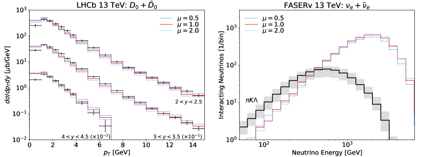
Figure 13: Scale Choice in $k_{T}$-Factorization: Predictions using $k_{T}$-factorization using scale choice of $\mu\,\times\,\langle p_{T}^{2}\rangle$, with $\langle p_{T}^{2}\rangle=(p_{T1}^{2}+p_{T2}^{2})/2$ and values of $\mu=0.5,1.0,2.0$ for dashed-blue, solid-red and dotted-blue curve respectively. All predictions use a constant $k$-factor of $2.32$, the KS (non-linear) unintegrated distribution for the low-$x$ gluon, CT14nlo for the high-$x$ gluon and Pythia with the QCD-inspired color reconnection scheme to model fragmentation. See the main text for a detailed discussion.

References

- (1) H1, ZEUS Collaboration, F. D. Aaron et al., “Combined Measurement and QCD Analysis of the Inclusive e+- p Scattering Cross Sections at HERA,” JHEP 01 (2010) 109, arXiv:0911.0884 [hep-ex].
- (2) A. D. Martin, M. G. Ryskin, and A. M. Stasto, “Prompt neutrinos from atmospheric and production and the gluon at very small x,” Acta Phys. Polon. B 34 (2003) 3273–3304, arXiv:hep-ph/0302140.
- (3) L. V. Gribov, E. M. Levin, and M. G. Ryskin, “Semihard Processes in QCD,” Phys. Rept. 100 (1983) 1–150.
- (4) A. Bhattacharya, R. Enberg, M. H. Reno, I. Sarcevic, and A. Stasto, “Perturbative charm production and the prompt atmospheric neutrino flux in light of RHIC and LHC,” JHEP 06 (2015) 110, arXiv:1502.01076 [hep-ph].
- (5) R. Gauld, J. Rojo, L. Rottoli, and J. Talbert, “Charm production in the forward region: constraints on the small-x gluon and backgrounds for neutrino astronomy,” JHEP 11 (2015) 009, arXiv:1506.08025 [hep-ph].
- (6) M. V. Garzelli, S. Moch, and G. Sigl, “Lepton fluxes from atmospheric charm revisited,” JHEP 10 (2015) 115, arXiv:1507.01570 [hep-ph].
- (7) IceCube Collaboration, R. Abbasi et al., “The IceCube high-energy starting event sample: Description and flux characterization with 7.5 years of data,” Phys. Rev. D 104 (2021) 022002, arXiv:2011.03545 [astro-ph.HE].
- (8) ATLAS Collaboration, G. Aad et al., “Measurement of , and meson production cross sections in collisions at TeV with the ATLAS detector,” Nucl. Phys. B 907 (2016) 717–763, arXiv:1512.02913 [hep-ex].
- (9) CMS Collaboration, A. M. Sirunyan et al., “Nuclear modification factor of D0 mesons in PbPb collisions at TeV,” Phys. Lett. B 782 (2018) 474–496, arXiv:1708.04962 [nucl-ex].
- (10) CMS Collaboration, A. Tumasyan et al., “Measurement of prompt open-charm production cross sections in proton-proton collisions at = 13 TeV,” JHEP 11 (2021) 225, arXiv:2107.01476 [hep-ex].
- (11) ALICE Collaboration, S. Acharya et al., “Measurement of D-meson production at mid-rapidity in pp collisions at TeV,” Eur. Phys. J. C 77 (2017) no. 8, 550, arXiv:1702.00766 [hep-ex].
- (12) ALICE Collaboration, S. Acharya et al., “Measurement of , , and production in pp collisions at with ALICE,” Eur. Phys. J. C 79 (2019) no. 5, 388, arXiv:1901.07979 [nucl-ex].
- (13) LHCb Collaboration, R. Aaij et al., “Prompt charm production in pp collisions at sqrt(s)=7 TeV,” Nucl. Phys. B 871 (2013) 1–20, arXiv:1302.2864 [hep-ex].
- (14) LHCb Collaboration, R. Aaij et al., “Measurements of prompt charm production cross-sections in collisions at TeV,” JHEP 03 (2016) 159, arXiv:1510.01707 [hep-ex]. [Erratum: JHEP 09, 013 (2016), Erratum: JHEP 05, 074 (2017)].
- (15) LHCb Collaboration, R. Aaij et al., “Measurements of prompt charm production cross-sections in pp collisions at TeV,” JHEP 06 (2017) 147, arXiv:1610.02230 [hep-ex].
- (16) FASER Collaboration, H. Abreu et al., “Detecting and Studying High-Energy Collider Neutrinos with FASER at the LHC,” Eur. Phys. J. C 80 (2020) no. 1, 61, arXiv:1908.02310 [hep-ex].
- (17) FASER Collaboration, H. Abreu et al., “Technical Proposal: FASERnu,” arXiv:2001.03073 [physics.ins-det].
- (18) SHiP Collaboration, C. Ahdida et al., “SND@LHC,” arXiv:2002.08722 [physics.ins-det].
- (19) C. Ahdida et al., “SND@LHC - Scattering and Neutrino Detector at the LHC,” tech. rep., CERN, Geneva, Jan, 2021. https://cds.cern.ch/record/2750060.
- (20) R. Mammen Abraham et al., “Forward Physics Facility - Snowmass 2021 Letter of Interest,”.
- (21) L. A. Anchordoqui et al., “The Forward Physics Facility: Sites, experiments, and physics potential,” Phys. Rept. 968 (2022) 1–50, arXiv:2109.10905 [hep-ph].
- (22) J. L. Feng, F. Kling, M. H. Reno, J. Rojo, D. Soldin, et al., “The Forward Physics Facility at the High-Luminosity LHC,” arXiv:2203.05090 [hep-ex].
- (23) LHCf Collaboration, O. Adriani et al., “Measurement of forward photon production cross-section in proton–proton collisions at = 13 TeV with the LHCf detector,” Phys. Lett. B 780 (2018) 233–239, arXiv:1703.07678 [hep-ex].
- (24) LHCf Collaboration, O. Adriani et al., “Measurement of energy flow, cross section and average inelasticity of forward neutrons produced in = 13 TeV proton-proton collisions with the LHCf Arm2 detector,” JHEP 07 (2020) 016, arXiv:2003.02192 [hep-ex].
- (25) EAS-MSU, IceCube, KASCADE Grande, NEVOD-DECOR, Pierre Auger, SUGAR, Telescope Array, Yakutsk EAS Array Collaboration, L. Cazon, “Working Group Report on the Combined Analysis of Muon Density Measurements from Eight Air Shower Experiments,” PoS ICRC2019 (2020) 214, arXiv:2001.07508 [astro-ph.HE].
- (26) L. A. Anchordoqui, C. G. Canal, F. Kling, S. J. Sciutto, and J. F. Soriano, “An explanation of the muon puzzle of ultrahigh-energy cosmic rays and the role of the Forward Physics Facility for model improvement,” JHEAp 34 (2022) 19–32, arXiv:2202.03095 [hep-ph].
- (27) A. De Rujula, E. Fernandez, and J. J. Gomez-Cadenas, “Neutrino fluxes at future hadron colliders,” Nucl. Phys. B 405 (1993) 80–108.
- (28) FASER Collaboration, H. Abreu et al., “First neutrino interaction candidates at the LHC,” Phys. Rev. D 104 (2021) no. 9, L091101, arXiv:2105.06197 [hep-ex].
- (29) FASER Collaboration, A. Ariga et al., “Letter of Intent for FASER: ForwArd Search ExpeRiment at the LHC,” arXiv:1811.10243 [physics.ins-det].
- (30) FASER Collaboration, A. Ariga et al., “Technical Proposal for FASER: ForwArd Search ExpeRiment at the LHC,” arXiv:1812.09139 [physics.ins-det].
- (31) FASER Collaboration, H. Abreu et al., “The FASER Detector,” arXiv:2207.11427 [physics.ins-det].
- (32) J. L. Feng, I. Galon, F. Kling, and S. Trojanowski, “ForwArd Search ExpeRiment at the LHC,” Phys. Rev. D 97 (2018) no. 3, 035001, arXiv:1708.09389 [hep-ph].
- (33) J. L. Feng, I. Galon, F. Kling, and S. Trojanowski, “Dark Higgs bosons at the ForwArd Search ExpeRiment,” Phys. Rev. D 97 (2018) no. 5, 055034, arXiv:1710.09387 [hep-ph].
- (34) F. Kling and S. Trojanowski, “Heavy Neutral Leptons at FASER,” Phys. Rev. D 97 (2018) no. 9, 095016, arXiv:1801.08947 [hep-ph].
- (35) J. L. Feng, I. Galon, F. Kling, and S. Trojanowski, “Axionlike particles at FASER: The LHC as a photon beam dump,” Phys. Rev. D 98 (2018) no. 5, 055021, arXiv:1806.02348 [hep-ph].
- (36) FASER Collaboration, A. Ariga et al., “FASER’s physics reach for long-lived particles,” Phys. Rev. D 99 (2019) no. 9, 095011, arXiv:1811.12522 [hep-ph].
- (37) FASER Collaboration, H. Abreu et al., “First Direct Observation of Collider Neutrinos with FASER at the LHC,” arXiv:2303.14185 [hep-ex].
- (38) SND@LHC Collaboration, R. Albanese et al., “Observation of Collider Muon Neutrinos with the SND@LHC Experiment,” Phys. Rev. Lett. 131 (2023) no. 3, 031802, arXiv:2305.09383 [hep-ex].
- (39) F. Kling and L. J. Nevay, “Forward neutrino fluxes at the LHC,” Phys. Rev. D 104 (2021) no. 11, 113008, arXiv:2105.08270 [hep-ph].
- (40) W. Bai, M. Diwan, M. V. Garzelli, Y. S. Jeong, and M. H. Reno, “Far-forward neutrinos at the Large Hadron Collider,” JHEP 06 (2020) 032, arXiv:2002.03012 [hep-ph].
- (41) W. Bai, M. Diwan, M. V. Garzelli, Y. S. Jeong, F. K. Kumar, and M. H. Reno, “Parton distribution function uncertainties in theoretical predictions for far-forward tau neutrinos at the Large Hadron Collider,” JHEP 06 (2022) 148, arXiv:2112.11605 [hep-ph].
- (42) W. Bai, M. Diwan, M. V. Garzelli, Y. S. Jeong, K. Kumar, and M. H. Reno, “Forward production of prompt neutrinos from charm in the atmosphere and at high energy colliders,” arXiv:2212.07865 [hep-ph].
- (43) Y. S. Jeong, W. Bai, M. Diwan, M. V. Garzelli, and M. H. Reno, “Prompt tau neutrinos at the LHC,” PoS NuFact2019 (2020) 096.
- (44) Y. S. Jeong, W. Bai, M. Diwan, M. V. Garzelli, F. K. Kumar, and M. H. Reno, “Neutrinos from charm: forward production at the LHC and in the atmosphere,” PoS ICRC2021 (2021) 1218, arXiv:2107.01178 [hep-ph].
- (45) W. Bai, M. V. Diwan, M. V. Garzelli, Y. S. Jeong, K. Kumar, and M. H. Reno, “Prompt electron and tau neutrinos and antineutrinos in the forward region at the LHC,” JHEAp 34 (2022) 212–216, arXiv:2203.07212 [hep-ph].
- (46) R. Maciula and A. Szczurek, “Far-forward production of charm mesons and neutrinos at forward physics facilities at the LHC and the intrinsic charm in the proton,” Phys. Rev. D 107 (2023) no. 3, 034002, arXiv:2210.08890 [hep-ph].
- (47) R. Maciuła and A. Szczurek, “Intrinsic charm in the nucleon and charm production at large rapidities in collinear, hybrid and kT-factorization approaches,” JHEP 10 (2020) 135, arXiv:2006.16021 [hep-ph].
- (48) M. Cacciari, M. Greco, and P. Nason, “The P(T) spectrum in heavy flavor hadroproduction,” JHEP 05 (1998) 007, arXiv:hep-ph/9803400.
- (49) M. Cacciari, S. Frixione, and P. Nason, “The p(T) spectrum in heavy flavor photoproduction,” JHEP 03 (2001) 006, arXiv:hep-ph/0102134.
- (50) M. R. Whalley, D. Bourilkov, and R. C. Group, “The Les Houches accord PDFs (LHAPDF) and LHAGLUE,” in HERA and the LHC: A Workshop on the Implications of HERA and LHC Physics, pp. 575–581. 8, 2005. arXiv:hep-ph/0508110.
- (51) A. Buckley, J. Ferrando, S. Lloyd, K. Nordström, B. Page, M. Rüfenacht, M. Schönherr, and G. Watt, “LHAPDF6: parton density access in the LHC precision era,” Eur. Phys. J. C 75 (2015) 132, arXiv:1412.7420 [hep-ph].
- (52) S. Dulat, T.-J. Hou, J. Gao, M. Guzzi, J. Huston, P. Nadolsky, J. Pumplin, C. Schmidt, D. Stump, and C. P. Yuan, “New parton distribution functions from a global analysis of quantum chromodynamics,” Phys. Rev. D 93 (2016) no. 3, 033006, arXiv:1506.07443 [hep-ph].
- (53) V. Bertone, R. Gauld, and J. Rojo, “Neutrino Telescopes as QCD Microscopes,” JHEP 01 (2019) 217, arXiv:1808.02034 [hep-ph].
- (54) PROSA Collaboration, O. Zenaiev, M. V. Garzelli, K. Lipka, S. O. Moch, A. Cooper-Sarkar, F. Olness, A. Geiser, and G. Sigl, “Improved constraints on parton distributions using LHCb, ALICE and HERA heavy-flavour measurements and implications for the predictions for prompt atmospheric-neutrino fluxes,” JHEP 04 (2020) 118, arXiv:1911.13164 [hep-ph].
- (55) S. Catani, M. Ciafaloni, and F. Hautmann, “High-energy factorization and small x heavy flavor production,” Nucl. Phys. B 366 (1991) 135–188.
- (56) S. Catani, M. Ciafaloni, and F. Hautmann, “Gluon Contributions to Small x Heavy Flavor Production,” Phys. Lett. B 242 (1990) 97–102.
- (57) J. C. Collins and R. K. Ellis, “Heavy quark production in very high-energy hadron collisions,” Nucl. Phys. B 360 (1991) 3–30.
- (58) J. Collins, Foundations of perturbative QCD, vol. 32. Cambridge University Press, 11, 2013.
- (59) P. Kotko, K. Kutak, C. Marquet, E. Petreska, S. Sapeta, and A. van Hameren, “Improved TMD factorization for forward dijet production in dilute-dense hadronic collisions,” JHEP 09 (2015) 106, arXiv:1503.03421 [hep-ph].
- (60) I. Balitsky and A. Tarasov, “Rapidity evolution of gluon TMD from low to moderate x,” JHEP 10 (2015) 017, arXiv:1505.02151 [hep-ph].
- (61) E. A. Kuraev, L. N. Lipatov, and V. S. Fadin, “The Pomeranchuk Singularity in Nonabelian Gauge Theories,” Sov. Phys. JETP 45 (1977) 199–204.
- (62) I. I. Balitsky and L. N. Lipatov, “The Pomeranchuk Singularity in Quantum Chromodynamics,” Sov. J. Nucl. Phys. 28 (1978) 822–829.
- (63) M. Ciafaloni, D. Colferai, G. P. Salam, and A. M. Stasto, “Renormalization group improved small x Green’s function,” Phys. Rev. D 68 (2003) 114003, arXiv:hep-ph/0307188.
- (64) L. D. McLerran and R. Venugopalan, “Gluon distribution functions for very large nuclei at small transverse momentum,” Phys. Rev. D 49 (1994) 3352–3355, arXiv:hep-ph/9311205.
- (65) L. D. McLerran and R. Venugopalan, “Computing quark and gluon distribution functions for very large nuclei,” Phys. Rev. D 49 (1994) 2233–2241, arXiv:hep-ph/9309289.
- (66) J. Jalilian-Marian, A. Kovner, A. Leonidov, and H. Weigert, “The Wilson renormalization group for low x physics: Towards the high density regime,” Phys. Rev. D 59 (1998) 014014, arXiv:hep-ph/9706377.
- (67) J. Jalilian-Marian, A. Kovner, A. Leonidov, and H. Weigert, “The BFKL equation from the Wilson renormalization group,” Nucl. Phys. B 504 (1997) 415–431, arXiv:hep-ph/9701284.
- (68) E. Iancu, A. Leonidov, and L. D. McLerran, “Nonlinear gluon evolution in the color glass condensate. 1.,” Nucl. Phys. A 692 (2001) 583–645, arXiv:hep-ph/0011241.
- (69) E. Ferreiro, E. Iancu, A. Leonidov, and L. McLerran, “Nonlinear gluon evolution in the color glass condensate. 2.,” Nucl. Phys. A 703 (2002) 489–538, arXiv:hep-ph/0109115.
- (70) I. Balitsky, “Operator expansion for high-energy scattering,” Nucl. Phys. B 463 (1996) 99–160, arXiv:hep-ph/9509348.
- (71) Y. V. Kovchegov, “Small x F(2) structure function of a nucleus including multiple pomeron exchanges,” Phys. Rev. D 60 (1999) 034008, arXiv:hep-ph/9901281.
- (72) K. Kutak and S. Sapeta, “Gluon saturation in dijet production in p-Pb collisions at Large Hadron Collider,” Phys. Rev. D 86 (2012) 094043, arXiv:1205.5035 [hep-ph].
- (73) W. Li and A. M. Stasto, “Structure functions from renormalization group improved small x evolution,” Eur. Phys. J. C 82 (2022) no. 6, 562, arXiv:2201.10579 [hep-ph].
- (74) J. Kwiecinski, A. D. Martin, and A. M. Stasto, “A Unified BFKL and GLAP description of F2 data,” Phys. Rev. D 56 (1997) 3991–4006, arXiv:hep-ph/9703445.
- (75) K. Kutak and J. Kwiecinski, “Screening effects in the ultrahigh-energy neutrino interactions,” Eur. Phys. J. C 29 (2003) 521, arXiv:hep-ph/0303209.
- (76) K. Kutak and A. M. Stasto, “Unintegrated gluon distribution from modified BK equation,” Eur. Phys. J. C 41 (2005) 343–351, arXiv:hep-ph/0408117.
- (77) M. Ciafaloni, D. Colferai, D. Colferai, G. P. Salam, and A. M. Stasto, “Extending QCD perturbation theory to higher energies,” Phys. Lett. B 576 (2003) 143–151, arXiv:hep-ph/0305254.
- (78) M. Lisovyi, A. Verbytskyi, and O. Zenaiev, “Combined analysis of charm-quark fragmentation-fraction measurements,” Eur. Phys. J. C 76 (2016) no. 7, 397, arXiv:1509.01061 [hep-ex].
- (79) C. Peterson, D. Schlatter, I. Schmitt, and P. M. Zerwas, “Scaling Violations in Inclusive e+ e- Annihilation Spectra,” Phys. Rev. D 27 (1983) 105.
- (80) Particle Data Group Collaboration, P. A. Zyla et al., “Review of Particle Physics,” PTEP 2020 (2020) no. 8, 083C01.
- (81) WA82 Collaboration, M. Adamovich et al., “Study of D+ and D- Feynman’s x distributions in pi- nucleus interactions at the SPS,” Phys. Lett. B 305 (1993) 402–406.
- (82) E769 Collaboration, G. A. Alves et al., “Enhanced leading production of D+- and D*+- in 250-GeV pi+- - nucleon interactions,” Phys. Rev. Lett. 72 (1994) 812–815. [Erratum: Phys.Rev.Lett. 72, 1946 (1994)].
- (83) E791 Collaboration, E. M. Aitala et al., “Asymmetries between the production of and mesons from 500-GeV/c - nucleon interactions as a function of and ,” Phys. Lett. B 371 (1996) 157–162, arXiv:hep-ex/9601001.
- (84) E. Norrbin and T. Sjostrand, “Production mechanisms of charm hadrons in the string model,” Phys. Lett. B 442 (1998) 407–416, arXiv:hep-ph/9809266.
- (85) ALICE Collaboration, S. Acharya et al., “ production in pp collisions at TeV and in p-Pb collisions at TeV,” JHEP 04 (2018) 108, arXiv:1712.09581 [nucl-ex].
- (86) ALICE Collaboration, S. Acharya et al., “ production in and in -Pb collisions at =5.02 TeV,” Phys. Rev. C 104 (2021) no. 5, 054905, arXiv:2011.06079 [nucl-ex].
- (87) ALICE Collaboration, S. Acharya et al., “Measurement of Prompt D0, , and (2455) Production in Proton–Proton Collisions at = 13 TeV,” Phys. Rev. Lett. 128 (2022) no. 1, 012001, arXiv:2106.08278 [hep-ex].
- (88) CMS Collaboration, A. M. Sirunyan et al., “Production of baryons in proton-proton and lead-lead collisions at 5.02 TeV,” Phys. Lett. B 803 (2020) 135328, arXiv:1906.03322 [hep-ex].
- (89) T. Sjostrand, S. Mrenna, and P. Z. Skands, “PYTHIA 6.4 Physics and Manual,” JHEP 05 (2006) 026, arXiv:hep-ph/0603175.
- (90) T. Sjöstrand, S. Ask, J. R. Christiansen, R. Corke, N. Desai, P. Ilten, S. Mrenna, S. Prestel, C. O. Rasmussen, and P. Z. Skands, “An introduction to PYTHIA 8.2,” Comput. Phys. Commun. 191 (2015) 159–177, arXiv:1410.3012 [hep-ph].
- (91) B. Andersson, G. Gustafson, G. Ingelman, and T. Sjostrand, “Parton Fragmentation and String Dynamics,” Phys. Rept. 97 (1983) 31–145.
- (92) T. Sjostrand, “Jet Fragmentation of Nearby Partons,” Nucl. Phys. B 248 (1984) 469–502.
- (93) P. Skands, S. Carrazza, and J. Rojo, “Tuning PYTHIA 8.1: the Monash 2013 Tune,” Eur. Phys. J. C 74 (2014) no. 8, 3024, arXiv:1404.5630 [hep-ph].
- (94) J. R. Christiansen and P. Z. Skands, “String Formation Beyond Leading Colour,” JHEP 08 (2015) 003, arXiv:1505.01681 [hep-ph].
- (95) P. Kotko, L. Motyka, and A. Stasto, “Color Reconnection Effects in Hadroproduction,” arXiv:2303.13128 [hep-ph].
- (96) J. S. Gainer, J. Lykken, K. T. Matchev, S. Mrenna, and M. Park, “Exploring Theory Space with Monte Carlo Reweighting,” JHEP 10 (2014) 078, arXiv:1404.7129 [hep-ph].
- (97) O. Mattelaer, “On the maximal use of Monte Carlo samples: re-weighting events at NLO accuracy,” Eur. Phys. J. C 76 (2016) no. 12, 674, arXiv:1607.00763 [hep-ph].
- (98) C. Andreopoulos et al., “The GENIE Neutrino Monte Carlo Generator,” Nucl. Instrum. Meth. A 614 (2010) 87–104, arXiv:0905.2517 [hep-ph].
- (99) P. Nason, S. Dawson, and R. K. Ellis, “The Total Cross-Section for the Production of Heavy Quarks in Hadronic Collisions,” Nucl. Phys. B 303 (1988) 607–633.
- (100) A. H. Rosenfeld, “The particle data group: growth and operations-eighteen years of particle physics,” Ann. Rev. Nucl. Part. Sci. 25 (1975) 555–598.
- (101) A. Buckley, J. Butterworth, D. Grellscheid, H. Hoeth, L. Lonnblad, J. Monk, H. Schulz, and F. Siegert, “Rivet user manual,” Comput. Phys. Commun. 184 (2013) 2803–2819, arXiv:1003.0694 [hep-ph].
- (102) E. Rodrigues, “The Scikit-HEP Project,” EPJ Web Conf. 214 (2019) 06005, arXiv:1905.00002 [physics.comp-ph].