Non-canonical Higgs inflation

Abstract

The large value of non-minimal coupling constant $\xi$ required to satisfy CMB observations in Higgs inflation violates unitarity. In this work we study Higgs-inflation with non-canonical kinetic term of DBI form to find whether $\xi$ can be reduced. To study the inflationary dynamics, we transform the action to the Einstein frame, in which the Higgs is minimally coupled to gravity with a non-canonical kinetic term and modified potential. We choose the Higgs self coupling constant $\lambda=0.14$ for our analysis. We find that the value of $\xi$ can be reduced from $10^{3}-10^{4}$ to $\mathcal{O}(10)$ to satisfy Planck constraints on amplitude of scalar power spectrum. However, this model produces a larger tensor-to-scalar ratio $r$, in comparison to the Higgs inflation with canonical kinetic term. We also find that, to satisfy joint constraints on scalar spectral index $n_{s}$ and tensor-to-scalar ratio $r$ from Planck-2018 and bounds on $r$ from Planck and BICEP3, the value of $\xi$ should be of the order of $10^{4}$. Thus, the issue of unitarity violation remains even after considering Higgs inflation with non-canonical kinetic term.

I Introduction

Inflation Guth:1980zm offers an explanation for the evolution of the universe and also addresses various cosmological issues with the hot Big Bang model, including the horizon problem and the flatness problem Linde:1983gd ; Starobinsky:1980te . During inflation the potential energy of a scalar field, named as inflaton, dominates the energy density of the universe, which causes a quasi-exponential expansion. At the time of inflation, the quantum fluctuations in the scalar field generate the primordial density perturbations, which leave their imprints in the large scale structure (LSS) of the universe and temperature anisotropy in the cosmic microwave background (CMB) Mukhanov:1981xt ; Starobinsky:1982ee ; Hawking:1982cz . There are also quantum fluctuations in the spacetime geometry during inflation generating primordial gravitational waves (tensor perturbations). The CMB and other LSS observations, specifically the most recent one from the Planck satellite Planck:2018vyg , Planck:2018jri , have placed significant constraints on the various inflationary parameters. Despite the lack of a unique model of inflation, its predictions, such as nearly scale-invariant, Gaussian, and adiabatic density perturbations, are in excellent agreement with CMB observations. The power spectra of primordial density perturbations and tensor perturbations, generated during inflation, depend on the choice of inflaton potential. Any successful model of inflation should satisfy the two important criteria: (i) the scalar perturbations are “well-behaved” during inflationary phase, and (ii) there are natural methods to terminate inflation “gracefully”. The models of particle physics or string theory can be used to determine the form of the inflaton potential Lyth:1998xn .

One of the best suited model of inflation from Planck-2018 observations Planck:2018jri is Higgs inflation Bezrukov:2007ep ; Barvinsky:2008ia ; Bezrukov:2010jz ; Steinwachs:2019hdr ; Rubio:2018ogq ; Horn:2020wif , where the Higgs field of the standard model of particle physics is non-minimally coupled to gravity to achieve inflation. The quartic potential for the minimally coupled Higgs field does not fit well with CMB observations, however, the Higgs field coupled with gravity leads to a model that agrees very well with the current observations Bezrukov:2007ep ; Bezrukov:2013fka . The non-minimal coupling of the Higgs field and gravity is expressed as $\xi\phi^{{\dagger}}\phi R$, where R is Ricci scalar and $\xi$ is non-minimal coupling constant. This non-minimal coupling term in the Lagrangian comes into existence due the quantum corrections to scalar field theory in curved spacetime, as it is necessary for the renormalization of the energy-momentum tensor Birrell:1982ix . Non-minimal coupling of scalar field with gravity can also induce spontaneous symmetry breaking without having a negative sign of mass term Moniz:1990kt . A dynamical system analysis for inflation with non-minimal coupling was performed in Barroso:1991aj , and it was shown that inflation is possible for a wide range of $\xi$. The advantages of considering non-minimal coupling is that, it helps the scalar field to exit smoothly at the end of inflation. If we consider standard model Higgs as inflaton with non-minimal coupling, no additional degree of freedom is required between electroweak and Planck scale to be consistent with CMB observations. To satisfy CMB observations, for $\lambda=0.14$, the value of the non-minimal coupling constant $\xi=10^{4}$. For this large value of $\xi$ the non-minimal coupled Higgs inflation also faces some theoretical problems. Due to this large value of $\xi$, the Higgs-Higgs scattering at a scale $\Lambda=M_{Pl}/\sqrt{\xi}$ via graviton exchange becomes strongly coupled, which violates unitarity Burgess:2009ea ; Barbon:2009ya ; Burgess:2010zq ; Lerner:2009na . This does not affect the dynamics of inflation, but after inflation, at the time of preheating, when the Higgs inflaton starts to oscillate around the minima, a large number of longitudinal bosons are produced DeCross:2015uza ; Ema:2016dny ; Sfakianakis:2018lzf . By adding extra scalar field or by introducing $R^{2}$ term in Lagrangian, the unitarity of Higgs inflaton can be reestablished Ema:2017rqn ; Giudice:2010ka ; Lebedev:2011aq . It is shown in Chakravarty:2013eqa that the non-minimal coupling constant $\xi\sim 1$ is allowed from Planck observations for a generalization of Higgs inflation in $f(\phi,R)$ theory.

Here we consider Higgs inflation with non-canonical kinetic term to address the issue of unitarity violation. These models are named as k-inflation Armendariz-Picon:1999hyi ; Garriga:1999vw ; Lambert:2002hk , where inflation is achieved by the non-standard kinetic energy of inflaton rather than potential energy. The non-canonical kinetic terms in the action of inflaton field can be obtained from string theory Sen:1999xm ; Sen:2000kd ; Sen:2002nu . The Dirac-Born-Infield form Gibbons:2002md ; Alishahiha:2004eh ; Ringeval:2009jd ; Copeland:2010jt or monomial and polynomial forms Mukhanov:2005bu are the two possibilities for the non-canonical kinetic terms in the action. Various cosmological applications of Born-Infeld theory with massive gauge fields have also been studied in VargasMoniz:2002ruz ; Moniz:2002rd ; VargasMoniz:2002gj . k-inflation introduces new features in inflationary dynamics, such as a sound speed that is slower than the speed of light, which may also increase the non-gaussianity of the models Lidsey:2006ia . It also alters the predictions for various inflationary parameters, such as scalar spectral index, tensor-to-scalar ratio and running of the spectral index. k-inflation with the DBI form for kinetic energy along with quadratic, quartic and pseudo-Nambu-Goldstone boson (natural inflation) potentials is considered in Devi:2011qm , and constraints on various potential parameters are obtained from WMAP data. In Pareek:2021lxz both the DBI form and the monomial and polynomial forms for the kinetic energy term along with polynomial potentials, PNGB potential and exponential potential have been analyzed in the light of reheating, and the constraints on various choices of the kinetic term and potentials are obtained by demanding that the effective equation of state during reheating lies between $0$ and $1/3$ and the temperature at the end of reheating is greater than $200$ GeV. Similar analysis is also done in Nautiyal:2018lyq for tachyon inflation, where the potentials chosen are derived from string theory. The non-canonical kinetic term, which causes inflation in the early universe, can also be used as the dark energy causing the late time acceleration in the Universe Chiba:1999ka ; Armendariz-Picon:2000nqq ; Armendariz-Picon:2000ulo ; Chiba:2002mw ; Chimento:2003ta ; Chimento:2003zf . k-inflation with $f(R)$ gravity has been also considered in Nojiri:2019dqc , In Odintsov:2021lum k-inflation with inflaton coupled with a Gauss-Bonnet invariant is considered, and in Odintsov:2019ahz k-inflation under constant-roll is studied. It has been shown in Gialamas:2019nly that $R^{2}$ inflation in the Palatini gravity seems to be similar to k-inflation models in the Einstein frame.

The predictions for inflationary parameters for k-inflation are consistent with the Planck-2018 measurements. In this work we consider Higgs potential with the DBI form for non-canonical kinetic term non-minimally coupled to gravity. In our analysis we find the issue of unitarity violation still remains for Higgs self-coupling constant $\lambda=0.14$. Higgs inflation with a monomial and polynomial form of non-canonical kinetic term was considered in Lee:2014spa ; it was obtained that the inflaton remains sub-Planckian during inflation and hence, unitarity is not violated. The production of primordial black hole from Higgs inflation with a monomial and polynomial form of kinetic term was studied in Lin:2021vwc . Higgs inflation with non-minimal derivative coupling was consider in Granda:2019wip . Non-minimally coupled k-inflation with the DBI form for the kinetic term was considered in Piao:2002nh ; Chingangbam:2004ng , where the potential has an exponential and polynomial form derived from string theory. These models were further studied in the context of inflation as well as dark energy in Sen:2009fkx .

The paper is organized as follows. We present a general framework to analyze the behavior of a non-minimally coupled k-inflation in section II. In section III, we investigate the Higgs inflation potential with non-canonical kinetic term and non-minimal coupling. We also find observational constraints on various potential parameters from CMB and LSS observations in section III Finally, Section IV provides a summary of the findings from our analysis.

II Non-minimally coupled k-inflation : general framework

The action for non-minimally coupled k-inflaton is given as Piao:2002nh , Sen:2009fkx , Chingangbam:2004ng

$$S=\int{d^{4}x}\sqrt{-g}\left\{\frac{M_{Pl}^{2}}{2}\left(1+\frac{\xi\phi^{2}}{M_{Pl}^{2}}\right)R-V\left(\phi\right)\sqrt{1+Bg^{\mu\nu}\partial_{\mu}\phi\partial_{\nu}\phi}\right\}.$$ (1)

Here, $R$ is the Ricci scalar, and $M_{Pl}$ represents the reduced Planck mass, which is defined as $M_{Pl}=\frac{1}{8\pi G}$, where $G$ is Newton’s gravitational constant. In Eq. (1), $V(\phi)$ is the inflaton potential and $\xi$ is the gravity–field coupling constant. The action (1) illustrates non- minimally coupled non-canonical action in the Jordan frame. In this action, field $\phi$ has a dimension of mass, and the parameter $B$, which is introduced to make equation dimensionally consistent, has a dimension of $(mass)^{-4}$.

The action (1) can be converted from the Jordan frame to the Einstein frame by eliminating the non-minimal coupling term, which requires a conformal transformation.

$$\tilde{g}_{\mu\nu}\rightarrow F\left(\phi\right)g_{\mu\nu},$$ (2)

where $F\left(\phi\right)=1+\frac{\xi\phi^{2}}{M_{Pl}^{2}}$. The transformed action has the form

$$S=\int{d^{4}x}\sqrt{-\tilde{g}}\left\{\frac{M_{Pl}^{2}}{2}\left(\tilde{R}-\frac{3}{2}\frac{F^{\prime 2}}{F^{2}}\tilde{g}^{\mu\nu}\partial_{\mu}\phi\partial_{\nu}\phi\right)-\tilde{V}\left(\phi\right)\sqrt{1+BF\tilde{g}^{\mu\nu}\partial_{\mu}\phi\partial_{\nu}\phi}\right\}.$$ (3)

In this Eq. (3), $\tilde{R}$ represents the Ricci scalar in the Einstein frame. $F^{\prime}=\frac{dF(\phi)}{d\phi}$ is the first derivative of $F(\phi)$ with respect to field $\phi$, and $\tilde{V}$ is the effective potential in the Einstein frame given as

$$\tilde{V}\left(\phi\right)=\frac{V\left(\phi\right)}{F\left(\phi\right)^{2}}.$$ (4)

The action (3) is comparable to the action for the minimally coupled k-inflation with effective potential $\tilde{V}\left(\phi\right)$ except the term $\frac{3}{2}\frac{F^{\prime 2}}{F^{2}}\tilde{g}^{\mu\nu}\partial_{\mu}\phi\partial_{\nu}\phi$, which emerges as a result of the non-minimal coupling.

For the action with non-minimal coupling and having a canonical kinetic term, the action in the Einstein frame is similar to the action in the minimally coupled scalar field, except that the shape of the potential changes due to the field redefinition. However, with the non-canonical kinetic term in the Jordan frame, an additional term appears in the Einstein frame. This form of non-minimal coupling, in particular, always causes a correction to the Lagrangian ${\cal L}(X,\phi)$, where $X$ represents the kinetic term $X=\frac{1}{2}\partial_{\mu}\phi\partial^{\mu}\phi$. It is important to note that these models are stable under quantum corrections as long as the conformal factor $F(\phi)$ and its variation are significantly small.

In Einstein frame, it is simple to compute the energy density, pressure, and the equation of motion. The Friedmann-Robertson-Walker (FRW) metric is considered, which has the signature $(-,+,+,+)$, to evaluate the energy density $\rho$ and pressure $p$ for effective action (3). The expressions for the energy density $\rho$ and pressure $p$ are obtained as

$$\rho = \frac{\tilde{V}}{\sqrt{1-BF\dot{\phi}^{2}}}+\frac{3}{4}M_{Pl}^{2}\frac{F^{\prime 2}}{F^{2}}{\dot{\phi}}^{2},$$ (5)

$$p = -\tilde{V}\sqrt{1-BF\dot{\phi}^{2}}+\frac{3}{4}M_{Pl}^{2}\frac{F^{\prime 2}}{F^{2}}{\dot{\phi}}^{2}.$$ (6)

The equation of motion for effective action (3) can be obtained by varying it with respect to $\phi$ as

$$\begin{split}\left\{\frac{1}{1-BF\dot{\phi}^{2}}+\frac{3}{2}M_{Pl}^{2}\left(\frac{F^{\prime}}{F}\right)^{2}\frac{\sqrt{1-BF\dot{\phi}^{2}}}{BF\tilde{V}}\right\}\ddot{\phi}+\left\{1+\frac{3}{2}\left(\frac{F^{\prime}}{F}\right)^{2}M_{Pl}^{2}\frac{\sqrt{1-BF\dot{\phi}^{2}}}{BF\tilde{V}}\right\}3H\dot{\phi}\\ +\frac{1}{2}\left\{\frac{1}{1-BF\dot{\phi}^{2}}+3M_{Pl}^{2}\left(\frac{F^{\prime\prime}F-F^{\prime 2}}{F^{2}}\right)\frac{\sqrt{1-BF\dot{\phi}^{2}}}{BF\tilde{V}}\right\}\left(\frac{F^{\prime}}{F}\right)\dot{\phi}^{2}+\frac{\tilde{V^{\prime}}}{BF\tilde{V}}=0.\end{split}$$ (7)

The Friedmann equations, which describe the evolution of the universe, are

$$H^{2} = \frac{1}{3M_{P}^{2}}\rho,$$ (8)

$$\dot{H} = -\frac{1}{2M_{P}^{2}}\left(\rho+p\right).$$ (9)

These equations for energy density (5) and pressure (6) can be expressed as

$$H^{2} = \frac{\tilde{V}}{3\sqrt{1-BF\dot{\phi}^{2}}}+\frac{1}{4}M_{Pl}^{2}\frac{F^{\prime 2}}{F^{2}}{\dot{\phi}}^{2},$$ (10)

$$\dot{H} = -\frac{1}{2M_{Pl}^{2}}\left\{\frac{\tilde{V}BF\dot{\phi}^{2}}{\sqrt{1-BF\dot{\phi}^{2}}}+\frac{3}{2}M_{Pl}^{2}\frac{F^{\prime 2}}{F^{2}}{\dot{\phi}}^{2}\right\}.$$ (11)

For $F\left(\phi\right)=1$, Eq. (10), Eq. (11), and Eq. (7), reduce to the corresponding equations for minimally coupled k-inflation. For $F\left(\phi\right)\neq 1$ potential is redefined to be $\tilde{V}$. The equation of motion, (7) contains numerous terms, proportional to $\left(\frac{F^{\prime}}{F}\right)^{2}$ and $\dot{\phi}^{2}$. Considering $\delta=\frac{M_{Pl}^{2}}{BF\tilde{V}}\left(\frac{F^{\prime}}{F}\right)^{2}\ll 1$, these terms can be ignored. With this the final expressions for the equation of state and the Friedmann equations becomes

$$3H\dot{\phi} = -\frac{\tilde{V}^{\prime}}{BF\tilde{V}},$$ (12)

$$H^{2} = \frac{\tilde{V}}{3M_{Pl}^{2}},$$ (13)

$$\dot{H} = -\frac{\tilde{V}BF\dot{\phi}^{2}}{2M_{Pl}^{2}}.$$ (14)

The first two Hubble slow roll parameters $\epsilon_{1}$ and $\epsilon_{2}$ describing the dynamics of inflation can be expressed in terms of energy density and pressure as

$$\epsilon_{1}=\epsilon=\frac{3}{2}\frac{\rho+p}{\rho}$$ (15)

and $$\epsilon_{2}=\frac{3}{2H}\frac{d}{dt}\left(\frac{\rho+p}{\rho}\right).$$ (16)

For energy density (5) and pressure (6) the expressions for these two slow-roll parameters can be obtained as

$$\epsilon_{1} = \frac{3}{2}BF\dot{\phi}^{2}=\frac{M_{Pl}^{2}}{2B}\frac{\tilde{V}^{\prime 2}}{\tilde{V}^{3}},$$ (17)

$$\epsilon_{2} = \frac{2\ddot{\phi}}{H\dot{\phi}}=\frac{M_{Pl}^{2}}{BF}\left(\frac{F^{\prime}\tilde{V}^{\prime}}{F\tilde{V}^{2}}+3\frac{\tilde{V^{\prime}}^{2}}{\tilde{V}^{3}}-2\frac{\tilde{V}^{\prime\prime}}{\tilde{V}^{2}}\right).$$ (18)

Here $\prime$ denotes the derivative with respect to field $\phi$.

According to slow roll conditions $|\epsilon_{1}|\ll 1$ and $\epsilon_{2}\ll 1$. The value of the field at the end of inflation can be obtained by putting $|\epsilon_{1}(\phi_{end})=1|$.
The number of e-foldings during inflation is given by:

$$N(\phi)=\int H\,dt\simeq\frac{BF}{M_{Pl}^{2}}\int_{\phi_{e}}^{\phi}\frac{\tilde{V}^{2}}{\tilde{V}^{\prime}}\,d{\phi}$$ (19)

Using this expression one can compute the number of e-foldings $N_{k}$ from the end of inflation to time when the length scales corresponding to the pivot scale $k_{0}$ leave the Hubble radius during inflation.

For our analysis we also require the Friedmann equation (14), and equation of motion (12) in terms of number of e-foldings $N=\ln a$ as an independent variables. The equations obtained are

$$\frac{dH}{dN}=\frac{HBVF}{2}\left(\frac{d\phi}{dN}\right)^{2}$$ (20)

and

$$H^{2}\frac{d^{2}\phi}{dN^{2}}+\left\{H\frac{dH}{dN}+3H^{2}\right\}\frac{d\phi}{dN}+\frac{1}{BFV}\frac{dV}{d\phi}=0.$$ (21)

The scalar and tensor power spectra in terms of Hubble parameters and potential, are given as Garriga:1999vw

$$P_{S}(k) = \frac{H^{2}}{8\pi^{2}M_{Pl}^{2}c_{s}\epsilon_{1}}=\frac{1}{24\pi^{2}M_{Pl}^{4}c_{s}}\frac{\tilde{V}}{\epsilon_{1}}$$ (22)

$$P_{h}(k) = \frac{2H^{2}}{\pi^{2}M_{Pl}^{2}}=\frac{2\tilde{V}}{3\pi^{2}M_{Pl}^{4}}$$ (23)

In the above equations, perturbations are evaluated at the horizon crossing $c_{s}k=aH$. The value of scalar power spectrum for $k=k_{0}$, where $k_{0}=0.05$Mpc^-1 is the pivot scale, provides the amplitude of scalar perturbations $A_{S}$. The spectral index $n_{s}$, tensor-to-scalar ratio $r$ and the tensor spectral index $n_{T}$ are given in terms of slow roll parameters as follows:

$$n_{s}-1 = \frac{dlnP_{S}(k)}{dlnk}=-2\epsilon_{1}-\epsilon_{2}$$ (24)

$$r \equiv \frac{P_{h}(k)}{P_{S}(k)}=16c_{s}\epsilon_{1}$$ (25)

$$n_{T} = \frac{dlnP_{h}(k)}{dlnk}=-2\epsilon_{1}$$ (26)

where

$$c_{S}^{2}=\frac{\partial p/\partial X}{\partial\rho/\partial X}$$ (27)

is the sound speed. The value of $n_{s}$ and $r$ is also evaluated at the pivot scale $k_{0}$. In this work, we consider the Higgs inflation potential with a non-canonical kinetic term. for which the effective potential will be $\tilde{V}\left(\phi\right)=\frac{V\left(\phi\right)}{F\left(\phi\right)^{2}}$ in the Einstein frame. The model and constraints are described in the next section.

III Non-canonical Higgs inflation

The Higgs potential has the form Bezrukov:2007ep

$$V(\phi)=\frac{\lambda}{4}(\phi^{2}-\nu_{EW}^{2})^{2}$$ (28)

Here $\lambda$ is the self-coupling constant and $\nu_{EW}$ is the Higgs vacuum expectation value. The Higgs vacuum expectation value at the electroweak scale $\nu_{EW}=246GeV$ and $\nu_{EW}\ll\phi$.
In the non-minimally coupled non-canonical model, the potential is redefined in the Einstein frame. The expression of the redefined potential (4) for Higgs potential (28) becomes

$$\tilde{V}(\phi)=\frac{\lambda}{4}\frac{\phi^{4}}{F(\phi)^{2}}=\frac{\lambda}{4}\frac{\phi^{4}}{\left(1+\frac{\xi\phi^{2}}{M_{Pl}^{2}}\right)^{2}}.$$ (29)

The redefined potential Eq. (29), exhibits the behavior shown in Fig. 1. The value of self-coupling constant $\lambda$ is 0.14 at the electroweak scale Cheong:2021vdb ; Mohammedi:2022qqj . Here the influence of additional parameters (such as $\xi$, B, e-folds $N_{e}$) on observable parameters ($n_{s},r$) is investigated keeping $\lambda=0.14$ constant Cheong:2021vdb ; Mohammedi:2022qqj .

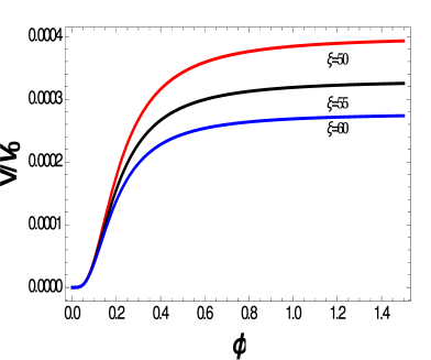
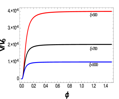
Figure 1: In both panels potential $(V(\phi)/V_{0})$ is plotted against field $\phi$, where $V_{0}=\frac{\lambda}{4}$. The left panel corresponds to small values of $\xi$, where red, black and blue lines represents $\xi=50,55$ and $60$. However, the right panel corresponds to large value of $\xi$, where red, black and blue lines represents $\xi=500,700$ and $1000$.

We plotted this newly defined potential along with the field for different values of $\xi$. Fig. 1 shows that Eq. (29) produces well-behaved inflationary potentials for arbitrary values of $\xi$.
The expressions for the slow roll parameters $\epsilon_{1}$ and $\epsilon_{2}$ from Eq. (17), Eq. (18), and Eq. (29) are obtained as

$$\epsilon_{1}=\frac{32M_{Pl}^{4}}{BM_{Pl}^{2}\lambda\phi^{6}+B\lambda\xi\phi^{8}}$$ (30)

$$\epsilon_{2}=\frac{96M_{Pl}^{4}+128M_{Pl}^{2}\xi\phi^{2}}{BM_{Pl}^{2}\lambda\phi^{6}+B\lambda\xi\phi^{8}}$$ (31)

Using these slow-roll parameters we compute the amplitude of scalar power spectrum (22), scalar spectral index (24) and tensor-to-scalar ratio (25) for $N_{k}=50$ and $60$ for various range of parameters $\xi$ and $B$. As mentioned earlier we keep $\lambda=0.14$Cheong:2021vdb ; Mohammedi:2022qqj throughout our calculations. The variation of scalar amplitude $A_{S}$ with these parameters is shown in Fig. 2

Figure 2: These contour plots represent the amplitude of scalar perturbations $A_{S}$ as function of parameters $\xi$ and $B$. the left panel is for $N_{k}$( number of e-folds)= 50 and right one is for $N_{k}=60$ .The filled pink region represents the Planck-2018 constraints on $A_{s}$.

The left side of the contour plots in Fig. 2 is for $N_{e}=50$ and the right side is for $N_{e}=60$.

We have also shown the allowed range for $A_{S}$ from Planck data Planck:2018vyg , i.e., $(2.105\pm 0.030)\times 10^{-9}$ at $68\%$CL. By imposing this constraint, we see that B varies from $7.7\times 10^{14}$ to $1.2\times 10^{15}$ for $N_{e}=50$, and from $1.2\times 10^{15}$ to $1.9\times 10^{15}$ for $N_{e}=60$, when $\xi$ decreases from $1000$ to $10$. We can conclude from Fig. 2 that the smaller values of $\xi$ requires larger values of $B$ to produce the same amplitude of scalar perturbations. However, $B$ changes by one order of magnitude to satisfy observational constraints on amplitude of scalar perturbations by increasing $N_{k}$ from $50$ to $60$.

The inclusion of the parameter, $B$, into the model helps to solve the unitarity problem of the original Higgs inflation model, in which a large value of $\xi$ is required $\left(10^{3-4}\right)$ at $\lambda=0.14$ Cheong:2021vdb ; Mohammedi:2022qqj . In this model by using a large value of $B$, we can minimize the value of $\xi$ to $\mathcal{O}\left(10\right)$.

For the range of $B$ and $\xi$ obtained using constraints on amplitude of scalar perturbations, the variation of scalar spectral index $n_{s}$ and $r$ is depicted in Fig. 3 and Fig. 4.

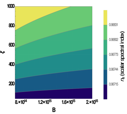
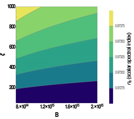
Figure 3: The contour plots represent the scalar spectral index $n_{s}$ as function of parameters $\xi$ and $B$. The number of e-foldings $N_{k}=50$ for the left panel and $N_{k}=60$ for the right one.

From these figures it can be seen that the spectral index $n_{s}$ and tensor-to-scalar ratio $r$ does not change significantly with $B$ for small values of $\xi$, and this behavior is independent of number of e-foldings. It is evident from Fig. 3 that, for constant $B$, $n_{s}$ increases with $\xi$ and the number of e-foldings. It can be seen from Fig. 4 that, for fixed $B$, $r$ decreases with increase in $\xi$ and also increase in the number of e-foldings.

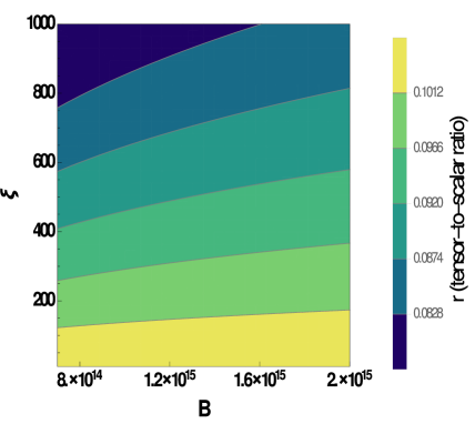
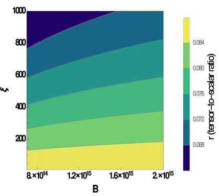
Figure 4: The contour plots represents the variation of tensor-to-scalar ratio $r$ as function of parameters $\xi$ and $B$. Again, the number of e-foldings $N_{k}=50$ for the left panel and $N_{k}=60$ for the right one.

To compute the variation of tensor-to-scalar ratio $r$ with the scalar spectral index $n_{s}$ for various values of potential parameters $B$, $\xi$ and the number of e-foldings $N_{k}$, we solve the background equations (20) and (21) numerically in terms of the independent variable $N_{e}=\ln a$. The values of the slow-roll parameters $\epsilon_{1}$ and $\epsilon_{2}$, obtained by solving background equations are then substituted in Eqs. (25,24,27) to find $r$ as a function of $n_{s}$.

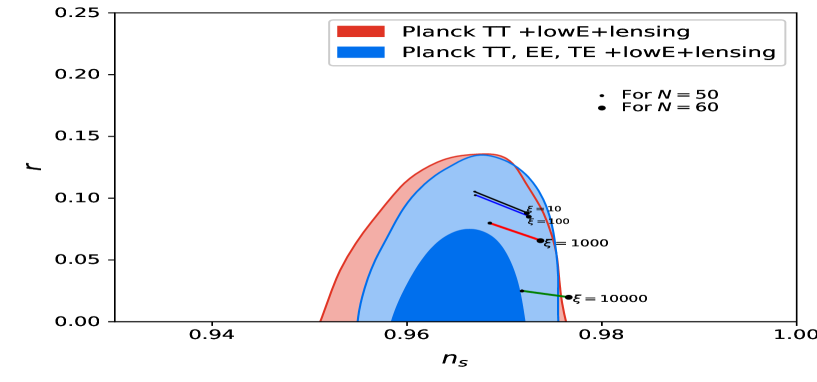
Figure 5: r vs $n_{s}$ predictions for Higgs inflation potential with non-minimally coupled tachyon field along with the joint $68\%\,\,C.L.$ and $95\%\,\,C.L.$ Planck-2018 constraints.

The variation of $r$ with respect to $n_{s}$ along with the Planck-2018 data is is shown in Fig. 5. It is evident from the figure that for the non-canonical Higgs inflation model, the spectral index $n_{s}$ and tensor-to-scalar ratio $r$ are within the $95\%$ C.L. of the Planck 2018 data for smaller values of $\xi$. As the value of $\xi$ increases, the tensor-to-scalar ratio $r$ gets smaller, while the value of the spectral index $n_{s}$ increases. The values of $n_{s}$ and $r$ for the original non-minimally coupled Higgs inflation model are independent of $\lambda$ and $\xi$, however, in our case, both observable parameters depend on the self-coupling constant $\lambda$ and the non-minimal coupling constant $\xi$.

The values of $n_{s}$ and $r$ for some selected values of $\xi$ and $N_{k}=50$ and $60$ are also shown in Table 1.

$\xi$	$N_{k}$	$n_{s}$	r
10	50	0.9669	0.1054
	60	0.9723	0.0879
$10^{2}$	50	0.9670	0.1024
	60	0.9725	0.0852
$10^{3}$	50	0.9686	0.0798
	60	0.9738	0.0656
$10^{4}$	50	0.9719	0.0249
	60	0.9766	0.0199

Table 1: The table shows the spectral index $n_{s}$ and tensor-to-scalar ratio $r$ for some selected values of $\xi$ and $N_{k}$ for constant $B=10^{15}$.

It can be seen from the table that the value of tensor-to-scalar is large for smaller values of $\xi$. To satisfy joint constraints on $r$ from Planck and BICEP3 BICEP:2021xfz i.e., $r<0.036$ at $95\%\,\,C.L.$, the value of $\xi$ should be of the order of $10^{4}$. Higgs inflation with non-canonical kinetic term yields larger values of tensor-to-scalar $r$ compared to the original Higgs inflation model.

IV Conclusions

Higgs inflation Bezrukov:2007ep , where the Higgs field of the standard model is non-minimally coupled to gravity, is one of the best suited models of inflation from Planck-2018 observations Planck:2018jri as it predicts smaller tensor-to-scalar ratio. However, this model requires large value of non-minimal coupling constant, ($\xi\sim 10^{4}$), to satisfy the observational constraints on the amplitude of scalar perturbations, This large value of $\xi$ violates unitarity, as the Higgs-Higgs scattering via graviton exchange at a scale $\Lambda=M_{Pl}/\sqrt{\xi}$ becomes strongly coupled Burgess:2009ea ; Barbon:2009ya .

In this work we consider Higgs-inflation with the non-canonical kinetic term of DBI form along with the non-minimal coupling to examine whether this can reduce the non-minimal coupling constant. As the field $\phi$ has the dimension of mass, a new parameter $B$ with dimension mass^-4 is introduced in the DBI term for dimensional consistency. To analyze the inflationary dynamics in the Einstein frame we perform a conformal rescaling of the metric field, which transforms the Jordan frame action to the minimally coupled action with a non-canonical kinetic term with modified Higgs-potential (29).

We find that the Higgs inflation exhibits different features with non-canonical kinetic term. The amplitude of the scalar perturbation depends only on the self-coupling constant $\lambda$ and the non-minimal coupling constant $\xi$ in the canonical non-minimally coupled Higgs inflation Bezrukov:2007ep , and to satisfy the cosmological and particle physics requirements at the electroweak scale, the order of $\xi$ must be $10^{3-4}$. However, for Higgs-inflation with a non-canonical kinetic term, the amplitude of the scalar perturbations $P_{s}$ is not only a function of $\lambda$ and $\xi$, but also depends on the new parameter $B$. At the electroweak scale, the self-coupling constant $\lambda$ is a function of both the Higgs mass and the mass of the top quark and has the value $0.14$ Cheong:2021vdb ; Mohammedi:2022qqj . At this value of $\lambda$, by considering a large value of $B$, we can minimize the $\xi$ at ${\mathcal{O}{(10)}}$ to satisfy the constraints on amplitude of scalar perturbations.

The variation of tensor-to-scalar ratio $r$ and the scalar spectral index $n_{s}$ along with the Joint constraints from Planck 2018 data are shown in Fig. 5 . From this, we find that the Higgs inflationary potential with a non-canonical kinetic term yields the larger value of the tensor-to-scalar ratio $r$ and satisfies the Planck-2018 constraints for $\xi\sim 10^{3}$ within $95\%\,\,C.L.$. In case of Higgs-inflation with canonical kinetic term both $n_{s}$ and $r$ depend only on the number of e-foldings , however, for Higgs-inflation with non-canonical kinetic term, these parameters also depend on field-gravity coupling constant $\xi$ and $B$. For selected values of $\xi$ and $N_{k}$ the values of $n_{s}$ and $r$ are shown in Table 1. The bounds on $r$ from from joint analysis of Planck and BICEP3 BICEP:2021xfz requires the parameter $\xi\sim 10^{4}$. Hence a non-canonical kinetic term of DBI for Higgs-inflation does not alter the observational constraints on $\xi$ significantly. This implies that the issue of unitarity violation is not resolved even after considering Higgs inflation with non-canonical kinetic term. The non-minimally coupled k-inflation with the DBI form of the kinetic energy and the potentials derived from string theory has been considered in Piao:2002nh ; Chingangbam:2004ng ; Sen:2009fkx . Although quartic potential with $\lambda=0.14$ satisfies the observational constraints for $\xi=10^{4}$, our analysis can have phenomenological implications and a detailed analysis can be performed to find the best suited values of $\lambda$ and $\xi$ from CMB and LSS observations.

References

- (1) A. H. Guth, Phys. Rev. D 23 (1981), 347-356 doi:10.1103/PhysRevD.23.347
- (2) A. D. Linde, Phys. Lett. B 129 (1983), 177-181 doi:10.1016/0370-2693(83)90837-7
- (3) A. A. Starobinsky, Phys. Lett. B 91 (1980), 99-102 doi:10.1016/0370-2693(80)90670-X
- (4) V. F. Mukhanov and G. V. Chibisov, JETP Lett. 33 (1981), 532-535
- (5) A. A. Starobinsky, Phys. Lett. B 117 (1982), 175-178 doi:10.1016/0370-2693(82)90541-X
- (6) S. W. Hawking, Phys. Lett. B 115 (1982), 295 doi:10.1016/0370-2693(82)90373-2
- (7) N. Aghanim et al. [Planck], Astron. Astrophys. 641 (2020), A6 [erratum: Astron. Astrophys. 652 (2021), C4] doi:10.1051/0004-6361/201833910 [arXiv:1807.06209 [astro-ph.CO]].
- (8) Y. Akrami et al. [Planck], Astron. Astrophys. 641 (2020), A10 doi:10.1051/0004-6361/201833887 [arXiv:1807.06211 [astro-ph.CO]].
- (9) D. H. Lyth and A. Riotto, Phys. Rept. 314 (1999), 1-146 doi:10.1016/S0370-1573(98)00128-8 [arXiv:hep-ph/9807278 [hep-ph]].
- (10) F. L. Bezrukov and M. Shaposhnikov, Phys. Lett. B 659, 703-706 (2008) doi:10.1016/j.physletb.2007.11.072 [arXiv:0710.3755 [hep-th]].
- (11) A. O. Barvinsky, A. Y. Kamenshchik and A. A. Starobinsky, JCAP 11 (2008), 021 doi:10.1088/1475-7516/2008/11/021 [arXiv:0809.2104 [hep-ph]].
- (12) F. Bezrukov, A. Magnin, M. Shaposhnikov and S. Sibiryakov, JHEP 01 (2011), 016 doi:10.1007/JHEP01(2011)016 [arXiv:1008.5157 [hep-ph]].
- (13) C. F. Steinwachs, Fundam. Theor. Phys. 199 (2020), 253-287 doi:10.1007/978-3-030-51197-5_11 [arXiv:1909.10528 [hep-ph]].
- (14) J. Rubio, Front. Astron. Space Sci. 5 (2019), 50 doi:10.3389/fspas.2018.00050 [arXiv:1807.02376 [hep-ph]].
- (15) B. Horn, MDPI Physics 2 (2020) no.3, 503-520 doi:10.3390/physics2030028 [arXiv:2007.10377 [hep-ph]].
- (16) F. Bezrukov, Class. Quant. Grav. 30 (2013), 214001 doi:10.1088/0264-9381/30/21/214001 [arXiv:1307.0708 [hep-ph]].
- (17) N. D. Birrell and P. C. W. Davies, Cambridge Univ. Press, 1984, ISBN 978-0-521-27858-4, 978-0-521-27858-4 doi:10.1017/CBO9780511622632
- (18) P. Moniz, P. Crawford and A. Barroso, Class. Quant. Grav. 7, L143-L147 (1990) doi:10.1088/0264-9381/7/7/005
- (19) A. Barroso, J. Casasayas, P. Crawford, P. Moniz and A. Nunes, Phys. Lett. B 275, 264-272 (1992) doi:10.1016/0370-2693(92)91588-Z
- (20) C. P. Burgess, H. M. Lee and M. Trott, JHEP 09, 103 (2009) doi:10.1088/1126-6708/2009/09/103 [arXiv:0902.4465 [hep-ph]].
- (21) J. L. F. Barbon and J. R. Espinosa, Phys. Rev. D 79 (2009), 081302 doi:10.1103/PhysRevD.79.081302 [arXiv:0903.0355 [hep-ph]].
- (22) C. P. Burgess, H. M. Lee and M. Trott, JHEP 07 (2010), 007 doi:10.1007/JHEP07(2010)007 [arXiv:1002.2730 [hep-ph]].
- (23) R. N. Lerner and J. McDonald, JCAP 04 (2010), 015 doi:10.1088/1475-7516/2010/04/015 [arXiv:0912.5463 [hep-ph]].
- (24) M. P. DeCross, D. I. Kaiser, A. Prabhu, C. Prescod-Weinstein and E. I. Sfakianakis, Phys. Rev. D 97 (2018) no.2, 023526 doi:10.1103/PhysRevD.97.023526 [arXiv:1510.08553 [astro-ph.CO]].
- (25) Y. Ema, R. Jinno, K. Mukaida and K. Nakayama, JCAP 02 (2017), 045 doi:10.1088/1475-7516/2017/02/045 [arXiv:1609.05209 [hep-ph]].
- (26) E. I. Sfakianakis and J. van de Vis, Phys. Rev. D 99 (2019) no.8, 083519 doi:10.1103/PhysRevD.99.083519 [arXiv:1810.01304 [hep-ph]].
- (27) Y. Ema, Phys. Lett. B 770 (2017), 403-411 doi:10.1016/j.physletb.2017.04.060 [arXiv:1701.07665 [hep-ph]].
- (28) G. F. Giudice and H. M. Lee, Phys. Lett. B 694 (2011), 294-300 doi:10.1016/j.physletb.2010.10.035 [arXiv:1010.1417 [hep-ph]].
- (29) O. Lebedev and H. M. Lee, Eur. Phys. J. C 71 (2011), 1821 doi:10.1140/epjc/s10052-011-1821-0 [arXiv:1105.2284 [hep-ph]].
- (30) G. Chakravarty, S. Mohanty and N. K. Singh, Int. J. Mod. Phys. D 23, no.4, 1450029 (2014) doi:10.1142/S0218271814500291 [arXiv:1303.3870 [astro-ph.CO]].
- (31) C. Armendariz-Picon, T. Damour and V. F. Mukhanov, Phys. Lett. B 458 (1999), 209-218 doi:10.1016/S0370-2693(99)00603-6 [arXiv:hep-th/9904075 [hep-th]].
- (32) J. Garriga and V. F. Mukhanov, Phys. Lett. B 458 (1999), 219-225 doi:10.1016/S0370-2693(99)00602-4 [arXiv:hep-th/9904176 [hep-th]].
- (33) N. D. Lambert and I. Sachs, Phys. Rev. D 67 (2003), 026005 doi:10.1103/PhysRevD.67.026005 [arXiv:hep-th/0208217 [hep-th]].
- (34) A. Sen, JHEP 12 (1999), 027 doi:10.1088/1126-6708/1999/12/027 [arXiv:hep-th/9911116 [hep-th]].
- (35) A. Sen, J. Math. Phys. 42 (2001), 2844-2853 doi:10.1063/1.1377037 [arXiv:hep-th/0010240 [hep-th]].
- (36) A. Sen, JHEP 04 (2002), 048 doi:10.1088/1126-6708/2002/04/048 [arXiv:hep-th/0203211 [hep-th]].
- (37) G. W. Gibbons, Phys. Lett. B 537, 1-4 (2002) doi:10.1016/S0370-2693(02)01881-6 [arXiv:hep-th/0204008 [hep-th]].
- (38) M. Alishahiha, E. Silverstein and D. Tong, Phys. Rev. D 70 (2004), 123505 doi:10.1103/PhysRevD.70.123505 [arXiv:hep-th/0404084 [hep-th]].
- (39) C. Ringeval, J. Phys. Conf. Ser. 203 (2010), 012056 doi:10.1088/1742-6596/203/1/012056 [arXiv:0910.2167 [astro-ph.CO]].
- (40) E. J. Copeland, S. Mizuno and M. Shaeri, Phys. Rev. D 81 (2010), 123501 doi:10.1103/PhysRevD.81.123501 [arXiv:1003.2881 [hep-th]].
- (41) V. F. Mukhanov and A. Vikman, JCAP 02 (2006), 004 doi:10.1088/1475-7516/2006/02/004 [arXiv:astro-ph/0512066 [astro-ph]].
- (42) P. Vargas Moniz, Phys. Rev. D 66, 103501 (2002) doi:10.1103/PhysRevD.66.103501
- (43) P. V. Moniz, Class. Quant. Grav. 19, L127-L134 (2002) doi:10.1088/0264-9381/19/14/102
- (44) P. Vargas Moniz, Phys. Rev. D 66, 064012 (2002) doi:10.1103/PhysRevD.66.064012
- (45) J. E. Lidsey and D. Seery, Phys. Rev. D 75 (2007), 043505 doi:10.1103/PhysRevD.75.043505 [arXiv:astro-ph/0610398 [astro-ph]].
- (46) N. C. Devi, A. Nautiyal and A. A. Sen, Phys. Rev. D 84, 103504 (2011) doi:10.1103/PhysRevD.84.103504 [arXiv:1107.4911 [astro-ph.CO]].
- (47) P. Pareek and A. Nautiyal, Phys. Rev. D 104, no.8, 083526 (2021) doi:10.1103/PhysRevD.104.083526 [arXiv:2103.01797 [astro-ph.CO]].
- (48) A. Nautiyal, Phys. Rev. D 98, no.10, 103531 (2018) doi:10.1103/PhysRevD.98.103531 [arXiv:1806.03081 [astro-ph.CO]].
- (49) T. Chiba, T. Okabe and M. Yamaguchi, Phys. Rev. D 62 (2000), 023511 doi:10.1103/PhysRevD.62.023511 [arXiv:astro-ph/9912463 [astro-ph]].
- (50) C. Armendariz-Picon, V. F. Mukhanov and P. J. Steinhardt, Phys. Rev. Lett. 85 (2000), 4438-4441 doi:10.1103/PhysRevLett.85.4438 [arXiv:astro-ph/0004134 [astro-ph]].
- (51) C. Armendariz-Picon, V. F. Mukhanov and P. J. Steinhardt, Phys. Rev. D 63 (2001), 103510 doi:10.1103/PhysRevD.63.103510 [arXiv:astro-ph/0006373 [astro-ph]].
- (52) T. Chiba, Phys. Rev. D 66 (2002), 063514 doi:10.1103/PhysRevD.66.063514 [arXiv:astro-ph/0206298 [astro-ph]].
- (53) L. P. Chimento, Phys. Rev. D 69 (2004), 123517 doi:10.1103/PhysRevD.69.123517 [arXiv:astro-ph/0311613 [astro-ph]].
- (54) L. P. Chimento and A. Feinstein, Mod. Phys. Lett. A 19 (2004), 761-768 doi:10.1142/S0217732304013507 [arXiv:astro-ph/0305007 [astro-ph]].
- (55) S. Nojiri, S. D. Odintsov and V. K. Oikonomou, Nucl. Phys. B 941 (2019), 11-27 doi:10.1016/j.nuclphysb.2019.02.008 [arXiv:1902.03669 [gr-qc]].
- (56) S. D. Odintsov, V. K. Oikonomou and F. P. Fronimos, Nucl. Phys. B 963 (2021), 115299 doi:10.1016/j.nuclphysb.2020.115299 [arXiv:2101.00660 [gr-qc]].
- (57) H. M. Lee, Eur. Phys. J. C 74, no.8, 3022 (2014) doi:10.1140/epjc/s10052-014-3022-0 [arXiv:1403.5602 [hep-ph]].
- (58) J. Lin, S. Gao, Y. Gong, Y. Lu, Z. Wang and F. Zhang, Phys. Rev. D 107, no.4, 043517 (2023) doi:10.1103/PhysRevD.107.043517 [arXiv:2111.01362 [gr-qc]].
- (59) L. N. Granda, D. F. Jimenez and W. Cardona, Astropart. Phys. 121, 102459 (2020) doi:10.1016/j.astropartphys.2020.102459 [arXiv:1911.02901 [gr-qc]].
- (60) Y. S. Piao, Q. G. Huang, X. m. Zhang and Y. Z. Zhang, Phys. Lett. B 570 (2003), 1-4 doi:10.1016/j.physletb.2003.07.047 [arXiv:hep-ph/0212219 [hep-ph]].
- (61) P. Chingangbam, S. Panda and A. Deshamukhya, JHEP 02 (2005), 052 doi:10.1088/1126-6708/2005/02/052 [arXiv:hep-th/0411210 [hep-th]].
- (62) A. A. Sen and N. C. Devi, Gen. Rel. Grav. 42 (2010), 821-838 doi:10.1007/s10714-009-0882-y [arXiv:0809.2852 [astro-ph]].
- (63) S. D. Odintsov and V. K. Oikonomou, Class. Quant. Grav. 37 (2020) no.2, 025003 doi:10.1088/1361-6382/ab5c9d [arXiv:1912.00475 [gr-qc]].
- (64) I. D. Gialamas and A. B. Lahanas, Phys. Rev. D 101 (2020) no.8, 084007 doi:10.1103/PhysRevD.101.084007 [arXiv:1911.11513 [gr-qc]].
- (65) D. Y. Cheong, S. M. Lee and S. C. Park, J. Korean Phys. Soc. 78 (2021) no.10, 897-906 doi:10.1007/s40042-021-00086-2 [arXiv:2103.00177 [hep-ph]].
- (66) N. Mohammedi, Phys. Lett. B 831 (2022), 137180 doi:10.1016/j.physletb.2022.137180 [arXiv:2202.05696 [hep-th]].
- (67) P. A. R. Ade et al. [BICEP and Keck], Phys. Rev. Lett. 127, no.15, 151301 (2021) doi:10.1103/PhysRevLett.127.151301 [arXiv:2110.00483 [astro-ph.CO]].