Equation Generator for Equation-of-Motion Coupled Cluster Assisted by Computer Algebra System

Abstract

We present an equation generator algorithm that utilizes second-quantized operators in normal order with respect to a correlated or non-correlated reference and the corresponding Wick theorem. The algorithm proposed here, written with mathematica, enables the generation of non-redundant strings of second-quantized operators that, after classification, are directly assigned to many-body term quantities used to construct the many-body Hamiltonian. We demonstrate the capabilities of the algorithm by computing the CC amplitude equations and various blocks of the equation-of-motion many-body Hamiltonian. A comprehensive description of this four-step algorithm is provided alongside concrete examples.

I Introduction

The increase in computational capabilities has led us to explore more complex wave function ansätze. As these ansätze become more complicated, deriving the corresponding algebraic equations also becomes more tedious, time-consuming, and, more importantly, subject to human errors. An important feature of many-body quantum chemistry methods is that most of them can be written in the second quantization formalism based on established commutation or anti-commutation relations between second-quantized operators. [1] In the second quantization formalism, first introduced in quantum field theory, the wave function and the operators are expressed as products of creation and annihilation operators, also known as strings. These strings can be evaluated using either (anti-)commutation rules, diagrammatic techniques, [2] or Wick’s theorem.[3] The diagrammatic approach proves to be more efficient since it avoids redundant terms.

These rules can then be programmed with the aid of symbolic algebra software, allowing us to write chains of products of these operators as tensors that can be efficiently evaluated by modern tensor contraction tools. [4, 5, 6, 7, 8, 9, 10]

In the context of coupled-cluster (CC) methods, [11, 12, 13, 14, 2] various equation generators have emerged to automate the process of deriving and implementing the corresponding equations, replacing the manual derivation and error-prone implementation in electronic structure software. In their pioneering work, Janssen and Schaefer generated and automatically implemented the open-shell CC equations by utilizing second-quantized strings. [15] In a similar vein, Li and Paldus automated the implementation of spin-adapted open-shell CC equations, with the added benefit of utilizing the unitary group formalism that allows for the efficient handling of low-spin states. [16] In 2001, Kállay and Surján proposed a general-order CC code by combining diagrammatic many-body perturbation theory and string-based configuration interaction. [17] In such a way, the CC equations were written in terms of diagrams and stored as strings. This technique was then generalized to state-specific multireference CC, [18] excited states computed within the linear response formalism,[19] and approximate treatment of higher excitations. [20]

Adopting the same design philosophy as Janssen and Schaefer, Hirata implemented the Tensor Contraction Engine (tce) [21, 22, 23, 24] that performs the manipulation of second-quantized operators and the generation of the computer code. The main distinction is that tce takes advantage of spin, spatial, and index permutation symmetries at every stage of the calculations, reducing the computational cost and storage requirement. Later on, Hirata also developed an equation generator for equation-of-motion (EOM) CC [25, 26, 27, 28, 29, 30, 31] for neutral excitations (EE-EOM-CC), [25, 26, 27, 28] ionization potentials (IP-EOM-CC),[32, 33, 34, 35, 36, 34] and electron affinities (EA-EOM-CC). [11, 37, 38, 39] Hanrath et al. proposed an improved version of tce by implementing the matrix-matrix multiplication-based antisymmetric tensor contraction for general CC. [40, 41] Meanwhile, Kong et al. developed the EOM version of state-specific multireference CC together with the automated implementation of such complicated equations.[42] This was later generalized to arbitrary order. [43, 44, 45, 46] Likewise, Shiozaki implemented explicitly-correlated versions of CC in a similar way. [47, 48]

More recently appeared (i) the Symbolic Manipulation Interpreter for Theoretical cHemistry (smith3)[49] for complete active space methods that implies partial contractions of second-quantized operators, (ii) p^†q developed by Rubin and DePrince III [50] that combines C++ and python for proof-of-concept implementation of many-body quantum chemistry methods, and (iii) wick&d [51] that presents a strategy to evaluate Mukherjee’s [52] and Kutzelnigg’s [53] version of Wick’s theorem in the case of an arbitrary number of orbital subspaces. Each of the above programs is a clear example of the progress that has been achieved in the last three decades with respect to equation generators in quantum chemistry.

The aim of the present paper is to describe a four-step algorithm based on Wick’s theorem to obtain the working equations of EE-EOM-CC, IP-EOM-CC, EA-EOM-CC, as well as other quantities of interest. In particular, the direct way of obtaining intermediates facilitates the comparison between many-body perturbation theory and CC methods. [54, 55, 56, 57, 58] The present algorithm is implemented with the computer algebra system, mathematica, [59] in order to be able to generate and manipulate the equations in a user-friendly way.

This article is organized as follows. Section II gathers all theoretical details. In particular, Sec. II.1 describes Wick’s theorem and the concept of normal ordering. Then, in Secs. II.2 and II.3, we report the main theoretical details behind the CC and EOM-CC equations, respectively. Finally, in Sec. III, we provide a detailed description of our algorithm. Our conclusions are drawn in Sec. IV.

II Theory

II.1 Normal ordering and Wick’s theorem

Our goal is to derive automatically the EOM-CC working equations which is a matrix eigenvalue problem. Each element of the EOM-CC effective Hamiltonian is an expectation value formed by products of operators. (We shall discuss this point in more detail later in this section). An efficient way to evaluate these products of operators is via their second-quantized form. [60, 61, 62]

As a starting point, let us introduce the reference state which is represented as a single determinant

$$\ket*{0}=\ket*{ijk\cdots}=\hat{i}^{{\dagger}}\hat{j}^{{\dagger}}\hat{k}^{{\dagger}}\cdots\ket*{}.$$ (1)

obtained by acting on the physical (or true) vacuum $\ket*{}$ with creation operators $\hat{i}^{{\dagger}}$, $\hat{j}^{{\dagger}}$, $\hat{k}^{{\dagger}}$, $\ldots$. This reference state $\ket*{0}$, typically taken as the Hartree-Fock (HF) ground-state determinant, can be used as an alternative vacuum, named Fermi vacuum. [14, 2] One property of the Fermi vacuum is that one can redefine the creation operators relative to it as particles ($\hat{a}^{{\dagger}}$, $\hat{b}^{{\dagger}}$, $\hat{c}^{{\dagger}}$, $\ldots$) and holes ($\hat{i}$, $\hat{j}$, $\hat{k}$, $\ldots$).[63, 64] The particle creation operators create particle states above the Fermi level while the hole creation operators remove particle states below the Fermi level (particle-hole formalism). Because one cannot annihilate a hole or remove a particle in the Fermi vacuum, we have $\hat{i}^{{\dagger}}\ket*{0}=0$ and $\hat{a}\ket*{0}=0$.

It is also possible to define “neutral” excited determinants by operating the same number of particle and hole operators onto the Fermi vacuum:

$$\hat{a}^{{\dagger}}\hat{b}^{{\dagger}}\hat{c}^{{\dagger}}\cdots\hat{k}\hat{j}\hat{i}\ket*{0}=\ket*{\Phi_{ijk\cdots}^{abc\cdots}}.$$ (2)

In such a way, it is also possible to define “charged” excited determinants when the number of particles and holes are different. For example, ionized and electron-attached determinants can be represented respectively, as follows

$$\hat{a}^{{\dagger}}\hat{j}\hat{i}\ket{0} =\ket*{\Phi_{ij}^{a}},$$ (3)

$$\hat{a}^{{\dagger}}\hat{b}^{{\dagger}}\hat{i}\ket{0} =\ket*{\Phi_{i}^{ab}}.$$

To preserve the antisymmetry of the electronic wave function, the second-quantized fermionic operators fulfill anti-commutation rules

$$\hat{p}\hat{q}+\hat{q}\hat{p} =0,$$ (4)

$$\hat{p}^{{\dagger}}\hat{q}^{{\dagger}}+\hat{q}^{{\dagger}}\hat{p}^{{\dagger}} =0,$$

$$\hat{p}^{{\dagger}}\hat{q}+\hat{q}^{{\dagger}}\hat{p} =\delta_{pq},$$

where $\hat{p}$, $\hat{q}$, $\hat{r}$, $\ldots$ are arbitrary operators that can be either hole or particle operators, and $\delta_{pq}$ is a Kronecker delta.

Besides the anti-commutation rules defined in Eq. (4), there is another powerful “bookkeeping system” called normal ordering, [65] that consists of placing all the creation operators to the left and all annihilation operators to the right. Therefore, applying the Fermi vacuum on a normal-ordered string yield zero. At this stage, it is convenient to introduce a more compact notation to take full advantage of this bookkeeping system. To do so, we define the contraction of arbitrary operators

$$\contraction{}{\hat{p}^{{\dagger}}}{}{\hat{q}}\hat{p}^{{\dagger}}\hat{q}=\hat{p}^{{\dagger}}\hat{q}-\{\hat{p}^{{\dagger}}\hat{q}\}=\hat{p}^{{\dagger}}\hat{q}+\hat{q}\hat{p}^{{\dagger}}=\delta_{pq},$$ (5)

where $\{\hat{p}^{{\dagger}}\hat{q}\}$ means that the product $\hat{p}^{{\dagger}}\hat{q}$ is normal ordered with respect the Fermi vacuum. By definition, the only non-zero contractions in Eq. (5) are

$$\contraction{}{\hat{a}}{}{\hat{b}}\hat{a}\hat{b}^{\dagger} =\delta_{ab},$$ (6)

$$\contraction{}{\hat{i}}{{}^{\dagger}}{\hat{j}}\hat{i}^{\dagger}\hat{j} =\delta_{ij}.$$

When a product of second-quantized operators is normal-ordered, we name it a normal product.

We are now in a position to introduce the generalized Wick theorem stating that a product of creation and annihilation operators is equal to their normal product plus the sum of all possible contractions. [2] For example, applying this theorem to a given string of normal-ordered operators (which is typically what one has to do to derive the EOM-CC equations), one gets

$$\{\hat{A}\}\{\hat{B}\}\{\hat{C}\}\cdots=\{\hat{A}\hat{B}\hat{C}\cdots\}+\sum_{\text{singles}}\{\contraction{}{\hat{A}}{\hat{B}\hat{C}}{\cdots}\hat{A}\hat{B}\hat{C}\cdots\cdots\}+\sum_{\text{doubles}}\{\contraction{}{\hat{A}}{\hat{B}\hat{C}}{\cdots}\contraction[2ex]{\hat{A}}{\hat{B}}{\hat{C}\hat{C}}{\cdots}\hat{A}\hat{B}\hat{C}\cdots\cdots\}+\cdots+\sum_{\text{fully contracted}}\{\contraction{}{\hat{A}}{\hat{B}\hat{C}}{\cdots}\contraction[2ex]{\hat{A}}{\hat{B}}{\hat{C}\hat{C}}{\cdots}\contraction[3ex]{\hat{A}\hat{B}}{\hat{C}}{\cdots}{\cdots}\hat{A}\hat{B}\hat{C}\cdots\cdots\},$$ (7)

where the first term on the right-hand side is the normal product, the second term contains all the single contractions, the third contains all double contractions, and the last sum gathers the so-called fully contracted terms. The key feature of this theorem is that, if we evaluate the Fermi vacuum expectation value associated with Eq. (7), the only non-zero terms correspond to the fully contracted ones, i.e.,

$$\matrixelement{0}{\{\hat{A}\}\{\hat{B}\}\{\hat{C}\}\cdots}{0}=\sum_{\text{fully contracted}}\matrixelement{0}{\{\contraction{}{\hat{A}}{\hat{B}\hat{C}}{\cdots}\contraction[2ex]{\hat{A}}{\hat{B}}{\hat{C}\hat{C}}{\cdots}\contraction[3ex]{\hat{A}\hat{B}}{\hat{C}}{\cdots}{\cdots}\hat{A}\hat{B}\hat{C}\cdots\cdots\}}{0}$$ (8)

To have a consistent nomenclature, the products of second-quantized operators $\{\hat{A}\}\{\hat{B}\}\{\hat{C}\}$ are called strings, and each operator $\{\hat{A}\}$ is called a sub-string.

II.2 Coupled-cluster equations

To derive the CC equations, one first starts with the definition of the CC wave function which is an exponential parametrization applied to a reference determinant [66, 67]

$$\ket*{\Psi^{(0)}}=e^{\hat{T}}\ket{0},$$ (9)

where $\Psi^{(0)}$ is the CC ground-state wave function and

$$\hat{T}=\sum_{n=1}^{N}\hat{T}_{n}$$ (10)

is the cluster operator with

$$\hat{T}_{n}=\frac{1}{(n!)^{2}}\sum_{ijk\cdots}\sum_{abc\cdots}t_{ijk\cdots}^{abc\cdots}\{\hat{a}^{{\dagger}}\hat{i}\hat{b}^{{\dagger}}\hat{j}\hat{c}^{{\dagger}}\hat{k}\cdots\},$$ (11)

where $t_{ijk\cdots}^{abc\cdots}$ are the antisymmetric cluster amplitudes and the indices $i$, $j$, $k$, $\ldots$ indicate occupied spinorbitals in the reference configuration, while $a$, $b$, $c$, $\ldots$ are unoccupied spinorbitals. In general, $\hat{T}_{n}$ produces $n$-fold excited $N$-electron determinants of the form $\ket*{\Phi_{ijk\cdots}^{abc\cdots}}$ (with $n\leq N$). It is worth mentioning here that the excitation operators do commute with each other, i.e., $\commutator*{\hat{T}_{n}}{\hat{T}_{m}}=0$.

The electronic Schrödinger equation associated with the CC wave function is

$$\hat{H}\ket*{\Psi^{(0)}}=E^{(0)}\ket*{\Psi^{(0)}},$$ (12)

where $E^{(0)}$ is the CC ground-state electronic energy, and $\hat{H}$ is the electronic Hamiltonian, which can be expressed in second-quantized form as follows:

$$\hat{H}=\sum_{pq}h_{q}^{p}\hat{p}^{{\dagger}}\hat{q}+\frac{1}{4}\sum_{pqrs}v_{rs}^{pq}\hat{p}^{{\dagger}}\hat{q}^{{\dagger}}\hat{s}\hat{r},$$ (13)

where the indices $p$, $q$, $r$, and $s$ indicate arbitrary (i.e., occupied or virtual) spinorbitals. The matrix element $h_{q}^{p}$ is the sum of the kinetic and nuclear attraction components. The electronic repulsion is accounted for by the (antisymmetrized) two-electron integrals $v_{rs}^{pq}$. Because one is usually interested in the correlated part of the Hamiltonian, it is common practice to divide it as

$$\hat{H}=\hat{H}_{\text{N}}+\matrixelement{0}{\hat{H}}{0},$$ (14)

where the first term

$$\hat{H}_{\text{N}}=\hat{F}_{\text{N}}+\hat{V}_{\text{N}}=\sum_{pq}f_{q}^{p}\{\hat{p}^{{\dagger}}\hat{q}\}+\frac{1}{4}\sum_{pqrs}v_{rs}^{pq}\{\hat{p}^{{\dagger}}\hat{q}^{{\dagger}}\hat{s}\hat{r}\}$$ (15)

is the normal-ordered Hamiltonian (where $f_{q}^{p}$ is an element of the Fock matrix) that corresponds to fluctuations (i.e., correlation) with respect to the second term that represents the reference energy $E_{0}=\bra{0}\hat{H}\ket{0}$. It is worth emphasizing that $\hat{H}_{\text{N}}$ do not commute with $\hat{T}_{n}$, i.e., $\commutator*{\hat{T}_{n}}{\hat{H}_{\text{N}}}\neq 0$.

Thanks to the exponential ansatz of the CC wave function, Eq. (9), and the introduction of the following CC effective Hamiltonian via a similarity transformation

$$\bar{H}^{\text{st}}=e^{-\hat{T}}\hat{H}_{\text{N}}e^{\hat{T}},$$ (16)

where the superindex “st” stands for “similarity-transformed”. Then, one can recast the Schrödinger equation as

$$\bar{H}^{\text{st}}\ket{0}=\Delta E^{(0)}\ket{0}.$$ (17)

where $\Delta E^{(0)}=E^{(0)}-E_{0}$ is the CC ground-state correlation energy obtained via projection

$$\matrixelement*{0}{\bar{H}^{\text{st}}}{0}=\Delta E^{(0)},$$ (18)

while

$$\matrixelement*{\Phi_{ijk\cdots}^{abc\cdots}}{\bar{H}^{\text{st}}}{0}=0$$ (19)

are the so-called amplitude equations, a set of non-linear equations where the unknowns are the cluster amplitudes $t_{ijk\cdots}^{abc\cdots}$.

To evaluate efficiently Eq. (19), one usually relies on the Baker-Campbell-Hausdorff expansion [68, 69] of the similarity-transformed Hamiltonian,

$$\bar{H}^{\text{st}}=\hat{H}_{\text{N}}+\commutator{\hat{H}_{\text{N}}}{\hat{T}}+\frac{1}{2!}\commutator{\commutator{\hat{H}_{\text{N}}}{\hat{T}}}{\hat{T}}+\frac{1}{3!}\commutator{\commutator{\commutator{\hat{H}_{\text{N}}}{\hat{T}}}{\hat{T}}}{\hat{T}}+\frac{1}{4!}\commutator{\commutator{\commutator{\commutator{\hat{H}_{\text{N}}}{\hat{T}}}{\hat{T}}}{\hat{T}}}{\hat{T}},$$ (20)

a series of nested commutators between $\hat{H}_{\text{N}}$ and $\hat{T}$ that naturally terminates at the four-fold commutator thanks to the two-body nature of the electronic Hamiltonian.

Then, using Wick’s theorem [see Eq. (7)], one can establish that the non-zero terms in Eq. (20) involve $\hat{H}_{\text{N}}$ as the left-most operator contracted with at most four $\hat{T}$ operators, i.e.,

$$\bar{H}^{\text{st}}=\hat{H}_{\text{N}}+\contraction{}{\hat{H}_{\text{N}}}{}{\hat{T}}\hat{H}_{\text{N}}\hat{T}+\frac{1}{2}\contraction{}{\hat{H}_{\text{N}}}{}{\hat{T}}\contraction{}{\hat{H}_{\text{N}}}{\hat{T}}{\hat{T}}\hat{H}_{\text{N}}\hat{T}\hat{T}+\frac{1}{3!}\contraction{}{\hat{H}_{\text{N}}}{}{\hat{T}}\contraction{}{\hat{H}_{\text{N}}}{\hat{T}}{\hat{T}}\contraction{}{\hat{H}_{\text{N}}}{\hat{T}}{\hat{T}\hat{T}\hat{T}}\hat{H}_{\text{N}}\hat{T}\hat{T}\hat{T}+\frac{1}{4!}\contraction{}{\hat{H}_{\text{N}}}{}{\hat{T}}\contraction{}{\hat{H}_{\text{N}}}{\hat{T}}{\hat{T}}\contraction{}{\hat{H}_{\text{N}}}{\hat{T}}{\hat{T}\hat{T}\hat{T}}\contraction{}{\hat{H}_{\text{N}}}{\hat{T}}{\hat{T}\hat{T}\hat{T}\hat{T}\hat{T}}\hat{H}_{\text{N}}\hat{T}\hat{T}\hat{T}\hat{T},$$ (21)

where the multi-leg symbol indicates that $\hat{H}_{\text{N}}$ must be contracted at least once with each $\hat{T}$. Hence, $\hat{H}_{\text{N}}$ is said to be connected as it does not include disconnected terms of the form $\contraction{}{\hat{H}_{\text{N}}}{}{\hat{T}}\contraction{}{\hat{H}_{\text{N}}}{\hat{T}}{\hat{T}}\hat{H}_{\text{N}}\hat{T}\hat{T}\hat{T}$.

If one introduces the right-hand side of Eq. (21) in Eqs. (18) and (19), one gets

$$\matrixelement{0}{\left(\hat{H}_{\text{N}}e^{\hat{T}}\right)_{C}}{0}=\Delta E^{(0)},$$ (22a)

$$\matrixelement{\Phi_{ijk\cdots}^{abc\cdots}}{\left(\hat{H}_{\text{N}}e^{\hat{T}}\right)_{C}}{0}=0.$$ (22b)

where the subindex $C$ stands for connected. Since one only deals with the connected terms, the algebraic form of Eqs. (22a) and (22b) is simpler than Eqs. (18) and (19).

II.3 Equation-of-motion coupled-cluster equations

Having explained how to derive the CC equations, next, we shift our attention to the EOM-CC equations. [29, 30, 31, 25] As a starting point, let us consider the Schrödinger equation for a target excited state $\Psi^{(k)}$, i.e.,

$$\hat{H}_{\text{N}}\ket*{\Psi^{(k)}}=\Delta E^{(k)}\ket*{\Psi^{(k)}},$$ (23)

with $\Delta E^{(k)}=E^{(k)}-E_{0}$. One way to access this target state is by transforming the initial state described by Eq. (17) via an excitation operator of the form

$$\hat{\mathcal{R}}^{(k)}\ket*{\Psi^{(0)}}=\ket*{\Psi^{(k)}}$$ (24)

If one wants to access neutral excited states, one must rely on the excitation energy (EE) operator

$$\hat{\mathcal{R}}^{(k)}=\hat{1}+\hat{\mathcal{R}}_{1}^{(k)}+\hat{\mathcal{R}}_{2}^{(k)}+\cdots$$ (25)

with

$$\hat{\mathcal{R}}_{1}^{(k)}=\sum_{i}\sum_{a}r_{i}^{a}\{\hat{a}^{{\dagger}}\hat{i}\},$$ (26a)

$$\hat{\mathcal{R}}_{2}^{(k)}=\frac{1}{4}\sum_{ij}\sum_{ab}r_{ij}^{ab}\{\hat{a}^{{\dagger}}\hat{i}\hat{b}^{{\dagger}}\hat{j}\},$$ (26b)

$$\vdots$$

where $\hat{\mathcal{R}}_{n}^{(k)}$ is an excitation operator of degree $n$ for the state $k$ associated with the EOM-CC amplitudes $r_{ab\cdots}^{ij\cdots}$. (Here, for the sake of simplicity, we have omitted the $k$-dependence of the amplitudes.)

After several transformations, the Schrödinger equation for the target excited state [see Eq. (23)] can be recast as

$$\commutator{\bar{H}^{\text{st}}}{\hat{\mathcal{R}}^{(k)}}\ket{0}=\Omega_{k}\hat{\mathcal{R}}^{(k)}\ket{0}.$$ (27)

where $\Omega_{k}=E^{(k)}-E^{(0)}$ is the excitation energy associated with the $k$th excited state. Defining the normal-ordered similarity-transformed Hamiltonian, $\bar{H}_{\text{N}}^{\text{st}}={\color[rgb]{0,0,0}\bar{H}^{\text{st}}}-E^{(0)}$, the commutator in Eq. (27) can be further simplified as

$$\left(\bar{H}_{\text{N}}^{\text{st}}\hat{\mathcal{R}}^{(k)}\right)_{C}\ket{0}=\Omega_{k}\hat{\mathcal{R}}^{(k)}\ket{0}.$$ (28)

The excitation energies are then directly computed by projecting Eq. (28) in a determinant basis truncated at a given excitation degree, which is equivalent to truncate $\hat{\mathcal{R}}^{(k)}$.

Introducing the simplified notation, $\ket{\Phi_{i}^{a}}\equiv\ket{S}$, $\ket{\Phi_{ij}^{ab}}\equiv\ket{D}$, $\ldots$, the EOM-CC linear eigenvalue problem has the following form:

$$\boldsymbol{\mathcal{\bar{H}}}\mathbb{r}_{k}=\Omega_{k}\mathbb{r}_{k}\mbox{\quad$\Rightarrow$\quad}\begin{pmatrix}\bra{S}\bar{H}_{\text{N}}^{\text{st}}\ket{S}&\bra{S}\bar{H}_{\text{N}}^{\text{st}}\ket{D}&\cdots\\ \bra{D}\bar{H}_{\text{N}}^{\text{st}}\ket{S}&\bra{D}\bar{H}_{\text{N}}^{\text{st}}\ket{D}&\cdots\\ \vdots&\vdots&\ddots\end{pmatrix}\begin{pmatrix}r_{i}^{a}&\\ r_{ij}^{ab}&\\ \vdots&\end{pmatrix}=\Omega_{k}\begin{pmatrix}r_{i}^{a}&\\ r_{ij}^{ab}&\\ \vdots&\end{pmatrix}.$$ (29)

Here, $\boldsymbol{\mathcal{\bar{H}}}$ represents the EOM-CC matrix, while $\mathbb{r}_{k}$ and $\Omega_{k}$ are the corresponding eigenvector and eigenvalue, respectively. The non-Hermitian nature of this eigenvalue problem necessitates the computation of each block of the matrix. Furthermore, this non-Hermitian characteristic indicates that $\boldsymbol{\mathcal{\bar{H}}}$ is also associated with left eigenfunctions $\bra*{\Psi^{(0)}}\hat{\mathcal{L}}_{1}^{(k)}=\bra*{\Psi^{(k)}}$ stemming from the following Schrödinger equation $\bra*{\Psi^{(k)}}\hat{H}_{\text{N}}=\bra*{\Psi^{(k)}}\Delta E^{(k)}$, where $\hat{\mathcal{L}}^{(k)}=\hat{1}+\hat{\mathcal{L}}_{1}^{(k)}+\hat{\mathcal{L}}_{2}^{(k)}+\cdots$ is a de-excitation operator, such that $\hat{\mathcal{L}}_{1}^{(1)}=\sum_{i}\sum_{a}l_{i}^{a}\{\hat{i}^{{\dagger}}\hat{a}\}$, for example. This results in the following left-hand side eigenvalue equation

$$\mathbb{l}_{k}\boldsymbol{\mathcal{\bar{H}}}=\mathbb{l}_{k}\Omega_{k}^{*}$$ (30)

The two sets of eigenfunctions can be normalized to satisfy $\bra*{\Psi^{(0)}}\hat{\mathcal{L}}_{1}^{(l)}\hat{\mathcal{R}}^{(k)}\ket*{\Psi^{(0)}}=\delta_{lk}$.

Following the same procedure, one can also obtain the EOM-CC equations for the ionized and electron-attached states, just by changing the definition of the operator $\hat{\mathcal{R}}^{(k)}$ in Eq. (26). For example, removing one or two particles, one gets IP-EOM-CC and DIP-EOM-CC, [70, 71, 72, 73, 74] respectively, while removing one or two holes yields EA-EOM-CC and DEA-EOM-CC, [73, 74] respectively.

II.4 Many-body Hamiltonian

When one computes the expectation value associated with a given block of the EOM-CC matrix $\boldsymbol{\mathcal{\bar{H}}}$ [see Eq. (29)], redundant terms are generated. One way to avoid redundancies is to rely on the many-body representation of the EOM-CC effective Hamiltonian [75, 76, 77, 78]

$$\bar{H}_{\text{N}}^{\text{mb}}=\sum_{pq}\chi_{q}^{p}\{\hat{p}^{{\dagger}}\hat{q}\}+\sum_{pqrs}\chi_{rs}^{pq}\{\hat{p}^{{\dagger}}\hat{q}^{{\dagger}}\hat{s}\hat{r}\}+\chi_{stu}^{pqr}\{\hat{p}^{{\dagger}}\hat{q}^{{\dagger}}\hat{r}^{{\dagger}}\hat{u}\hat{t}\hat{s}\}+\cdots,$$ (31)

where $\chi_{q}^{p}$, $\chi_{rs}^{pq}$, $\chi_{stu}^{pqr}$ are one-, two-, and three-body terms respectively. The superindex “mb” stands for “many-body”. Note that $\bar{H}_{\text{N}}^{\text{mb}}$ and $\bar{H}_{\text{N}}^{\text{st}}$ are exactly the same quantity; the labels “mb” and “st” are here to indicate the type of expansion.

The many-body terms $\{\chi_{stu\cdots}^{pqr\cdots}\}$ are usually represented through diagrammatic techniques. [2] In the present work though, we are interested in describing them within the second quantization formalism. To achieve this, we take as an example the block $\bra{D}\bar{H}_{\text{N}}^{\text{mb}}\ket{S}$ and the many-body Hamiltonian defined in Eq. (31) to obtain

$$\bra{\Phi_{ij}^{ab}}\bar{H}_{\text{N}}^{\text{mb}}\ket{\Phi_{k}^{c}}=\sum_{pq}\chi_{q}^{p}\bra{0}\{\hat{i}^{{\dagger}}\hat{j}^{{\dagger}}\hat{b}\hat{a}\}\{\hat{p}^{{\dagger}}\hat{q}\}\{\hat{c}^{{\dagger}}\hat{k}\}\ket{0}+\sum_{pqrs}\chi_{rs}^{pq}\bra{0}\{\hat{i}^{{\dagger}}\hat{j}^{{\dagger}}\hat{b}\hat{a}\}\{\hat{p}^{{\dagger}}\hat{q}^{{\dagger}}\hat{s}\hat{r}\}\{\hat{c}^{{\dagger}}\hat{k}\}\ket{0}\\ +\sum_{pqrstu}\chi_{stu}^{pqr}\bra{0}\{\hat{i}^{{\dagger}}\hat{j}^{{\dagger}}\hat{b}\hat{a}\}\{\hat{p}^{{\dagger}}\hat{q}^{{\dagger}}\hat{r}^{{\dagger}}\hat{u}\hat{t}\hat{s}\}\{\hat{c}^{{\dagger}}\hat{k}\}\ket{0}.$$ (32)

Equation (32) effectively terminates at the three-body level since higher-order terms produce partial contractions which are zero with respect to the Fermi vacuum.

By applying Wick’s theorem to Eq. (32) and taking advantage of the antisymmetric permutation of the many-body terms, one gets

$$\matrixelement{\Phi_{ij}^{ab}}{\bar{H}_{\text{N}}^{\text{mb}}}{\Phi_{k}^{c}}=\delta_{jk}\delta_{bc}\chi_{i}^{a}-\delta_{ik}\delta_{bc}\chi_{j}^{a}-\delta_{jk}\delta_{ac}\chi_{i}^{b}+\delta_{jk}\delta_{ac}\chi_{j}^{b}-\delta_{bc}\chi_{ij}^{ak}-\delta_{jk}\chi_{ci}^{ab}+\delta_{ik}\chi_{cj}^{ab}+\delta_{ac}\chi_{ij}^{bk}+\chi_{ijc}^{abk}.$$ (33)

Since $\bar{H}_{\text{N}}^{\text{mb}}=\bar{H}_{\text{N}}^{\text{st}}$, the block $\bra{D}\bar{H}_{\text{N}}^{\text{mb}}\ket{S}$ can be naturally written in terms of $\hat{T}$, $\hat{F}_{\text{N}}$, and $\hat{V}_{\text{N}}$. To illustrate this, we consider the general many-body term

$$\chi_{ij\cdots cd\cdots}^{ab\cdots kl\cdots}=\bra{\Phi_{ij\cdots}^{ab\cdots}}\bar{H}_{\text{N}}^{\text{st}}\ket{\Phi_{kl\cdots}^{cd\cdots}}_{iC},$$ (34)

where the subscript $iC$ represents “internal contractions”, i.e., contractions occurring exclusively between $\bra{\Phi_{ij\cdots}^{ab\cdots}}$ and $\bar{H}_{\text{N}}$, as well as $\bar{H}_{\text{N}}$ and $\ket{\Phi_{kl\cdots}^{cd\cdots}}$. Notably, contractions between $\bra{\Phi_{ij\cdots}^{ab\cdots}}$ and $\ket{\Phi_{kl\cdots}^{cd\cdots}}$ are not allowed.

Taking into account Eq. (34) and the non-zero matrix elements of $\chi_{ij}^{ak}$, one gets

$$\chi_{ij}^{ak}=\matrixelement{\Phi_{ij}^{a}}{\quantity(\hat{V}_{\text{N}}+\hat{T}_{1}\hat{V}_{\text{N}}+\hat{F}_{\text{N}}\hat{T}_{2}+\hat{V}_{\text{N}}\hat{T}_{2}+\frac{1}{2!}\hat{V}_{\text{N}}\hat{T}_{1}^{2}+\hat{V}_{\text{N}}\hat{T}_{1}\hat{T}_{2}+\frac{1}{3!}\hat{V}_{\text{N}}\hat{T}_{1}^{3})_{C}}{\Phi_{k}}_{iC}.$$ (35)

Applying the same procedure for $\chi_{ci}^{ab}$ and $\chi_{ijc}^{abk}$, we obtain

$$\chi_{ic}^{ab}=\matrixelement{\Phi_{i}^{ab}}{\quantity(\hat{V}_{\text{N}}+\hat{T}_{1}\hat{V}_{\text{N}}+\hat{F}_{\text{N}}\hat{T}_{2}+\hat{V}_{\text{N}}\hat{T}_{2}+\frac{1}{2!}\hat{V}_{\text{N}}\hat{T}_{1}^{2}+\hat{V}_{\text{N}}\hat{T}_{1}\hat{T}_{2}+\frac{1}{3!}\hat{V}_{\text{N}}\hat{T}_{1}^{3})_{C}}{\Phi^{c}}_{iC},$$ (36)

$$\chi_{ijc}^{abk}=\matrixelement{\Phi_{ij}^{ab}}{\left(\hat{V}_{\text{N}}\hat{T}_{2}\right)_{C}}{\Phi_{k}^{c}}_{iC}.$$ (37)

The one-body terms in Eq. (33) are defined as follows

$$\chi_{i}^{a}=\matrixelement{\Phi_{i}^{a}}{\quantity[\hat{H}_{\text{N}}\quantity(1+\hat{T}_{1}+\hat{T}_{2}+\frac{\hat{T}_{1}^{2}}{2}+\hat{T}_{1}\hat{T}_{2}+\frac{\hat{T}_{1}^{3}}{3!})]_{C}}{0},$$ (38)

which is identical to the CCS amplitude equations. Consequently, all the one-body terms are zero in Eq. (33). This is also true for the many-body terms $\chi_{ij}^{ab}$ for CCSD, $\chi_{ijk}^{abc}$ for CCSDT, and so on.

Setting the one-body terms equal to zero in Eq. (38), we have

$$\bra{\Phi_{ij}^{ab}}\bar{H}_{\text{N}}^{\text{mb}}\ket{\Phi_{k}^{c}}=-\delta_{bc}\chi_{ij}^{ak}-\delta_{jk}\chi_{ci}^{ab}+\delta_{ik}\chi_{cj}^{ab}+\delta_{ac}\chi_{ij}^{bk}+\chi_{ijc}^{abk}.$$ (39)

It is possible to obtain the rest of the many-body terms in Eq. (39) by substituting the indices of $\chi_{ij}^{ab}$, $\chi_{ci}^{ab}$, and $\chi_{ijc}^{abk}$. These replacements are restricted to indices of the same category: hole-creation ($i,j$), particle-annihilation ($a,b$), hole-annihilation ($k$), and particle-creation ($c$).

To obtain the block $\bra{\Phi_{ij}^{ab}}\bar{H}_{\text{N}}^{\text{mb}}\ket{\Phi_{k}^{c}}$ in a compact and non-redundant form, we rely on Eqs. (35), (36), and (37) to define the many-body terms and Eq. (39) to define the blocks in terms of these many-body terms. Finally, to generate the entire eigenvalue equations for EE-EOM-CCSD, one must repeat the same procedure for the blocks $\bra{\Phi_{i}^{a}}\bar{H}_{\text{N}}^{\text{st}}\ket{\Phi_{k}^{c}}$, $\bra{\Phi_{i}^{a}}\bar{H}_{\text{N}}^{\text{st}}\ket{\Phi_{kl}^{cd}}$, $\bra{\Phi_{ij}^{ab}}\bar{H}_{\text{N}}^{\text{st}}\ket{\Phi_{kl}^{cd}}$, and then remove the redundant many-body terms.

III EOM-CC equation generator

In this section, we describe the algorithm we have written with mathematica to automatically derive the working equations of EOM-CC. Although the program is not optimized for efficiency, our goal is to obtain the working equations in terms of the many-body terms by using straightforward input quantities. First of all, we adapt the index notations in order to have more suitable and general notations to obtain the EOM-CC equations up to fourth order. For the operators belonging to the bra and the ket, instead of using $\hat{a}^{{\dagger}}$, $\hat{b}^{{\dagger}}$, $\ldots$, $\hat{i}$, $\hat{j}$, $\ldots$, we use $\hat{p}^{{\dagger}}_{1}$, $\hat{p}^{{\dagger}}_{2}$, $\ldots$, $\hat{h}_{1}$, $\hat{h}_{2}$, $\ldots$. For the particles/holes that play the role of dummy indices in the cluster operator $\hat{T}$, instead of using $\hat{e}^{{\dagger}}$, $\hat{f}^{{\dagger}}$, $\ldots$, $\hat{m}$, $\hat{n}$, $\ldots$, we use $\hat{o}^{{\dagger}}_{1}$, $\hat{o}^{{\dagger}}_{2}$, $\ldots$, $\hat{v}_{1}$, $\hat{v}_{2}$, $\ldots$, where the notation of ${o}$ and ${v}$ refers to occupied and virtual, respectively. Finally, for the arbitrary indexes that could be either particle or hole [like the Hamiltonian in Eq. (14)], we switch from $\hat{p}^{{\dagger}}$, $\hat{q}^{{\dagger}}$, $\hat{r}$, $\hat{s}$ to $\hat{q}^{{\dagger}}_{1}$, $\hat{q}^{{\dagger}}_{2}$, $\hat{q}_{3}$, $\hat{q}_{4}$.

Thanks to this change in notation, we can now describe the four-step algorithm that we use to derive the EOM-CC equations. Each step of the algorithm is written as a mathematica module. These modules are gathered within a main module called eomccgen. Variables tailored-made for mathematica are summarized in Table 1 alongside their description and corresponding mathematical expression.

Table 1: List of variables used in the EOM-CC equation generator program.

Description	Mathematical symbol	mathematica notation
Elements of the Fock matrix	$f_{q}^{p}$	$\texttt{F}[\![\texttt{p,q}]\!]$
Two-electron repulsion integrals	$v_{rs}^{pq}$	$\texttt{ERI}[\![\texttt{p,q,r,s}]\!]$
Amplitudes of single excitations	$t_{i}^{a}$	$\texttt{t1}[\![\texttt{i,a}]\!]$
Amplitudes of double excitations	$t_{ij}^{ab}$	$\texttt{t2}[\![\texttt{i,j,a,b}]\!]$
Amplitudes of triple excitations	$t_{ijk}^{abc}$	$\texttt{t3}[\![\texttt{i,j,k,a,b,c}]\!]$
Amplitudes of quadruple excitations	$t_{ijkl}^{abcd}$	$\texttt{t4}[\![\texttt{i,j,k,l,a,b,c,d}]\!]$
One-body terms	$\chi_{q}^{p}$	$\chi 1[\![\texttt{p,q}]\!]$
Two-body terms	$\chi_{rs}^{pq}$	$\chi 2[\![\texttt{p,q,r,s}]\!]$
Three-body terms	$\chi_{stu}^{pqr}$	$\chi 3[\![\texttt{p,q,r,s,t,u}]\!]$
Four-body terms	$\chi_{tuvw}^{pqrs}$	$\chi 4[\![\texttt{p,q,r,s,t,u,v,w}]\!]$
EOMCC right-hand amplitudes of single excitations	$r_{i}^{a}$	$\texttt{r1}[\![\texttt{i,a}]\!]$
EOMCC right-hand amplitudes of double excitations	$r_{ij}^{ab}$	$\texttt{r2}[\![\texttt{i,j,a,b}]\!]$
EOMCC right-hand amplitudes of triple excitations	$r_{ijk}^{abc}$	$\texttt{r3}[\![\texttt{i,j,k,a,b,c}]\!]$
EOMCC right-hand amplitudes of quadruple excitations	$r_{ijkl}^{abcd}$	$\texttt{r4}[\![\texttt{i,j,k,l,a,b,c,d}]\!]$
EOMCC left-hand amplitudes of single excitations	$l_{i}^{a}$	$\texttt{l1}[\![\texttt{i,a}]\!]$
EOMCC left-hand amplitudes of double excitations	$l_{ij}^{ab}$	$\texttt{l2}[\![\texttt{i,j,a,b}]\!]$
EOMCC left-hand amplitudes of triple excitations	$l_{ijk}^{abc}$	$\texttt{l3}[\![\texttt{i,j,k,a,b,c}]\!]$
EOMCC left-hand amplitudes of quadruple excitations	$l_{ijkl}^{abcd}$	$\texttt{l4}[\![\texttt{i,j,k,l,a,b,c,d}]\!]$

The input quantities for eomccgen are the list of (neutral) excitation operators, named ClusterOperator (that determine the similarity-transform Hamiltonian) and the list of EOM operators, named EOMOperator. For example, the input to obtain the EE-EOM-CCSDT equations is

$$\begin{split}{\color[rgb]{0,0,1}\texttt{ClusterOperator}}&=\texttt{ \{\{{\color[rgb]{.5,0,.5}"1h1p"}\},\{{\color[rgb]{.5,0,.5}"2h2p"}\},\{{\color[rgb]{.5,0,.5}"3h3p"}\}\}}\\ {\color[rgb]{0,0,1}\texttt{EOMOperator}}&=\texttt{ \{\{{\color[rgb]{.5,0,.5}"1h1p"}\},\{{\color[rgb]{.5,0,.5}"2h2p"}\},\{{\color[rgb]{.5,0,.5}"3h3p"}\}\}}\end{split}$$

If one wants to get IP-EOM-CCSD, the input is

$$\begin{split}{\color[rgb]{0,0,1}\texttt{ClusterOperator}}&=\texttt{ \{\{{\color[rgb]{.5,0,.5}"1h1p"}\},\{{\color[rgb]{.5,0,.5}"2h2p"}\}\}}\\ {\color[rgb]{0,0,1}\texttt{EOMOperator}}&=\texttt{ \{\{{\color[rgb]{.5,0,.5}"1h0p"}\},\{{\color[rgb]{.5,0,.5}"2h1p"}\}\}\}}\end{split}$$

To obtain DEA-EOM-CCSD, the second line has to be changed as

$${\color[rgb]{0,0,1}\texttt{EOMOperator}}=\texttt{ \{\{{\color[rgb]{.5,0,.5}"0h2p"}\},\{{\color[rgb]{.5,0,.5}"1h3p"}\}\}\}}$$

It is also possible to have different numbers of operators in EOMOperator and ClusterOperator. For example, the EA-EOM-CCSD(3h2p) equations can be produced as

$${\color[rgb]{0,0,1}\texttt{EOMOperator}}=\texttt{ \{\{{\color[rgb]{.5,0,.5}"0h1p"}\},\{{\color[rgb]{.5,0,.5}"1h2p"}\},\{{\color[rgb]{.5,0,.5}"3h2p"}\}\}}$$

In practice, it is possible to carry out all possible combinations of excitation operators up to 4h4p, and it is also possible to calculate the CC amplitude equations. For example, to generate the CCSD amplitude equations, the following input must be entered

$$\begin{split}{\color[rgb]{0,0,1}\texttt{ClusterOperator}}&=\texttt{ \{\{{\color[rgb]{.5,0,.5}"1h1p"}\},\{{\color[rgb]{.5,0,.5}"2h2p"}\}\}}\\ {\color[rgb]{0,0,1}\texttt{EOMOperator}}&=\texttt{ \{\{{\color[rgb]{.5,0,.5}"0h0p"}\}\}}\end{split}$$

We shall now discuss in detail the algorithm summarized in Fig. 1.

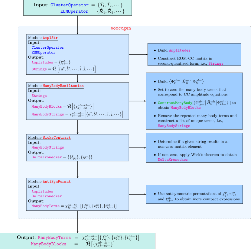
Figure 1: Flowchart of the entire set of modules constituting the EOM-CC equation generator.

III.1 Step 1

The first step is carried out through the module AmplStr. The inputs of this module are the ClusterOperator and EOMOperator:

$$\{{\color[rgb]{1,0,1}\texttt{Amplitudes}},{\color[rgb]{1,0,1}\texttt{Strings}}\}={\color[rgb]{1,0,0}\texttt{AmplStr}}\quantity[{\color[rgb]{0,0,1}\texttt{ClusterOperator}},{\color[rgb]{0,0,1}\texttt{EOMOperator}}]$$

It returns the list of CC amplitudes (stemming from the truncated Taylor expansion of $e^{\hat{T}}$) in Amplitudes. For example, in the case of EE-EOM-CCSD, we have

$${\color[rgb]{1,0,1}\texttt{Amplitudes}}=\{1,t_{{o}_{1}}^{{v}_{1}},t_{{o}_{1}}^{{v}_{1}}t_{{o}_{2}}^{{v}_{2}},t_{{o}_{1}}^{{v}_{1}}t_{{o}_{2}}^{{v}_{2}}t_{{o}_{3}}^{{v}_{3}},t_{{o}_{1}{o}_{2}}^{{v}_{1}{v}_{2}},t_{{o}_{1}{o}_{2}}^{{v}_{1}{v}_{2}}t_{{o}_{3}}^{{v}_{3}}\}$$

while, in mathematica, it takes the following form:

⬇

1 Amplitudes={{1},{t1$[\![$o1,v1$]\!]$},{t1$[\![$o1,v1$]\!]$t1$[\![$o2,v2$]\!]$},{t1$[\![$o1,v1$]\!]$t1$[\![$o2,v2$]\!]$t1$[\![$o3,v3$]\!]$},{t2$[\![$o1,o2,v1,v2$]\!]$},{t1$[\![$o1,v1$]\!]$t2$[\![$o2,o3,v2,v3$]\!]$}}

The set of excitation operators gathered in EOMOperator determines the basis in which $\boldsymbol{\mathcal{\bar{H}}}$ [see Eq. (29)] is diagonalized. With this basis together with the similarity-transformed Hamiltonian, the EOM-CC matrix is written in second-quantized form, $\boldsymbol{\mathcal{\bar{H}}}\quantity[\{\hat{p}^{{\dagger}}_{1},\hat{p}^{{\dagger}}_{2},\cdots,\hat{h}_{1},\hat{h}_{2},\cdots\}]$, and stored in the variable Strings, which is made of two substrings, i.e., ${\color[rgb]{1,0,1}\texttt{Strings}}=\{{\color[rgb]{1,0,1}\texttt{StringF}},{\color[rgb]{1,0,1}\texttt{StringV}}\}$, where StringF (F stands for $\hat{F}_{\text{N}}$) and StringV (V stands for $\hat{V}_{\text{N}}$). For example, the element ${\color[rgb]{1,0,1}\texttt{StringV}}[\![\texttt{2,1,6}]\!]$ corresponds to

$$\bra{D}\hat{V}_{\text{N}}\hat{T}_{1}\hat{T}_{2}\ket{S}=\\ \texttt{\{}\texttt{\{}\texttt{h1}^{{\dagger}}\texttt{,}\texttt{h2}^{{\dagger}}\texttt{,p2,p1\}}\texttt{,}\texttt{\{}\texttt{q1}^{{\dagger}}\texttt{,}\texttt{q2}^{{\dagger}}\texttt{,q4,q3\}}\texttt{,}\\ \texttt{\{}\texttt{\{}\texttt{v1}^{{\dagger}}\texttt{,}\texttt{o1\}{,}\{}\texttt{v2}^{{\dagger}}\texttt{,}\texttt{o2}\texttt{,}\texttt{v3}^{{\dagger}}\texttt{,}\texttt{o3\}\}}\texttt{,}\texttt{\{}\texttt{p3}^{{\dagger}}\texttt{,}\texttt{h3\}}\texttt{\}}$$

The values 2 and 1 in ${\color[rgb]{1,0,1}\texttt{StringV}}[\![\texttt{2,1,6}]\!]$ correspond to the indices of the row and column of the EOM-CC matrix, respectively, while 6 represents the sixth amplitude, i.e., ${\color[rgb]{1,0,1}\texttt{Amplitudes}}[\![\texttt{6}]\!]$. For the sake of simplicity, the summation and the Fermi vacuum of StringF and StringV are implicit.

III.2 Step 2

In Fig. 1, the module that corresponds to the second step is named ManyBodyHamiltonian and requires the input quantity Strings generated in AmplStr (see Subsec. III.1):

$$\{{\color[rgb]{1,0,1}\texttt{ManyBodyBlocks}},{\color[rgb]{1,0,1}\texttt{ManyBodyStrings}}\}={\color[rgb]{1,0,0}\texttt{ManyBodyHamiltonian}}\quantity[{\color[rgb]{1,0,1}\texttt{Strings}}]$$

where ManyBodyBlocks corresponds to the EOM-CC matrix defined in Eq. (29) written in terms of the many-body terms, i.e., $\boldsymbol{\mathcal{\bar{H}}}\quantity[\{\chi_{{h}_{1}{h}_{2}\cdots{p}_{3}{p}_{4}\cdots}^{{p}_{1}{p}_{2}\cdots{h}_{3}{h}_{4}\cdots}\}]$, and ManyBodyStrings is a list that consists of all unique many-body terms in second-quantized form, i.e., $\chi_{{h}_{1}{h}_{2}\cdots{p}_{3}{p}_{4}\cdots}^{{p}_{1}{p}_{2}\cdots{h}_{3}{h}_{4}\cdots}\quantity[\{\hat{p}^{{\dagger}}_{1},\hat{p}^{{\dagger}}_{2},\cdots,\hat{h}_{1},\hat{h}_{2},\cdots\}]$.

More precisely, the algorithm inside ManyBodyHamiltonian that generates ManyBodyBlocks and ManyBodyStrings performs the following steps:

1. Extract the EOM basis from Strings and evaluate the many-body Hamiltonian represented in Eq. (31) to form matrix elements, such as $\bra{\Phi_{{h}_{1}{h}_{2}\cdots}^{{p}_{1}{p}_{2}\cdots}}\bar{H}_{\text{N}}^{\text{mb}}\ket{\Phi_{{h}_{3}{h}_{4}\cdots}^{{p}_{3}{p}_{4}\cdots}}$.

2. Set to zero the many-body terms that correspond to the CC amplitude equations, such as the ones defined in Eq. (38).

3. Contract blocks made of second-quantized strings of the form $\bra{\Phi_{{h}_{1}{h}_{2}\cdots}^{{p}_{1}{p}_{2}\cdots}}\bar{H}_{\text{N}}^{\text{mb}}\ket{\Phi_{{h}_{3}{h}_{4}\cdots}^{{p}_{3}{p}_{4}\cdots}}$ with the help of the ContractManyBody function. For example, the contraction of the block $\bra{\Phi_{{h}_{1}}^{{p}_{1}}}\bar{H}_{\text{N}}^{\text{mb}}\ket{\Phi_{{h}_{3}}^{{p}_{3}}}$ generates

   $$(-\delta_{p_{1}p_{3}}\chi_{{h}_{1}}^{{h}_{3}},\delta_{h_{1}h_{3}}\chi_{{p}_{3}}^{{p}_{1}},-\chi_{{h}_{1}{p}_{3}}^{{p}_{1}{h}_{3}})={\color[rgb]{0,0.70703125,0}\texttt{ContractManyBody}}[\bra{\Phi_{{h}_{1}}^{{p}_{1}}}\bar{H}_{\text{N}}^{\text{mb}}\ket{\Phi_{{h}_{3}}^{{p}_{3}}}]$$

   Applying ContractManyBody to each block of $\boldsymbol{\mathcal{\bar{H}}}$ allows us to obtain the EOM-CC matrix in terms of many-body terms, i.e., $\boldsymbol{\mathcal{\bar{H}}}\quantity[\{\chi_{{h}_{1}{h}_{2}\cdots{p}_{3}{p}_{4}\cdots}^{{p}_{1}{p}_{2}\cdots{h}_{3}{h}_{4}\cdots}\}]$. These are stored in ManyBodyBlocks. In mathematica, it takes the following form:

   ⬇

   1 ManyBodyBlocks={-$\delta_{\texttt{p1,p3}}$$\chi$1$[\![$h3,h1$]\!]$+$\delta_{\texttt{h1,h3}}$$\chi$1$[\![$p1,p3$]\!]$-$\chi$2$[\![$h3,p1,h1,p3$]\!]$}

4. For each block of ManyBodyBlocks, we remove any redundant many-body term to create a list of unique terms, $\chi_{{h}_{1}{h}_{2}\cdots{p}_{3}{p}_{4}\cdots}^{{p}_{1}{p}_{2}\cdots{h}_{3}{h}_{4}\cdots}\quantity[\{\hat{p}^{{\dagger}}_{1},\hat{p}^{{\dagger}}_{2},\cdots,\hat{h}_{1},\hat{h}_{2},\cdots\}]$, stored in ManyBodyStrings. This is done by counting the number of hole-annihilation, hole-creation, particle-annihilation, and particle-creation operators in each term. For example, in the case of IP-EOM-CCSD, we have

   $${\color[rgb]{1,0,1}\texttt{ManyBodyStrings}}=\{\chi_{{h}_{1}}^{{h}_{3}},\chi_{{p}_{3}}^{{h}_{4}},\chi_{{p}_{3}}^{{p}_{1}},\chi_{{h}_{1}{h}_{2}}^{{h}_{3}{p}_{1}},\chi_{{h}_{2}{p}_{3}}^{{h}_{4}{p}_{1}},\chi_{{h}_{1}{h}_{2}{p}_{3}}^{{h}_{3}{h}_{4}{p}_{1}}\}$$

   Next, we express each many-body term as in Eq. (34) to obtain their second-quantized form. For example,

   $$\chi_{{h}_{1}{h}_{2}{p}_{3}}^{{h}_{3}{h}_{4}{p}_{1}}=\bra{\Phi_{{h}_{1}{h}_{2}}^{{p}_{1}}}\bar{H}_{\text{N}}^{\text{st}}\ket{\Phi_{{h}_{3}{h}_{4}}^{{p}_{3}}}_{iC}$$ (40)

   while, in mathematica, this three-body term corresponds to the sixth position of ManyBodyStrings:

   ⬇

   1 ManyBodyBlocks$[\![$6$]\!]$={{{SuperDagger[h1],SuperDagger[h2],p1},{SuperDagger[q1],SuperDagger[q2],q4,q3},{},{SuperDagger[p3],h4,h3}},{{SuperDagger[h1],SuperDagger[h2],p1},{SuperDagger[q1],SuperDagger[q2],q4,q3},{{SuperDagger[v1],o1}},{SuperDagger[p3],h4,h3}},{{SuperDagger[h1],SuperDagger[h2],p1},{SuperDagger[q1],SuperDagger[q2],q4,q3},{{SuperDagger[v1],o1},{SuperDagger[v2],o2}},{SuperDagger[p3],h4,h3}},{{SuperDagger[h1],SuperDagger[h2],p1},{SuperDagger[q1],SuperDagger[q2],q4,q3},{{SuperDagger[v1],o1},{SuperDagger[v2],o2},{SuperDagger[v3],o3}},{SuperDagger[p3],h4,h3}},{{SuperDagger[h1],SuperDagger[h2],p1},{SuperDagger[q1],SuperDagger[q2],q4,q3},{{SuperDagger[v1],o1,SuperDagger[v2],o2}},{SuperDagger[p3],h4,h3}},{{SuperDagger[h1],SuperDagger[h2],p1},{SuperDagger[q1],SuperDagger[q2],q4,q3},{{SuperDagger[v1],o1},{SuperDagger[v2],o2,SuperDagger[v3],o3}},{SuperDagger[p3],h4,h3}}}\end{lstlisting}

   2

   3\end{enumerate}

   4

   5%=====================%

   6\subsection{Step 3}

   7\label{subsec:stp3}

   8%=====================%

   9The third step is carried out by the module named \red{\texttt{WicksContract}}, which performs Wick’s contractions [see Eq.~\eqref{eq:wickno}] of the second-quantized strings in \brown{\texttt{ManyBodyStrings}} obtained in the module \red{\texttt{ManyBodyHamiltonian}}, as follows:

   10\begin{equation*}

   11 \brown{\texttt{DeltaKronecker}}=

   12 \\

   13 \red{\texttt{WicksContract}}[\brown{\texttt{ManyBodyStrings}} ]

   14\end{equation*}

   15The output \brown{\texttt{DeltaKronecker}} contains two quantities, the Kronecker deltas and the signs of each contraction.

   16

   17Figure \ref{Fig:wickscontract} illustrates the structure of the module \red{\texttt{WicksContract}}.

   18Its input is the one-body term $\chi_{{p}_{1}}^{{h}_{1}}$ which is stored in the variable ${\color[rgb]{1,0,1}\texttt{ManyBodyStrings}}[\![\texttt{3}]\!]$ produced by the module \red{\texttt{ManyBodyHamiltonian}} discussed in Subsec.~\ref{subsec:stp2}.

   19The first step consists of replacing the similarity-transformed Hamiltonian with the terms yielding non-zero matrix elements and then applying Wick’s theorem to the remaining terms.

   20Finally, the Kronecker deltas and signs obtained from Wick’s theorem are stored in \brown{\texttt{DeltaKronecker}}.

   21

   22%%% FIG 2 %%%

   23\begin{figure*}

   24 \includegraphics[width=0.6\textwidth]{figure2}

   25 \caption{Flowchart of the module \red{\texttt{WicksContract}}.

   26 The module takes as input $\chi_{{p}_{1}}^{{h}_{1}}=\matrixelement{0}{\bar{H}_{\text{N}}}{\Phi_{{h}_{1}}^{{p}_{1}}}_{iC}$ stored in the variable \brown{\texttt{ManyBodyStrings}} produced from the module \red{\texttt{ManyBodyHamiltonian}} (see Fig.~\ref{Fig:eomccalg}).}

   27 \label{Fig:wickscontract}

   28\end{figure*}

   29

   30%=====================%

   31\subsection{Step 4}

   32\label{subsec:stp4}

   33%=====================%

   34

   35The module \red{\texttt{AntiSymPermut}} requires three inputs: \brown{\texttt{DeltaKronecker}}, \brown{\texttt{ManyBodyStrings}}, and \brown{\texttt{Amplitudes}}.

   36\begin{equation*}

   37 \brown{\texttt{ManyBodyTerms}}=

   38 \red{\texttt{AntiSymPermut}}[\brown{\texttt{DeltaKronecker}},\brown{\texttt{ManyBodyStrings}},\brown{\texttt{Amplitudes}} ]

   39\end{equation*}

   40This module applies the Kronecker deltas obtained in \red{\texttt{WicksContract}} (see Subsec.~\ref{subsec:stp3}) to the \brown{\texttt{Amplitudes}} (generated in \red{\texttt{AmplStr}} and discussed in Subsec.~\ref{subsec:stp1}), the Fock matrix elements, $\{f_{q}^{p}\}$, and the two-electron repulsion integrals, $\{v_{rs}^{pq}\}$.

   41Next, it takes advantage of the antisymmetric permutations of the amplitudes and integrals to obtain more compact expressions.

   42

   43Finally, as output, \brown{\texttt{ManyBodyBlocks}} obtained in the module \red{\texttt{ManyBodyHamiltonian}} (see Subsec.~\ref{subsec:stp2}) and \brown{\texttt{ManyBodyTerms}}, $\chi_{{h}_{1}{h}_{2}\cdots{p}_{3}{p}_{4}\cdots}^{{p}_{1}{p}_{2}\cdots{h}_{3}{h}_{4}\cdots}\quantity[\{f_{q}^{p}\},\{v_{rs}^{pq}\},\{t_{{h}_{1}{h}_{2}\cdots}^{{p}_{1}{p}_{2}\cdots}\}]$, from \red{\texttt{AntiSymPermut}} are printed.

   44From these, one can easily generate the EOM-CC equations.

   45

   46%=====================%

   47\subsection{Examples}

   48\label{subsec:examples}

   49%=====================%

   50

   51The software has also the advantage of being able to generate various outputs, including CC energy and amplitude equations, second-quantized strings in normal order, many-body terms of the similarity-transformed Hamiltonian, and blocks of the EOM-CC Hamiltonian matrix in terms of many-body terms.

   52

   53For example, the input code to obtain IP-EOM-CCSD is

   54\begin{lstlisting}[language=Mathematica]

   55 (* Input for IP-EOM-CCSD *)

   56

   57 ClusterOperator={{"1h1p"},{"2h2p"}};

   58 EOMOperator={{"1h0p"},{"2h1p"}};

   59 eomccgen[ClusterOperator,EOMOperator]

   while the output consists of a list of many-body terms and the EOM-CC matrix in terms of these quantities:

   ⬇

   1 (* Many-body terms *)

   2

   3 $\chi$1$[\![$h3,h1$]\!]$==-F$[\![$h3,h1$]\!]$-F$[\![$h3,v1$]\!]$t1$[\![$h1,v1$]\!]$+t1$[\![$o1,v1$]\!]$ERI$[\![$h3,o1,v1,h1$]\!]$+

   4 t1$[\![$h1,v2$]\!]$t1$[\![$o1,v1$]\!]$ERI$[\![$h3,o1,v1,v2$]\!]$+1/2t2$[\![$o1,h1,v1,v2$]\!]$ERI$[\![$h3,o1,v1,v2$]\!]$

   5 $\chi$1$[\![$h4,p3$]\!]$==F$[\![$h4,p3$]\!]$-t1$[\![$o1,v1$]\!]$ERI$[\![$h4,o1,v1,p3$]\!]$

   6 $\chi$2$[\![$h4,h3,h1,p3$]\!]$==ERI$[\![$h4,h3,h1,p3$]\!]$+t1$[\![$h1,v1$]\!]$ERI$[\![$h4,h3,v1,p3$]\!]$

   7 $\chi$2$[\![$h3,p1,h1,h2$]\!]$==t1$[\![$o1,p1$]\!]$ERI$[\![$h3,o1,h1,h2$]\!]$-t1$[\![$h2,v1$]\!]$t1$[\![$o1,p1$]\!]$ERI$[\![$h3,o1,v1,h1$]\!]$+

   8 t1$[\![$h1,v1$]\!]$t1$[\![$o1,p1$]\!]$ERI$[\![$h3,o1,v1,h2$]\!]$+t1$[\![$h1,v1$]\!]$t1$[\![$h2,v2$]\!]$t1$[\![$o1,p1$]\!]$ERI$[\![$h3,o1,v1,v2$]\!]$-

   9 ERI$[\![$h3,p1,h1,h2$]\!]$+t1$[\![$h2,v1$]\!]$ ERI$[\![$h3,p1,v1,h1$]\!]$-t1$[\![$h1,v1$]\!]$ ERI$[\![$h3,p1,v1,h2$]\!]$-

   10 t1$[\![$h1,v1$]\!]$t1$[\![$h2,v2$]\!]$ERI$[\![$h3,p1,v1,v2$]\!]$-F$[\![$h3,v1$]\!]$t2$[\![$h1,h2,v1,p1$]\!]$+

   11 1/2t1$[\![$o1,p1$]\!]$t2$[\![$h1,h2,v1,v2$]\!]$ERI$[\![$h3,o1,v1,v2$]\!]$-1/2ERI$[\![$h3,p1,v1,v2$]\!]$t2$[\![$h1,h2,v1,v2$]\!]$+

   12 t1$[\![$o1,v1$]\!]$t2$[\![$h1,h2,v2,p1$]\!]$ERI$[\![$h3,o1,v1,v2$]\!]$-t2$[\![$o1,h1,v1,p1$]\!]$ERI$[\![$h3,o1,v1,h2$]\!]$

   13 +t1$[\![$h2,v1$]\!]$t2$[\![$o1,h1,v2,p1$]\!]$ERI$[\![$h3,o1,v1,v2$]\!]$+t2$[\![$o1,h2,v1,p1$]\!]$ERI$[\![$h3,o1,v1,h1$]\!]$

   14 -t1$[\![$h1,v1$]\!]$t2$[\![$o1,h2,v2,p1$]\!]$ ERI$[\![$h3,o1,v1,v2$]\!]$

   15 $\chi$1$[\![$p1,p3$]\!]$==F$[\![$p1,p3$]\!]$-F$[\![$o1,p3$]\!]$ t1$[\![$o1,p1$]\!]$-t1$[\![$o1,v1$]\!]$ t1$[\![$o2,p1$]\!]$ ERI$[\![$o1,o2,v1,p3$]\!]$+t1$[\![$o1,v1$]\!]$ ERI$[\![$o1,p1,v1,p3$]\!]$-1/2ERI$[\![$o1,o2,v1,p3$]\!]$t2$[\![$o1,o2,v1,p1$]\!]$

   16 $\chi$2$[\![$h4,h3,h1,h2$]\!]$==-ERI$[\![$h4,h3,h1,h2$]\!]$+t1$[\![$h2,v1$]\!]$ ERI$[\![$h4,h3,v1,h1$]\!]$-t1$[\![$h1,v1$]\!]$ ERI$[\![$h4,h3,v1,h2$]\!]$-t1$[\![$h1,v1$]\!]$ t1$[\![$h2,v2$]\!]$ ERI$[\![$h4,h3,v1,v2$]\!]$-1/2 ERI$[\![$h4,h3,v1,v2$]\!]$ t2$[\![$h1,h2,v1,v2$]\!]$

   17 $\chi$2$[\![$h4,p1,h2,p3$]\!]$==t1$[\![$o1,p1$]\!]$ ERI$[\![$h4,o1,h2,p3$]\!]$+t1$[\![$h2,v1$]\!]$t1$[\![$o1,p1$]\!]$ERI$[\![$h4,o1,v1,p3$]\!]$-ERI$[\![$h4,p1,h2,p3$]\!]$

   18 -t1$[\![$h2,v1$]\!]$ ERI$[\![$h4,p1,v1,p3$]\!]$-ERI$[\![$h4,o1,v1,p3$]\!]$ t2$[\![$o1,h2,v1,p1$]\!]$

   19 $\chi$3$[\![$h4,h3,p1,h1,h2,p3$]\!]$==ERI$[\![$h4,h3,v1,p3$]\!]$ t2$[\![$h1,h2,v1,p1$]\!]$

   20

   21 (* EOM-CC blocks *)

   22

   23 {{-$\chi$1$[\![$h3,h1$]\!]$},

   24 {$\chi$2$[\![$h4,h3, h1, p3$]\!]$+$\delta_{\texttt{h1,h3}}$$\chi$1$[\![$h4,p3$]\!]$-$\delta_{\texttt{h1,h4}}$$\chi$1$[\![$h3,p3$]\!]$},

   25 {-$\chi$2$[\![$h3,p1,h2,h1$]\!]$},

   26 {-$\chi$1$[\![$h4,h2$]\!]$$\delta_{\texttt{h1,h3}}$$\delta_{\texttt{p1,p3}}$+$\chi$1$[\![$h3,h2$]\!]$$\delta_{\texttt{h1,h4}}$$\delta_{\texttt{p1,p3}}$+$\chi$1$[\![$h4,h1$]\!]$$\delta_{\texttt{h2,h3}}$$\delta_{\texttt{p1,p3}}$-$\chi$1$[\![$h3,h1$]\!]$$\delta_{\texttt{h2,h4}}$$\delta_{\texttt{p1,p3}}$-$\chi$1$[\![$p1,p3$]\!]$$\delta_{\texttt{h1,h4}}$$\delta_{\texttt{h2,h3}}$

   27 +$\chi$1$[\![$p1,p3$]\!]$$\delta_{\texttt{h1,h3}}$$\delta_{\texttt{h2,h4}}$-$\chi$2$[\![$h4,p1,h2,p3$]\!]$$\delta_{\texttt{h1,h3}}$+$\chi$2$[\![$h3,p1,h2,p3$]\!]$$\delta_{\texttt{h1,h4}}$+$\chi$2$[\![$h4,p1, h1,p3$]\!]$$\delta_{\texttt{h2,h3}}$- $\chi$2$[\![$h3,p1,h1,p3$]\!]$$\delta_{\texttt{h2,h4}}$+

   28 $\chi$2$[\![$h4,h3,h2,h1$]\!]$$\delta_{\texttt{p1,p3}}$+$\chi$3$[\![$h4,h3,p1,h2,h1,p3$]\!]$}}

   The input code to generate the CCD equations is

   ⬇

   1 (* Input for CCD *)

   2

   3 ClusterOperator={{"2h2p"}};

   4 EOMOperator={{"0h0p"}};

   5 eomccgen[ClusterOperator,EOMOperator]

   and it produces the following output:

   ⬇

   1 (* CCD energy *)

   2

   3 {1/4 ERI$[\![$o1,o2,v1,v2$]\!]$ t2$[\![$o1,o2,v1,v2$]\!]$}

   4

   5 (* T2 equations *)

   6

   7 {-ERI$[\![$p2,p1,h1,h2$]\!]$

   8 -F$[\![$p2,v1$]\!]$t2$[\![$h1,h2,v1,p1$]\!]$+F$[\![$p1,v1$]\!]$t2$[\![$h1,h2,v1,p2$]\!]$

   9 -F$[\![$o1,h2$]\!]$t2$[\![$o1,h1,p2,p1$]\!]$+F$[\![$o1,h1$]\!]$t2$[\![$o1,h2,p2,p1$]\!]$

   10 -1/2 ERI$[\![$p2,p1,v1,v2$]\!]$t2$[\![$h1,h2,v1,v2$]\!]$ +ERI$[\![$o1,p2,v1,h2$]\!]$t2$[\![$o1,h1,v1,p1$]\!]$

   11 -ERI$[\![$o1,p1,v1,h2$]\!]$t2$[\![$o1,h1,v1,p2$]\!]$-ERI$[\![$o1,p2,v1,h1$]\!]$t2$[\![$o1,h2,v1,p1$]\!]$

   12 +ERI$[\![$o1,p1,v1,h1$]\!]$t2$[\![$o1,h2,v1,p2$]\!]$-1/2ERI$[\![$o1,o2,h1,h2$]\!]$t2$[\![$o1,o2,p2,p1$]\!]$

   13 -1/4ERI$[\![$o1,o2,v1,v2$]\!]$t2$[\![$h1,h2,v1,v2$]\!]$t2$[\![$o1,o2,p2,p1$]\!]$

   14 -1/2ERI$[\![$$[\![$o1,o2,v1,v2$]\!]$t2$[\![$h1,h2,v2,p2$]\!]$t2$[\![$o1,o2,v1,p1$]\!]$

   15 +1/2ERI$[\![$o1,o2,v1,v2$]\!]$t2$[\![$h1,h2,v2,p1$]\!]$t2$[\![$o1,o2,v1,p2$]\!]$

   16 -1/2ERI$[\![$o1,o2,v1,v2$]\!]$t2$[\![$o1,h2,v1,v2$]\!]$t2$[\![$o2,h1,p2,p1$]\!]$

   17 +1/2ERI$[\![$o1,o2,v1,v2$]\!]$t2$[\![$o1,h1,v1,v2$]\!]$t2$[\![$o2,h2,p2,p1$]\!]$

   18 +ERI$[\![$o1,o2,v1,v2$]\!]$t2$[\![$o1,h2,v1,p2$]\!]$t2$[\![$o2,h1,v2,p1$]\!]$

   19 -ERI$[\![$o1,o2,v1,v2$]\!]$t2$[\![$o1,h1,v1,p2$]\!]$t2$[\![$o2,h2,v2,p1$]\!]$}

   In the following example, we compute the block {2,1} of the IP-EOM-CCSD matrix. The corresponding input is

   ⬇

   1 (* Input for IP-EOM-CCSD *)

   2

   3 ClusterOperator={{"1h0p"},{"2h1p"}};

   4 EOMOperator={{"1h1p"},{"2h2p"}};

   5 EOMBlock={2,1};

   6 eomccgen[ClusterOperator,EOMOperator,EOMBlock]

   and the output is

   ⬇

   1 (* Many body terms *)

   2

   3 $\chi$1$[\![$h4,p3$]\!]$==F$[\![$h4,p3$]\!]$-ERI$[\![$h4,o1,v1,p3$]\!]$t1$[\![$o1,v1$]\!]$

   4 $\chi$2$[\![$h4,h3,h1,p3$]\!]$==ERI$[\![$h4,h3,h1,p3$]\!]$-ERI$[\![$h4,h3,v1,p3$]\!]$t1$[\![$h1,v1$]\!]$

   5

   6 (* EOM-CC blocks *)

   7

   8 {$\chi$1$[\![$h4,p3$]\!]$$\delta_{\texttt{h1,h3}}$-$\chi$1$[\![$h3,p3$]\!]$$\delta_{\texttt{h1,h4}}$+$\chi$2$[\![$h4,h3,v1,p3$]\!]$}

   It is also possible to contract the EOM-CC Hamiltonian and the right or left eigenvectors [see Eqs. (29) and (30)]. These quantities are useful when one relies on the Davidson diagonalization method [79] or related techniques. For example, the input to obtain the left-hand eigenvalue equation for IP-EOM-CCSD is the following:

   ⬇

   1 (* Input for IP-EOM-CCSD *)

   2

   3 ClusterOperator={{"1h0p"},{"2h1p"}};

   4 EOMOperator={{"1h1p"},{"2h2p"}};

   5 LeftRigthEOM={"L"};

   6 eomccgen[ClusterOperator,EOMOperator,LeftRigthEOM]

   The output is very similar to the first example with the difference that, in ManyBodyBlocks, the Kronecker deltas are applied to the many-body terms as well as to the left-hand EOM-CC amplitudes.

   The mathematica code described in this paper is publicly available in a dedicated repository on github with the name eomccgen. [80] In particular, the repository contains examples of scripts and data files that can be easily adapted for particular research projects. Additionally, the repository includes another notebook, called eomccnum, where the equations obtained in eomccgen can be implemented and numerically tested for small atoms and molecules. eomccnum comes with pre-installed examples that can serve as a guide for implementing the equations obtained in eomccgen. An example of the water molecule in the STO-3G basis can be found in the repository.

   IV Conclusion

   The present paper discusses the development of a code generator for equation-of-motion coupled-cluster (EOM-CC) methods, a class of many-body quantum chemistry methods known for their accuracy in predicting excitation energies, ionization potentials, and electron affinities in molecular systems. Because their implementation can be complex and time-consuming, we develop an easy-to-use code generator that automates the process of deriving and implementing the EOM-CC equations, reducing the potential for human error.

   We begin by discussing the second-quantization formalism, a practical and modern mathematical language used to describe many-body quantum systems in terms of creation and annihilation operators. We then discuss the development of our code generator for EOM-CC methods. Our approach builds on previous work by using second-quantized strings to automate the derivation and implementation of EOM-CC equations. However, we introduce several new features that make the code generator more efficient and flexible. For example, we rely on a symbolic algebra software package, mathematica, to generate these equations that can be easily read by humans and machines. The paper provides a detailed description of each step of the algorithm used in the code generator. We also describe how the code generator can be used to calculate excitation energies, ionization potentials, and electron affinities, by providing several concrete examples.

   Although many improvements are still needed to generate a production-level code, especially in the definition of adequate intermediates to ensure the right computational scaling of the methods, we hope that the present work illustrates nicely the capabilities of mathematica-based code generator in the context of CC theory.