Abstract

A survey is given on the current status of the theoretical description of unpolarized and polarized deep–inelastic scattering processes in Quantum Chromodynamics at large virtualities.

Chapter 0 Deep-Inelastic Scattering: What do we know ?

Dedicated to the Memory of Harald Fritzsch.

1 Introduction

About 50 years ago Quantum Chromodynamics (QCD), the theory of strong interactions, was found [1, 2, 3, 4, 5], and Harald Fritzsch played a major role in this. After the proof of renormalizibility [6, 7] of the Yang-Mills theories [8] and the proof of the anomaly freedom [9] of the $SU_{2L}\times U_{1Y}\times SU_{3c}$ Standard Model, systematic perturbative calculations became possible to make predictions for experimental precision measurements of several hard scattering processes under certain kinematic conditions. The first calculation concerned the running of the strong coupling constant [3, 4] proving asymptotic freedom, a conditio sine qua non for higher order calculations in perturbative QCD. One of the key processes is deeply inelastic scattering (DIS) of leptons off nucleons, both in the unpolarized and polarized case. These processes allow to determine the various quark flavor and gluon densities [10, 11, 12, 13], reveal higher twist contributions in the region of low virtualities $Q^{2}$ and/or large values of the Bjorken variable $x$,[14, 15], with $x=Q^{2}/(2p.q)$, $Q^{2}=-q^{2}$, $q$ the 4-momentum transfer from the lepton to the nucleon, and $p$ the nucleon momentum.

Deep–inelastic scattering has been the method to observe scaling [16], predicted in Ref. [17] and leading to the parton model [18]. It allows to measure the strong coupling constant $\alpha_{s}(M_{Z}^{2})$ at high precision [19] from the scaling violations of the deep–inelastic structure functions [20]. Furthermore, their heavy flavor contributions allow a precision measurement of the charm quark mass $m_{c}$ [21].

In this survey we will sketch the way the QCD corrections to deep–inelastic scattering took from the beginning of the light-cone picture [22] and (naive) parton model [18] until today, concerning the running of the coupling, the anomalous dimensions, the different massless and massive Wilson coefficients in both the unpolarized and polarized case. The corrections to the QCD $\beta$–function, being a zero–scale quantity, are simpler to calculate than the anomalous dimensions for general values of the Mellin variable $N$, which are somewhat simpler than the massless Wilson coefficients, followed in complexity by analytic results on the massive Wilson coefficients.

For the unpolarized anomalous dimensions the first order corrections were known in 1974, the second order corrections in 1980 (with a final correction in 1991), and the third order results in 2004. The main massless Wilson coefficients were known in correct form 1980 at one loop, in 1992 at two loops and 2005 at three loops. In the massive case the one loop results were known in 1976, the two-loop results emerged between 1992 and 1996, and the asymptotic three loop results between 2010 and today, in the single and two–mass cases. The first fixed Mellin moments of these quantities were available earlier, if they had been calculated, and a series of lower moments has been calculated at four–loop order since 2016. The QCD $\beta$ function is known to five–loop order since 2016/17. This time–line shows the challenge, which in part had to involve new mathematical developments and certainly great efforts in computer algebra.

We will describe this development for the anomalous dimensions, the Wilson coefficients and the renormalization-group quantities in the following, which form the asset needed to describe the scaling violations of the deep–inelastic structure functions. Furthermore, we will add some remarks on the Drell–Yan process, since these data are needed to fix the light sea–quark distributions in QCD analyzes. We will also comment on technical and mathematical challenges connected to these analytic calculations, which became indispensable since the time of about 1998 and were essential to achieve the present status.

2 Scaling violations of DIS structure functions

The measurement of the fundamental parameters of the Standard Model, such as $\alpha_{s}(M_{Z}^{2})$ or the heavy quark masses $m_{Q}$, require clear conditions. One has to choose a kinematic region for which definite theoretical predictions can be made. Here one request is that non–perturbative and perturbative effects can be clearly separated and the perturbative corrections can be carried out safely. In deep–inelastic scattering one is therefore advised to consider the kinematic region of the dominance of twist[26] $\tau=2$ operators, which means that the virtuality $Q^{2}$ of the process must be large to approach the Bjorken limit [17]. The effect of the higher twist contributions [14, 15] is then suppressed. One might choose to include only data with $Q^{2}>25$ GeV² and $W^{2}=Q^{2}(1-x)/x>12.5$ GeV² into the analysis, despite the fact of a high statistics measured below these scales, to avoid biases of not completely known power- and other corrections. It is known, cf. Ref. [15], that one may obtain different Standard Model parameters if these cuts are weakened pointing to corrections not being controlled.

Moreover, one may use the asymptotic heavy quark Wilson coefficients in this region [27], which can be calculated analytically, cf. Section 6. Under these conditions one obtains the single particle factorization [28] between the process-dependent Wilson coefficients and the single parton distribution functions, which is otherwise not the case. In going systematically to higher and higher orders there are also no limitations in approaching the small $x$ region, since the calculation within QCD is complete. Small $x$ approaches have to rely on factorization between the perturbative and non–perturbative contributions [28] as well and refer to the twist expansion for consistent renormalization. As has been shown in [29, 30], several sub–leading small $x$ series have to be known to obtain results which are phenomenologically stable. In the following we will concentrate on the theoretical calculations under the above conditions.

Let us consider the dynamics in Mellin $N$ space. The Mellin transform of a function $f(x)$ is given by

$$f(N)=\int_{0}^{1}dxx^{N-1}~{}\hat{f}(x).$$ (1)

In the twist–2 approximation the deep–inelastic structure functions $F_{i}$ obey the representation

$$F_{i}(N,Q^{2})=\sum_{l=q,g}C_{i,l}(N,a_{s},Q^{2}/\mu^{2})\cdot f_{l}(N,a_{s}),$$ (2)

where $C_{i,l}(N,Q^{2}/\mu^{2})$ denote the renormalized Wilson coefficients, $f_{l}$ the renormalized parton distribution functions, and $a_{s}=\alpha_{s}/(4\pi)$. Introducing the operator[31]

$${\mathscr{D}}(\mu^{2}):=\mu^{2}\frac{\partial}{\partial\mu^{2}}+\beta(a_{s}(\mu^{2}))\frac{\partial}{\partial a_{s}(\mu^{2})}-\gamma_{m}(a_{s}(\mu^{2}))m(\mu^{2})\frac{\partial}{\partial m(\mu^{2})},$$ (3)

with

$$\beta(a_{s}(\mu^{2})) = \mu^{2}\frac{\partial a_{s}(\mu^{2})}{\partial\mu^{2}},~{}~{}~{}\gamma_{m}(a_{s}(\mu^{2}))=-\frac{\mu^{2}}{m(\mu^{2})}\frac{\partial m(\mu^{2})}{\partial\mu^{2}}~{},$$ (4)

one obtains the following renormalization group equations (RGEs) from (2)

$$\sum_{j}\left[{\cal D}(\mu^{2})\delta_{ij}+\gamma_{ij}^{\rm S,NS}-n_{\psi}\gamma_{\psi}-n_{A}\gamma_{A}\right]f_{j}(N,\mu^{2}) = 0,$$ (5)

$$\sum_{j}\left[{\cal D}(\mu^{2})\delta_{ij}+\gamma_{J_{1}}+\gamma_{J_{2}}-\gamma_{ij}^{\rm S,NS}\right]C_{i}\left(N,\frac{Q^{2}}{\mu^{2}}\right) = 0~{}.$$ (6)

Here $\gamma_{\psi}$, $\gamma_{A}$ and $\gamma_{J_{1,2}}$ denote the anomalous dimension of external quarks, gluons, and the currents, which can be non-zero if the currents are not conserved. $\gamma_{ij}^{\rm S,NS}$ denote the anomalous dimensions of the local operators (16, 17). The scale dependence is due to $a_{s}(\mu^{2})$,

$$\mu^{2}\frac{da_{s}(\mu^{2})}{d\mu^{2}}=-\sum_{k=0}^{\infty}\beta_{k}a_{s}^{k+2}(\mu^{2}),$$ (7)

where one finally considers $\mu^{2}=Q^{2}$.

3 Zero scale quantities

The renormalization group equations for the massless and massive operator matrix elements and the Wilson coefficients also describe the scale dependence of the strong coupling constant and of the heavy quark masses. These are zero scale quantities and they have to be calculated to the respective order in perturbation theory. The running of the coupling constant $\alpha_{s}(\mu^{2})$ is described by (7). Similar equations hold for the other quantities. In the $\overline{\rm MS}$ scheme one may compute the different $Z$-factors renormalizing QCD in the case that there are no composite operators.

The one–loop result for the QCD $\beta$–function has been calculated in Refs. [3, 4], the two–loop corrections in Refs. [32], the three–loop contributions in Refs. [33], the four–loop corrections in Refs. [34], and most recently the five–loop corrections in Refs. [35]. The effect of asymptotic freedom observed in [3, 4] is refined by the higher order corrections for the number of active quark flavors $N_{F}\leq 6$ of nature. The other $Z$–factors to renormalize QCD were calculated in higher orders in Refs. [36, 37, 38, 39, 40] and are now also available at five–loop order. The running of the heavy quark masses and the wave function renormalization have been calculated in Refs. [41]. Herewith all necessary $Z$-factors occurring in processes without local operators are known.

4 Anomalous dimensions and splitting functions

The QCD evolution of the twist–2 parton densities is ruled by the anomalous dimensions in $N$ space, $\gamma_{ij}(N)$, or the splitting functions in $x$ space, where the latter are the inverse Mellin transform of the former. The evolution equations derive from the RGE (5) in non–singlet and singlet cases,

$$\frac{df_{i}^{\rm NS}(N,\mu^{2})}{d\ln(\mu^{2})}~{} = ~{}-\gamma_{qq}^{\rm NS}(N,a_{s})f_{i}^{\rm NS}(N,\mu^{2}),$$ (8)

$$\frac{d}{d\ln(\mu^{2})}\Biggl{[}\begin{array}[]{c}\Sigma(N,\mu^{2})\\ G(N,\mu^{2})\end{array}\Biggr{]}~{} = ~{}-\Biggl{[}\begin{array}[]{cc}\gamma_{qq}(N,a_{s})&\gamma_{qg}(N,a_{s})\\ \gamma_{gq}(N,a_{s})&\gamma_{gg}(N,a_{s})\end{array}\Biggr{]}\Biggl{[}\begin{array}[]{c}\Sigma(N,\mu^{2})\\ G(N,\mu^{2})\end{array}\Biggr{]},$$ (15)

with $i=1,2,3$ and $a_{s}=a_{s}(\mu^{2})$. The twist-2 parton densities are given as forward matrix elements $\langle i|O_{k}|j\rangle$ of the composite operators

$$O^{\sf NS}_{q;r;\mu_{1},\ldots,\mu_{n}}(0) = i^{N-1}{\bf S}\left[\bar{\psi}\gamma_{\mu_{1}}D_{\mu_{2}}\ldots D_{\mu_{N}}\frac{\lambda_{r}}{2}\psi\right],$$ (16)

$$O^{\sf S}_{q;r;\mu_{1},\ldots,\mu_{n}}(0) = i^{N-1}{\bf S}\left[\bar{\psi}\gamma_{\mu_{1}}D_{\mu_{2}}\ldots D_{\mu_{N}}\psi\right],$$ (17)

$$O^{\sf S}_{g;r;\mu_{1},\ldots,\mu_{n}}(0) = 2i^{N-2}{\bf S}{\bf Sp}\left[F^{a}_{\beta\gamma}D_{\mu_{2}}\ldots D_{\mu_{N-1}}F^{\alpha,a}_{\mu_{N}}\right],$$ (18)

in the unpolarized case (with similar expressions in the polarized case). Here the indices $q$ and $g$ refer to quark and gluon field operators, respectively, and $\lambda_{r}$ denotes the Gell-Mann matrix of the corresponding light flavor representation; $\psi$ is the quark field, $D_{\mu}$ the covariant derivative, $F^{a}_{\alpha\beta}$ the Yang–Mills field strength tensor, S the symmetry operator for all Lorentz indices and Sp the color-trace, where the index $a$ is the color index in the adjoint representation. One calculates both the fixed Mellin moments using certain techniques as well as the complete functions for general values of $N$. Here either the even or odd values of $N$ contribute, depending on the respective amplitude crossing relations, cf. [23, 42].

1 Fixed Moments

The first information one obtains on the anomalous dimensions is given by their fixed moments. One may calculate them by differentiating the forward Compton amplitude by the proton momentum $p$. In this way one works without reference, however, equivalent to the local twist two operators. The method has the advantage that also the moments of the respective massless Wilson coefficients can be obtained in this way. In the massless case the Mincer algorithm has been used [43] to three–loop order. In the massive case one uses the package MATAD [44]. At two–loop order this has been done in Ref. [45]. The method has later been expanded to three–loop order in Refs. [46], reaching an intermediate technical limit calculating the 16th moment in the flavor non–singlet case in 2003. In the case of massive operator matrix elements (OMEs) moments between $N=10$ and $N=16$ were calculated in Ref. [47] at three–loop order. In the two–mass case moments were calculated in Refs. [48]. The method implies an exponential rise of terms to be calculated and therefore terminates at a given order, depending on the complexity of the given problem.

More recently, also a series of lower moments at four– and five–loop order have been calculated by basically the same method in Refs. [49, 50], using Forcer [51] now having reached $N=20$ in the four–loop case. This provides the most far reaching information at the moment. For simpler structures the number of moments obtained allow the reconstruction of the general $N$ results under certain assumptions [49], in particular also that only harmonic sums [52] contribute.

As known from the light–cone expansion [22], the Mellin moments are the genuine quantities in describing the scaling violations of DIS structure functions. In any approach to the calculation of DIS anomalous dimensions and Wilson coefficients one may transform the integration-by-parts identities (IBP) [53] into difference equations for the master integrals, and related to that, the amplitude. By using the method of arbitrarily high moments [54] one may calculate very effectively high numbers of moments. Even in the massive case we have generated 15.000 moments at three–loop order recently.

The method of Ref. [54] allows then to use the method of guessing [55] to find the associated recurrence, given one has had a sufficient number of moments. Here no special assumptions on the mathematical structure of the results are made unlike in the approach used e.g. in Ref. [49]. The obtained recurrences are then inspected using difference ring theory algorithms as implemented in the package Sigma [56]. In the case of first order factorizing problems the general $N$ solution can be calculated. In all other cases the first order factors can be separated off. This method could be applied to all anomalous dimensions and massless Wilson coefficients to three loop order, which are first–order factorizable problems. This also applies to various massive Wilson coefficients at three–loop order, as will be discussed below.

The calculation of the Mellin moments by using the differentiation method is very different form other approaches. Therefore these results provide firm checks on the results for the case of general $N$ recurrences, without making special assumptions.

2 Results at General $N$

The leading order unpolarized anomalous dimensions were calculated in Refs. [20] and in the polarized case in [57]. A partonic approach has been used in Ref. [58], which is related to Refs. [20, 57] by a Mellin transform. The next-to-leading order anomalous dimensions and splitting functions were computed in Refs. [59, 60] resp. in Refs. [61]. Finally, the next-to-next-to-leading order ones in Refs. [62, 63, 64, 65, 66, 67, 68, 69, 70] and Refs. [71, 72, 73, 65] in the unpolarized and polarized cases. Simpler color factors at four–loops are available at general values of $N$ [50, 74]. Here different techniques have been used, such as the forward Compton amplitude [62, 63, 71, 65], massive on–shell OMEs [66, 67, 72] massless off–shell OMEs [64, 73, 70], and different hard scattering cross sections with on–shell amplitudes [68, 69]. All contributions can be expressed in terms of harmonic sums or in $x$–space by the corresponding Mellin inversion in terms of harmonic polylogarithms [75].

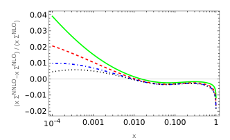
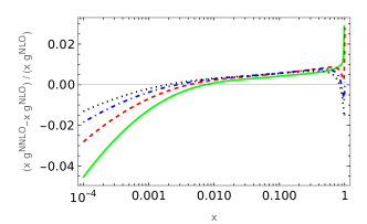
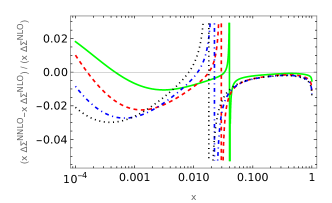
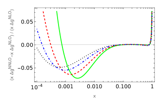
Figure 1: Ratios of the relative NNLO to NLO corrections of the singlet $(\Sigma)$ and gluon (G) distributions as functions of $x$. Upper panels: unpolarized case; lower panels: polarized case. $Q^{2}=10,10^{2},10^{3},10^{4}~{}\rm GeV^{2}$: dotted, dash-dotted, dashed, full lines. From Ref. [76].

One may now ask the question which order corrections are still important for current experimental precision analyses. Present day DIS data have an accuracy of up to O(1%). Future data, e.g. at the EIC[77], will reach at least this level. As shown in Figure 1 the NNLO corrections are not enough, in particular in the smaller $x$ and large $x$ regions. This applies also to the high luminosity data from the LHC. Therefore the four–loop splitting functions shall be calculated.

5 Massless Wilson Coefficients

For the massless Wilson coefficients the one–loop corrections were given in [78, 79]. The two–loop corrections were computed in Refs. [80, 45, 60] and the three–loop corrections were calculated in Refs. [63, 81, 65]. First color factor contributions of $O(N_{F}^{2})$ were computed recently in Ref. [82] at four loops. Up to the three–loop level all these quantities can be represented in terms of harmonic sums in Mellin space and the following 60 harmonic sums contribute[65], after algebraic reduction [83]

$$\{S_{1};S_{2},S_{-2};S_{3},S_{-3},S_{2,1},S_{-2,1};S_{4},S_{-4},S_{-2,2},S_{3,1},S_{-3,1},S_{2,1,1},S_{-2,1,1};S_{5},$$

$$S_{-5},S_{-2,3},S_{2,3},S_{2,-3},S_{-2,-3},S_{2,2,1},S_{-2,1,-2},S_{-2,2,1},S_{4,1},S_{-4,1},S_{2,1,-2},S_{3,1,1},$$

$$S_{-3,1,1},S_{2,1,1,1},S_{-2,1,1,1};S_{6},S_{-6},S_{-3,3},S_{4,2},S_{4,-2},S_{-4,2},S_{-4,-2},S_{5,1},S_{-5,1},$$

$$S_{-2,2,-2},S_{-2,2,2},S_{2,-3,1},S_{-2,3,1},S_{-3,1,-2},S_{-3,-2,1},S_{-3,2,1},S_{-4,1,1},S_{2,3,1},S_{3,1,-2},$$

$$S_{3,2,1},S_{4,1,1},S_{-2,-2,1,1},S_{-2,1,1,2},S_{-2,2,1,1},S_{2,-2,1,1},S_{2,2,1,1},S_{3,1,1,1},S_{-3,1,1,1},$$

$$S_{2,1,1,1,1},S_{-2,1,1,1,1}\}.$$ (19)

The harmonic sums are recursively defined by

$$S_{b,\vec{a}}(N)=\sum_{k=1}^{N}\frac{({\rm sign}(b))^{k}}{k^{|b|}}S_{\vec{a}}(k),~{}~{}S_{\emptyset}=1,b,a_{i}\in\mathbb{Z}\backslash\{0\},~{}~{}N\in\mathbb{N}\backslash\{0\}.$$ (20)

6 Massive Wilson Coefficients

The massive Wilson coefficients receive single mass and two–mass contributions (due to both charm and bottom quark corrections being present). We mainly will discuss asymptotic scales $Q^{2}\gg m_{Q}^{2}$ subsequently. In this case one obtains the following representation for the five contributing massive Wilson coefficients up to three–loop order[47]

$$L_{2,q}^{\sf NS}(N_{F}) = a_{s}^{2}\left[A_{qq,Q}^{{\sf NS},(2)}(N_{F})+\hat{C}^{{\sf NS},(2)}_{2,q}(N_{F})\right]$$ (21)

$$+ a_{s}^{3}\left[A_{qq,Q}^{{\sf NS},(3)}(N_{F})+A_{qq,Q}^{{\sf NS},(2)}(N_{F})C_{2,q}^{{\sf NS},(1)}(N_{F})+\hat{C}^{{\sf NS},(3)}_{2,q}(N_{F})\right]$$

$${\tilde{L}}_{2,q}^{\sf PS}(N_{F}) = a_{s}^{3}\left[~{}\tilde{A}_{qq,Q}^{{\sf PS},(3)}(N_{F})+A_{gq,Q}^{(2)}(N_{F})~{}~{}\tilde{C}_{2,g}^{(1)}(N_{F}+1)+\hat{\tilde{C}}^{{\sf PS},(3)}_{2,q}(N_{F})\right]$$ (22)

$${\tilde{L}}_{2,g}^{\sf S}(N_{F}) = a_{s}^{2}A_{gg,Q}^{(1)}(N_{F})\tilde{C}_{2,g}^{(1)}(N_{F}+1)$$ (23)

$$+ a_{s}^{3}\Bigl{[}~{}\tilde{A}_{qg,Q}^{(3)}(N_{F})+A_{gg,Q}^{(1)}(N_{F})~{}~{}\tilde{C}_{2,g}^{(2)}(N_{F}+1)+A_{gg,Q}^{(2)}(N_{F})$$

$$\hskip 14.22636pt~{}~{}\cdot\tilde{C}_{2,g}^{(1)}(N_{F}+1)+~{}A_{Qg}^{(1)}(N_{F})~{}~{}\tilde{C}_{2,q}^{{\sf PS},(2)}(N_{F}+1)+\hat{\tilde{C}}^{(3)}_{2,g}(N_{F})\Bigr{]}$$

$$H_{2,q}^{\sf PS}(N_{F}) = a_{s}^{2}\left[~{}A_{Qq}^{{\sf PS},(2)}(N_{F})+~{}\tilde{C}_{2,q}^{{\sf PS},(2)}(N_{F}+1)\right]$$ (24)

$$+ a_{s}^{3}\Bigl{[}~{}A_{Qq}^{{\sf PS},(3)}(N_{F})+~{}\tilde{C}_{2,q}^{{\sf PS},(3)}(N_{F}+1)+A_{gq,Q}^{(2)}(N_{F})~{}\tilde{C}_{2,g}^{(1)}(N_{F}+1)$$

$$\hskip 14.22636pt+A_{Qq}^{{\sf PS},(2)}(N_{F})~{}C_{2,q}^{{\sf NS},(1)}(N_{F}+1)\Bigr{]}$$

$$H_{2,g}^{\sf S}(N_{F}) = a_{s}\left[~{}A_{Qg}^{(1)}(N_{F})+~{}\tilde{C}^{(1)}_{2,g}(N_{F}+1)\right]$$ (25)

$$+ a_{s}^{2}\Bigl{[}~{}A_{Qg}^{(2)}(N_{F})+~{}A_{Qg}^{(1)}(N_{F})~{}C^{{\sf NS},(1)}_{2,q}(N_{F}+1)+~{}A_{gg,Q}^{(1)}(N_{F})$$

$$\hskip 14.22636pt~{}\cdot\tilde{C}^{(1)}_{2,g}(N_{F}+1)+~{}\tilde{C}^{(2)}_{2,g}(N_{F}+1)\Bigr{]}$$

$$+ a_{s}^{3}\Bigl{[}~{}A_{Qg}^{(3)}(N_{F})+~{}A_{Qg}^{(2)}(N_{F})~{}C^{{\sf NS},(1)}_{2,q}(N_{F}+1)+~{}A_{gg,Q}^{(2)}(N_{F})$$

$$\hskip 14.22636pt~{}\cdot\tilde{C}^{(1)}_{2,g}(N_{F}+1)+~{}A_{Qg}^{(1)}(N_{F})\left[C^{{\sf NS},(2)}_{2,q}(N_{F}+1)+~{}\tilde{C}^{{\sf PS},(2)}_{2,q}(N_{F}+1)\right]$$

$$\hskip 14.22636pt+~{}A_{gg,Q}^{(1)}(N_{F})~{}\tilde{C}^{(2)}_{2,g}(N_{F}+1)+~{}\tilde{C}^{(3)}_{2,g}(N_{F}+1)\Bigr{]},$$

where $\tilde{f}(N_{F})=f(N_{F})/N_{F},\hat{f}(N_{F})=f(N_{F}+1)-f(N_{F})$. Here $C_{i}$ are the respective contributions of the massless Wilson coefficients and $A_{ij}^{(k)}$ are the massive $k$-loop order OMEs. In the following we will deal with neutral–current interactions and the structure functions $F_{2}(x,Q^{2})$ and $F_{L}(x,Q^{2})$ [84]. Also for charged current processes higher order massive Wilson coefficients have been calculated. It turns out that beyond two–loop order several new mathematical quantities beyond the harmonic sums are contributing, cf. Section 9.

1 Single mass corrections

The one–loop corrections can be calculated for general values of $Q^{2}$ and were obtained in Refs. [85] in the unpolarized and polarized cases. The tagged–heavy flavor two–loop corrections were calculated numerically in Refs. [86]. Note that these corrections do not refer to the inclusive structure functions. These were calculated in the case of asymptotic scales $Q^{2}\gg m_{Q}^{2}$ in Refs. [27, 87, 88, 89, 90, 91]. The flavor non–singlet contributions can also be obtained in closed form for general values of $Q^{2}$, cf. [27, 87, 90]. This is also the case for the pure singlet contributions [92] and one may obtain a systematic expansions of the contributing power corrections of $O((m_{Q}^{2}/Q^{2})^{k})$. Here root–valued alphabets play a role and the results are given by incomplete elliptic integrals in part which are iterative integrals, unlike complete elliptic integrals. The analytic asymptotic two–loop results depend only on harmonic sums [52], as do the logarithmic scale corrections to three–loop order. The latter corrections were obtained in Refs. [93]. The three–loop corrections to the unpolarized asymptotic Wilson coefficients were computed in Refs. [94] and in the polarized case in Refs. [93, 95]

Massive OMEs determine also the transition matrix elements in the variable flavor scheme (VFNS). The corrections up to two–loop order were calculated in Refs. [97, 96, 91] and the single and two–mass VFNS were given in [97, 98, 91]. At three–loop order the massive OMEs beyond those contributing to the massive Wilson coefficients, were calculated in Refs. [93, 99, 66] for the unpolarized case and in Refs. [93, 100, 99] in the polarized case.

The transition relations in the single mass variable flavor number scheme[97] are given by

$$f_{k}(N_{F}+1,\mu^{2},m^{2},N)+f_{\overline{k}}(N_{F}+1,\mu^{2},m^{2},N)=$$ (26)

$$A_{qq,Q}^{\rm NS}\left(N_{F},\frac{\mu^{2}}{m^{2}},N\right)\cdot\bigl{[}f_{k}(N_{F},\mu^{2},N)+f_{\overline{k}}(N_{F},\mu^{2},N)\bigr{]}+\tilde{A}_{qq,Q}^{\rm PS}\left(N_{F},\frac{\mu^{2}}{m^{2}},N\right)$$

$$\cdot\Sigma(N_{F},\mu^{2},N)+\tilde{A}_{qg,Q}\left(N_{F},\frac{\mu^{2}}{m^{2}},N\right)\cdot G(N_{F},\mu^{2},N),$$

$$f_{Q}(N_{F}+1,\mu^{2},m^{2},N)+f_{\overline{Q}}(N_{F}+1,\mu^{2},m^{2},N)=$$ (27)

$${A}_{Qq}^{\rm PS}\left(N_{F},\frac{\mu^{2}}{m^{2}},N\right)\cdot\Sigma(N_{F},\mu^{2},N)+{A}_{Qg}\left(N_{F},\frac{\mu^{2}}{m^{2}},N\right)\cdot G(N_{F},\mu^{2},N)$$

$$\Sigma(N_{F}+1,\mu^{2},m^{2},N) = \Biggl{[}A_{qq,Q}^{\rm NS}\left(N_{F},\frac{\mu^{2}}{m^{2}},N\right)+N_{F}\tilde{A}_{qq,Q}^{\rm PS}\left(N_{F},\frac{\mu^{2}}{m^{2}},N\right)$$ (28)

$$+{A}_{Qq}^{\rm PS}\left(N_{F},\frac{\mu^{2}}{m^{2}},N\right)\Biggr{]}\cdot\Sigma(N_{F},\mu^{2},N)$$

$$+\Biggl{[}N_{F}\tilde{A}_{qg,Q}\left(N_{F},\frac{\mu^{2}}{m^{2}},N\right)+{A}_{Qg}\left(N_{F},\frac{\mu^{2}}{m^{2}},N\right)\Biggr{]}$$

$$\cdot G(N_{F},\mu^{2},N)$$

$$\Delta(N_{F}+1,\mu^{2},m^{2},N) = f_{k}(N_{F}+1,\mu^{2},N)+f_{\overline{k}}(N_{F}+1,\mu^{2},m^{2},N)$$ (29)

$$-\frac{1}{N_{F}+1}\Sigma(N_{F}+1,\mu^{2},m^{2},N)$$

$$G(N_{F}+1,\mu^{2},m^{2},N) = A_{gq,Q}\left(N_{F},\frac{\mu^{2}}{m^{2}},N\right)\cdot\Sigma(N_{F},\mu^{2},N)$$ (30)

$$+A_{gg,Q}\left(N_{F},\frac{\mu^{2}}{m^{2}},N\right)\cdot G(N_{F},\mu^{2},N)~{}.$$

In this way one may define also heavy quark parton densities $f_{Q(\overline{Q})}$ in the region $\mu^{2}\gg m_{Q}^{2}$. In the two–mass case one may separate the genuine two–mass contributions to $f_{c}$ and $f_{b}$, cf. [48].

2 Two-mass corrections

The two–mass corrections to the different massive OMEs, except that of $(\Delta)A_{Qg}^{(3)}$, can be calculated in terms of iterative integrals using square–root valued alphabets in which the real mass–ratio $\eta=m_{c}^{2}/m_{b}^{2}$ appears in $x$–space. In addition new special constants are contributing associated to these functions. The corrections, except those for $A_{Qg}^{(3)}$ in the unpolarized case, were calculated in Refs. [48, 101, 102]. In the polarized case the three–loop corrections were computed in Refs. [48, 103, 104]. The VFNS in the two–mass case has been given in [48]. It extends the one given in Section 1 and accounts for the fact that the mass ratio $m_{c}^{2}/m_{b}^{2}$ is not small.

7 Scheme-invariant evolution

The systematically and theoretically best way to measure the strong coupling constant in deep–inelastic scattering is due to the evolution of a given structure function itself. This requires specific experimental conditions, which were sometimes not available at some of the deep–inelastic facilities in the past. Having proton and deuteron data available in the same $(x,Q^{2})$–bins and performing the deuteron wave-function corrections allows to measure the following non–singlet structure functions

$$F_{2}^{\rm NS}(x,Q^{2}) = F_{2}^{p}-F_{2}^{d}=\frac{x}{6}C_{q}^{\rm NS+}\otimes[u+\bar{u}-d-\bar{d}],$$ (31)

$$xg_{1}^{\rm NS}(x,Q^{2}) = x(g_{1}^{p}-g_{1}^{d})=\frac{x}{6}\Delta C_{q}^{\rm NS+}\otimes[\Delta u+\Delta\bar{u}-\Delta d-\Delta\bar{d}],$$ (32)

see Ref. [105]. The massless and the massive non–singlet Wilson coefficients are available to three–loop order [63, 65, 107], including the two–mass corrections [48]. The scale evolution of the non–singlet combination of the parton distribution functions forming a single input density, requires four–loop anomalous dimensions. The investigation of moments shows, that these quantities can be extremely well constrained by a Padé–approximant of the lower order anomalous dimensions, implying a negligible theory error. The above equations can be rewritten in terms of evolution operators $(\Delta)E^{\rm NS}$

$$F_{2}^{\rm NS}(x,Q^{2}) = E^{\rm NS}(x,Q^{2},Q_{0}^{2})\otimes F_{2}^{\rm NS}(x,Q^{2}_{0}),$$ (33)

$$xg_{1}^{\rm NS}(x,Q^{2}) = x[\Delta E^{\rm NS}(x,Q^{2},Q_{0}^{2})\otimes g_{1}^{\rm NS}(x,Q^{2}_{0})].$$ (34)

Here the evolution operators can be analytically calculated in Mellin space in the analyticity region of $N\in\mathbb{C}$. The $x$–space result is then obtained by a single numerical contour integral around the singularities of the problem, cf. [108, 29]. Measuring the input structure functions at $Q_{0}^{2}$ with correlated errors, the evolution from $Q_{0}^{2}$ to the higher scales $Q^{2}$ depends only on a single parameter, the strong coupling constant $a_{s}(M_{Z}^{2})$ or the QCD–scale $\Lambda_{\rm QCD}$. The charm quark mass may be fixed within errors in this process and accounted for by error propagation. A measurement of this kind is proposed for further facilities, like the EIC [77] or the LHeC [109].

8 The Drell–Yan process

The Drell–Yan process of hadronic lepton pair production $pp\rightarrow\gamma^{*}/Z^{*}+X$ with subsequent leptonic decay of the virtual gauge bosons [110] or the associated charged current processes probe quark–antiquark initial states at leading order. Therefore this process is particularly sensitive to the sea quark distributions and yields complementary information to deep–inelastic scattering in disentangling the different light flavor distributions. The one–loop corrections to this process were calculated in Refs. [111] around 1980. The two–loop corrections have been completed 1990 in [112]. A subset of the Wilson coefficients is also related to the initial state QED corrections of $e^{+}e^{-}\rightarrow\gamma^{*}/Z^{*}+X$, for massive electrons in the limit $m_{e}^{2}/s\rightarrow 0$, where $s$ denotes the cms energy, cf. Ref. [113]. Like for all massless and massive two–loop single scale Wilson coefficients it has been shown in Ref. [114] that also in the case of the unpolarized and polarized Drell–Yan processes and Higgs–boson production only six functions are needed in Mellin $N$ space to describe these quantities. Here only harmonic sums [52] contribute. The three–loop corrections were calculated in Refs. [69]. Here also elliptic integrals contribute to the scattering cross section, if expressed in the variable $\hat{s}/s$, where $\hat{s}$ is the cms energy of the virtual gauge boson. In the experimental analysis one has to use differential distributions, such as encoded in the packages DYNNLO, FEWZ, MATRIX, MCFM [115].

9 Conclusions

Perturbative QCD has evolved significantly over the last 50 years and proven to be the correct theory of the strong interactions at high virtualities. While reviews like Ref. [116] in 1973 still were reluctant to evoke $SU_{3c}$ as part of the Standard Model, QCD allows now for highly precise predictions.

These analytic results required new mathematical and computer–algebraic technologies to be obtained. On the side of computer algebra we would like to mention in particular the IBP methods [53], Forcer [51], the packages Sigma [56] and HarmonicSums [117], the method of arbitrary high moments [54], and the method to perform the inverse Mellin transform without giving an explicit general $N$ expression [118]. At the mathematics side new developments have set in around 1998 with harmonic sums [52], generalized harmonic sums [119], cyclotomic harmonic sums [120], finite and infinite binomial sums [121, 122], related iterated integrals [75, 119, 120, 121], special numbers, e.g. Ref. [123], and methods related to ${}_{2}F_{1}$–solutions [124] and complete elliptic integrals [124, 125]. For a survey on these methods see Refs. [126]. Here the main question is: What can be integrated analytically and how? An important aspect in this context is anti-differentiation [127]. This development is still ongoing and we look forward for the new brilliant results to come.

Finally, we would like to comment on fundamental parameters of the Standard Model, such as $\alpha_{s}(M_{Z}^{2})$ and $m_{c}$, which can already be determined by the present high–precision data. These still will be improved when the calculation for all the three–loop heavy flavor corrections are completed. In earlier analyses we obtained in the non–singlet and singlet cases the following values for $\alpha_{s}(M_{Z}^{2})$

$$\alpha_{s}^{\rm N^{3}LO,NS}(M_{Z}^{2}) ~{}=~{} 0.1141\pm 0.0022 ~{}~{}[13]$$ , (35)

$$\alpha_{s}^{\rm N^{2}LO}(M_{Z}^{2}) ~{}=~{} 0.1140\pm 0.0009 ~{}~{}[12]$$ , (36)

and the charm quark mass

$$m_{c}(m_{c}) = 1.252\pm 0.018~{}\rm GeV.~{}~{}~{}[12].$$ (37)

Note that there is still a $0.07~{}\rm GeV$ theory error involved in the latter, which will be significantly reduced after the massive three–loop corrections are completely available. The result is very well compatible with the four–loop result based on $e^{+}e^{-}$ annihilation data

$$m_{c}(m_{c}) = 1.279\pm 0.008~{}\rm GeV.~{}~{}~{}[130].$$ (38)

Dedicated measurements at future high luminosity DIS facilities, like the EIC[77] and LHeC[109], are believed to improve these results further and to finally resolve the problem of still conflicting results on $\alpha_{s}(M_{Z}^{2})$ from different measurements [19, 131].

References

- [1] Y. Nambu, in: Preludes in Theoretical Physics, eds. A. De-Shalit, H. Fehsbach and L. van Hove (North-Holland, Amsterdam, 1966), pp. 133.
- [2] H. Fritzsch and M. Gell-Mann, Proceedings of 16th International Conference on High-Energy Physics, Batavia, Illinois, 6-13 Sep Vol. 2, J.D. Jackson, A. Roberts, R. Donaldson, eds., pp. 135 (1972) [hep-ph/0208010].
- [3] D.J. Gross and F. Wilczek, Phys. Rev. Lett. 30 (1973) 1343.
- [4] H.D. Politzer, Phys. Rev. Lett. 30 (1973) 1346.
- [5] H. Fritzsch, M. Gell-Mann and H. Leutwyler, Phys. Lett. B 47 (1973) 365.
- [6] M. J. G. Veltman SCHOONSCHIP, version 1, Dec. 1963.
- [7] G. ’t Hooft, Nucl. Phys. B 33 (1971) 173.
- [8] C.-N. Yang and R.L. Mills, Phys. Rev. 96 (1954) 191.
-
[9]
C. Bouchiat, J. Iliopoulos and P. Meyer,
Phys. Lett. B 38 (1972) 519;
D.J. Gross and R. Jackiw, Phys. Rev. D 6 (1972) 477. -
[10]
H. Abramowicz et al., [H1 and ZEUS],
Eur. Phys. J. C 75 (2015) 580;
R.D. Ball et al., [NNPDF], Eur. Phys. J. C 77 (2017) 663;
S. Bailey et al., Eur. Phys. J. C 81 (2021) 341;
A. Accardi et al., Eur. Phys. J. C 76 (2016) 471;
S. Amoroso et al., Acta Phys. Polon. B 53 (2022) A1. - [11] P. Jimenez-Delgado and E. Reya, Phys. Rev. D 89 (2014) 074049.
- [12] S. Alekhin, J. Blümlein, S. Moch and R. Placakyte, Phys. Rev. D 96 (2017) 014011.
- [13] J. Blümlein, H. Böttcher and A. Guffanti, Nucl. Phys. B 774 (2007) 182.
- [14] J. Blümlein and H. Böttcher, Phys. Lett. B 662 (2008) 336; arXiv:1207.3170 [hep-ph].
- [15] S. Alekhin, J. Blümlein and S. Moch, Phys. Rev. D 86 (2012) 054009.
-
[16]
W.K.H. Panofsky,
Proc. 14th International Conference on
High-Energy Physics, Vienna, 1968, J. Prentki and J. Steinberger, eds.,
(CERN, Geneva, 1968), pp. 23;
R.E. Taylor, Proc. 4th International Symposium on Electron and Photon Interactions at High Energies, Liverpool, 1969, (Daresbury Laboratory, 1969), eds. D.W. Braben and R.E. Rand, pp. 251; E.D. Bloom et al., Phys. Rev. Lett. 23 (1969) 930; M. Breidenbach et al., Phys. Rev. Lett. 23 (1969) 935. - [17] J.D. Bjorken, Phys. Rev. 179 (1969) 1547.
- [18] R.P. Feynman, in: Proceedings of 3rd International Conference on High Energy Collisions, Stony Brook, N.Y., 5-6 Sep 1969, pp 237.; Phys. Rev. Lett. 23 (1969) 1415; Photon-hadron interactions, (Benjamin, Reading, MA, 1972), 282 p.
-
[19]
S. Bethke et al.,
arXiv:1110.0016 [hep-ph];
S. Moch et al., arXiv:1405.4781 [hep-ph];
S. Alekhin, J. Blümlein and S.O. Moch, Mod. Phys. Lett. A 31 (2016) 1630023;
D. d’Enterria et al., arXiv:2203.08271 [hep-ph]. -
[20]
D.J. Gross and F. Wilczek,
Phys. Rev. D
8 (1973) 3633;
9 (1974) 980;
H. Georgi and H.D. Politzer, Phys. Rev. D 9 (1974) 416. - [21] S. Alekhin et al., Phys. Lett. B 720 (2013) 172.
-
[22]
K.G. Wilson,
Phys. Rev. 179 (1969) 1499;
R.A. Brandt and G. Preparata, Nucl. Phys. B 27 (1971) 541; Fortsch. Phys. 20 (1972) 571;
W. Zimmermann, in: Lectures on Elementary Particle Physics and Quantum Field Theory, Brandeis Summer Institute, 1 (MIT Press, Cambridge, 1970), pp. 395, Eds. S. Deser, M. Grisaru and H. Pendleton, and Ann. Phys. (NY) 77 (1973) 536;
Y. Frishman, Ann. Phys. (NY) 66 (1971) 373;
N.H. Christ, B. Hasslacher and A.H. Mueller, Phys. Rev. D 6 (1972) 3543. - [23] H.D. Politzer, Phys. Rept. 14 (1974) 129.
-
[24]
B. Geyer, D. Robaschik and E. Wieczorek,
Fortsch. Phys. 27 (1979) 75;
A.J. Buras, Rev. Mod. Phys. 52 (1980) 199;
E. Reya, Phys. Rept. 69 (1981) 195;
B. Lampe and E. Reya, Phys. Rept. 332 (2000) 1. - [25] J. Blümlein, Prog. Part. Nucl. Phys. 69 (2013) 28.
- [26] D.J. Gross and S.B. Treiman, Phys. Rev. D 4 (1971) 1059.
- [27] M. Buza et al., Nucl. Phys. B 472 (1996) 611.
-
[28]
H.D. Politzer, Nucl. Phys. B 129 (1977) 301;
D. Amati, R. Petronzio, and G. Veneziano, Nucl. Phys. B 140 (1978) 54; 146 (1978) 29;
S.B. Libby and G. Sterman, Phys. Rev. D 18 (1978) 3252, 4737;
A.H. Mueller, Phys. Rev. D 18 (1978) 3705;
J.C. Collins and G. Sterman, Nucl. Phys. B 185 (1981) 172;
J.C. Collins, D. Soper, and G. Sterman, Nucl. Phys. B 261 (1985) 104;
G.T. Bodwin, Phys. Rev. D 31 (1985) 2616. - [29] J. Blümlein and A. Vogt, Phys. Rev. D 58 (1998) 014020.
- [30] J. Blümlein, Lect. Notes Phys. 546 (2000) 42 and references therein.
-
[31]
K. Symanzik,
Commun. Math. Phys. 18 (1970) 227;
C.G. Callan, Jr., Phys. Rev. D 2 (1970) 1541. -
[32]
W.E. Caswell,
Phys. Rev. Lett. 33 (1974) 244;
D.R.T. Jones, Nucl. Phys. B 75 (1974) 531. -
[33]
O.V. Tarasov, A.A. Vladimirov and A.Y. Zharkov,
Phys. Lett. B 93 (1980) 429;
S.A. Larin and J.A.M. Vermaseren, Phys. Lett. B 303 (1993) 334;
K.G. Chetyrkin, M. Misiak and M. Münz, Nucl. Phys. B 518 (1998) 473. -
[34]
T. van Ritbergen, J.A.M. Vermaseren and S.A. Larin,
Phys. Lett. B 400 (1997) 379;
M. Czakon, Nucl. Phys. B 710 (2005) 485. -
[35]
P.A. Baikov, K.G. Chetyrkin and J.H. Kühn,
Phys. Rev. Lett. 118 (2017) 082002;
F. Herzog et al., JHEP 02 (2017) 090;
T. Luthe et al., JHEP 10 (2017) 166. - [36] E. Egorian and O.V. Tarasov, Teor. Mat. Fiz. 41 (1979) 26 and Erratum.
- [37] J.A.M. Vermaseren, S.A. Larin and T. van Ritbergen, Phys. Lett. B 405 (1997) 327.
- [38] K.G. Chetyrkin, Nucl. Phys. B 710 (2005) 499.
- [39] K.G. Chetyrkin et al., JHEP 1710 (2017) 179 Addendum: [JHEP 1712 (2017) 006].
- [40] T. Luthe et al., JHEP 1701 (2017) 081.
-
[41]
R. Tarrach,
Nucl. Phys. B 183 (1981) 384;
O. Nachtmann and W. Wetzel, Nucl. Phys. B 187 (1981) 333;
N. Gray et al., Z. Phys. C 48, (1990) 673;
D.J. Broadhurst, N. Gray and K. Schilcher, Z. Phys. C 52 (1991) 111;
K.G. Chetyrkin and M. Steinhauser, Nucl. Phys. B 573 (2000) 617; Phys. Rev. Lett. 83 (1999) 4001;
K. Melnikov and T. van Ritbergen, Phys. Lett. B 482 (2000) 99; Nucl. Phys. B 591 (2000) 515;
P. Marquard et al., Nucl. Phys. B 773 (2007) 1; Phys. Rev. Lett. 114 (2015) 142002; Phys. Rev. D 97 (2018) 054032; 94 (2016) 074025. - [42] J. Blümlein and N. Kochelev, Nucl. Phys. B 498 (1997) 285.
-
[43]
S.G. Gorishnii et al., Comput. Phys. Commun. 55 (1989) 381;
S.A. Larin, F.V. Tkachov and J.A.M. Vermaseren, NIKHEF-H-91-18. - [44] M. Steinhauser, Comput. Phys. Commun. 134 (2001) 335.
- [45] S.A. Larin and J.A.M. Vermaseren, Z. Phys. C 57 (1993) 93.
-
[46]
S.A. Larin, T. van Ritbergen and J.A.M. Vermaseren,
Nucl. Phys. B 427 (1994) 4;
S.A. Larin et al., Nucl. Phys. B 492 (1997) 338;
A. Retey and J.A.M. Vermaseren, Nucl. Phys. B 604 (2001) 281;
J. Blümlein and J.A.M. Vermaseren, Phys. Lett. B 606 (2005) 130. - [47] I. Bierenbaum, J. Blümlein and S. Klein, Nucl. Phys. B 820 (2009) 417.
- [48] J. Ablinger et al., F. Wißbrock, Nucl. Phys. B 921 (2017) 585.
-
[49]
P.A. Baikov and K.G. Chetyrkin,
Nucl. Phys. (Proc. Suppl.) 160 (2006) 76;
V.N. Velizhanin, Nucl. Phys. B 860 (2012) 288; Int. J. Mod. Phys. A 35 (2020) 2050199;
P.A. Baikov, K.G. Chetyrkin and J.H. Kühn, Nucl. Phys. (Proc. Suppl.) 261-262 (2015) 3;
S. Moch et al., Phys. Lett. B 825 (2022) 136853;
G. Falcioni et al., Phys. Lett. B 842 (2023) 137944. -
[50]
J. Davies et al., Nucl. Phys. B 915 (2017) 335;
S. Moch et al., JHEP 10 (2017) 041. - [51] B. Ruijl, T. Ueda and J.A.M. Vermaseren, Comput. Phys. Commun. 253 (2020) 107198.
-
[52]
J.A.M. Vermaseren,
Int. J. Mod. Phys. A 14 (1999) 2037;
J. Blümlein and S. Kurth, Phys. Rev. D 60 (1999) 014018. -
[53]
K.G. Chetyrkin and F.V. Tkachov,
Nucl. Phys. B 192 (1981) 159–204;
S. Laporta, Int. J. Mod. Phys. A 15 (2000) 5087–5159 [hep-ph/0102033];
P. Marquard and D. Seidel, The Crusher algorithm, unpublished;
A. von Manteuffel and C. Studerus, arXiv:1201.4330 [hep-ph]. -
[54]
J. Blümlein and C. Schneider,
Phys. Lett. B 771 (2017) 31;
J. Blümlein, P. Marquard and C. Schneider, PoS (RADCOR2019) 078. -
[55]
M. Kauers, Guessing Handbook, JKU Linz, Technical Report RISC 09–07;
J. Blümlein et al., Comput. Phys. Commun. 180 (2009) 2143;
M. Kauers, M. Jaroschek, and F. Johansson, in: Computer Algebra and Polynomials, Editors: J. Gutierrez, J. Schicho, M. Weimann, Eds.. Lecture Notes in Computer Science 8942 (Springer, Berlin, 2015) 105. - [56] C. Schneider, Sém. Lothar. Combin. 56 (2007) 1 article B56b; in: Computer Algebra in Quantum Field Theory: Integration, Summation and Special Functions Texts and Monographs in Symbolic Computation eds. C. Schneider and J. Blümlein (Springer, Wien, 2013) 325; J. Phys. Conf. Ser. 523 (2014) 012037.
-
[57]
K. Sasaki,
Prog. Theor. Phys. 54 (1975) 1816;
M.A. Ahmed and G.G. Ross, Phys. Lett. B 56 (1975) 385. - [58] G. Parisi, An Introduction to Scaling Violations, LNF-76-25-P, Int. Meeting on Neutrino Physics, Flaine, March 6–12, 1976; G. Altarelli and G. Parisi, Nucl. Phys. B 126 (1977) 298.
-
[59]
E.G. Floratos, D.A. Ross and C.T. Sachrajda,
Nucl. Phys. B 129 (1977) 66
[Erratum B 139 (1978) 545];
Nucl. Phys. B 152 (1979) 493;
A. Gonzalez-Arroyo, C. Lopez and F.J. Yndurain, Nucl. Phys. B 153 (1979) 161; Nucl. Phys. B 159 (1979) 512;
G. Curci, W. Furmanski and R. Petronzio, Nucl. Phys. B 175 (1980) 27;
W. Furmanski and R. Petronzio, Phys. Lett. B 97 (1980) 437;
E.G. Floratos, R. Lacaze and C. Kounnas, Phys. Lett. B 98 (1981) 89; Nucl. Phys. B 192 (1981) 417; Phys. Lett. B 98 (1981) 285;
A. Gonzalez-Arroyo and C. Lopez, Nucl. Phys. B 166 (1980) 429;
R. Hamberg and W.L. van Neerven, Nucl. Phys. B 379 (1992) 143;
R.K. Ellis and W. Vogelsang, hep-ph/9602356;
Y. Matiounine, J. Smith and W.L. van Neerven, Phys. Rev. D 58 (1998) 076002 57 (1998) 6701;
J. Blümlein et al., Nucl. Phys. B 980 (2022) 115794 - [60] S. Moch and J.A.M. Vermaseren, Nucl. Phys. B 573 (2000) 853.
-
[61]
R. Mertig and W.L. van Neerven,
Z. Phys. C 70 (1996) 637;
W. Vogelsang, Phys. Rev. D 54 (1996) 2023; Nucl. Phys. B 475 (1996) 47. - [62] S. Moch, J.A.M. Vermaseren and A. Vogt, Nucl. Phys. B 688 (2004) 101; 691 (2004) 129.
- [63] J.A.M. Vermaseren, A. Vogt and S. Moch, Nucl. Phys. B 724 (2005) 3.
- [64] J. Blümlein et al., Nucl. Phys. B 971 (2021) 115542.
- [65] J. Blümlein et al., JHEP 11 (2022) 156 and [arXiv:2208.14325 [hep-ph]].
- [66] J. Ablinger et al., Nucl. Phys. B 882 (2014) 263.
- [67] J. Ablinger et al., Nucl. Phys. B 922 (2017) 1.
-
[68]
C. Anastasiou et al., Phys. Rev. Lett. 114 (2015) 212001;
B. Mistlberger, JHEP 05 (2018) 028;
M.X. Luo et al., Phys. Rev. Lett. 124 (2020) 092001 JHEP 06 (2021) 115;
M.A. Ebert, B. Mistlberger and G. Vita, JHEP 09 (2020) 146; 09 (2020) 143;
D. Baranowski et al. JHEP 02 (2023) 073. - [69] C. Duhr, F. Dulat and B. Mistlberger, Phys. Rev. Lett. 125 (2020) 172001; JHEP 11 (2020) 143.
- [70] T. Gehrmann, A. von Manteuffel and T.Z. Yang, JHEP 04 (2023) 041.
- [71] S. Moch, J.A.M. Vermaseren and A. Vogt, Nucl. Phys. B 889 (2014) 351.
- [72] A. Behring et al., Nucl. Phys. B 948 (2019) 114753.
- [73] J. Blümlein et al., JHEP 01 (2022) 193.
- [74] T. Gehrmann et al., in preparation.
- [75] E. Remiddi and J.A.M. Vermaseren, Int. J. Mod. Phys. A 15 (2000) 725.
- [76] M. Saragnese, PhD Thesis, Univ. Hamburg, 2022 [arXiv:2208.06145 [hep-ph]].
- [77] D. Boer et al., arXiv:1108.1713 [nucl-th].
- [78] W. Furmanski and R. Petronzio, Z. Phys. C 11 (1982) 293 and Refs. therein.
- [79] G. T. Bodwin and J. -W. Qiu, Phys. Rev. D 41 (1990) 2755.
-
[80]
E.B. Zijlstra and W.L. van Neerven,
Phys. Lett. B 273 (1991) 476;
B 272 (1991) 127;
Nucl. Phys. B 383 (1992) 525;
Phys. Lett. B 297 (1992) 377;
Nucl. Phys. B 417 (1994) 61;
[Errata: 426 (1994) 245; 773 (2007), 105;
501 (1997) 599];
D.I. Kazakov and A.V. Kotikov, Nucl. Phys. B 307 (1988) 721 [Erratum B 345 (1990) 299];
D.I. Kazakov et al., Phys. Rev. Lett. 65 (1990) 1535 [Erratum 65 (1990) 2921];
J. Sanchez Guillen et al., Nucl. Phys. B 353 (1991) 337;
A. Vogt et al. Nucl. Phys. B (Proc. Suppl.) 183 (2008) 155. - [81] S. Moch, J.A.M. Vermaseren and A. Vogt, Nucl. Phys. B 813 (2009) 220.
- [82] A. Basdew-Sharma et al., JHEP 03 (2023) 183.
- [83] J. Blümlein, Comput. Phys. Commun. 159 (2004) 19.
- [84] J. Blümlein et al., Nucl. Phys. B 755 (2006) 272.
-
[85]
E. Witten,
Nucl. Phys. B 104 (1976) 445;
J. Babcock, D.W. Sivers and S. Wolfram, Phys. Rev. D 18 (1978) 162;
M.A. Shifman, A.I. Vainshtein and V.I. Zakharov, Nucl. Phys. B 136 (1978) 157;
J.P. Leveille and T.J. Weiler, Nucl. Phys. B 147 (1979) 147;
M. Glück, E. Hoffmann and E. Reya, Z. Phys. C 13 (1982) 119;
A.D. Watson, Z. Phys. C 12 (1982) 123;
M. Glück, E. Reya and W. Vogelsang, Nucl. Phys. B 351 (1991) 579;
W. Vogelsang, Z. Phys. C 50 (1991) 275. -
[86]
E. Laenen et al., Nucl. Phys. B 392 (1993) 162;
229;
S. Riemersma, J. Smith and W.L. van Neerven, Phys. Lett. B 347 (1995) 143;
S.I. Alekhin and J. Blümlein, Phys. Lett. B 594 (2004) 299;
F. Hekhorn and M. Stratmann, Phys. Rev. D 98 (2018) 014018. - [87] M. Buza et al., Nucl. Phys. B 485 (1997) 420.
- [88] I. Bierenbaum, J. Blümlein and S. Klein, Nucl. Phys. B 780 (2007) 40.
- [89] I. Bierenbaum et al., Nucl. Phys. B 803 (2008) 1.
- [90] J. Blümlein, G. Falcioni and A. De Freitas, Nucl. Phys. B 910 (2016) 568.
- [91] I. Bierenbaum et al., Nucl. Phys. B 988 (2023) 116114.
-
[92]
J. Blümlein et al., Nucl. Phys. B 945 (2019) 114659;
J. Blümlein, C. Raab and K. Schönwald, Nucl. Phys. B 948 (2019) 114736. -
[93]
A. Behring et al., Eur. Phys. J. C 74 (2014) 3033;
J. Blümlein et al., Phys. Rev. D 104 (2021) 034030. -
[94]
J. Ablinger et al., Nucl. Phys. B 844 (2011) 26; Nucl. Phys. B 886 (2014) 733; Nucl. Phys. B 890 (2014) 48;
J. Blümlein et al., PoS (QCDEV2017) 031. - [95] J. Ablinger et al., Nucl. Phys. B 953 (2020) 114945.
- [96] I. Bierenbaum, J. Blümlein and S. Klein, Phys. Lett. B 672 (2009) 401.
- [97] M. Buza et al., Eur. Phys. J. C 1 (1998) 301.
- [98] J. Blümlein et al., Phys. Lett. B 782 (2018) 362.
- [99] J. Ablinger et al., JHEP 12 (2022) 134.
- [100] A. Behring et al., Nucl. Phys. B 964 (2021) 115331.
- [101] J. Ablinger et al., Nucl. Phys. B 932 (2018) 129.
- [102] J. Ablinger et al., Nucl. Phys. B 927 (2018) 339.
- [103] J. Ablinger et al., Nucl. Phys. B 955 (2020) 115059.
- [104] J. Ablinger et al., Nucl. Phys. B 952 (2020) 114916.
- [105] J. Blümlein and M. Saragnese, Phys. Lett. B 820 (2021) 136589.
-
[106]
G. Grunberg,
Phys. Rev. D 29 (1984) 2315;
S. Catani, Z. Phys. C 75 (1997) 665;
J. Blümlein, V. Ravindran and W.L. van Neerven, Nucl. Phys. B 586 (2000) 349;
J. Blümlein and A. Guffanti, Nucl. Phys. B Proc. Suppl. 152 (2006) 87. - [107] J. Ablinger et al., Nucl. Phys. B 886 (2014) 733.
- [108] M. Diemoz et al., Z. Phys. C 39 (1988) 21.
-
[109]
J.L. Abelleira Fernandez et al., J. Phys. G 39 (2012) 075001;
P. Agostini et al., J. Phys. G 48 (2021) 110501. - [110] S.D. Drell and T.M. Yan, Phys. Rev. Lett. 25 (1970) 316; [Erratum: 25 (1970) 902].
-
[111]
G. Altarelli, R.K. Ellis and G. Martinelli,
Nucl. Phys. B 143 (1978) 521
[Erratum: 146 (1978) 544];
J. Abad and B. Humpert, Phys. Lett. B 78 (1978) 627 [Erratum: B 80 (1979) 433]; Phys. Lett. B 80 (1979) 286;
J. Kubar-Andre and F.E. Paige, Phys. Rev. D 19 (1979) 221;
K. Harada, T. Kaneko and N. Sakai, Nucl. Phys. B 155 (1979) 169 [Erratum: 165 (1980) 545];
B. Humpert and W. L. Van Neerven, Phys. Lett. B 84 (1979) 327 [Erratum: B 85 (1979) 471]; Phys. Lett. B 89 (1979) 69 Nucl. Phys. B 184 (1981) 225;
J. Kubar et al., Nucl. Phys. B 175 (1980) 251. -
[112]
R. Hamberg, W.L. van Neerven and T. Matsuura,
Nucl. Phys. B 359 (1991) 343; [Erratum: B 644 (2002), 403];
R.V. Harlander and W.B. Kilgore, Phys. Rev. Lett. 88 (2002) 201801. - [113] J. Blümlein et al., Nucl. Phys. B 956 (2020) 115055.
- [114] J. Blümlein and V. Ravindran, Nucl. Phys. B 716 (2005) 128.
-
[115]
S. Catani and M. Grazzini,
Phys. Rev. Lett. 98 (2007) 222002;
S. Catani et al., Phys. Rev. Lett. 103 (2009) 082001;
Y. Li and F. Petriello, Phys. Rev. D 86 (2012) 094034;
R. Gavin et al., Comput. Phys. Commun. 184 (2013) 208;
M. Grazzini, S. Kallweit and M. Wiesemann, Eur. Phys. J. C 78 (2018) 537;
J. Campbell and T. Neumann, JHEP 12 (2019) 034;
S. Alekhin et al., Eur. Phys. J. C 81 (2021) 573. - [116] E.S. Abers and B.W. Lee, Phys. Rept. 9 (1973) 1.
- [117] J. Ablinger, arXiv:1011.1176 [math-ph]; arXiv:1305.0687 [math-ph]; and Refs. given in Ref. [99].
- [118] A. Behring, J. Blümlein and K. Schönwald, JHEP (2023) in print [arXiv:2303.05943 [hep-ph]].
-
[119]
J.M. Borwein et al., Trans. Am. Math. Soc. 353 (2001) 907;
S. Moch, P. Uwer and S. Weinzierl, J. Math. Phys. 43 (2002) 3363;
J. Ablinger, J. Blümlein and C. Schneider, J. Math. Phys. 54 (2013) 082301. - [120] J. Ablinger, J. Blümlein and C. Schneider, J. Math. Phys. 52 (2011) 102301.
- [121] J. Ablinger et al., J. Math. Phys. 55 (2014) 112301.
-
[122]
A.I. Davydychev and M.Y. Kalmykov,
Nucl. Phys. B 699 (2004) 3;
S. Weinzierl, J. Math. Phys. 45 (2004) 2656. - [123] J. Blümlein, D.J. Broadhurst and J.A.M. Vermaseren, Comput. Phys. Commun. 181 (2010) 582.
- [124] J. Ablinger et al., J. Math. Phys. 59 (2018) 062305.
-
[125]
D.J. Broadhurst,
Z. Phys. C 47 (1990) 115;
D.J. Broadhurst, J. Fleischer and O.V. Tarasov, Z. Phys. C 60 (1993) 287;
S. Bloch and P. Vanhove, J. Num. Theor. 148 (2015) 328;
L. Adams, C. Bogner and S. Weinzierl, J. Math. Phys. 57 (2016) 032304;
E. Remiddi and L. Tancredi, Nucl. Phys. B 907 (2016) 400;
L. Adams and S. Weinzierl, Commun. Num. Theor. Phys. 12 (2018) 193;
J. Broedel et al., JHEP 05 (2019) 120;
J. Blümlein, C. Schneider and P. Paule, Proceedings, KMPB Conference: Elliptic Integrals, Elliptic Functions and Modular Forms in Quantum Field Theory, Zeuthen, Germany, October 23–26, 2017, (Springer, Berlin, 2019). -
[126]
J. Blümlein and C. Schneider,
Int. J. Mod. Phys. A 33 (2018) 1830015;
S. Weinzierl, Feynman Integrals, (Springer, Berlin 2022). - [127] J. Blümlein and C. Schneider, Eds., Anti-Differentiation and the Calculation of Feynman Amplitudes, (Springer, Berlin, 2021).
- [128] R.S. Thorne, PoS (DIS2013) 042.
- [129] S. Dulat et al., Phys. Rev. D 93 (2016) 033006.
- [130] K.G. Chetyrkin et al., Phys. Rev. D 96 (2017) 116007.
- [131] S. Bethke, contribution to this volume.