Energy-Efficient UAV-Assisted IoT Data Collection via TSP-Based Solution Space Reduction

Abstract

This paper presents a wireless data collection framework that employs an unmanned aerial vehicle (UAV) to efficiently gather data from distributed IoT sensors deployed in a large area. Our approach takes into account the non-zero communication ranges of the sensors to optimize the flight path of the UAV, resulting in a variation of the Traveling Salesman Problem (TSP). We prove mathematically that the optimal waypoints for this TSP-variant problem are restricted to the boundaries of the sensor communication ranges, greatly reducing the solution space. Building on this finding, we develop a low-complexity UAV-assisted sensor data collection algorithm, and demonstrate its effectiveness in a selected use case where we minimize the total energy consumption of the UAV and sensors by jointly optimizing the UAV’s travel distance and the sensors’ communication ranges.

I Introduction

Wireless sensor networks (WSNs) are typically made up of inexpensive Internet of Things (IoT) sensor nodes that have been spatially distributed in order to detect and collect environmental and physical data sets for various applications including smart farming, battlefield monitoring, smart healthcare, and disaster warning. However, these IoT sensor nodes may not be able to form a network (i.e., WSN) if the inter-node distances are long and the communication range of nodes is limited. Then, unmanned aerial vehicles (UAVs) can be used as data mules in transferring data swiftly over long distances, opportunistically [1] [2]. Such a scenario would require a UAV to dynamically move towards IoT sensor nodes, collect data and transmit this data to the base station (BS) or other sensor nodes which are typically outside the coverage radius. The employment of UAVs for data collecting is also motivated by the rising adaptability of 5G networks and wide bandwidth availability [3] [4], which means that UAVs may operate at various altitudes and download enormous amounts of data from sensor nodes.

In particular, with the advancement of wireless capabilities in UAVs in recent years, they have been used as data mules for data collection from sensor nodes. UAVs can be deployed to collect data from each sensor node with an energy-efficient approach. To begin data collection, a UAV must move close enough to a sensor node and does not need to hover directly over the sensor node; as a result, the link distance between the UAV and the sensor node is greatly reduced. We borrow the term “data mule” from [5], a mobile object that can be used for data collection. The UAV’s capabilities are not limited to data collection; it can also be used for surveillance and other tasks.

I-A Traveling Salesman Problem for UAV Path Planning

The Traveling Salesman Problem (TSP) can be considered for UAV path planning [6] [7]. Since the TSP is a nondeterministic polynomial (NP)-hard problem, there are a number of heuristic methods such as simulated annealing [8], genetic algorithm [9], and so on. While UAV path planning can be seen as a TSP, it would be necessary to take into consideration the communication range of the sensor node and the UAV. Since a UAV can simply pass through any point specified by the sensor node’s communication range (also known as executable area or neighborhood) to collect data from the sensor, the TSP with neighborhoods (TSPN), which was introduced by [10], can be considered for UAV path planning. TSP with a varying neighborhood size is studied in [11], [12], while TSP with circular neighborhoods is studied in [13].In [14], the authors proposed a method for efficient data collection in WSNs using a resource-constrained mobile sink. The approach modeled the TSP for minimizing the distance that the mobile sink has to travel and utilized reduce methods to develop a computationally efficient approach for data collection.

I-B Main Contributions and Organization

In this paper, while a TSPN is considered to model data collection by a UAV as in [12] [13], the main contributions are as follows:

• It is rigorously proved that there exists at least one optimal collection point that lies on the boundary of each communication region of a node or the intersection of overlapped communication region of closely located nodes (to the best of our knowledge, this proof was previously unavailable), which can allow us to significantly reduce the travel distance in UAV path planning.

• Through a case study, an optimization problem is studied to decide an optimal communication range when minimizing a weighted energy consumption subject to key constraints.

II System Model

Suppose that there are $N$ ground nodes with measurements or data to send, which are distributed over a certain (remote) area. Each ground node has a limited energy source and its communication range is limited, meaning that each node is unable to transmit its signals to an access point connected to a backbone network. Thus, we consider the case that a UAV is used to collect measurements from ground nodes.

A UAV leaves a certain initial location, denoted by ${\bf u}_{0}$, and, after visiting $N$ nodes, arrives at another location, denoted by ${\bf u}_{N+1}$, which is referred to as the terminal location. The location of ground node $n$ is denoted by ${\bf v}_{n}$, $n=1,\ldots,N$. The communication region of ground node $n$ is characterized by the following disc:

$${\cal V}_{n}=\{{\bf x}:||{\bf v}_{n}-{\bf x}||_{2}\leq r\},$$ (1)

which is referred to as the communication region of ground node $n$, where $r$ denotes the communication range. For each node, there is a possibility of intersecting communication region denoted as

$$\mathcal{N}(\mathcal{V}_{n})=\{\forall j\in N\mid\mathcal{V}_{j}\cap\mathcal{V}_{n}\neq\varnothing,~{}j\neq n\}$$ (2)

It is assumed that the initial and terminal locations do not belong to any of the communication regions of ground nodes, i.e., ${\bf u}_{0},{\bf u}_{N+1}\notin\bigcup_{n}{\cal V}_{n}$.

The communication range $r$ in (1) is determined by the transmit power $P_{\rm g}$ of a ground node. Then, the signal-to-noise ratio (SNR) at a UAV at a distance $r$ becomes

$${\sf SNR}(r)=\frac{P_{\rm g}r^{-\eta}}{N_{0}},$$ (3)

where $\eta$ and $N_{0}$ denote the path loss exponent and the noise variance at UAV, respectively. The corresponding achievable rate becomes $C(r)=\log_{2}(1+{\sf SNR}(r))$.

For each node, consider a ball with radius $r$, which characterizes the communication region. In this case, if the altitude of UAV is $h\ (\leq r)$, (1) can be modified as ${\cal V}_{n}=\{{\bf x}:||{\bf v}_{n}-{\bf x}||_{2}\leq\bar{r}\}$, where $\bar{r}=\sqrt{r^{2}-h^{2}}$. In order to maximize the area of the communication region, the altitude of UAV, $h$, can be as low as possible, i.e., $h=0$. In this case, according to [15], there might be obstacles between the UAV and a ground node, which result in non-line-of-sight (NLoS) paths. Thus, the SNR can be lower than that in (3) due to longer propagation paths and small-scale fading. While it would be worth to study the impact of $h$ on the performance, in this paper, we assume that $h$ is greater than a certain non-zero threshold so that the UAV can have a line-of-sight (LoS) to a ground node and the SNR in (3) is valid.

If the number of bits to send to the UAV from a ground node is $B$, the UAV needs to fly within the communication region for a time of $T_{\rm c}=\frac{B}{W\log_{2}(1+{\sf SNR}(r))}$, where $W$ is the bandwidth of the signal transmission from a ground node to the UAV.

Example 1

Suppose that the speed of a drone (as a UAV) is 60 km/hr, while $W=22$ MHz and ${\sf SNR}(r)=6$ dB. If $B=10^{4}$ bits, $T_{\rm c}$ becomes $0.196\times 10^{-3}$ sec or $0.196$ msec. In this case, within the communication region, the UAV only needs to move $3.27\times 10^{-3}$ meters. If $r$ is a few ten meters, the moving distance of the UAV for receiving data from a ground node is relatively short, meaning that the UAV does not need to travel deep into the communication region, but only crosses the boundary.

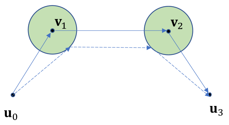
Figure 1: Two different UAV trajectories when $N=2$.

Example 2

In order to see the impact of a non-zero communication range on the travel distance, we consider an example with $N=2$. As shown in Fig. 1, the trajectory shown by solid lines is the case that the UAV needs to visit the exact locations of two ground nodes, ${\bf v}_{1}$ and ${\bf v}_{2}$. On the other hand, the trajectory shown by dashed lines is the case that the UAV just crosses the boundaries of the communication regions of two ground nodes. Clearly, the latter case leads to a shorter travel distance, from which it is expected that the UAV’s travel distance decreases with $r$.

III Problem Formulation

In this section, we focus on the problem for a UAV that collects data from multiple ground nodes with a non-zero communication range with the following key assumptions:

• The number of bits, $B$, that a ground node is to send to the UAV is sufficiently small (as illustrated in Example 1) so that the data collection time can be ignored when the UAV travels within the communication region.

• The altitude of the UAV is fixed. As a result, the communication region is characterized by a 2-dimensional circle as shown in (1).

For convenience, let ${\bf u}_{n}\in{\cal V}_{n}$ be any location that the UAV must pass through to collect measurements or data from ground node $n$, which is referred to as the $n$th collection point. In addition, let $d_{m,n}=||{\bf u}_{m}-{\bf u}_{n}||_{2}$. There are $N!$ possible paths that the UAV can take. For a given path, say path $m\in\{1,\ldots,N!\}$, let $m(n)$ denote the index of the ground node that the UAV visits after visiting $n-1$ ground nodes. Then, the total travel distance of the UAV according to path $m$ is $D_{m}=d_{0,m(1)}+d_{m(1),m(2)}+\cdots+d_{m(N),N+1}$. For path $m$, the collection points can be optimized as follows:

$$\{{\bf u}_{m(1)}^{\ast},\ldots,{\bf u}_{m(N)}^{\ast}\}=\operatorname*{\arg\!\min}_{{\bf u}_{m}(n),\ n=1,\ldots,N}D_{m}$$ (4)

$$\mbox{subject to}\ {\bf u}_{m(n)}\in{\cal V}_{m(n)},\ n=1,\ldots,N,$$ (5)

which is referred to as the inner optimization problem. Note that due to Assumption of A1, the UAV does not need to hover over the communication regions and continues to fly at a constant speed. Thus, if the energy consumption of UAV is proportional to the travel distance, (5) can also be seen as the minimization of UAV energy consumption.

There is also the outer optimization problem that chooses the optimal path with the shortest distance. As a result, the optimization problem can be given as

$$m^{\ast} =\operatorname*{\arg\!\min}_{m\in\{1,\ldots,N!\}}D_{m}^{\ast},$$ (6)

where $D_{m}^{\ast}$ is the minimum total distance for given path $m$, which can be obtained by solving (5).

IV Optimization Techniques

IV-A Main Results

In this subsection, we focus on the inner optimization problem and present the main results that can lower the computational complexity.

Lemma 1

For given two points, denoted by ${\bf a}$ and ${\bf b}$, outside of a closed convex set ${\cal V}$, suppose that the straight line between two points does not intersect ${\cal V}$ (if it does, the solution can be readily obtained). Let

$${\bf z}=\operatorname*{\arg\!\min}_{{\bf x}\in{\cal V}}||{\bf x}-{\bf a}||+||{\bf x}-{\bf b}||.$$

Then, ${\bf z}\in\bar{\cal V}$, where $\bar{\cal V}$ is the boundary of ${\cal V}$.

Proof:

Consider the point ${\bf t}$ on the straight line passing through ${\bf a}$ and ${\bf b}$ that satisfies the following: $({\bf t}-{\bf b})^{\rm T}({\bf t}-{\bf z})=0$. That is ${\bf t}-{\bf b}$ is orthogonal to ${\bf t}-{\bf z}$. We now assume that ${\bf z}$ is an interior point of ${\cal V}$. By showing that this interior point ${\bf z}$ cannot be the solution of (1), we can prove that ${\bf z}$ has to be on the boundary.

By the definition of ${\bf z}$, $||{\bf a}-{\bf z}||+||{\bf b}-{\bf z}||$ should be the minimum. Consider another point ${\bf y}$ in ${\cal V}$, which is given by ${\bf y}={\bf z}+\epsilon{\bf w}\in{\cal V}$, where $\epsilon>0$ and ${\bf w}=\frac{{\bf t}-{\bf z}}{||{\bf t}-{\bf z}||}$ (thanks to ${\cal V}$ is a closed convex set). Then, there exists $\epsilon$ such that

$$||{\bf t}-{\bf y}||=||{\bf t}-({\bf z}+\epsilon{\bf w})||=||(1-\epsilon^{\prime})({\bf t}-{\bf z})||<||{\bf t}-{\bf z}||,$$

where $\epsilon^{\prime}=\frac{\epsilon}{||{\bf t}-{\bf z}||}<1$. From this, by the Pythagorean theorem, we can also show that

$$||{\bf a}-{\bf z}||^{2} =||{\bf a}-{\bf t}||^{2}+||{\bf t}-{\bf z}||^{2}>||{\bf a}-{\bf t}||^{2}+||{\bf t}-{\bf y}||^{2}$$

$$\geq||{\bf a}-{\bf y}||^{2}$$

$$||{\bf b}-{\bf z}||^{2} =||{\bf b}-{\bf t}||^{2}+||{\bf t}-{\bf z}||^{2}>||{\bf b}-{\bf t}||^{2}+||{\bf t}-{\bf y}||^{2}$$

$$\geq||{\bf b}-{\bf y}||^{2}.$$

This shows that $||{\bf a}-{\bf z}||+||{\bf b}-{\bf z}||>||{\bf a}-{\bf y}||+||{\bf b}-{\bf y}||$, which contradicts that ${\bf z}$ is the solution. By reductio ad absurdum, this proves that the solution ${\bf z}$ cannot be an interior point, but on the boundary. ∎

Let ${\bf u}_{m(n)}^{\ast}\in{\cal U}_{m(n)}$ denote an optimal collection point of the problem in (5), where ${\cal U}_{m(n)}\subseteq{\mathbb{R}}^{2}$ is the solution set.

Theorem 1

If ${\cal V}_{n}\cap{\cal V}_{n^{\prime}}=\emptyset$ with $n\neq n^{\prime}$, for a given path $m$, the optimal collection point ${\bf u}_{m(n)}^{\ast}$ is not necessarily unique, i.e., $|{\cal U}_{m(n)}|\geq 1$, and there exists at least one optimal collection point that lies on the circumference of ${\cal V}_{n}$.

Proof:

For convenience, we assume that $m(n)=n$, $n=1,\ldots,N$. To show that ${\bf u}_{n}^{\ast}$ is not necessarily unique, consider $N=1$ and assume that ${\bf v}_{1}$ lies on the straight line between ${\bf u}_{0}$ and ${\bf u}_{N+1}={\bf u}_{2}$. Any point on a straight line passing through the center of the circle ${\cal V}_{1}$, i.e., ${\bf v}_{1}$, is an optimal solution if the point is within ${\cal V}_{1}$. Thus, ${\bf u}_{1}^{\ast}$ is not unique.

Based on the induction, we can show that there is at least one optimal collection point on the circumference. Since ${\bf u}_{N+1}$ is a fixed point, we assume that ${\bf u}_{N-1}^{\ast}$ is also fixed. Once we show that ${\bf u}_{N}^{\ast}$ can be a point on its circumference of ${\cal V}_{N}$, we can move to ${\bf u}_{N-1}^{\ast}$. That is, for a given (now) ${\bf u}_{N}^{\ast}$, assume that ${\bf u}_{N-2}^{\ast}$ is fixed. Then, it can be shown that ${\bf u}_{N-1}$ has also to be a point on the circumference, and so on. Finally, since ${\bf u}_{0}$ is a given fixed point, we can show that all ${\bf u}_{n}^{\ast}$, $n=1,\ldots,N$, are points on their circumferences. As a result, what we need to prove is that for given fixed two points, say ${\bf a}={\bf u}_{n-1}^{\ast}$ and ${\bf b}={\bf u}_{n+1}^{\ast}$, outside of a set ${\cal V}_{n}$, ${\bf u}_{n}^{\ast}$ lies on the boundary of ${\cal V}_{n}$. That is, if

$${\bf u}_{n}^{\prime}=\operatorname*{\arg\!\min}_{{\bf x}\in{\cal V}_{n}}||{\bf a}-{\bf x}||^{2}+||{\bf b}-{\bf x}||^{2},$$ (7)

we have ${\bf u}_{n}^{\prime}\in\bar{\cal V}_{n}$, where $\bar{\cal V}_{n}$ is the boundary of ${\cal V}_{n}$. There are two possible cases as follows: (a) ${\bf d}\cap{\cal V}_{n}=\emptyset$; and (b) ${\bf d}\cap{\cal V}_{n}\neq\emptyset$, where ${\bf d}$ denotes the straight line passing through ${\bf a}$ and ${\bf b}$. Cases (a) and (b) are illustrated in Fig. 2 (a) and (b), respectively. Case (b) is trivial as ${\bf u}_{n}^{\ast}$ is any point in the intersection of ${\bf d}$ and ${\cal V}_{n}$ including the two points, ${\bf x}$ and ${\bf x}^{\prime}$ on the straight line ${\bf d}$. For Case (a), we have Lemma 1 to prove. This completes the proof. ∎

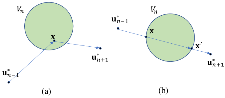
Figure 2: Two possible cases: (a) ${\bf d}\cap{\cal V}_{n}=\emptyset$; (b) ${\bf d}\cap{\cal V}_{n}\neq\emptyset$.

According to Theorem 1, the inner optimization problem can be modified as follows. For path $m$, the collection points can be optimized as follows:

$$\{{\bf u}_{m(1)}^{\ast},\ldots,{\bf u}_{m(N)}^{\ast}\}=\operatorname*{\arg\!\min}_{{\bf u}_{m}(n),\ n=1,\ldots,N}D_{m}$$ (8)

$$\mbox{subject to}\ {\bf u}_{m(n)}\in\bar{\cal V}_{m(n)},\ n=1,\ldots,N,$$ (9)

The feasible set of the inner optimization in (5) is ${\cal F}=\cup_{n}{\cal V}_{n}\subseteq{\mathbb{R}}^{2N}$, which can be replaced with ${\cal F}=\cup_{n}\bar{\cal V}_{n}\subseteq{\mathbb{R}}^{N}$ when the inner optimization in (9) is considered. This results in a decrease of computational complexity when solving the inner optimization problem, while the UAV can successfully perform data collection by crossing the boundaries of communication regions as illustrated in Example 2.

In Theorem 1, it is assumed that the communication regions of ground nodes do not overlap. However, if ground nodes are randomly deployed, there can be ground nodes that are closely located so that their communication regions can overlap as illustrated in Fig. 3. In this case, the UAV can pass the intersection of the ground nodes’ communication regions (or cross the boundary of the intersection) to collect data from all of them, because the data collection time is sufficiently short (according to Assumption of A1). As a result, we only need to consider the intersection rather than individual communication regions. A generalization of Theorem 1 is given below.

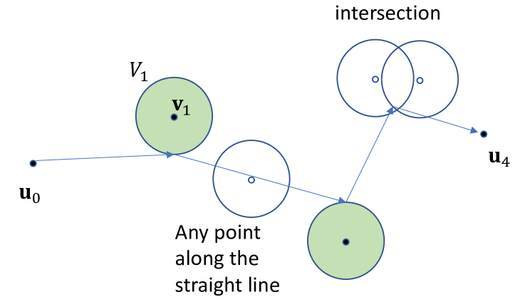
Figure 3: All the cases of communication regions.

Theorem 2

Suppose that some ${\cal V}_{n}$’s have nonempty intersection when the corresponding ground users are closely located. The intersection of those communication regions becomes the area that the UAV can collect the data of all the associated ground users, which form a cluster. If ${\cal V}_{n}$ has no intersection with other ${\cal V}_{n^{\prime}}$ , $n\neq n^{\prime}$, itself forms a cluster. Then, there are $\bar{N}\leq N$ clusters, denoted by ${\cal W}_{n}$, and the UAV needs to pass through $\bar{N}$ clusters. Then, there exists at least one optimal collection point that lies on the boundary of ${\cal W}_{n}$.

Proof:

The proof is identical to that of Theorem 1 as Lemma 1 is valid as long as the ${\cal W}_{n}$’s are convex sets. Since the intersection of closed convex sets is also a closed convex set [16], any ${\cal W}_{n}$ is a closed convex set, which completes the proof. ∎

IV-B Numerical Techniques

Based on our findings from the previous subsection, when searching for optimal solutions, it is sufficient to examine the boundaries of the feasible solution sets. In this subsection, we discuss numerical techniques to perform the inner optimization for a given order of nodes that the UAV visits. For simplicity, we do not consider (6), but two steps: i) an order of sensor nodes is found by solving the conventional TSP using any well-known algorithm (e.g., for numerical results in Subsection V-B, an open source library the Google OR-Tools is used); ii) the optimal data collection point for each sensor or intersection of sensors (that are in close proximity) is determined by solving (9).

To solve (9), we consider a finite set of $K$ points on each boundary by quantizing them. Thus, a better approximation is obtained with a larger $K$ at the cost of computational complexity. The details of the implementation are shown in the following pseudocode.

Pseudocode 1 Generating $K$ candidate points on the boundary

1:Input: $m^{\ast},v_{m(n)},r_{m(n)},\mathcal{V}_{m(n)},\mathcal{N}(\mathcal{V}_{m(n)})$

2:Output: $u_{m(n)}^{\ast}$

3:Initializations: $u_{m(n)}\leftarrow\emptyset,~{}p_{m(n)}\leftarrow\emptyset,~{}\phi_{m(n)}\leftarrow\emptyset$

4:$\mathcal{Q}(v_{1},r_{1},\theta=[\phi_{1},\phi_{2}],K)\leftarrow$ Quantize equidistant K points

5:$\mathcal{I}(v_{1},r_{1},v_{2},r_{2})\leftarrow$ Intersection points between two circles

6:$\mathcal{A}(v_{1},p_{1})\leftarrow$ Calculate radians from centre and boundary point

7:for $n=1$ to $N$ do

8:    if $\mathcal{N}(\mathcal{V}_{m(n)})=\emptyset$ then

9:        $u_{m(n)}\leftarrow$ $\mathcal{Q}(v_{m(n)},r_{m(n)},\theta=[0,2\pi],K)$

10:$\triangleright$ Between 0 and 2$\pi$ radians

11:    else

12:        for $i\in\mathcal{N}(\mathcal{V}_{m(n)})$ do

13:           $p_{m(n)}$ = $p_{m(n)}\cup\mathcal{I}(v_{m(n)},r_{m(n)},v_{m(i)},r_{m(i)})$

14:$\triangleright$ All intersecting points

15:        end for

16:        for $p\in p_{m(n)},i\in\mathcal{N}(\mathcal{V}_{m(n)})$ do

17:           if $p$ not in $\mathcal{V}_{m(i)}$ then $\triangleright$ Determine intersecting arc

18:               $p_{m(n)}=p_{m(n)}-p$

19:           end if

20:           $\phi_{m(n)}=\phi_{m(n)}\cup\mathcal{A}(p,v_{m}(n))$

21:        end for

22:        $u_{m(n)}\leftarrow$ $\mathcal{Q}(v_{m(n)},r_{m(n)}$, $\theta=[\text{min}(\phi_{m(n)})$

23:        , $\text{max}(\phi_{m(n)})],K~{}/\mid\mathcal{N}(\mathcal{V}_{m(n)})\mid)$

24:$\triangleright$ Quantize points on the intersecting arc

25:    end if

26:end for

27:$\{u_{m(1)}^{\ast},\cdots,u_{m(N)}^{\ast}\}$ = Solve$(u_{m(1)},\cdots,u_{m(N)})$ using (9)

V A Case Study: Data Collection for Smart Farming

In this section, we consider a case study with $N$ sensor nodes that are distributed over an area of operation (AO) of a river, where the AO is a rectangular area of a length of $L$ (km) and a width of $W$ (km). Each sensor node is able to capture environmental data and transmit it $M$ times a day. This data can help farmers make informed decisions. However, each node is powered by a battery and may not be able to send data directly to a remote AP or the BS in order to conserve energy and prolong the battery life. As a result, as discussed earlier, a UAV as a data mule is used to collect the data from all the nodes and upload it at the BS.

V-A Energy Consumption Model

There are two different kinds of energy consumption to take into account as follows.

V-A1 UAV

Energy consumption model for an UAV is mainly based on the amount of energy used by the UAV to travel the necessary distance for collecting data from all nodes and arriving at the BS, which is given by

$$E_{\text{uav}}=cD-c_{0},$$ (10)

where $c$ and $c_{0}$ are constants and $D$ is the travel distance of the UAV [17]. In this paper, we only consider a specific UAV, i.e., the DJI Mavic 3 [18]. The values of key parameters are given in Table I, where we can also see that the maximum energy of UAV, denoted by $E_{\text{uav}}^{\text{max}}$, is limited (due to its battery capacity).

TABLE I: Parameter settings for the UAV

Parameter	Values
Type	DJI Mavic 3 [18]
Maximum energy ($E_{\text{uav}}^{\text{max}}$)	213, 444 J(oule)
Maximum distance ($D^{\text{max}}$)	30 km
Constant velocity (V)	60 km/hr

V-A2 Sensors

The energy consumed by a sensor node with a communication range, $r$, denoted by $E_{\rm s}$, based on (3), is given by

$$E_{\rm s}=P_{\rm g}T_{\rm c}=r^{\eta}\overline{{\sf SNR}}N_{0}T_{\rm c},$$ (11)

where $\overline{{\sf SNR}}$ represents the target SNR. In Table II, we consider key parameters for a specific sensor node, where the peak transmit power of sensor, denoted by $P_{g}^{\text{max}}$, is limited.

TABLE II: Parameter settings for the UAV

Parameter	Values
Type	RN2903 [19]
Maximum transmission power ($P_{g}^{\rm max}$)	18.5 dBm
Protocol	LoRaWAN, Class A

Consequently, the overall cost function can be defined as a weighted total energy, i.e., $C(r)=\lambda E_{\rm s}+E_{\rm uav}$, where $\lambda\geq 0$ is the weighting factor that determines the relative importance of the two energy terms. Since the cost of replacing batteries at nodes can be expensive, we expect to have a large $\lambda$ (i.e., $\lambda\geq 1$).

Through Example 2, we can see that an increase in $r$ can lead to a decrease in $D$ and a decrease in $E_{\rm uav}$, but as shown in (11), increasing $r$ may result in a significant increase in $E_{\rm s}$. Thus, we aim to optimize $r$ to minimize the cost function while taking into account the constraints $E_{\text{uav}}^{max}$ for the UAV and $P_{g}^{\rm max}$ for a sensor. Note that due to a finite $P_{g}^{\rm max}$, we have $r^{\eta}\overline{{\sf SNR}}N_{0}\leq P_{g}^{\rm max}$ or $r\leq r_{s}^{\ast}$, where $r_{s}^{\ast}$ is the maximum communication range with $P_{g}^{\rm max}$ for given target SNR. In addition, the travel distance of UAV decreases with $r$. In particular, if $r=0$, the travel distance of UAV becomes maximum and the resulting $E_{\rm uav}$ can be greater than the total energy of UAV, $E_{\text{uav}}^{\text{max}}$. Thus, we have $r\geq r^{\ast}_{\rm uav}$, where $r^{\ast}_{\rm uav}$ represents the minimum communication range to satisfy $E_{\rm uav}\leq E_{\text{uav}}^{\text{max}}$. Consequently, we have the following feasible solution of $r$:

$$r^{\ast}_{\rm uav}\leq r\leq r_{s}^{\ast},$$ (12)

where $r^{\ast}_{\rm uav}\leq r_{s}^{\ast}$, and the optimal $r$ minimizing $C(r)$ subject to (12) for energy-efficient data collection by UAV can be found as

$$r^{\ast}=\operatorname*{\arg\!\min}_{r^{\ast}_{\rm uav}\leq r\leq r_{s}^{\ast}}C(r).$$ (13)

V-B Numerical Results

In this subsection, we present numerical results for the case study described in the previous subsection with the AO of $(W,L)=(20,20)$ in km.

Fig. 4 shows the consumed energy curves of the UAV and sensors when $\overline{{\sf SNR}}=6$ dB and $N=8$ as $r$ varies from 0 to 8 km. As expected, the energy consumed by the UAV decreases with $r$, while that by $N$ sensors increases with $r$. As a result, the total weighted energy curve (with $\lambda=10^{6}$) has a U-shape and an optimal communication range that minimizes the total energy consumption can be found. Note that in this result, the energy consumed by the UAV does not approach 0 although $r$ increases. Since it is assumed that the UAV will fly regardless of $r$, the minimum consumed energy of the UAV cannot be 0, but becomes the value corresponding to the shortest travel distance between ${\bf u}_{0}$ and ${\bf u}_{N+1}$.

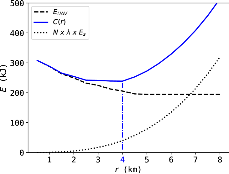
Figure 4: The energy consumed by the UAV and sensors with $\overline{{\sf SNR}}=6$ dB and $N=8$ for different values of communication ranges.

Fig. 5 shows the optimal communication range under different conditions. With $\overline{{\sf SNR}}=6$ dB, $r^{\ast}$ is shown in Fig. 5(a) for different values of $N$. As the number of sensors increases, the energy consumed by the UAV for data collection can increase. To mitigate this increase, $r^{\ast}$ can increase with $N$. In Fig. 5(b), with $N=5$, $r^{\ast}$ is found as as a function of $\overline{{\sf SNR}}$. To meet the required SNR, a shorter $r^{\ast}$ is expected when $\overline{{\sf SNR}}$ increases.

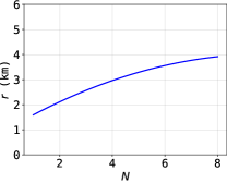
(a) $r^{\ast}$ for varying $N$

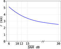
(b) $r^{\ast}$ for varying $\overline{{\sf SNR}}$

Figure 5: Optimal communication range of sensors, $r^{\ast}$: (a) $r^{\ast}$ as a function of $N$ with $\overline{{\sf SNR}}=15$ dB; (b) $r^{\ast}$ as a function of $\overline{{\sf SNR}}$ with $N=5$.

In Fig. 6, we present a comparison between the energy consumption of a conventional TSP approach and our proposed method for different numbers of sensors. The results indicate that the energy savings achieved by our method become more significant as the number of sensors increases, highlighting the efficiency of our approach, particularly for large values of $N$.

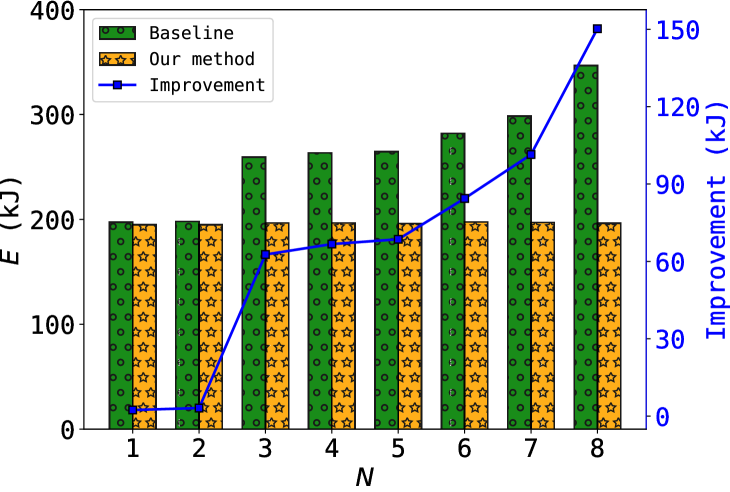
Figure 6: Comparison of energy consumption by UAV using baseline approach versus our method for varying numbers of sensor nodes

In Fig. 7, we evaluate the impact of the number of candidate points $K$ in minimizing the cost function while also analyzing the computational complexity of our method in terms of Floating Point Operations Per Second (FLOPS).

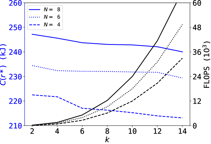
Figure 7: Minimum cost function, $C(r^{\ast})$, and computational efficiency (in FLOPS) as a function of candidate points.

VI Concluding Remarks

In this paper, we focused on collecting measurements from distributed sensors using a UAV. We rigorously demonstrated that an optimal solution for the generalized TSP can be found at a point on the boundary of each sensor’s communication region or at the intersection of communication ranges when sensors are in close proximity. Our key observation suggests that the travel distance decreases with the communication range of sensors. Using this insight, we formulated an optimization problem to minimize the weighted total consumed energy of the UAV and sensors by finding the optimal communication range.

References

- [1] M. Nemati, S. R. Pokhrel, and J. Choi, “Modelling data aided sensing with UAVs for efficient data collection,” IEEE Wireless Communications Letters, vol. 10, no. 9, pp. 1959–1963, 2021.
- [2] D.-H. Tran, V.-D. Nguyen, S. Chatzinotas, T. X. Vu, and B. Ottersten, “UAV relay-assisted emergency communications in IoT networks: Resource allocation and trajectory optimization,” IEEE Trans. Wireless Communications, vol. 21, no. 3, pp. 1621–1637, 2022.
- [3] F. Rinaldi, H.-L. Maattanen, J. Torsner, S. Pizzi, S. Andreev, A. Iera, Y. Koucheryavy, and G. Araniti, “Non-Terrestrial Networks in 5G & Beyond: A Survey,” IEEE Access, vol. 8, pp. 165178–165200, 2020.
- [4] M. Nemati, B. Al Homssi, S. Krishnan, J. Park, S. W. Loke, and J. Choi, “Non-terrestrial networks with UAVs: A projection on flying ad-hoc networks,” Drones, vol. 6, no. 11, 2022.
- [5] R. C. Shah, S. Roy, S. Jain, and W. Brunette, “Data mules: Modeling and analysis of a three-tier architecture for sparse sensor networks,” Ad Hoc Networks, vol. 1, no. 2-3, pp. 215–233, 2003.
- [6] R. Sugihara and R. K. Gupta, “Path planning of data mules in sensor networks,” ACM Trans. Sen. Netw., vol. 8, aug 2011.
- [7] S. Kim and I. Moon, “Traveling salesman problem with a drone station,” IEEE Transactions on Systems, Man, and Cybernetics: Systems, vol. 49, no. 1, pp. 42–52, 2018.
- [8] D. Bookstaber, “Simulated annealing for traveling salesman problem,” SAREPORT. nb, 1997.
- [9] N. M. Razali, J. Geraghty, et al., “Genetic algorithm performance with different selection strategies in solving TSP,” in Proceedings of the world congress on engineering, vol. 2, pp. 1–6, 2011.
- [10] E. M. Arkin and R. Hassin, “Approximation algorithms for the geometric covering salesman problem,” Discrete Applied Mathematics, vol. 55, no. 3, pp. 197–218, 1994.
- [11] M. De Berg, J. Gudmundsson, M. J. Katz, C. Levcopoulos, M. H. Overmars, and A. F. Van Der Stappen, “TSP with neighborhoods of varying size,” Journal of Algorithms, vol. 57, no. 1, pp. 22–36, 2005.
- [12] B. Yuan and T. Zhang, “Towards solving TSPN with arbitrary neighborhoods: A hybrid solution,” in Artificial Life and Computational Intelligence: 3rd Australasian Conference, pp. 204–215, Springer, 2017.
- [13] A. Nedjatia and B. Vizvárib, “Robot path planning by traveling salesman problem with circle neighborhood: Modeling, algorithm, and applications,” arXiv preprint arXiv:2003.06712, 2020.
- [14] C.-F. Cheng and C.-F. Yu, “Data gathering in wireless sensor networks: A combine–tsp–reduce approach,” IEEE Transactions on Vehicular Technology, vol. 65, no. 4, pp. 2309–2324, 2015.
- [15] A. A. Khuwaja, Y. Chen, N. Zhao, M.-S. Alouini, and P. Dobbins, “A survey of channel modeling for UAV communications,” IEEE Communications Surveys & Tutorials, vol. 20, no. 4, pp. 2804–2821, 2018.
- [16] S. Boyd and L. Vandenberghe, Convex Optimization. Cambridge University Press, 2009.
- [17] H. Yan, S.-H. Yang, Y. Ding, and Y. Chen, “Energy consumption models for UAV communications: A brief survey,” in 2022 IEEE International Conferences on Internet of Things (iThings), pp. 161–167, 2022.
- [18] D. Official, “Mavic 3 - specs - dji.” https://www.dji.com/au/mavic-3/specs. (Accessed on 04/20/2023).
- [19] Libelium, “Rn2903 - specs.” https://development.libelium.com/plug-and-sense-technical-guide/radio-modules. (Accessed on 04/20/2023).