Vanishing threshold in depolarization of correlated opinions on social networks

Abstract

The process of opinion depolarization is assumed to be mediated through social networks, where interacting individuals reciprocally exert social influence leading to a consensus. While network topology plays a decisive role in many networked dynamical processes, its effect on depolarization dynamics remains unclear. Here, we show that, in a recently proposed opinion depolarization model, the threshold of the transition from correlated and polarized opinions to consensus can vanish on heterogeneous social networks. Our theoretical findings are validated by running numerical simulations on both synthetic and real social networks, confirming that a polarized yet heterogeneously connected population can reach a consensus even in the presence of weak social influence.

The emergence of opinion polarization, which usually refers to the presence of two groups in a population holding opposite and potentially extreme opinions McCoy et al. (2018), can have a negative impact on society, providing a breeding ground for the dissemination of harmful misinformation Vicario et al. (2019). Consequently, researchers from distinct scientific disciplines have embarked on studying different mechanisms that could potentially reduce opinion polarization, a process referred to as depolarization in the literature Vinokur and Burnstein (1978); Miller et al. (1993). Given the limited availability of reliable data on opinions spanning an extended period, most studies have concentrated on a theoretical understanding of opinion depolarization Matakos et al. (2017); Musco et al. (2018); Balietti et al. (2021).

Several modeling efforts have explored various mechanisms underlying the opinion formation process, such as homophily Axelrod (1997); Baumann et al. (2020), bounded confidence Deffuant et al. (2000); Hegselmann and Krause (2002), or opinion rejection Martins et al. (2010); Crawford et al. (2013). While earlier studies typically focused on a single topic Sznajd-Weron and Sznajd (2000); López-Pintado and Watts (2008), researchers recently have proposed novel modeling frameworks to address the case of multi-dimensional opinions Parsegov et al. (2017); Schweighofer et al. (2020); Chen et al. (2021), where opinions can vary across different topics. Notably, when multiple topics are considered, correlations between opinions may arise Baldassarri and Gelman (2008); Benoit and Laver (2012); DellaPosta et al. (2015); Falck et al. (2020). For instance, racism and the stereotype of blacks as violent individuals may be related to gun ownership and opposition to gun control policies in US whites O’Brien et al. (2013).

One possibility to meaningfully study opinion dynamics regarding two interdependent topics is to represent them in the polar plane Ojer et al. (2023), where the angle $\varphi$ represents the orientation of an individual with respect to both topics and the radius $\rho$ expresses his/her attitude strength or conviction. Such a polar representation allows for a natural interpretation of opinion polarization, typically represented by groups with opposite orientations $\varphi$ in the polar plane (regardless of the conviction value $\rho$) Esteban and Ray (1994). In particular, two individuals holding contrary opinions with respect to two topics will be represented by opposite orientations, maximally separated by an angle $\pi$. On the other hand, consensus, representing individuals converging towards a common ground Degroot (1974), is reached when agents align their orientation to a common value. The angular distribution $P(\varphi)$ permits to easily identify correlations between opinions: when opinions are polarized and strongly correlated, $P(\varphi)$ is characterized by two peaks (bimodal distribution), corresponding to the opposite ideologies at play. For instance, political ideology could be defined by two major axes, the economic axis (left vs right) measuring the desire for state intervention in the economy, and the social axis (libertarian vs authoritarian) measuring the desire for personal freedom . Within this context, the polar representation intuitively shows that a population characterized by two groups with opposite orientations (such as left and libertarian vs right and authoritarian) is more polarized than two groups with a smaller distance, measured by the orientation difference (left vs right, both libertarian).

The process of opinion depolarization can be represented as a phase transition from an initially polarized opinion state to a consensus, typically due to the social influence exerted by individuals on their peers Currin et al. (2022); Pal et al. (2023); Sobkowicz (2023). When multiple topics are taken into account, the correlations between opinions may play an important role Baumann et al. (2021), triggering in some cases an explosive depolarization transition Ojer et al. (2023). Understanding the nature of such a transition, determined by the modeling framework, is crucial to determine under which conditions the population is able to reduce opinion polarization more effectively. These conditions may include the connectivity of the social network underlying the process of opinion formation, which is generally assumed to be mediated by social interactions. While the network topology has been shown to play a pivotal role in different networked dynamical processes Barrat et al. (2008), its effect in depolarization models has not been explored yet.

In this paper, we address this important open question by analytically studying a recently proposed opinion depolarization model, the so-called social compass model, in which two interdependent topics are represented in the polar plane Ojer et al. (2023). We assume polarized and strongly correlated initial opinions, as is reported through different experiments like empirical opinion surveys regarding controversial topics Miller et al. (1993); DiMaggio et al. (1996); Ojer et al. (2023). We then contrast two different theoretical approaches to investigate the conditions for the emergence of consensus. We show that, when a non-trivial connectivity is assumed among the interacting agents, the depolarization threshold is entirely determined by the network topology. For heterogeneous (thus realistic) social networks, we demonstrate a vanishing threshold for the social influence needed to trigger the depolarization of the population. Our theoretical findings are validated by running extensive simulations of the depolarization model on both synthetic and empirical social networks, confirming that the initial polarized state is very susceptible to disappear even when social influence among individuals is very weak.

The social compass model. Let us consider a set of $N$ agents, each one endowed with a conviction, $\rho_{i}$, and a preferred orientation, $\varphi_{i}$. The evolution of the orientation in time, $\theta_{i}(t)$, is determined by two competing factors: individuals are i) subject to the social influence of their peers and ii) stubborn to their initial, preferred orientation $\theta_{i}(0)=\varphi_{i}$. This dynamics can be modeled by the set of ordinary differential equations Ojer et al. (2023)

$$\dot{\theta}_{i}(t)=\rho_{i}\sin\left[\varphi_{i}-\theta_{i}(t)\right]+\lambda\sum_{j=1}^{N}a_{ij}\sin\left[\theta_{j}(t)-\theta_{i}(t)\right].$$ (1)

The first term in Eq. (1) models the tendency of individuals to remain close to their preferred orientation, which we assume to be proportional to their conviction, considered constant in time. The second term accounts for the social influence of peers, mediated by a social network Jackson (2010) with adjacency matrix $a_{ij}$ Newman (2010), taking the value $a_{ij}=1$ when agents $i$ and $j$ are socially connected and $a_{ij}=0$ otherwise. The social influence, quantified by the coupling constant $\lambda$, tends to make the orientation of an agent aligned to the orientation of their neighbors. Figure 1 illustrates the basic mechanisms of the social compass model.

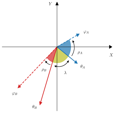
Figure 1: Illustrative scheme of the social compass model. We sketch two connected individuals, $A$ and $B$, holding conviction $\rho_{A}$ and $\rho_{B}$, and initial orientation $\varphi_{A}$ and $\varphi_{B}$, respectively, towards two distinct topics $X$ and $Y$. Their orientations $\theta_{A}$ and $\theta_{B}$ evolve in time as the result of two competing forces: they tend to align with their initial orientation proportionally to their conviction, and they are subject to reciprocal social influence proportionally to the coupling strength $\lambda$.

The model is completely defined by the probability distributions $P(\rho)$ and $P(\varphi)$ that a randomly chosen agent has conviction $\rho$ and initial orientation $\varphi$, respectively, which we assume to be statistically independent. Here, we focus on a power-law form of the conviction distribution, defined in the interval $\left[0,1\right]$,

$$P(\rho)=(\alpha+1)\rho^{\alpha},$$ (2)

with $\alpha\geq 0$, and a bimodal distribution of initial orientations,

$$P(\varphi)=\frac{1}{2}\left[\delta(\varphi)+\delta(\varphi+\pi)\right],$$ (3)

aimed at describing maximally correlated initial opinions.

In the absence of social interactions ($\lambda=0$), Eq. (1) leads to the steady state $\theta_{i}=\varphi_{i}$, i.e., every agent is aligned with their preferred orientation, which is assumed to be a polarized state. For large $\lambda$, on the other hand, social influence prevails over stubbornness and a depolarized (consensus) state emerges, with all the agents having the same average orientation $\theta_{i}\simeq\psi$. Therefore, the model exhibits a phase transition from a polarized to a consensus phase. At the mean-field level, where each individual interacts socially with every other, this transition occurs at the threshold value of the coupling constant Ojer et al. (2023)

$$\lambda_{c}^{\mathrm{MF}}\left(\alpha\right)=\frac{\alpha}{\alpha+1}.$$ (4)

In the following, we will show that, when social influence among individuals is mediated by a general social network, the threshold value of the depolarization transition can vanish, contrary to the mean-field case. We compare two different approaches: the heterogeneous mean-field (HMF) approximation Pastor-Satorras and Vespignani (2001) and the perturbation theory Restrepo et al. (2005).

Heterogeneous mean-field approximation. For uncorrelated networks Newman (2002), the HMF approximation is equivalent to the so-called annealed network approximation Dorogovtsev et al. (2008), in which the adjacency matrix can be replaced by its annealed form $a_{ij}\simeq\frac{k_{i}k_{j}}{N\langle k\rangle}$ Boguñá et al. (2009). Within this approximation, one can characterize the depolarization transition in terms of a degree averaged complex global order parameter Ichinomiya (2004)

$$r(\lambda)\mathrm{e}^{i\psi}=\frac{1}{N\langle k\rangle}\sum_{j=1}^{N}k_{j}\mathrm{e}^{i\theta_{j}(\lambda)},$$ (5)

where $\theta_{j}(\lambda)$ is computed at the steady state and $\langle...\rangle$ denotes the average value. $r(\lambda)$ represents the degree of consensus among the population, with $r\simeq 0$ at the polarized state and $r\simeq 1$ at the consensus state, while $\psi$ measures the average opinion orientation at consensus. The threshold condition for the emergence of a depolarized phase can then be obtained by inserting Eq. (3) into Eq. (1) and considering the instability of the solution $r=0$ in the self-consistent equation ensuing in the steady state. This leads to the HMF threshold (see Supplemental Material, Sec. I (SM I))

$$\lambda_{c}^{\mathrm{HMF}}=\frac{\langle k\rangle}{\langle k^{2}\rangle}\lambda_{c}^{\mathrm{MF}},$$ (6)

where $\lambda_{c}^{\mathrm{MF}}$ corresponds to the mean-field threshold Eq. (13).

This result, recovered also in epidemic spreading Boguñá and Pastor-Satorras (2002); Boguñá et al. (2003) and synchronization phenomena Ichinomiya (2004); Lee (2005), indicates that, if the degree fluctuations are very large, the threshold can become negligibly small. In the particular case of scale-free networks Barabási and Albert (1999), with a power-law degree distribution $P(k)\sim k^{-\gamma}$, for $\gamma\leq 3$ the second moment $\langle k^{2}\rangle$ diverges for an infinitely large network and therefore $\lambda_{c}^{\mathrm{HMF}}$ tends to zero. In the present modeling framework, this result implies that, if the underlying social network is characterized by such realistic topology, any non-zero value of social influence can lead the system from polarization to consensus. Thereby, afar from the thermodynamic limit $N\to\infty$, the more heterogeneous the underlying social network, the smaller the expected threshold for the depolarization of the system. On the other hand, for $\gamma>3$ we obtain that $\langle k^{2}\rangle$ converges to a constant and therefore $\lambda_{c}^{\mathrm{HMF}}>0$. Thus, a nonzero threshold is obtained for weakly heterogeneous networks, even in the thermodynamic limit.

It is worth stressing that the depolarization threshold can vanish only if interactions are mediated by an (infinitely large) broad-tailed social network, while the threshold is finite for other network topologies and in particular in the mean-field case, when all individuals are connected all-to-all. The only exception to this general behavior holds for a uniform conviction distribution ($P(\rho)$ with exponent $\alpha=0$), where according to Eq. (13), $\lambda_{c}^{\mathrm{MF}}(\alpha=0)=0$. Indeed, at the mean-field level, the order parameter behaves for $\lambda\to 0$ as (see SM IA)

$$r\sim\frac{2}{\lambda}\mathrm{e}^{-1/\lambda}.$$ (7)

In this special case of $\alpha=0$ one can show that, for any degree distribution $P(k)$, a zero threshold is also recovered, indicating that a uniform conviction is a sufficient condition to obtain a vanishing threshold for any network structure; see SM IA.

Perturbation theory. Beyond the HMF approximation, one can tackle the general equation Eq. (1) relying on the spectral properties of the adjacency matrix of the social network, a method that has been proved to provide a better description of some dynamical processes on networks, such as the susceptible-infected-susceptible model of epidemic spreading Castellano and Pastor-Satorras (2010); Ferreira et al. (2012). An analytical treatment of the model starts from the complex local order parameter Restrepo et al. (2005)

$$r_{j}\mathrm{e}^{i\psi_{j}}=\sum_{\ell=1}^{N}a_{j\ell}\mathrm{e}^{i\theta_{\ell}(\lambda)},$$ (8)

with $r_{j}$ being a local measure of order and $\psi_{j}$ the local average orientation, computed over the nearest neighbors of an agent. Similarly to the HMF approximation, the depolarized phase is characterized by the local consensus among the agents, i.e., $r_{j}>0$. Solving for the steady state, we can then determine the threshold value of the coupling constant by letting $r_{j}\to 0$, which leads to (see SM II)

$$\lambda_{c}^{\mathrm{P}}=\frac{\lambda_{c}^{\mathrm{MF}}}{\Lambda_{m}},$$ (9)

where $\Lambda_{m}$ is the largest eigenvalue of the adjacency matrix. In the case of uncorrelated scale-free networks with a maximum degree $k_{c}$, this largest eigenvalue can be estimated as  Chung et al. (2003); Castellano and Pastor-Satorras (2010)

$$\Lambda_{m}\simeq\begin{cases}\langle k^{2}\rangle/\langle k\rangle&2<\gamma<5/2\\ \sqrt{k_{c}}&\gamma>5/2\end{cases}.$$ (10)

Since $k_{c}$ grows as a function of $N$ for any $\gamma$ Boguñá et al. (2009, 2004), the consequence of Eq. (10) is remarkable: in any uncorrelated random network with power-law distributed connectivities, the threshold value goes to zero as the network size goes to infinity. This is in contrast with the HMF approximation given by Eq. (11), since a constant threshold is not observed for $\gamma>3$.

In order to check the previous theoretical analysis, in the following we test the different predictions of both HMF approximation and perturbation theory, $\lambda_{c}^{\mathrm{HMF}}$ and $\lambda_{c}^{\mathrm{P}}$ respectively, on synthetic and empirical networks; see SM IIIA for simulation details.

Synthetic networks. We build uncorrelated scale-free synthetic networks using the uncorrelated configuration model (UCM) Catanzaro et al. (2005) with a minimum degree $k_{\mathrm{min}}=3$ and maximum degree $k_{c}=\mathrm{min}\left(N^{1/2},N^{1/(\gamma-1)}\right)$ Boguñá et al. (2009, 2004). We consider degree exponents $\gamma=2.5$ and $\gamma=3.5$ to distinguish the two regimes (vanishing and non-vanishing threshold) of the HMF approximation. For simplicity, we study the case $\alpha\to\infty$, i.e., $\rho_{i}=1$ $\forall i$, which leads to $\lambda_{c}^{\mathrm{MF}}=1$.

In Figure 2 (a) we tested the finite-size scaling of the depolarization threshold estimated by numerical simulations of the social compass model on scale-free UCM networks, by plotting it as a function of network size $N$. As we can see, the threshold $\lambda_{c}$ decreases continuously for increasing $N$, for all values of $\gamma$. The theoretical HMF prediction, Eq. (11), depicted as a dashed line, works quite well for $\gamma=2.5$. However, it predicts a constant threshold for $\gamma>3$ in the thermodynamic limit, which is not compatible with numerical results for $\gamma=3.5$.

Instead, numerical simulations are compatible with the perturbation theory and with a vanishing threshold for large $N$ and for any $\gamma$. Indeed, in Figure 2 (b) we show the inverse of the depolarization threshold $1/\lambda_{c}$ as a function of the largest eigenvalue $\Lambda_{m}$, with the theoretical prediction of the perturbation theory, Eq. (9), depicted as a black dashed line. As we can see, the numerical results are recovered with good accuracy by the theoretical expression, which predicts the correct scaling of the numerical threshold up to a constant multiplicative factor. We notice, however, that the agreement between theory and simulations is better for $\gamma=2.5$ than for $\gamma=3.5$, in which the perturbation theory prediction is recovered for the largest values of $\Lambda_{m}$, corresponding to large network sizes. Thus, we can attribute the deviation of the case $\gamma=3.5$ from the theory to finite-size effects.

One could argue that the validity of the perturbation theory is contingent to the assumption of a local order parameter, Eq. (19), being close to zero in the vicinity of the polarized state. The vanishing of the local order parameter can only be achieved when it is computed over a sufficiently large number of nearest neighbors. Thus, one might expect that perturbation theory would work better for networks with larger connectivity, i.e., with a larger average degree. The average degree grows in UCM networks with decreasing $\gamma$, so we could expect that perturbation theory prediction is more accurate for smaller values of $\gamma$. We checked that this intuition is not correct by performing numerical simulations on UCM networks with $\gamma=3.5$ and a larger average degree, obtained by imposing $k_{\mathrm{min}}=10$. The results (not shown) indicate that the performance of the perturbation theory is not increased by a larger average degree. We conclude then that perturbation theory is valid in general for scale-free networks with any exponent $\gamma$ in the thermodynamic limit, corresponding to large network size and large largest eigenvalue.

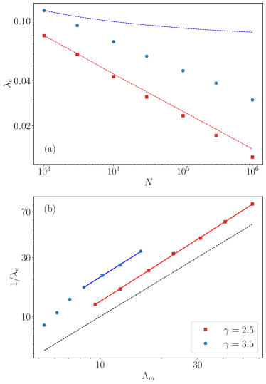
Figure 2: Depolarization threshold on synthetic networks. (a) Numerical threshold $\lambda_{c}$ as a function of $N$ for scale-free synthetic networks with different exponents $\gamma$. The dashed lines, representing the theoretical prediction of the HMF theory, have been arbitrarily shifted to ease comparison with numerical data. (b) Inverse of the numerical threshold $1/\lambda_{c}$ as a function of $\Lambda_{m}$ for different values of $\gamma$. The dashed line represents the theoretical prediction of the perturbation theory. Solid lines represent power regression $1/\lambda_{c}\sim\Lambda_{m}^{a}$, with $a=1.05\pm 0.01$ for $\gamma=2.5$ and $a=1.04\pm 0.02$ for $\gamma=3.5$. Due to finite-size effects, the power regression for $\gamma=3.5$ is performed over the four largest network sizes. Initial opinions: constant conviction $\rho=1$, given by Eq. (2) for $\alpha\to\infty$, and bimodal orientation, given by Eq. (3). Each point is averaged over 100 UCM network realizations, being the eigenvalue of the adjacency matrix computed as the mean value of all the realizations. Error bars are smaller than symbols.

Empirical networks. To check the validity of our theoretical prediction in a more general scenario than the synthetic UCM model, we performed simulations of the social compass model on a set of 25 real social networks representing user-user interactions in online networking platforms, such as direct messages or friendship connections. Networks range in sizes between $N=10^{3}$ and $N=3\times 10^{6}$ and have different levels of degree heterogeneity; see SM IIIB for details. In the simulations, we consider again the case of a constant conviction ($\alpha\to\infty$), so that $\lambda_{c}^{\mathrm{MF}}=1$. In Figure 3 we present a scatter plot of the inverse of the numerically estimated thresholds $1/\lambda_{c}$ as a function of the largest eigenvalue $\Lambda_{m}$ computed for each network. As we can see, the perturbation theory provides an excellent prediction of the threshold value for all the different empirical networks considered, confirming the linear scaling, Eq. (9), depicted as a black dashed line.

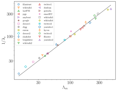
Figure 3: Depolarization threshold on empirical social networks. Inverse of the numerical threshold $1/\lambda_{c}$ as a function of $\Lambda_{m}$ for different empirical social networks. The dashed line represents the theoretical prediction of the perturbation theory. Initial opinions: constant conviction $\rho=1$, given by Eq. (2) with $\alpha=\infty$, and bimodal orientation, given by Eq. (3). Each point is averaged over 10 initial orientation distributions. Error bars are smaller than symbols.

Discussion. Here we showed that the depolarization threshold of the social compass model, within a population characterized by heterogeneous social interactions, can be very small. This indicates that even a weak social influence among individuals may be able to trigger consensus. This result is particularly relevant since most empirical social networks are highly heterogeneous, so it could be easier to reduce opinion polarization in these realistic settings. A smaller depolarization threshold for increasingly heterogeneous social networks can be understood by the presence of highly connected nodes (hubs) extending their social influence to a large number of nodes, while the social influence they receive from those neighbors is averaged down. Therefore, the presence of hubs promotes the formation of consensus, decreasing the depolarization threshold.

It is important to discuss if these findings can generalize beyond the specific case of the social compass model. To this aim, we considered different definitions of the model by replacing the sine in the first term of Eq. (1) (describing the tendency of individuals to remain close to their preferred orientation) with similar functions. One should consider odd functions in order to preserve the correct representation of the orientations in the polar plane. Furthermore, one needs monotonic functions leading to a higher response if the orientation difference is greater. Finally, it is essential to ensure finite outputs from the function to avoid diverging results. These requirements describe a potential well for the orientation $\theta$ centered around the preferred orientation $\varphi$. We tested the behavior of the model by using functions respecting these requirements, such as the hyperbolic tangent $\tanh\left(\varphi_{i}-\theta_{i}\right)$ or even the simple difference $\varphi_{i}-\theta_{i}$, finding identical results, i.e., a vanishing threshold in the thermodynamic limit.

A different case holds for the second term in Eq. (1), modeling social influence among individuals. In order to capture the nature of the polar coordinates representing the opinions on two topics, the interaction term must be periodic on the angular difference $\theta_{j}-\theta_{i}$ for both angles $\theta_{j}$ and $\theta_{i}$. In terms of a harmonic decomposition Kuramoto (1975); Strogatz (2000), it is clear that the sinusoidal form chosen in both the Kuramoto model Kuramoto (1975) and the social compass model is the simplest one fulfilling the periodicity condition. Other non-periodic functions are not allowed, since they do not lead to a phase transition between two well-differentiated regimes.

However, note that despite the coupling term being the same in both models, each model’s behavior on scale-free networks is notably different from the other in the thermodynamic limit. Indeed, the depolarization threshold of the social compass model vanishes regardless of the degree heterogeneity, following the predictions of perturbation theory, Eq. (9), while the synchronization threshold of the Kuramoto model remains constant for $\gamma>3$ Peron et al. (2019), as it is predicted by a HMF theory analogous to Eq. (11). This is due to the different nature of the variables considered: while in the Kuramoto model the variables $\theta_{i}$, which represent the phases of local oscillators, become locked and rotate in synchrony for sufficiently large interactions, in the social compass model $\theta_{i}$, which represent an orientation, reach a steady, constant state at large times.

Vanishing threshold in depolarization of correlated opinions on social networks 
 
Supplemental Material

Jaume Ojer

Michele Starnini

Romualdo Pastor-Satorras

Supplemental Material

I Heterogeneous mean-field approximation

The heterogeneous mean-field (HMF) approximation consists in disregarding the actual structure of the network and keeping only a statistical description based on the degree distribution $P(k)$ Pastor-Satorras and Vespignani (2001), giving the probability that a randomly chosen agent has degree $k$ (is connected to $k$ other agents), and the conditional probability $P(k^{\prime}|k)$ that a random connection from an agent of degree $k$ points to an agent of degree $k^{\prime}$ Pastor-Satorras et al. (2001). In the simplest case of uncorrelated networks Newman (2002), where the conditional probability can be written as $P_{\mathrm{un}}(k^{\prime}|k)=k^{\prime}P(k^{\prime})/\langle k\rangle$ Pastor-Satorras et al. (2001); Dorogovtsev et al. (2008), the HMF approximation is equivalent to the so-called annealed network approximation Dorogovtsev et al. (2008), in which the adjacency matrix can be replaced by its annealed form Boguñá et al. (2009)

$$a_{ij}\simeq\bar{a}_{ij}=\frac{k_{i}k_{j}}{N\langle k\rangle}.$$ (1)

Inserting this expression into the general model equation, Eq. (1) of the main text, we obtain

$$\dot{\theta}_{i}(t)=\rho_{i}\sin\left[\varphi_{i}-\theta_{i}(t)\right]+\frac{\lambda k_{i}}{N\langle k\rangle}\sum_{j=1}^{N}k_{j}\sin\left[\theta_{j}(t)-\theta_{i}(t)\right].$$ (2)

We can introduce now the degree averaged complex global order parameter Ichinomiya (2004)

$$r(\lambda)\mathrm{e}^{i\psi}=\frac{1}{N\langle k\rangle}\sum_{j=1}^{N}k_{j}\mathrm{e}^{i\theta_{j}(\lambda)},$$ (3)

where the mean-field values $r$ and $\psi$ represent the degree of consensus among the population and the average orientation of the agents, respectively. Considering that Ichinomiya (2004)

$$\mathrm{Im}\left\{{r\mathrm{e}^{i\left(\psi-\theta_{j}\right)}}\right\}=r\sin(\psi-\theta_{j})=\mathrm{Im}\left\{{\frac{1}{N\langle k\rangle}\sum_{\ell}k_{\ell}\mathrm{e}^{i(\theta_{l}-\theta_{j})}}\right\}=\frac{1}{N\langle k\rangle}\sum_{\ell}k_{\ell}\sin(\theta_{l}-\theta_{j}),$$ (4)

we can write Eq. (2) as

$$\dot{\theta}_{i}=\rho_{i}\sin(\varphi_{i}-\theta_{i})+\lambda k_{i}r\sin(\psi-\theta_{i}),$$ (5)

in which the (apparently independent) orientation variables are coupled by means of the mean-field quantities $r$ and $\psi$. Solving the previous equation for the steady state, we can write the orientation of each agent as a function of $r$ and $\psi$, namely Ojer et al. (2023)

$$\theta_{i}(r,\psi)=\arctan\left(\frac{\lambda k_{i}r\sin(\psi)+\rho_{i}\sin(\varphi_{i})}{\lambda k_{i}r\cos(\psi)+\rho_{i}\cos(\varphi_{i})}\right).$$ (6)

Inserting this expression into the degree averaged complex global order parameter Eq. (3), averaging over the distributions $P(\rho)$ and $P(\varphi)$ and taking the continuous degree approximation, we can write Ojer et al. (2023); Ichinomiya (2004)

$$r = \frac{1}{\langle k\rangle}\int\;dkkP(k)\int\;d\rho P(\rho)\int\;d\varphi P(\varphi)\mathrm{e}^{i\left[\theta(r,\psi)-\psi\right]}$$ (7)

$$= \frac{1}{\langle k\rangle}\int\;dk\int\;d\rho\int\;d\varphi\frac{kP(k)P(\rho)P(\varphi)\left[\lambda kr+\rho\mathrm{e}^{i(\varphi-\psi)}\right]}{\sqrt{(\lambda kr)^{2}+2\lambda kr\rho\cos(\varphi-\psi)+\rho^{2}}}\equiv I_{\mathrm{HMF}}(\lambda,r,\psi).$$

Taking the real and imaginary parts of this expression, we find the relations

$$r = \mathrm{Re}\left\{{I_{\mathrm{HMF}}(\lambda,r,\psi)}\right\}\equiv I_{r}(\lambda,r,\psi),$$ (8)

$$0 = \mathrm{Im}\left\{{I_{\mathrm{HMF}}(\lambda,r,\psi)}\right\}\equiv I_{\psi}(\lambda,r,\psi).$$ (9)

The first equation defines the order parameter $r$ self-consistently, while the second relation allows us to compute the value of the average orientation $\psi$.

We can estimate the value of the threshold by looking at the condition for the onset of instability of the solution $r=0$, namely

$$\left.\frac{\partial I_{r}(\lambda,r,\psi)}{\partial r}\right|_{r=0} = \frac{1}{\langle k\rangle}\int\;dkkP(k)\int\;d\rho P(\rho)\int\;d\varphi P(\varphi)\frac{\lambda k}{\rho}\sin^{2}(\varphi-\psi)\geq 1.$$ (10)

This condition translates into the threshold

$$\lambda_{c}^{\mathrm{HMF}}=\frac{\langle k\rangle}{\langle k^{2}\rangle}\lambda_{c}^{\mathrm{MF}},$$ (11)

where

$$\lambda_{c}^{\mathrm{MF}}=\frac{1}{\int_{0}^{\infty}\;d\rho\frac{P(\rho)}{\rho}\int_{-\pi}^{\pi}\;d\varphi P(\varphi)\sin^{2}(\varphi-\psi)}$$ (12)

is the depolarization threshold at the mean-field level Ojer et al. (2023).

I.1 Threshold zero for a uniform conviction

At the mean-field level, for a power-law-distributed conviction $P(\rho)\sim\rho^{\alpha}$ and a bimodal $P(\varphi)$, Eqs. (2) and (3) of the main text respectively, the depolarization threshold Eq. (12) takes the form Ojer et al. (2023)

$$\lambda_{c}^{\mathrm{MF}}\left(\alpha\right)=\frac{\alpha}{\alpha+1},$$ (13)

which vanishes for a uniform conviction distribution with exponent $\alpha=0$. Indeed, in the case of agents connected all-to-all, the self-consistent equation for the order parameter Eq. (8) reads

$$r=\int_{0}^{1}\;d\rho\frac{\lambda r}{\sqrt{(\lambda r)^{2}+\rho^{2}}}=\lambda r\operatorname{arctanh}{\left(\frac{1}{\sqrt{(\lambda r)^{2}+1}}\right)}.$$ (14)

Apart from the solution $r=0$, corresponding to the polarized state, we find the non-zero solution

$$r(\lambda)=\frac{1}{\lambda\sinh{\left(\frac{1}{\lambda}\right)}},$$ (15)

which vanishes only for $\lambda=0$, indicating a null threshold. The asymptotic behaviors of the order parameter are then

$$r\left(\lambda\right)\sim\begin{cases}\frac{2}{\lambda}\mathrm{e}^{-1/\lambda}&\lambda\to 0\\ \frac{1}{1+\frac{1}{6\lambda^{2}}}&\lambda\to\infty\end{cases}.$$ (16)

Interestingly, the special case of a uniform conviction distribution leads to a self-consistent equation Eq. (8) for a degree distribution $P(k)$ that follows as

$$r=\frac{1}{\langle k\rangle}\int k^{2}P(k)\lambda r\operatorname{arctanh}{\left(\frac{1}{\sqrt{(\lambda kr)^{2}+1}}\right)}\;dk\equiv f(r).$$ (17)

While the integral cannot be performed in the general case, we can obtain the threshold as the value of $\lambda$ above which a non-zero solution exists. Using standard geometric arguments, we can see that a non-zero solution exists when the right-hand side of Eq. (17) fulfills the condition $\left.f^{\prime}(r)\right|_{r=0}\geq 1$. We have

$$f^{\prime}(r)=\frac{1}{\langle k\rangle}\int k^{2}P(k)\lambda\left[\operatorname{arctanh}{\left(\frac{1}{\sqrt{(\lambda kr)^{2}+1}}\right)}-\frac{1}{(\lambda kr)^{2}+1}\right]\;dk.$$ (18)

In the limit $r\to 0$, the argument of the $\operatorname{arctanh}$ tends to $1$ and this function thus diverges. Therefore, $\lim_{r\to 0}f^{\prime}(r)=\infty$ for any network structure, implying that $\left.f^{\prime}(r)\right|_{r=0}$ is larger than $1$ for any value of $\lambda$, which indicates that $\lambda_{c}^{\mathrm{HMF}}=0$.

II Perturbation theory

For social interactions mediated by a general network, an analytical treatment of the model starts from the complex local order parameter Restrepo et al. (2005)

$$r_{j}\mathrm{e}^{i\psi_{j}}=\sum_{\ell=1}^{N}a_{j\ell}\mathrm{e}^{i\theta_{\ell}(\lambda)},$$ (19)

with $r_{j}$ being a local measure of order and $\psi_{j}$ the local average orientation, computed over the nearest neighbors of an agent. Defining now $\Delta\theta_{i}\equiv\theta_{i}-\psi_{i}$ and $\Delta\varphi_{i}\equiv\varphi_{i}-\psi_{i}$, we can write the previous equation as

$$r_{j}=\sum_{\ell=1}^{N}a_{j\ell}\mathrm{e}^{i\Delta\theta_{\ell}}\mathrm{e}^{i\left(\psi_{\ell}-\psi_{j}\right)}.$$ (20)

Similarly to Eq. (5), the general model equation can be coupled as

$$\Delta\dot{\theta}_{i}=\rho_{i}\sin(\Delta\varphi_{i}-\Delta\theta_{i})-\lambda r_{i}\sin(\Delta\theta_{i}).$$ (21)

The steady state is then given by

$$\Delta\theta_{i}=\arctan{\left(\frac{\rho_{i}\sin{\left(\Delta\varphi_{i}\right)}}{\lambda r_{i}+\rho_{i}\cos{\left(\Delta\varphi_{i}\right)}}\right)}.$$ (22)

Inserting this expression into Eq. (20), we obtain Restrepo et al. (2005)

$$r_{i} = \sum_{\rho_{j}}\sum_{\varphi_{j}}\frac{a_{ij}\cos{\left(\psi_{j}-\psi_{i}\right)}\left[\lambda r_{j}+\rho_{j}\cos{\left(\Delta\varphi_{j}\right)}\right]}{\sqrt{(\lambda r_{j})^{2}+2\lambda r_{j}\rho_{j}\cos\left(\Delta\varphi_{j}\right)+\rho^{2}}}-\sum_{\rho_{j}}\sum_{\varphi_{j}}\frac{a_{ij}\sin{\left(\psi_{j}-\psi_{i}\right)}\rho_{j}\sin{\left(\Delta\varphi_{j}\right)}}{\sqrt{(\lambda r_{j})^{2}+2\lambda r_{j}\rho_{j}\cos\left(\Delta\varphi_{j}\right)+\rho^{2}}},$$ (23)

$$0 = \sum_{\rho_{j}}\sum_{\varphi_{j}}\frac{a_{ij}\sin{\left(\psi_{j}-\psi_{i}\right)}\left[\lambda r_{j}+\rho_{j}\cos{\left(\Delta\varphi_{j}\right)}\right]}{\sqrt{(\lambda r_{j})^{2}+2\lambda r_{j}\rho_{j}\cos\left(\Delta\varphi_{j}\right)+\rho^{2}}}+\sum_{\rho_{j}}\sum_{\varphi_{j}}\frac{a_{ij}\cos{\left(\psi_{j}-\psi_{i}\right)}\rho_{j}\sin{\left(\Delta\varphi_{j}\right)}}{\sqrt{(\lambda r_{j})^{2}+2\lambda r_{j}\rho_{j}\cos\left(\Delta\varphi_{j}\right)+\rho^{2}}},$$ (24)

for the real and imaginary parts, respectively. For a bimodal $P(\varphi)$, Eq. (3) of the main text, one half of the population holds $\varphi_{i}=0$ (state 1), whereas the other half $\varphi_{i}=\pi$ (state 2). Near the transition to consensus, if the number of connections per agent is large, one half of the neighbors will likely be at state 1 ($\theta_{j}=0$) and the other half at state 2 ($\theta_{j}=\pi$). Therefore, $\psi_{i}=\pi/2$ $\forall i$ such that $\psi_{j}-\psi_{i}=0$. Eqs. (23) and (24) are then reduced to

$$r_{i} = \sum_{\rho_{j}}\sum_{\varphi_{j}}\frac{a_{ij}\left[\lambda r_{j}+\rho_{j}\cos{\left(\Delta\varphi_{j}\right)}\right]}{\sqrt{(\lambda r_{j})^{2}+2\lambda r_{j}\rho_{j}\cos\left(\Delta\varphi_{j}\right)+\rho^{2}}},$$ (25)

$$0 = \sum_{\rho_{j}}\sum_{\varphi_{j}}\frac{a_{ij}\rho_{j}\sin{\left(\Delta\varphi_{j}\right)}}{\sqrt{(\lambda r_{j})^{2}+2\lambda r_{j}\rho_{j}\cos\left(\Delta\varphi_{j}\right)+\rho^{2}}},$$ (26)

respectively. Moreover, for the neighbors at state 1 $\Delta\varphi_{j}=-\pi/2$, whereas for the ones at state 2 $\Delta\varphi_{j}=\pi/2$. Hence, Eq. (26) for the imaginary part is satisfied. For the real part, approximating the sum of conviction as an integral and summing over all the agents, we obtain

$$r_{i}=\sum_{j=1}^{N}a_{ij}\int d\rho P(\rho)\frac{\lambda r_{j}}{\sqrt{(\lambda r_{j})^{2}+\rho^{2}}}.$$ (27)

We can determine the threshold value of $\lambda$ by letting $r_{i}\to 0$. Expanding the right-hand side of the previous equation at first-order, we obtain

$$r_{i}^{(0)}=\frac{\lambda}{\lambda_{c}^{\mathrm{MF}}}\sum_{j=1}^{N}a_{ij}r_{j}^{(0)},$$ (28)

where, for a power-law-distributed conviction, Eq. (2) of the main text, $\lambda_{c}^{\mathrm{MF}}$ is the threshold value Eq. (13) at the mean-field level. We thus identify the depolarization threshold of the coupling constant with the largest eigenvalue $\Lambda_{m}$ of the adjacency matrix Restrepo et al. (2005), obtaining

$$\lambda_{c}^{\mathrm{P}}=\frac{\lambda_{c}^{\mathrm{MF}}}{\Lambda_{m}}.$$ (29)

III Numerical results

In order to verify the validity of our theoretical predictions, we performed extensive numerical simulations of the model on both synthetic and empirical social networks.

III.1 Simulation details

Simulations are performed by numerically integrating the general model equation, Eq. (1) of the main text, starting from an initial condition $\theta_{i}(0)=\varphi_{i}+10^{-3}\epsilon$, where $\epsilon\in U(-1,1)$. The numerical integration is performed using the adaptive stepsize algorithm in the function odeint of the Python scientific computing package scipy Virtanen et al. (2020). We choose as global order parameter the function given by Acebrón et al. (2005)

$$r(\lambda)\mathrm{e}^{i\psi}=\frac{1}{N}\sum_{j=1}^{N}\mathrm{e}^{i\theta_{j}(\lambda)},$$ (30)

since the degree averaged version in Eq. (3) can overestimate the degree of consensus in the polarized phase due to finite-size effects Yook and Kim (2018). The order parameter is evaluated at the steady state of the numerical integration, which we define by a difference between consecutive time steps $\Delta r<10^{-8}$. We determined the threshold $\lambda_{c}$ as the smallest value of $\lambda$ for which a degree of consensus $r>10^{-6}$ is reached.

III.2 Empirical networks

In the following we briefly describe the different empirical social networks used in our work; in Table 1 we summarize their main topological properties. Although some of these networks have a directed nature Newman (2010), in our simulations we have symmetrized, rendering them effectively undirected.

1. filmtrust Guo et al. (2013): user-user trust network of the FilmTrust website, through which each person can recommend movies to their friends.

2. wikitalk1 Sun et al. (2016): communication network of the Welsh Wikipedia website edition, where nodes represent users and edges online messages.

3. lastFM Rozemberczki and Sarkar (2020): friendship network of the Last.fm music website, where nodes represent users from Asian countries and edges mutual follower relationships between them.

4. pgp Boguñá et al. (2004): interaction network of the Pretty Good Privacy encryption algorithm, through which users share confidential information.

5. anybeat Fire et al. (2013): friendship network of the AnyBeat online community, where nodes represent users and edges follower relationships between them.

6. google McAuley and Leskovec (2012): user-user network of the Google+ service, where nodes represent users and edges follower relationships between them.

7. deezer1 Rozemberczki and Sarkar (2020): friendship network of the Deezer music streaming service, where nodes represent users from European countries and edges mutual follower relationships between them.

8. digg De Choudhury et al. (2009): interaction network of the news website Digg, where nodes represent users and edges replies between them.

9. enron Mahoney et al. (2009): communication network of the Enron email dataset, where nodes represent email addresses and edges the emails sent between them.

10. deezer2 Rozemberczki et al. (2020): friendship network of the Deezer music streaming service, where nodes represent users from Romania and edges mutual follower relationships between them.

11. slashdot Gómez et al. (2008): interaction network of the technology website Slashdot, where nodes represent users and edges replies between them.

12. brightkite Cho et al. (2011): friendship network of the Brightkite location-based website, where nodes represent users and edges mutual follower relationships between them.

13. wikitalk2 Sun et al. (2016): communication network of the Catalan Wikipedia website edition, where nodes represent users and edges online messages.

14. twitter1 Omodei et al. (2015): interaction network of Twitter service during the 2014 People’s Climate March, where nodes represent users and edges retweets, mentions and replies between them.

15. douban Zafarani and Liu (2009): user-user recommendation network of the Douban online website, through which each person can create content with their followers.

16. gowalla Cho et al. (2011): friendship network of the Gowalla location-based service, where nodes represent users and edges mutual follower relationships between them.

17. emailEU Leskovec et al. (2007): communication network of an European research institution, where nodes represent email addresses and edges the emails sent between them.

18. wikitalk3 Sun et al. (2016): communication network of the Vietnamese Wikipedia website edition, where nodes represent users and edges online messages.

19. wikitalk4 Sun et al. (2016): communication network of the Japanese Wikipedia website edition, where nodes represent users and edges online messages.

20. twitter2 Choudhury et al. (2010): friendship network of Twitter service, where nodes represent users and edges follower relationships between them.

21. youtube1 Yang and Leskovec (2015): friendship network of the YouTube video-sharing website, where nodes represent users and edges mutual follower relationships between them.

22. hyves Zafarani and Liu (2009): friendship network of the Hyves website, where nodes represent users and edges mutual follower relationships between them.

23. twitter3 De Domenico and Altmann (2020): interaction network of Twitter service during the 2015 Paris attacks, where nodes represent users and edges retweets, mentions and replies between them.

24. flixster Zafarani and Liu (2009): friendship network of the Flixster movie rating site, where nodes represent users and edges mutual follower relationships between them.

25. youtube2 Mislove et al. (2007): friendship network of the YouTube video-sharing website, where nodes represent users and edges mutual follower relationships between them.

Network	$N$	$\langle k\rangle$	$\chi$	$\Lambda_{m}$	Kind
filmtrust	$874$	$3.00$	$2.33$	$14.4$	Directed
wikitalk1	$2233$	$3.47$	$57.12$	$35.1$	Directed
lastFM	$7624$	$7.29$	$2.49$	$38.6$	Undirected
pgp	$10680$	$4.55$	$3.15$	$42.4$	Undirected
anybeat	$12645$	$7.77$	$49.04$	$99.9$	Directed
google	$23628$	$3.32$	$112.65$	$62.6$	Directed
deezer1	$28281$	$6.56$	$1.47$	$24.8$	Undirected
digg	$30398$	$5.64$	$3.97$	$31.2$	Directed
enron	$36692$	$10.02$	$12.98$	$118.4$	Undirected
deezer2	$41773$	$6.02$	$0.84$	$18.6$	Undirected
slashdot	$51083$	$4.58$	$16.80$	$59.1$	Directed
brightkite	$58228$	$7.35$	$7.66$	$101.5$	Undirected
wikitalk2	$79736$	$4.60$	$2307.27$	$260.8$	Directed
twitter1	$102439$	$6.41$	$131.14$	$159.8$	Directed
douban	$154908$	$4.22$	$7.74$	$42.0$	Undirected
gowalla	$196591$	$9.67$	$30.71$	$170.9$	Undirected
emailEU	$265214$	$2.75$	$194.00$	$103.2$	Directed
wikitalk3	$338714$	$2.46$	$6711.22$	$285.2$	Directed
wikitalk4	$397635$	$3.14$	$9642.97$	$414.5$	Directed
twitter2	$465017$	$3.58$	$62.19$	$81.0$	Directed
youtube1	$1134890$	$5.27$	$92.93$	$210.4$	Undirected
hyves	$1402673$	$3.96$	$130.82$	$179.3$	Undirected
twitter3	$1896221$	$3.90$	$537.53$	$250.4$	Directed
flixster	$2523386$	$6.28$	$34.08$	$148.3$	Undirected
youtube2	$3223589$	$5.82$	$485.75$	$464.9$	Undirected

Table 1: Topological properties of the real social networks considered: Network size $N$; average degree $\langle k\rangle$; heterogeneity parameter $\chi=\langle k^{2}\rangle/\langle k\rangle^{2}-1$; largest eigenvalue $\Lambda_{m}$; kind (directed or undirected).