Brezinski Inverse and Geometric Product-Based Steffensen’s Methods for Image Reverse Filtering

Abstract

This work develops extensions of Steffensen’s method to provide new tools for solving the semi-blind image reverse filtering problem. Two extensions are presented: a parametric Steffensen’s method for accelerating the Mann iteration, and a family of 12 Steffensen’s methods for vector variables. The development is based on Brezinski inverse and geometric product vector inverse. Variants of these methods are presented with adaptive parameter setting and first-order method acceleration. Implementation details, complexity, and convergence are discussed, and the proposed methods are shown to generalize existing algorithms. A comprehensive study of 108 variants of the vector Steffensen’s methods is presented in the Supplementary Material. Representative results and comparison with current state-of-the-art methods demonstrate that the vector Steffensen’s methods are efficient and effective tools in reversing the effects of commonly used filters in image processing.

Keywords Steffensen’s method  $\cdot$ convergence acceleration  $\cdot$ Brezinski’s inverse  $\cdot$ geometric product  $\cdot$ reverse filtering

1 Introduction

Solving nonlinear systems of equations is essential for addressing numerous scientific and engineering problems. For instance, one significant challenge is to estimate the image $\boldsymbol{x}$ in a semi-blind image reverse filtering problem, where we have an unknown but available filter $f$ and the observation $\boldsymbol{x}_{0}=f(\boldsymbol{x})$. This problem can be viewed as solving a nonlinear system of equations.

While numerical methods [1] for solving nonlinear systems of equations usually involve iterations, their speed of convergence can be accelerated by many well-established methods such as Aitken [2], Steffensen [3], Anderson [4] and Wynn [5]. The main idea is the transformation/extrapolation of a sequence to achieve acceleration [6, 7]. These convergence acceleration techniques have also been applied to machine learning and signal processing domains [8, 9, 10, 11, 12], to name a few.

In this work, we tackle the problem of extending Steffensen’s method from its original scalar variable version to a vector variable version, with a specific application in solving a semi-blind image reverse filtering problem. There are three main motivations and related areas of research for this work.

• From a practical application point of view, several iterative methods [13, 14, 15, 16, 17, 18] have been recently published to tackle the problem of semi-blind image reverse filtering. Some of these methods such as [13, 14, 15] treat every pixel as an independent variable, while other methods such as the P-method and the S-method [19] have a parameter, that is expressed as a ratio of matrix 2-norms. In general, the P-method and S-method have produced some of the best results for reversing the effects of a wide range of linear and nonlinear filters. However, there is no rigorous justification of the definition of the parameter which is also the computational bottleneck due to $O(n^{2})$ complexity of calculating the matrix 2-norm. The first motivation is thus to developing new tools which are efficient and effective for solving this problem.

• From an algorithm development point of view, extension of acceleration methods such as Aitken [2], Steffensen [3] and Wynn [20] from scalar variable to vector variable has been a continuous research area since the pioneering work of Wynn [5]. The main mathematical tool is the definition of a vector inverse such as Samelson inverse [5, 21] and Brezinski inverse [22, 23]. Many variants of vectorization of these acceleration methods have been developed and some of them are summarized in references [24] and [25]. The former presented 9 variants of Aitken’s method, including methods of vector variable based on Samelson’s inverse, while the latter presented 7 vector variable Aitken/Steffensen’s methods based on both Samelson’s and Brezinski’s inverse. Since these methods have been developed from different perspectives, the second motivation is thus to conduct a systematic study of extending the widely used Steffensen’s method to vector variables.

• From developing fast algorithms point of view, there are many well established techniques for accelerating iterative algorithms [8], some of these have been used to accelerate iterative algorithms for solving the semi-blind image reverse filtering problem [15, 26]. The third motivation is thus to study further acceleration of the vector variable Steffensen’s method.

Main contributions and organization of this paper are listed as follows.

• In Section 2.1, we introduce a positive parameter to Steffensen’s method, which is called the parametric Steffensen’s method. It reduces to the original Steffensen’s method when the parameter is set to 1. We demonstrate that, from the perspective of solving fixed-point problems, the original Steffensen’s method can be seen as an acceleration of the Picard iteration [27], whereas the parametric Steffensen’s method is an acceleration of the Mann iteration [28].

• In Sections 2.2.1, we present a comprehensive study on the vectorization of Steffensen’s method using the Brezinski inverse. While previous research has explored the application of this method, we conduct an exhaustive investigation by exploring all possible combinations of three versions of Steffensen’s method and three versions of the Brezinski inverse. As a result, we derive a family of 12 methods (Table 2), comprising 7 previously published methods and 5 new methods, offering a significant contribution to the field.

• Section 2.2.2 employs the concept of geometric product [29] as a means to define the vector inverse for the vectorization of Steffensen’s methods. As a result, we obtain 3 new variants of Steffensen’s method. To the best of our knowledge, this is a new application of geometric product in this area of research.

• Section 2.3 provides a fresh perspective on the vector variable Steffensen’s methods by demonstrating how they generalize Mann iteration [28] and relate to nonlinear extrapolation techniques such as Anderson [4] and Wynn [5].

• Section 2.4.2 presents a further acceleration of the proposed iteration methods by two classes of techniques that can potentially enhance the convergence speed of vector variable Steffensen methods in image reverse filtering. The first class includes two techniques, namely exponential decay and Chebyshev sequence [11, 26]. They take advantage of the built in parameter and adjust it during each iteration. In contrast, the second class is the first-order method [30]. It includes the Nesterov method [31, 32] as a special case. It is parameter-free, offering distinct advantages.

• Section 3 presents applications of the developed iteration schemes to solve the semi-blind image inverse filtering problem. We show details of implementation, discuss computation complexity and convergence, and show that some of the iteration schemes are generalization of existing iterative algorithms. We also highlight the challenges in using quasi-Newton’s methods like Broyden’s method to address this problem, further emphasizing the significance of our proposed methods.

• Section Discussion of results and the accompanying Supplementary Material present representative results and comparison with current state-of-the-art methods. These results demonstrate that the vector variable Steffensen’s methods are effective and efficient tools in reversing the effects of four commonly used filters in image processing.

We adopt the following notations. A bold-face character such as $\boldsymbol{x}$ represents a vector. The transpose is $\boldsymbol{x}^{T},$ the inner product between two vectors is $\boldsymbol{x}^{T}\boldsymbol{y}$, and the squared $l_{2}$-norm is defined as $||\boldsymbol{x}_{n}||^{2}=\boldsymbol{x}_{n}^{T}\boldsymbol{x}_{n}$, where the subscript $n$ is used to represent the iteration index. Scalars are represented as non-bold face characters.

When Steffensen’s method is used for accelerating fixed-point iteration, it has the same form as that of Aitken’s method, although it is originally developed to accelerate an iterative root finding method. A historic account can be found in Ostrowski’s classic textbook (Appendix E) [1]. In literature, the vector variable methods are referred to Aitken in [24] and a combination of Aitken and Steffensen [25]. In this work, we will use Steffensen to refer to the developed method to highlight the problem of semi-blind image reverse filtering being formulated as solving a system of nonlinear equations.

2 Main results

2.1 The parametric Steffensen’s method

There are two equivalent versions of Steffensen’s method. For accelerating a fixed-point iteration $x_{n+1}=\phi(x_{n})$ called Picard iteration, Steffensen’s method is given by

$$x_{n+1}=x_{n}-\frac{(\phi(x_{n})-x_{n})^{2}}{\phi(\phi(x_{n}))-2\phi(x_{n})+x_{n}}.$$ (1)

which is also known as Aitken’s $\Delta^{2}$ method [2]. For solving a root finding problem $g(x)=0$, Steffensen’s method can be motivated from Newton’s method

$$x_{n+1}=x_{n}-\frac{g(x_{n})}{g^{\prime}(x_{n})},$$ (2)

where the gradient $g^{\prime}(x_{n})$ is approximated by

$$g^{\prime}(x_{n})=\frac{g(x_{n}+g(x_{n}))-g(x_{n})}{g(x_{n})}.$$ (3)

The root finding problem is related to the fixed-point problem by writing

$$g(x)=\phi(x)-x$$ (4)

such that the fixed-point $x^{*}=\phi(x^{*})$ is also the root $g(x^{*})=0$. Substitution of (4) into (2) and (3), we can derive (1). We remark that the connection between root finding and fixed-point iteration presented here follows the classic textbook [1]. The underlying assumption is that the iteration $x_{n+1}=\phi(x_{n})$ converges to a fixed point.

We now generalize Steffensen’s method by introducing a positive parameter $\mu$ in the approximation of $g^{\prime}(x)$ stated in (3) as follows.

$$g^{\prime}(x_{n})=\frac{g(x_{n}+\mu g(x_{n}))-g(x_{n})}{\mu g(x_{n})}$$ (5)

We define a new function

$$\varphi(x)=x+\mu g(x)=x+\mu(\phi(x)-x).$$ (6)

Using $\varphi(x)$, we can rewrite (5) as the following

$$g^{\prime}(x_{n})=\frac{\varphi(\varphi(x_{n}))-2\varphi(x_{n})+x_{n}}{\mu(\varphi(x_{n})-x_{n})},$$ (7)

Using (4) and (6), we can also write

$$g(x_{n})=\frac{1}{\mu}(\varphi(x_{n})-x_{n}).$$ (8)

Substitution of (7) and (8) into (2), we have following the iteration:

$$x_{n+1}=x_{n}-\frac{(\varphi(x_{n})-x_{n})^{2}}{\varphi(\varphi(x_{n}))-2\varphi(x_{n})+x_{n}}.$$ (9)

which is called parametric Steffensen’s method.

Comparing (1) with (9), we can see that the latter is Steffensen’s acceleration of the fixed-point iteration $x_{n+1}=\varphi(x_{n})$ which is called Mann iteration [28, 33]. Mann iteration includes Picard iteration [27] as a special case when $\mu=1$. In addition, for solving a fixed-point $x=\phi(x)$, we can use either the Picard iteration with function $\phi(x)$ or the Mann iteration with function $\varphi(x)$. The original Steffensen’s method is developed to accelerate the Picard iteration. The parametric Steffensen’s method is developed to accelerate of Mann iteration with function $\varphi(x)$. Since both the original and parametric Steffensen’s method are of the same form, we only discuss the vectorization of the original Steffensen’s method in next section. We discuss the parametric version in Section 2.4.2.

2.2 Vectorization

There are three equivalent versions of Steffensen’s method:

• A1: $x_{n+1}=x_{n}+\omega_{n}$, where $\omega_{n}=a^{2}c^{-1}$.

• A2: $x_{n+1}=\phi(x_{n})+\omega_{n}$, where $\omega_{n}=abc^{-1}$.

• A3: $x_{n+1}=\phi(\phi(x_{n}))+\omega_{n}$, where $\omega_{n}=b^{2}c^{-1}$.

For scalar variable $\phi:R\rightarrow R$ and for vector variable $\phi:R^{N}\rightarrow R^{N}$, scalar and vector variables are defined as

$a=\phi(x)-x$	$\boldsymbol{a}=\phi(\boldsymbol{x})-\boldsymbol{x}$
$b=\phi(\phi(x))-\phi(x)$	$\boldsymbol{b}=\phi(\phi(\boldsymbol{x}))-\phi(\boldsymbol{x})$
$c=a-b$	$\boldsymbol{c}=\boldsymbol{a}-\boldsymbol{b}$

The first column of Table 1 shows different ways to represent $\omega_{n}$ due to the three versions of Steffensen’s method. In fact, method A2 has three more variants A2.4: $bac^{-1}$, A2.5: $c^{-1}ab$ and A2.6: $c^{-1}ba$. They are not shown in the Table because when using the Brezinski inverse, they are equivalent to the cases A2.1-A2.3. However, all cases including (A2.4-A2.6) are used in the development based on the geometric product.

The generalization of Steffensen’s method to handle vector variables requires two key steps.

1. Replacing all scalar variables with the corresponding vector variables.

2. Dealing with the inverse of the vector $\boldsymbol{c}^{-1}$.

For example, to generalize the scalar $\omega_{n}$ of the A2.1 method to the vector variable $\boldsymbol{\omega}_{n}$, we must first convert the three scalars ($a,b,c)$ to vectors ($\boldsymbol{a}$, $\boldsymbol{b}$, $\boldsymbol{c}$) and write $\boldsymbol{\omega}_{n}=\boldsymbol{a}\boldsymbol{b}\boldsymbol{c}^{-1}$. An essential requirement is that the multiplication of the first two vector variables must be a scalar, such that $\boldsymbol{\omega}_{n}=(\boldsymbol{a}^{T}\boldsymbol{b})\boldsymbol{c}^{-1}$. We then use two approaches to deal with the vector inverse $\boldsymbol{c}^{-1}$: Brezinski inverse (section 2.2.1) and geometric product (2.2.2).

2.2.1 Using Brezinski inverse

Brezinski inverse [22, 34] is defined for a pair of vectors $(\boldsymbol{x},\boldsymbol{y})$ ( $\boldsymbol{x}^{T}\boldsymbol{y}\neq 0$) as another pair of vectors $(\boldsymbol{y}^{-1},\boldsymbol{x}^{-1})$ which are defined as

$$\boldsymbol{x}^{-1}=\frac{\boldsymbol{y}}{\boldsymbol{y}^{T}\boldsymbol{x}},$$ (10)

and

$$\boldsymbol{y}^{-1}=\frac{\boldsymbol{x}}{\boldsymbol{x}^{T}\boldsymbol{y}}.$$ (11)

They are the inverse vectors with respect to $\boldsymbol{y}$ and $\boldsymbol{x}$, respectively. The Samelson inverse [5, 23, 21], can be regarded as a special case when $\boldsymbol{x}=\boldsymbol{y}$ such that

$$\boldsymbol{x}^{-1}=\frac{\boldsymbol{x}}{\boldsymbol{x}^{T}\boldsymbol{x}}$$ (12)

Brezinski inverse is abbreviated as B-inverse in this paper.

We now apply the B-inverse to define $\boldsymbol{c}^{-1}$. In this study, we explore three variants of the B-inverse, labelled as B1, B2, and B3. They are listed in Table 1, which also presents the results of resultant the vector $\boldsymbol{\omega}_{n}$ for all combinations of Steffensen’s methods and B-inverses.

Cases	$\omega_{n}$	$\boldsymbol{\omega}_{n}$ using the B-inverse
		B1	B2	B3
		$\displaystyle\boldsymbol{c}^{-1}=\frac{\boldsymbol{c}}{||\boldsymbol{c}||^{2}}$	$\displaystyle\boldsymbol{c}^{-1}=\frac{\boldsymbol{a}}{\boldsymbol{a}^{T}\boldsymbol{c}}$	$\displaystyle\boldsymbol{c}^{-1}=\frac{\boldsymbol{b}}{\boldsymbol{b}^{T}\boldsymbol{c}}$
A1.1	$aac^{-1}$	$\displaystyle\frac{||\boldsymbol{a}||^{2}}{||\boldsymbol{c}||^{2}}\boldsymbol{c}$	$\displaystyle\frac{||\boldsymbol{a}||^{2}}{\boldsymbol{a}{}^{T}\boldsymbol{c}}\boldsymbol{a}$	$\displaystyle\frac{||\boldsymbol{a}||^{2}}{\boldsymbol{b}^{T}\boldsymbol{c}}\boldsymbol{b}$
A1.2	$ac^{-1}a$	$\displaystyle\frac{\boldsymbol{a}^{T}\boldsymbol{c}}{||\boldsymbol{c}||^{2}}\boldsymbol{a}$	$\displaystyle\frac{||\boldsymbol{a}||^{2}}{\boldsymbol{a}{}^{T}\boldsymbol{c}}\boldsymbol{a}$	$\displaystyle\frac{\boldsymbol{a}^{T}\boldsymbol{b}}{\boldsymbol{b}^{T}\boldsymbol{c}}\boldsymbol{a}$
A2.1	$abc^{-1}$	$\displaystyle\frac{\boldsymbol{a}^{T}\boldsymbol{b}}{||\boldsymbol{c}||^{2}}\boldsymbol{c}$	$\displaystyle\frac{\boldsymbol{a}^{T}\boldsymbol{b}}{\boldsymbol{a}{}^{T}\boldsymbol{c}}\boldsymbol{a}$	$\displaystyle\frac{\boldsymbol{a}^{T}\boldsymbol{b}}{\boldsymbol{b}^{T}\boldsymbol{c}}\boldsymbol{b}$
A2.2	$ac^{-1}b$	$\displaystyle\frac{\boldsymbol{a}^{T}\boldsymbol{c}}{||\boldsymbol{c}||^{2}}\boldsymbol{b}$	$\displaystyle\frac{||\boldsymbol{a}||^{2}}{\boldsymbol{a}{}^{T}\boldsymbol{c}}\boldsymbol{b}$	$\displaystyle\frac{\boldsymbol{a}^{T}\boldsymbol{b}}{\boldsymbol{b}^{T}\boldsymbol{c}}\boldsymbol{b}$
A2.3	$bc^{-1}a$	$\displaystyle\frac{\boldsymbol{b}^{T}\boldsymbol{c}}{||\boldsymbol{c}||^{2}}\boldsymbol{a}$	$\displaystyle\frac{\boldsymbol{a}^{T}\boldsymbol{b}}{\boldsymbol{a}{}^{T}\boldsymbol{c}}\boldsymbol{a}$	$\displaystyle\frac{||\boldsymbol{b}||^{2}}{\boldsymbol{b}^{T}\boldsymbol{c}}\boldsymbol{a}$
A3.1	$bbc^{-1}$	$\displaystyle\frac{||\boldsymbol{b}||^{2}}{||\boldsymbol{c}||^{2}}\boldsymbol{c}$	$\displaystyle\frac{||\boldsymbol{b}||^{2}}{\boldsymbol{a}{}^{T}\boldsymbol{c}}\boldsymbol{a}$	$\displaystyle\frac{||\boldsymbol{b}||^{2}}{\boldsymbol{b}^{T}\boldsymbol{c}}\boldsymbol{b}$
A3.2	$bc^{-1}b$	$\displaystyle\frac{\boldsymbol{b}^{T}\boldsymbol{c}}{||\boldsymbol{c}||^{2}}\boldsymbol{b}$	$\displaystyle\frac{\boldsymbol{a}^{T}\boldsymbol{b}}{\boldsymbol{a}{}^{T}\boldsymbol{c}}\boldsymbol{b}$	$\displaystyle\frac{||\boldsymbol{b}||^{2}}{\boldsymbol{b}^{T}\boldsymbol{c}}\boldsymbol{b}$

Table 1: A summary of converting the scalar variable $\omega_{n}$ to the vector variable $\boldsymbol{\omega}_{n}$ for all combinations of Steffensen’s cases and the Brezinski-inverses. The vector $\boldsymbol{\omega}_{n}$ has a unified form of $\boldsymbol{\omega}_{n}=\lambda_{n}\boldsymbol{z}$,$\boldsymbol{z}$ can be $\boldsymbol{a}$ or $\boldsymbol{b}$ or $\boldsymbol{c}$.

As an example, the scalar variable case A1.1 is given by

$$x_{n+1}=x_{n}+a^{2}c^{-1}.$$ (13)

The corresponding vector variable case using inverse B2 $\boldsymbol{c}^{-1}=\boldsymbol{a}/\boldsymbol{a}{}^{T}\boldsymbol{c}$ is given by

$$\boldsymbol{x}_{n+1} =\boldsymbol{x}_{n}+||\boldsymbol{a}||^{2}\boldsymbol{c}^{-1}$$

$$=\boldsymbol{x}_{n}+\frac{||\boldsymbol{a}||^{2}}{\boldsymbol{a}{}^{T}\boldsymbol{c}}\boldsymbol{a}.$$ (14)

This iteration is denoted A1.1-B2 due to the combination of the two cases. Similarly, the scalar variable iteration of case A2.1 is given by

$$x_{n+1}=\phi(x_{n})+abc^{-1}$$ (15)

and its corresponding vector variable iteration by using inverse B2 is given by

$$\boldsymbol{x}_{n+1} =\phi(\boldsymbol{x}_{n})+(\boldsymbol{a}^{T}\boldsymbol{b})\boldsymbol{c}^{-1}$$

$$=\phi(\boldsymbol{x}_{n})+\frac{\boldsymbol{a}^{T}\boldsymbol{b}}{\boldsymbol{a}{}^{T}\boldsymbol{c}}\boldsymbol{a}.$$ (16)

This iteration is called A2.1-B2. By using $\phi(\boldsymbol{x}_{n})=\boldsymbol{x}_{n}+\boldsymbol{a}$ and $\boldsymbol{a}=\boldsymbol{b}+\boldsymbol{c}$, we can show that iteration (16) is equivalent to iteration (14). Indeed, we can derive (14) from (16) as follows

$$\boldsymbol{x}_{n+1} =\phi(\boldsymbol{x}_{n})+\frac{\boldsymbol{a}^{T}\boldsymbol{b}}{\boldsymbol{a}{}^{T}\boldsymbol{c}}\boldsymbol{a}$$

$$=\boldsymbol{x}_{n}+\boldsymbol{a}+\frac{\boldsymbol{a}^{T}\boldsymbol{b}}{\boldsymbol{a}{}^{T}\boldsymbol{c}}\boldsymbol{a}$$

$$=\boldsymbol{x}_{n}+\frac{||\boldsymbol{a}||^{2}}{\boldsymbol{a}{}^{T}\boldsymbol{c}}\boldsymbol{a}$$ (17)

From Table 1, there are 21 ways to combine the 7 Steffensen’s methods with the 3 B-inverses. Because some of them lead to the same iteration (e.g., we have shown cases A1.1-B2 and A2.1-B2 are the same), there are only 11 unique iterations. Results are summarized in Table 2 where the first column shows the cases which result in the same iteration. We can classify these 11 iterations into three types according to the update variables. The $\mathcal{A}$-type with update variable $\boldsymbol{a}$ has 4 unique cases: $\mathcal{A}1$ to $\mathcal{A}4$, the $\mathcal{B}$-type with update variable $\boldsymbol{b}$ has 4 unique cases: $\mathcal{B}1$ to $\mathcal{B}4$, and the $\mathcal{C}$-type with update variable $\boldsymbol{c}$ has 3 unique cases: $\mathcal{C}1$ to $\mathcal{C}3$. Among them, five iteration algorithms are new. The last row in the Table is derived from using the geometric product and is discussed in the next section.

Cases	Type	Iteration	$\lambda_{n}$, $\eta_{n}$	Notes
A1.1-B2, A1.2-B2, A2.1-B2, A2.3-B2	$\mathcal{A}1$	$\boldsymbol{x}_{n+1}=\boldsymbol{x}_{n}+\lambda_{n}\boldsymbol{a}$	$\lambda_{n}=\displaystyle\frac{||\boldsymbol{a}||^{2}}{\boldsymbol{a}{}^{T}\boldsymbol{c}}$	New
A1.2-B1, A2.3-B1	$\mathcal{A}2$		$\lambda_{n}=\displaystyle\frac{\boldsymbol{a}^{T}\boldsymbol{c}}{||\boldsymbol{c}||^{2}}$	[35]
A1.2-B3, A2.3-B3	$\mathcal{A}3$		$\lambda_{n}=\displaystyle\frac{\boldsymbol{a}^{T}\boldsymbol{b}}{\boldsymbol{b}^{T}\boldsymbol{c}}$	[36]
A3.1-B2	$\mathcal{A}4$	$\boldsymbol{x}_{n+1}=\phi(\phi(\boldsymbol{x}_{n}))+\lambda_{n}\boldsymbol{a}$	$\lambda_{n}=\displaystyle\frac{||\boldsymbol{b}||^{2}}{\boldsymbol{a}{}^{T}\boldsymbol{c}}$	New
A1.1-B3	$\mathcal{B}1$	$\boldsymbol{x}_{n+1}=\boldsymbol{x}_{n}+\lambda_{n}\boldsymbol{b}$	$\lambda_{n}=\displaystyle\frac{||\boldsymbol{a}||^{2}}{\boldsymbol{b}{}^{T}\boldsymbol{c}}$	New
A2.2-B1, A3.2-B1	$\mathcal{B}2$	$\boldsymbol{x}_{n+1}=\phi(\boldsymbol{x}_{n})+\lambda_{n}\boldsymbol{b}$	$\lambda_{n}=\displaystyle\frac{\boldsymbol{a}^{T}\boldsymbol{c}}{||\boldsymbol{c}||^{2}}$	[37](SDM), [38], [4], [24](M3)
A2.1-B3, A2.2-B3, A3.1-B3, A3.2-B3	$\mathcal{B}3$		$\lambda_{n}=\displaystyle\frac{\boldsymbol{a}^{T}\boldsymbol{b}}{\boldsymbol{b}^{T}\boldsymbol{c}}$	[39], [24](M4)
A2.2-B2, A3.2-B2	$\mathcal{B}4$		$\lambda_{n}=\displaystyle\frac{||\boldsymbol{a}||^{2}}{\boldsymbol{a}{}^{T}\boldsymbol{c}}$	[40], [37](FDM), [24](M5)
A1.1-B1	$\mathcal{C}1$	$\boldsymbol{x}_{n+1}=\boldsymbol{x}_{n}+\lambda_{n}\boldsymbol{c}$	$\lambda_{n}=\displaystyle\frac{||\boldsymbol{a}||^{2}}{||\boldsymbol{c}||^{2}}$	New
A2.1-B1	$\mathcal{C}2$	$\boldsymbol{x}_{n+1}=\phi(\boldsymbol{x}_{n})+\lambda_{n}\boldsymbol{c}$	$\lambda_{n}=\displaystyle\frac{\boldsymbol{a}^{T}\boldsymbol{b}}{||\boldsymbol{c}||^{2}}$	New
A3.1-B1	$\mathcal{C}3$	$\boldsymbol{x}_{n+1}=\phi(\phi(\boldsymbol{x}_{n}))+\lambda_{n}\boldsymbol{c}$	$\lambda_{n}=\displaystyle\frac{||\boldsymbol{b}||^{2}}{||\boldsymbol{c}||^{2}}$	[24](M6)
A1.2-G, A2.2-G, A2.3-G, A3.2-G	$\epsilon$	$\boldsymbol{x}_{n+1}=\phi(\boldsymbol{x}_{n})+\lambda_{n}\boldsymbol{b}-\eta_{n}\boldsymbol{a}$	$\lambda_{n}=\displaystyle\frac{||\boldsymbol{a}||^{2}}{||\boldsymbol{c}||^{2}}$	[5], [24](M2)
			$\eta_{n}=\displaystyle\frac{||\boldsymbol{b}||^{2}}{||\boldsymbol{c}||^{2}}$

Table 2: A family of 12 vector variable Steffensen’s methods using Brezinski inverse and geometric product-based method. The 1st column shows the combinations of Steffensen’s method and the vector inverse. The 2nd column presents the names of each iteration according to the update variable used. The last column shows where applicable the reference and the name for the algorithm in the reference, e.g., [24](M5) refers to the 5th method presented in [24].

2.2.2 Using the notion of geometric product

The geometric product [29] of two vectors is defined as

$$\boldsymbol{x}\boldsymbol{y}=\boldsymbol{x}^{T}\boldsymbol{y}+\boldsymbol{x}\wedge\boldsymbol{y}$$ (18)

where the second term is called the exterior product and is defined as

$$\boldsymbol{x}\wedge\boldsymbol{y}=\frac{1}{2}(\boldsymbol{xy}-\boldsymbol{yx}).$$ (19)

Because $\boldsymbol{x}\wedge\boldsymbol{x}=0$, the geometric product of a vector with itself is the inner product $\boldsymbol{xx=x}^{T}\boldsymbol{x}$. The geometric product is also associative and distributive in that $\boldsymbol{x}(\boldsymbol{yz})=(\boldsymbol{xy})\boldsymbol{z}$ and $\boldsymbol{x}(\boldsymbol{y}+\boldsymbol{z})=\boldsymbol{xy}+\boldsymbol{xz}$.

The inverse of a vector in terms of the geometric product is defined as

$$\boldsymbol{x}^{-1}=\frac{\boldsymbol{x}}{||\boldsymbol{x}||^{2}}$$ (20)

such that

$$\boldsymbol{x}^{-1}\boldsymbol{xy}=\frac{1}{||\boldsymbol{x}||^{2}}(\boldsymbol{xx})\boldsymbol{y}=\frac{1}{||\boldsymbol{x}||^{2}}||\boldsymbol{x}||^{2}\boldsymbol{y}=\boldsymbol{y.}$$ (21)

It is interesting to know that (20) is of the same form as the Samelson inverse. For the vectorization of Steffensen’s method, we also need the following property

$$\boldsymbol{x}\boldsymbol{y}\boldsymbol{x}=2(\boldsymbol{x}^{T}\boldsymbol{y})\boldsymbol{x}-||\boldsymbol{x}||^{2}\boldsymbol{y.}$$ (22)

It can be derived as the following:

$$\boldsymbol{x}\boldsymbol{y}\boldsymbol{x} =\boldsymbol{x}(\boldsymbol{y}\boldsymbol{x})$$

$$=\boldsymbol{x}(\boldsymbol{y}^{T}\boldsymbol{x}+\boldsymbol{y}\wedge\boldsymbol{x})$$

$$=\boldsymbol{x}\left(\boldsymbol{y}^{T}\boldsymbol{x}+\frac{1}{2}(\boldsymbol{y}\boldsymbol{x}-\boldsymbol{x}\boldsymbol{y})\right)$$

$$=(\boldsymbol{x}^{T}\boldsymbol{y})\boldsymbol{x}+\frac{1}{2}\left(\boldsymbol{x}\boldsymbol{y}\boldsymbol{x}-||\boldsymbol{x}||^{2}\boldsymbol{y}\right).$$ (23)

Rearrangement and simplification of (23) yields (22).

To generalize Steffensen’s method to handle vector variables, multiplication operation is treated as the geometric product. As an example, we derive the vector variable algorithm for the case A1.2 by first generalizing the scalar variable to vector variable: $\omega_{n}=ac^{-1}b$ $\rightarrow$ $\boldsymbol{\omega}_{n}=\boldsymbol{a}\boldsymbol{c}^{-1}\boldsymbol{a}$. Using equations (20) and (22), the iteration is then given by

$$\boldsymbol{x}_{n+1}=\boldsymbol{x}_{n}+\frac{(2\boldsymbol{a}^{T}\boldsymbol{c})\boldsymbol{a-}||\boldsymbol{a}||^{2}\boldsymbol{c}}{||\boldsymbol{c}||^{2}}.$$ (24)

Using $\boldsymbol{x}_{n}=\phi(\boldsymbol{x}_{n})-\boldsymbol{a}$ and $\boldsymbol{c=a-b}$, we can show that the above iteration can be written as

$$\boldsymbol{x}_{n+1}=\phi(\boldsymbol{x}_{n})+\frac{||\boldsymbol{a}||^{2}\boldsymbol{b}-||\boldsymbol{b}||^{2}\boldsymbol{a}}{||\boldsymbol{c}||^{2}}.$$ (25)

Appendix shows the vectorization for all cases (A1 to A3). There are only three unique iteration algorithms which are shown in Table 3. In this Table, we add “-G” to the name of the case to make it different from that using the B-inverse.

Cases	Iteration
A1.1-G, A2.1-G, A2.6-G	same as $\mathcal{C}_{1}$
A1.2-G, A2.2-G, A2.3-G, A3.2-G	same as $\epsilon$
A2.4-G, A2.5-G, A3.1-G	same as $\mathcal{C}_{3}$

Table 3: Iteration algorithms derived from all cases of Steffensen’s method using vector inverse defined using the notion of geometric product. Iteration equations are presented in Table 2.

The first one and the third one have been derived by using the B-inverse, while the second one is known as Wynn’s $\epsilon$-method [5].

2.2.3 Comment on the two approaches

When we use Brezinski inverse or the inverse defined for the geometric product, we assume one of these conditions are satisfied: $||\boldsymbol{c}||^{2}\neq 0$, $\boldsymbol{a}^{T}\boldsymbol{c}\neq 0$, and $\boldsymbol{b}^{T}\boldsymbol{c}\neq 0$, depending on the variants. However, in image reverse filtering applications, this condition may not be satisfied. A hard limiter (see equation (61)) is used to deal with this problem.

Brezinski inverse is a general method for defining the inverse of a vector $\boldsymbol{c}$ by pairing it with another vector $\boldsymbol{v}$ to form a vector pair $(\boldsymbol{v},\boldsymbol{c})$. In this work, we have examined the three natural choices $\boldsymbol{v=c}$, $\boldsymbol{v}=\boldsymbol{a}$, and $\boldsymbol{v}=\boldsymbol{b}.$ The first choice leads to the Samelson inverse which is related to the Moore-Penrose pseudo inverse [21]. The meaning and properties of the other two choices are unclear and need further investigation. Moreover, the vectorization process using this method depends on expressing $\boldsymbol{\omega}_{n}$ as a scalar times a vector. For example, to vectorize $\omega_{n}=a^{2}c^{-1}$, we can generalize $a^{2}$ as $||\boldsymbol{a}||^{2}$ and write $\boldsymbol{\omega}_{n}=||\boldsymbol{a}||^{2}\boldsymbol{c}^{-1}$. On the other hand, the inverse based on the geometric product is the same as the Samelson inverse and does not require to enforce the scalar-vector multiplication. All vector operations are performed using the geometric product.

2.3 Discussion

We show the connection between the Mann iteration and the vector variable Steffensen’s method. We also show that two well-known extrapolation-based methods can be derived from the vector variable Steffensen’s method.

2.3.1 Generalized Mann iteration

For a fixed-point problem $\boldsymbol{x}=\phi(\boldsymbol{x}),$ the iteration function of the Mann iteration $\boldsymbol{x}_{n+1}=M(\boldsymbol{x}_{n})$ is defined as

$$M(\boldsymbol{x};\lambda)=\boldsymbol{x}+\lambda(\phi(\boldsymbol{x})-\boldsymbol{x}),$$ (26)

where $\lambda>0$ is a scalar parameter. It can be written in an equivalent extrapolation form as follows

$$E(\boldsymbol{x},\lambda)=\phi(\boldsymbol{x})+\lambda(\phi(\boldsymbol{x})-\boldsymbol{x}).$$ (27)

The relationship between the two is:

$$M(\boldsymbol{x},1+\lambda)=E(\boldsymbol{x},\lambda).$$ (28)

We now discuss iterations presented in Table 2. These iterations are divided into 3 groups according to their relationship with Mann iteration.

The first group, which contains iterations $\mathcal{A}1$-$\mathcal{A}3$, can be regarded as a generalized Mann iteration and can be written as

$$\boldsymbol{x}_{n+1}=M(\boldsymbol{x}_{n};\lambda_{n}),$$ (29)

The generalization is in the sense that equation (29) has a scalar parameter $\lambda_{n}$ which can be either positive or negative, depending on the vectors in the current iteration. The difference of these 3 iterations is the way the scale parameter $\lambda_{n}$ is calculated.

In addition, it is well known that one of the fundamental idea of accelerating the convergence of a sequence is through an extrapolation process [6, 7]. For example, Steffensen’s method A2 can be written in a nonlinear extrapolation form as the following

$$y_{n}=\phi(x_{n})+\lambda_{n}(\phi(\phi(x_{n}))-\phi(x_{n})),$$ (30)

where

$$\lambda_{n}=(\phi(x_{n})-x_{n})/(2\phi(x_{n})-\phi(\phi(x_{n}))-x_{n}).$$ (31)

The interpretation of the vector variable Steffensen’s method as a generalized Mann iteration not only provides a new connection between the two methods, but also provides a new insight into the extrapolation nature of the iteration.

The second group, which contains iterations $\mathcal{B}2$-$\mathcal{B}4$, can be regarded as a compound Picard-Mann iteration. It has a Picard-step followed by a Mann-step

$$\text{Picard-step}:\quad\boldsymbol{y}_{n}=\phi(\boldsymbol{x}_{n}).$$ (32)

$$\text{Mann-step}:\boldsymbol{x}_{n+1}=M(\boldsymbol{y}_{n};\lambda_{n}).$$ (33)

Compound iterations have been studied before. For example, the Ishikawa iteration [41] can be written as two Mann steps and has been extended to many versions [42].

The third group, which contains iterations $\mathcal{A}4$, $\mathcal{B}1$, $\mathcal{C}1$-$\mathcal{C}3$, and $\epsilon$, can be written as follows

$$\mathcal{A}4:\boldsymbol{x}_{n+1}=E(\boldsymbol{x}_{n};\lambda_{n})+\boldsymbol{b}.$$ (34)

$$\mathcal{B}1:\boldsymbol{x}_{n+1}=M(\boldsymbol{y}_{n},\lambda_{n})-\boldsymbol{a}.$$ (35)

$$\mathcal{C}1:\boldsymbol{x}_{n+1}=M(\boldsymbol{x}_{n};\lambda_{n})-\lambda_{n}\boldsymbol{b}.$$ (36)

$$\mathcal{C}2:\boldsymbol{x}_{n+1}=E(\boldsymbol{x}_{n};\lambda_{n})-\lambda_{n}\boldsymbol{b}.$$ (37)

$$\mathcal{C}3:\boldsymbol{x}_{n+1}=E(\boldsymbol{y}_{n};\theta_{n})-\theta_{n}\boldsymbol{a}\quad(\theta_{n}=-\lambda_{n}).$$ (38)

$$\epsilon:\boldsymbol{x}_{n+1}=M(\boldsymbol{y}_{n},\lambda_{n})-\eta_{n}\boldsymbol{a}.$$ (39)

They are expressed as either a generalized Mann iteration ($\mathcal{B}1$, $\mathcal{C}1$ and $\epsilon$) or a nonlinear extrapolation ($\mathcal{A}4$, $\mathcal{C}2$ and $\mathcal{C}3$) plus a correction term.

2.3.2 Connections with two nonlinear extrapolation methods

We briefly discuss two special cases, Wynn’s $\epsilon$-method [5] and Anderson’s method [4]. The scalar variable Wynn’s method has the following recursive formula for the extrapolation

$$x_{n,k}=x_{n+1,k-2}+\frac{1}{x_{n+1,k-1}-x_{n,k-1}},$$ (40)

where $x_{n,k}$ is the extrapolation of the data point $x_{n}$ by using $k$ data points $\{x_{m}\}_{m=n:n-k+1}$ with the assumptions $x_{n,0}=x_{n}$ and $x_{n,-|j|}=0$ for any integer $j$. In terms of solving the fixed-point problem, we have $x_{n+1}=\phi(x_{n})$. We can prove that when $k=2$, Wynn’s method is

$$x_{n,2}=x_{n+1}+\frac{(x_{n+2}-x_{n+1})(x_{n+1}-x_{n})}{(2x_{n+1}-x_{n+2}-x_{n})}.$$ (41)

This is exactly the same as Steffensen’s method A2 when we substitute $x_{n+2}=\phi(\phi(x_{n}))$ and $x_{n+1}=\phi(x_{n})$ into the equation. It is interesting to note that in Wynn’s original work, only the vector variable $\epsilon$ algorithm (last row in Table 2) was derived. In this work, we have derived 4 iterations ($\mathcal{B}2-\mathcal{B}4$, $\epsilon$).

Anderson’s method for accelerating a fixed-point iteration $\boldsymbol{x}_{n+1}=\phi(\boldsymbol{x}_{n})$ uses the following linear combination to perform an estimate based on the data set $\{\boldsymbol{x}_{n+k+1}\}$ with $k=0:N-1$

$$\boldsymbol{v}_{n+1}=\sum_{k=0}^{N-1}\theta_{k}\boldsymbol{x}_{n+k+1}.$$ (42)

The coefficients $\{\theta_{k}\}$ are determined by solving a minimization problem

$$\min_{\{\theta_{k}\}}||\sum_{k=0}^{N-1}\theta_{k}(\phi(\boldsymbol{x}_{n+k})-\boldsymbol{x}_{n+k})||^{2}$$ (43)

subject to $\sum_{k=0}^{N-1}\theta_{k}=1$. For the case $N=2$ and using the notation $\boldsymbol{a}=\phi(\boldsymbol{x}_{n})-\boldsymbol{x}_{n}$, $\boldsymbol{b}=\phi(\boldsymbol{x}_{n+1})-\boldsymbol{x}_{n+1}=\phi(\phi(\boldsymbol{x}_{n}))-\phi(\boldsymbol{x}_{n})$ and $\boldsymbol{c}=\boldsymbol{a-b}$, we can derive

$$\theta_{0}=-\boldsymbol{b}^{T}\boldsymbol{c}/||\boldsymbol{c}||^{2},$$ (44)

and

$$\boldsymbol{v}_{n+1}=\theta_{0}\phi(\boldsymbol{x}_{n})+(1-\theta_{0})\phi(\phi(\boldsymbol{x}_{n}))$$ (45)

which is the same as the vector variable Steffensen’s method $\mathcal{B}2$.

Therefore, Steffensen’s method include some special cases of well known extrapolation-based acceleration methods such as Wynn’s method and Anderson’s method. This work shows such connections. For example, although Steffensen’s method and Anderson’s method are developed from different considerations, but they share the same form. This work also provides three more iteration algorithms than the original Wynn’s $\epsilon$-method, leading to an expansion of the toolbox in accelerating the convergence of sequences.

2.4 Further acceleration

We study two classes of techniques that can potentially enhance the convergence speed of vector variable Steffensen’s methods in image reverse filtering. The first class includes two techniques, namely exponential decay and Chebyshev sequence [11, 12], which take advantage of the built in parameter $\mu$ in the parametric Steffensen’s method and adjust it during each iteration. In contrast, the second class comprises first-order methods [30] which are parameter-free.

2.4.1 Exponential decay and Chebyshev sequence

Exponential decay

Motivated by the original Mann-iteration [28] which sets $\mu_{n}=1/(n+1)$ as a decreasing function of the iteration index $n$, we study two exponential decay methods to adaptively set the parameter $\mu$. They are abbreviated as “ed-1” and “ed-2” which are defined as the following

$$\text{{ed-1:}$\quad$}\mu_{n}=1+\exp(-((2n)/N)^{2})$$ (46)

and

$$\text{{ed-2:}$\quad$}\mu_{n}=2\exp(-((2n)/N)^{2})$$ (47)

where $N$ is a user defined maximum of number of iterations. The difference between the two is that while “ed-1” decreases from 2 to 1, “ed-2” decrease from 2 to a small number close to 0. Compared to the original Mann iteration for which the parameter satisfies $\mu_{n}\leq 1$, the parameter for both “ed-1” and “ed-2” starts from 2 and drops to 1 at certain point of the iteration. Experimental results show that the period of iteration with $\mu_{n}>1$ speeds up the improvement of PSNR.

Chebyshev sequence

In a recent paper [26], we have experimented with a modified Chebyshev sequence [11] for the acceleration of fixed-point iteration. In this work, we use the modified Chebyshev sequence to define $\mu_{n}$ as follows

$$\mu_{n}=2\min\left(1,\frac{1}{1+\cos(2(n+1)\pi/P)}\right)$$ (48)

where $P$ is the period of the sequence and is set to $64$ in all experiments. A detailed discussion of the modified Chebyshev sequence is presented in [26].

2.4.2 Accelerated first order method (AFM)

The vector variable Steffensen’s method presented in Table 2 can be expressed in the following form

$$\boldsymbol{x}_{n+1}=h(\boldsymbol{x}_{n})+\lambda_{n}d(\boldsymbol{x}_{n}).$$ (49)

For example, for method $\mathcal{A}1$, we have $h(\boldsymbol{x}_{n})=\boldsymbol{x}_{n}$, $\lambda_{n}=||\boldsymbol{a}_{n}||^{2}/\boldsymbol{a}_{n}{}^{T}\boldsymbol{c}_{n}$ and $d(\boldsymbol{x}_{n})=\boldsymbol{a}_{n}$. The AFM [30] accelerates the above iteration in two steps

$$\boldsymbol{u}_{n+1}=h(\boldsymbol{x}_{n})+\lambda_{n}d(\boldsymbol{x}_{n}),$$ (50)

and

$$\boldsymbol{x}_{n+1}=\boldsymbol{u}_{n+1}+\beta_{n}(\boldsymbol{u}_{n+1}-\boldsymbol{u}_{n})+\gamma_{n}(\boldsymbol{u}_{n+1}-\boldsymbol{x}_{n}),$$ (51)

The parameters are updated by

$$\beta_{n}=(t_{n}-1)/t_{n+1},$$ (52)

and

$$\gamma_{n}=t_{n}/t_{n+1},$$ (53)

where $t_{0}=1$ and $t_{n+1}=\frac{1}{2}(1+\sqrt{1+4t_{n}^{2}})$.

Since $\lim_{n\rightarrow\infty}\beta_{n}=1$ and $\lim_{n\rightarrow\infty}\gamma_{n}=1$, when $n$ is sufficiently large, an approximation of the AFM is

$$\boldsymbol{x}_{n+1}\approx 3\boldsymbol{u}_{n+1}-\boldsymbol{u}_{n}-\boldsymbol{x}_{n}.$$ (54)

The Nesterov acceleration [31, 32] is a special case $\gamma_{n}=0$:

$$\boldsymbol{x}_{n+1}=\boldsymbol{u}_{n+1}+\beta_{n}(\boldsymbol{u}_{n+1}-\boldsymbol{u}_{n}),$$ (55)

and when $n$ is large, we have

$$\boldsymbol{x}_{n+1}\approx 2\boldsymbol{u}_{n+1}-\boldsymbol{u}_{n}.$$ (56)

3 Application to image reverse filtering

The problem of semi-blind image reverse filtering can be formulated as solving a system of nonlinear equations: $g(\boldsymbol{x})=\boldsymbol{x}_{0}-f(\boldsymbol{x})=\boldsymbol{0}$, where $\boldsymbol{x}_{0}$ is the observation and $f$ is the unknown but available filter function. We can use the methods developed in the previous section to solve this problem by defining $g(\boldsymbol{x})=\phi(\boldsymbol{x})-\boldsymbol{x}$ such that iteration function is

$$\phi(\boldsymbol{x})=\boldsymbol{x}+\boldsymbol{x}_{0}-f(\boldsymbol{x})$$ (57)

and the solution is a Picard iteration $\boldsymbol{x}_{n+1}=\phi(\boldsymbol{x}_{n})$. We can also use the Mann iteration to solve the same problem by defining the following iteration function

$$\varphi(\boldsymbol{x}) =\boldsymbol{x}+\mu(\phi(\boldsymbol{x})-\boldsymbol{x})$$

$$=\boldsymbol{x}+\mu(\boldsymbol{x}_{0}-f(\boldsymbol{x})).$$ (58)

For both iterations, we have to assume for the unknown filter $f$, the fixed-point $\boldsymbol{x}^{*}$ exists leading to $g(\boldsymbol{x}^{*})=0$ and $\boldsymbol{x}_{0}=f(\boldsymbol{x}^{*})$.

3.1 Implementation, complexity and convergence

3.1.1 Implementation

We can apply the vector variable Steffensen’s acceleration to both iteration schemes. Referring to Section 2.2, we define the 3 variables $\boldsymbol{a}$, $\boldsymbol{b}$ and $\boldsymbol{c}$ in terms of the filtering problem in Table 4.

Parameter-free	Parametric
$\boldsymbol{a}_{n}=\boldsymbol{x}_{0}-f(\boldsymbol{x}_{n})$	$\bar{\boldsymbol{a}}_{n}=\mu_{n}\boldsymbol{a}_{n}$
$\boldsymbol{b}_{n}=\boldsymbol{x}_{0}-f(\boldsymbol{x}_{n}+\boldsymbol{a}_{n})$	$\bar{\boldsymbol{b}}_{n}=\mu_{n}\boldsymbol{b}_{n}$
$\boldsymbol{c}_{n}=f(\boldsymbol{x}_{n}+\boldsymbol{a}_{n})-f(\boldsymbol{x}_{n})$	$\bar{\boldsymbol{c}}_{n}=\mu_{n}\boldsymbol{c}_{n}$

Table 4: Vector variables for parameter-free and parametric Steffensen’s method applied to image reverse filtering.

The difference in the implementation of parametric-free and parametric Steffensen’s methods can be demonstrated by using method $\mathcal{A}1$ as an example. Referring to Table 2, we can see for both parameter-free and parametric methods the parameter $\lambda_{n}$ does not depend on $\mu_{n}$. This is evident by examining the parameter:

$$\lambda_{n}=\frac{||\bar{\boldsymbol{a}}_{n}||^{2}}{\bar{\boldsymbol{a}}_{n}^{T}(\bar{\boldsymbol{a}}_{n}-\bar{\boldsymbol{b}}_{n})}=\frac{||\boldsymbol{a}_{n}||^{2}}{\boldsymbol{a}_{n}^{T}(\boldsymbol{a}_{n}-\boldsymbol{b}_{n})}.$$ (59)

where $\mu_{n}$ in numerator and denominator cancels out. Therefore, both iteration methods can be written in the same form as the following

$$\boldsymbol{x}_{n+1}=\boldsymbol{x}_{n}+\mu_{n}\lambda_{n}\boldsymbol{a}_{n}$$ (60)

where $\mu_{n}$ is defined by one of the methods stated in section 2.4.1. For the parameter-free Steffensen’s method, we set $\mu_{n}=1$.

In our experiments, we find that the absolute value of $\lambda_{n}$ can be very large for some filters, resulting unstable iterations. To tackle this problem, we use a hard-limiter defined as

$$\hat{\lambda}_{n}=\text{sign}(\lambda_{n})\min(\tau,|\lambda_{n}|)$$ (61)

where $\tau$ is a user define upper limit for $|\lambda_{n}|$. A hard-limiter is one of the essential tools in robust signal processing [43]. In light of this modification, we can rewrite (60) in the following unified way

$$\boldsymbol{x}_{n+1}=\boldsymbol{x}_{n}+\mu_{n}\hat{\lambda}_{n}\boldsymbol{a}_{n}$$ (62)

A parameter-free Steffensen’s method is one with $\tau=\infty$ and $\mu_{n}=1$.

To illustrate the implementation of the parametric (using Chebyshev sequence) Steffensen’s method for iteration scheme $\mathcal{A}1$ with Nesterov acceleration, necessary steps are listed in Algorithm 1. Other iteration schemes can be similarly implemented.

Input: $f:\>$ the black-box filter
$\boldsymbol{x}_{0}:\>$ observed image
$\tau=0.75$ and $P=64:\>$ two user defined parameters
$N:\>$ number of iterations

Output: $\boldsymbol{x}$

1 $n=0$

2 $t_{0}=1$

3 $\boldsymbol{u}_{0}=\boldsymbol{x}_{0}$

4 $\boldsymbol{x}=\boldsymbol{x}_{0}$

5 while  $n<N$ do

6       $\boldsymbol{a}=\boldsymbol{x}_{0}-f(\boldsymbol{x})$

7       $\boldsymbol{b}=\boldsymbol{x}_{0}-f(\boldsymbol{x}+\boldsymbol{a})$

8       $\boldsymbol{c}=\boldsymbol{a}-\boldsymbol{b}$

9       $\lambda=\boldsymbol{a}^{T}\boldsymbol{a}/\boldsymbol{a}^{T}\boldsymbol{c}$

10       $\lambda=\text{sign}(\lambda)\min(\tau,|\lambda|)$

11       $\mu=2\min(1,1/(1+\cos(1/(2\pi(n+1)/P))))$

12       $\boldsymbol{u}_{1}=\boldsymbol{x}+\mu\lambda\boldsymbol{a}$

13       $t_{1}=(1+\sqrt{1+4t_{0}^{2}})/2$

14       $\boldsymbol{x}=\boldsymbol{u}_{1}+((t_{0}-1)/t_{1})(\boldsymbol{u}_{1}-\boldsymbol{u}_{0})$

15       $t_{0}=t_{1}$

16       $\boldsymbol{u}_{0}=\boldsymbol{u}_{1}$

17       $n=n+1$

Algorithm 1 $\mathcal{A}1$ iteration with Chebyshev sequence and Nesterov acceleration

3.1.2 Complexity

We now comment on the computational complexity. There are two main operations in the proposed iterations: (1) vector operations such as inner product and scalar-vector multiplication, and (2) two calls of the black-box filter in each iteration. We can see that the complexity of the vector operation is $O(n)$ and the complexity of the black-box filter depends on the nature of the filter and the particular implementation. For example, complexity of a nonlinear filter is usually higher than that of a linear filter, which is $O(n)$. Therefore, the complexity of the iterations depends on the complexity of the black-box filter.

3.1.3 Convergence

The iteration schemes discussed in this work have a general form of fixed-point iteration $\boldsymbol{x}_{n+1}=K(\boldsymbol{x}_{n})$. The condition for an iteration to be convergent [27] is that the function $K:\Omega\rightarrow R^{N}$ ($\Omega\subset R^{N}$) is a contraction mapping which is define as for $\boldsymbol{x},\boldsymbol{y}\in\Omega$

$$||K(\boldsymbol{x})-K(\boldsymbol{y})||\leq\gamma||\boldsymbol{x}-\boldsymbol{y}||$$ (63)

where $||.||$ is a norm on $R^{N}$ and $\gamma<1$. Because the highly nonlinear nature of the iteration schemes, it is difficult to perform an analytical study to see if the iteration function $K(\boldsymbol{x})$ is a contraction. For example, to test if the iteration function of the parametric scheme $\mathcal{A}1$ is a contraction, we can use any two images $\boldsymbol{I}$ and $\boldsymbol{J}$ and write

$$K(\boldsymbol{x})=\boldsymbol{x}+\hat{\lambda}(\boldsymbol{x})(\boldsymbol{x}_{0}-f(\boldsymbol{x}))$$ (64)

and

$$K(\boldsymbol{y})=\boldsymbol{y}+\hat{\lambda}(\boldsymbol{y})(\boldsymbol{y}_{0}-f(\boldsymbol{y}))$$ (65)

where $\boldsymbol{x}_{0}=f(\boldsymbol{I})$, $\boldsymbol{y}_{0}=f(\boldsymbol{J})$, and $\hat{\lambda}(\boldsymbol{x})$ and $\hat{\lambda}(\boldsymbol{y})$ are defined by equation (61). If $K$ is a contraction mapping, then the following condition should be satisfied

$$\frac{||K(\boldsymbol{x}_{n})-K(\boldsymbol{y}_{m})||}{||\boldsymbol{x}_{n}-\boldsymbol{y}_{m}||}<1$$ (66)

for $m,n\geq 1$. The difficulty in proving/disproving this condition for a particular filter is due to (1) the condition depends on the filter which can be nonlinear and usually does not have a close-form representation, and (2) $\hat{\lambda}$ is non-linearly depended on the filter and current iteration results. Therefore, we will only study the convergence from numerical results which are presented in Section Discussion of results.

3.2 Discussion

3.2.1 Generalization of previous works

Previous methods such as the T-method [13] and TDA-method [15] effectively simplify the problem by ignoring the interactions between pixels. For example, the output of an average filter at location $p$ depends on pixels in the neighborhood of $p$. Using such a simplification, each pixel is treated as independent to each other. The P-method and the S-method [19] take into consideration of the interaction by introducing a scalar parameter which is depended on the norm of the image. However, in every iteration, each pixel is also treated as independent. The proposed Steffensen iteration schemes are in similar forms as those of the P-method and the S-method. The difference is that the proposed methods are explicitly derived from vectorization of the scalar variable form of Steffensen’s method by using notion of vector inverse defined by Brezinski and geometric product.

We now comment on how some of the proposed algorithms are generalization of previous works. For example, the T-method and the TDA-method can be written as

$$\text{T}:\boldsymbol{x}_{n+1}=\boldsymbol{x}_{n}+\boldsymbol{a},$$ (67)

and

$$\text{TDA: }\boldsymbol{x}_{n+1}=\boldsymbol{x}_{n}+\boldsymbol{c}.$$ (68)

They can be regarded as special cases of the $\mathcal{A}$-type of iterations ($\mathcal{A}1-\mathcal{A}3$) and the $\mathcal{C}$-type of iteration $\mathcal{C}1$, respectively. In addition, the S-method can be written as

$$\boldsymbol{x}_{n+1}=\boldsymbol{x}_{n}+\frac{||\boldsymbol{a}||_{M}}{||\boldsymbol{c}||_{M}}\boldsymbol{c}$$ (69)

where the signal is treated as a matrix and the notation $||.||_{M}$ is used to represent the matrix 2-norm to avoid confusion with the vector Euclidean norm. Comparing the iteration of the S-method with that of $\mathcal{C}1$, we can see that only difference is the way the norm is calculated. While the complexity of matrix 2-norm is $O(n^{2})$, the complexity of the vector Euclidean norm is $O(n)$. In addition, this work also derives two more iterations ($\mathcal{C}2$ and $\mathcal{C}3$) that use $\boldsymbol{c}$ in the update term.

3.2.2 Difficulty in applying quasi-Newton methods

In light of solving the semi-blind reverse filtering problem as solving a system of nonlinear equations, one may attempt to use quasi-Newton’s methods such as Broyden’s method [27] given by the following iterations:

$$\boldsymbol{x}_{n+1}=\boldsymbol{x}_{n}-\boldsymbol{J}_{n}g(\boldsymbol{x}_{n})$$ (70)

The inverse of the Jacobian matrix given by

$$\boldsymbol{J}_{n}=\boldsymbol{J}_{n-1}+\frac{\Delta\boldsymbol{x}_{n}-\boldsymbol{J}_{n-1}\Delta g_{n}}{\Delta\boldsymbol{x}_{n}^{T}\boldsymbol{J}_{n-1}\Delta g_{n}}\Delta\boldsymbol{x}_{n}^{T}\boldsymbol{J}_{n-1}.$$ (71)

where $\Delta\boldsymbol{x}_{n}=\boldsymbol{x}_{n}-\boldsymbol{x}_{n-1}$ and $\Delta g_{n}=g(\boldsymbol{x}_{n})-g(\boldsymbol{x}_{n-1})$. In each iteration, the computational costs are (1) two matrix-vector multiplications, (2) one vector-vector outer products and one vector-vector inner product, and (3) one call of the filter. The Broyden method is not practical for this problem because of the huge size of the matrix $\boldsymbol{J}$. For example, an image of size $(H,W)$ leads to the matrix $\boldsymbol{J}$ of size $(HW,HW)$. Since current digital cameras are of resolution of several million pixels, e.g., $H=4000$ and $W=6000$, the size of the matrix is $(2.4\times 10^{7},2.4\times 10^{7})$ which has $5.76\times 10^{14}$ elements. If the single data type (4-byte/element) is used, it requires $2.304\times 10^{6}$ gigabyte of memory.

4 Numerical examples

4.1 Experiment setup

There are 108 variants of the vector variable Steffensen’s methods studied in this work. For example, in the parameter-free case with $\mu_{n}=1$, there are 36 variants: 12 methods shown in Table 2 without acceleration, and the same set of 12 methods with Nesterov or AFM acceleration. Similar variants can be constructed for the three parametric cases denoted $\mu=\text{ed-1}$, $\mu=\text{ed-2}$, and $\mu=\text{Cheby.}$ Each case has 36 variants.

To test the performance of these methods, we apply them to reverse effects of 4 filters: self-guided filter ($r=35,$ $\epsilon=0.01$), Gaussian filter ($\sigma=1$ and $\sigma=5$), and bilateral filter ($\sigma_{s}=3$, $\sigma_{r}=0.1$). The effects of these filters are displayed in the second row of Fig. 3. We can see that images processed by the guided filter and the Gaussian filter with $\sigma=1$ retain more information than images processed by the Gaussian filter with $\sigma=5$ and the bilateral filter. Since the filtered images are of different levels of peak-signal-to-noise ratio (PSNR), the performance of reverse filtering methods is measured by the percentage increase in PSNR

$$p_{{}_{n}}=\frac{\text{PSNR}_{n}-\text{PSNR}_{0}}{\text{PSNR}_{0}}\times 100\%$$

where $n$ is the iteration index and $\text{PSNR}_{0}$ is the PSNR of the observed image $\boldsymbol{x}_{0}$.

4.2 Results of best performing methods

We have conducted comprehensive experiments to evaluate all 108 variants of the proposed vector variable Steffensen’s method. Due to space limitation, all results and analysis are presented in the Supplementary Material. From these results, we observe that among the tested methods, $\mathcal{{A}}{4}$, $\mathcal{{B}}{4}$, and $\mathcal{{C}}{3}$ are the most effective for reversing the effects of two filters, namely Gaussian with $\sigma=1$ and guided filter, which are relatively easy to reverse. For the other two filters, namely Gaussian with $\sigma=5$ and bilateral filter, which are more difficult to reverse, the top-performing methods are $\mathcal{{A}}{1}$, $\mathcal{{B}}{1}$, and $\mathcal{{C}}{1}$. Thus, these methods have been chosen as representative methods in each type ($\mathcal{{A}},\mathcal{{B}}$, $\mathcal{{C}}$) for reversing the effect of each filter. Our aim is to use these methods as examples to highlight what can be achieved by each type of vector Steffensen’s methods and their variants.

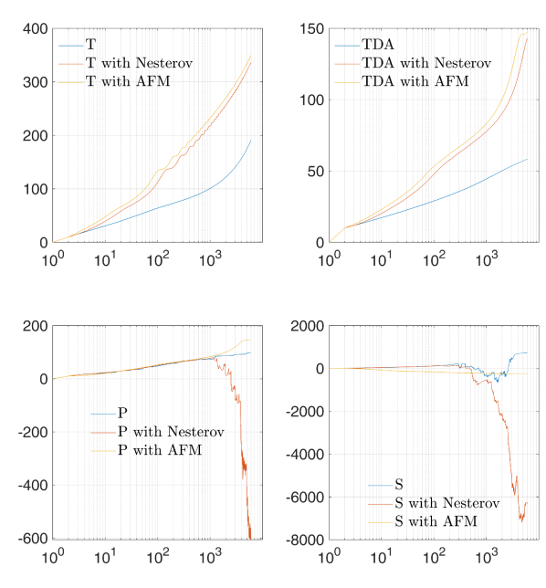
(a) Gaussian ($\sigma=1$)

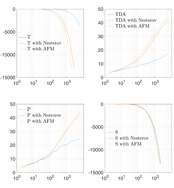
(b) Gaussian ($\sigma=5$)

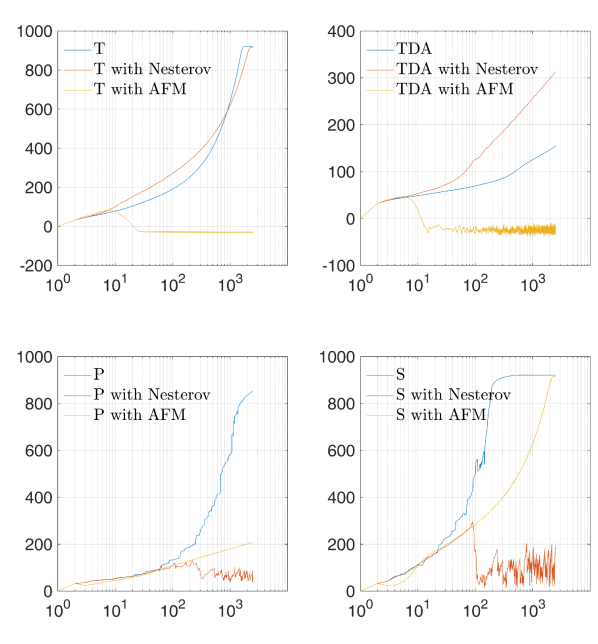
(c) Guided

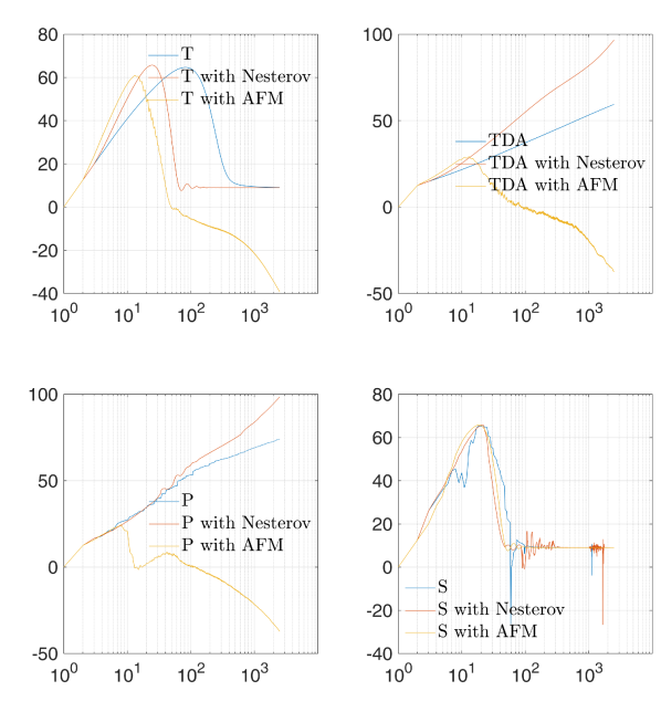
(d) Bilateral

Figure 12: Results of the T, TDA, P and S methods.

In Fig. 12, we compare the performance of these methods and their variants. A summary of the PSNR improvement properties is listed in Table 5. We can make the following observations.

1. The first row of the four sub-figures in Fig. 12 displays the results obtained without further acceleration by using either Nesterov or AFM methods. Among the tested methods, the three parametric Steffensen’s methods generally converge faster than their parameter-free counterparts in reversing the effects of a Gaussian filter with $\sigma=1$ and the guided filter. However, for the Gaussian filter with $\sigma=5$ and the bilateral filter, the results are mixed. For instance, although setting $\mu_{n}$ as the Chebyshev sequence yields the best results for most cases, it leads to a divergent result in reversing the effect of the bilateral filter using the method $\mathcal{{B}}_{1}$, which converges in the parameter-free case. Additionally, we observe that setting $\mu_{n}$ to "ed-1" or "ed-2" can enhance the convergence speed of the method $\mathcal{{C}}_{1}$ for both filters. Nevertheless, this setting may result in a divergent or inferior outcome compared to that of the corresponding parametric methods $\mathcal{{A}}_{1}$ and $\mathcal{{B}}_{1}$. Compared with the parametric counterpart, the parameter-free methods improve the PSNR all 4 filters at the cost of relatively slower speed.

2. The results obtained with Nesterov and AFM acceleration are shown in the second and third rows of the four sub-figures in Fig. 12. Generally, Nesterov acceleration outperforms AFM acceleration in terms of the number of cases of PSNR improvement, as summarized in Table 5 (b) and (c). For example, when reversing the effect of the guided filter, Nesterov acceleration improves the convergence speed of both parametric and parameter-free methods, albeit with a slight reduction in the percentage increase in PSNR compared to the case without acceleration, as demonstrated in the second row of Fig. 12 (c). On the other hand, the AFM acceleration does not lead to satisfactory results, as shown in the third row of Fig. 12 (c).

3. The parameter-free method without further acceleration is less likely to diverge. This is evident for the two difficult filters: Gaussian filter with $\sigma=5$ and the bilateral filter. Using Nesterov or AFM acceleration with both parametric and parameter-free methods can lead to divergent results in some cases, although the corresponding parameter-free methods converge. The cause of the problem can be shown as follows. When the iteration index $n$ is sufficiently large, the iteration $\boldsymbol{x}_{n+1}=\varphi(\boldsymbol{x}_{n})$ using Nesterov acceleration has the following two steps:

   $$\boldsymbol{u}_{n+1}=\varphi(\boldsymbol{x}_{n})$$ (72)

   and

   $$\boldsymbol{x}_{n+1}=2\boldsymbol{u}_{n+1}-\boldsymbol{u}_{n}$$ (73)

   which can be combined into one step

   $$\boldsymbol{u}_{n+1}=\varphi(2\boldsymbol{u}_{n}-\boldsymbol{u}_{n-1})$$ (74)

   Experimental results show that the convergence of the iteration $\boldsymbol{x}_{n+1}=\varphi(\boldsymbol{x}_{n})$ does not guarantee the convergence of (74). This issue deserves further investigation.

4. The performance of the parametric method with either Nesterov or AFM acceleration improves in some cases as the iteration progresses, as indicated by the increase in percentage PSNR improvement. However, there comes a point where the percentage PSNR improvement starts to decrease. This is also a problem for some parametric methods. Thus, further study is required to identify when to stop the iteration before the method’s performance deteriorates. To this end, non-referenced image quality assessment methods [44, 45] can be used to monitor the method’s performance.

method

$\mathcal{{A}}_{4}$

$\mathcal{{B}}_{4}$

$\mathcal{{C}}_{3}$

$\mu$

1

ed-1

ed-2

Cheby

1

ed-1

ed-2

Cheby

1

ed-1

ed-2

Cheby

Gauss-1

I

I

I

I

I

I

I

I

I

I

I

I

Guided

I

I

I

I

I

I

I

I

I

I

I

I

method

$\mathcal{{A}}_{1}$

$\mathcal{{B}}_{1}$

$\mathcal{{C}}_{1}$

$\mu$

1

ed-1

ed-2

Cheby

1

ed-1

ed-2

Cheby

1

ed-1

ed-2

Cheby

Gauss-5

I

I

I

I

I

I/F

I/F

I

I

I

I

I

Bilateral

I

I

I

I

I

I/F

I/F

I/F

I

I

I

I

(a) Results obtained without Nesterov or AFM acceleration.

method

$\mathcal{{A}}_{4}$

$\mathcal{{B}}_{4}$

$\mathcal{{C}}_{3}$

$\mu$

1

ed-1

ed-2

Cheby

1

ed-1

ed-2

Cheby

1

ed-1

ed-2

Cheby

Gauss-1

I

I

I

I/F

I

I

I

I/F

I

I

I

I/F

Guided

I

I

I

I

I

I

I

I

I

I

I

I

method

$\mathcal{{A}}_{1}$

$\mathcal{{B}}_{1}$

$\mathcal{{C}}_{1}$

$\mu$

1

ed-1

ed-2

Cheby

1

ed-1

ed-2

Cheby

1

ed-1

ed-2

Cheby

Gauss-5

I

F

F

F

I

F

F

F

I/F

I/F

I/F

F

Bilateral

I

I

I

I

I/F

I/F

I/F

I/F

I

I

I

I/F

(b) Results obtained by using Nesterov acceleration.

method|

$\mathcal{{A}}_{4}$

$\mathcal{{B}}_{4}$

$\mathcal{{C}}_{3}$

$\mu$

1

ed-1

ed-2

Cheby

1

ed-1

ed-2

Cheby

1

ed-1

ed-2

Cheby

Gauss-1

I

I

I/F

F

I

I/F

I/F

I

I

I

I

I/F

Guided

I

I/F

I/F

I/F

I/F

I/F

I/F

I

I

I/F

I/F

I/F

method

$\mathcal{{A}}_{1}$

$\mathcal{{B}}_{1}$

$\mathcal{{C}}_{1}$

$\mu$

1

ed-1

ed-2

Cheby

1

ed-1

ed-2

Cheby

1

ed-1

ed-2

Cheby

Gauss-5

F

F

F

F

I

F

F

F

I/F

I/F

I/F

F

Bilateral

I/F

I/F

I/F

I/F

I/F

I/F

I/F

I/F

I

I/F

I/F

I

(c) Result obtained from using AFM acceleration

Table 5: Summary of PSNR improvement for all cases presented in Fig. 12. "I" means improvement, "F" means no improvement or divergent, and "I/F" means unstable performance.

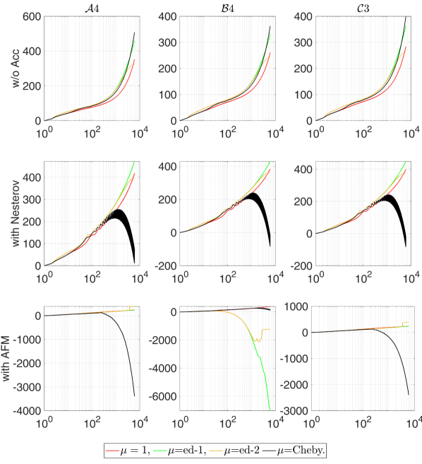
(a) Gaussian $\sigma=1$.

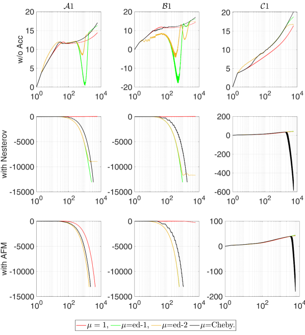
(b) Gaussian $\sigma=5$.

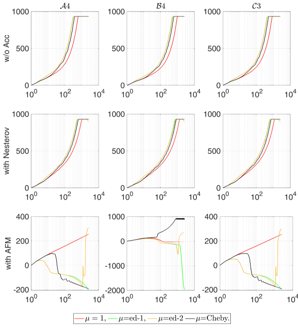
(c) Guided filter.

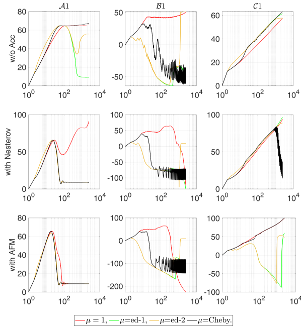
(d) Bilateral filter.

Figure 1: Comparison of the best performing methods in each category ($\mathcal{A}$, $\mathcal{B}$, $\mathcal{C}$) in inverting effects of 4 filters (a) Gaussian $\sigma=1$, (b) Gaussian $\sigma=5$, (c) Guided filter, and (d) Bilateral filter. Horizontal and vertical axis are the iteration index and percentage improvement of PSNR, respectively.

4.3 Comparison with best performing existing methods

To enable easy comparison with established techniques such as T-method [13], TDA-method [15], P-method and S-method [19], we select the top two performing methods. These methods are highlighted in Table 8, chosen based on their performance as detailed in the Supplementary Material. The criterion for the best performance is the highest percentage improvement in PSNR for all methods in reversing the effect of a filter at the end of a preset number of iterations.

	Vector variable Steffensen’s method			T, TDA, P, S
Gauss, $\sigma=1$	$\mathcal{{A}}_{4},\mu=$Cheby., (508)	$\mathcal{{B}}_{4},\mu=$ed-1, Nest., (430)	$\mathcal{{C}}_{3},\mu=$ed-1, Nest., (449)	T, AFM (350)	S (717)
Gauss. $\sigma=5$	$\mathcal{{A}}_{1},$ Nest., (40)	$\mathcal{{B}}_{1},$Nest., (40)	$\mathcal{{C}}_{1},\mu=$ed-1, AFM., (45)	TDA, AFM, (45)	P, AFM, (45)
Guided	$\mathcal{{A}}_{4}$ (933)	$\mathcal{{B}}_{4}$ (933)	$\mathcal{{C}}_{3}$ (933)	T (921)	S (920)
Bilateral	$\mathcal{{A}}_{1},$Nest., (91)	$\mathcal{{B}}_{1},\mu=$ed-2, (52)	$\mathcal{{C}}_{1},$AFM, (101)	TDA, Nest., (97)	P, Nest., (98)

Table 6: Best performing methods chosen based solely on the highest percentage of PSNR improvement when the method stops at the maximum number of preset iterations. Methods without specification of $\mu_{n}$ are with the setting $\mu_{n}=1$. The number in bracket, e.g., (508), indicates the 508% PSNR improvement. Nesterov acceleration is abbreviated as “Nest.”.

Comparison results are shown in Figures 2 and 3. We have the following observations.

1. For the Gaussian filter with $\sigma=1$, the performance of the S-method is unstable, but it has managed to converge to the highest improvement in PSNR. The three vector Steffensen’s methods have similar speed of improvement and is faster than that of the T-method. Except the S-method, the performance of all methods is on an increasing trajectory, which suggests potentially higher degree of improvement if more iterations are performed.

2. For the Gaussian filter with $\sigma=5$, at the end of the preset number of iterations, all methods have achieved PSNR improvement of about 40%, which is relatively small compared to the previous case. The TDA-method and the $\mathcal{C}_{1}$ method have a faster speed of improvement than that of other methods. The improvement of PSNR for all methods is trending upwards, indicating a possibility of further improvement if the iteration continues.

3. For the guided filter case, all methods converge to a similar level of PSNR improvement. The S-method has the fastest speed of convergence. The three Steffensen’s methods have similar speeds which are faster than that of the T-method. However, we note that in terms of computational complexity, the T-method is lowest, while the S-method is the highest.

4. For the bilateral filter case, the $\mathcal{{A}}_{1}$ method has the fastest speed of improvement. However, the improvement oscillates during the iteration. The performances of the other three method: TDA-method with Nesterov, P-method with Nesterov, and $\mathcal{{C}}_{1}$ method with AFM are similar. The speed of improvement of these method is slower than that of the $\mathcal{{A}}_{1}$ method at the start of the iteration. The $\mathcal{{B}}_{1}$ method is an exception, its performance deteriorates and then improves to achieves an PSNR improvement of about 50%.

5. The computational complexity of iterative image reverse filtering methods depends on two main factors: the number of calls to the black box filter (denoted N) and the complexity of the iteration process (denoted C). Table 7 presents a comparison of the methods examined in this section. The table also includes the running time of each method to complete a preset number of iterations, which is 2500 for the guided filter and 6000 for the Gaussian filter with $\sigma=1$. The running times for the other two filters are not shown because some methods diverge. The running times were obtained by averaging the results of 10 runs of each method programmed in MATLAB 2022b on a computer with an Intel i9-9900KF CPU and 64 GB of memory. The table reveals that the running times of the TDA method and the vector Steffensen’s method are about the same and roughly double that of the T-method. This is because the former two methods require 2 calls to the filter in 1 iteration, while the T-method requires only 1 call. However, the P-method and the S-method take significantly longer time to run due to the $O(n^{2})$ complexity involved in calculating the matrix 2-norm.

6. We would like to highlight that among 12 versions of the vector variable Steffensen’s methods, four methods stand out for their superior performance: $\mathcal{{A}}_{1}$, $\mathcal{{A}}_{4}$, $\mathcal{{B}}_{1}$, and $\mathcal{{C}}_{1}$. Importantly, these methods are novel and have not been published previously.

   	T [13]	TDA [15]	P [19]	S [19]	Steffensen
   N	1	2	2	2	2
   C	$O(n)$	$O(n)$	$O(n^{2})$	$O(n^{2})$	$O(n)$
   Guided	46.1	91.3	204.2	160.0	92.4
   Gauss-1	5.9	10.2	163.5	169.0	11.8

   
   

   Table 7: Rows 2 (number of filter calls) and 3 (complexity of vector/matrix operations) show the comparison of complexity of iterative methods studied in section 4.3, while rows 4 and 5 show the running time (seconds) to complete 2500 and 6000 iterations for each method to reverse the effects of a guided filter and a Gaussian filter with $\sigma=1$, respectively.

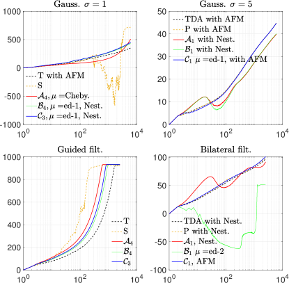
Figure 2: Comparison of the best performing vector variable Steffensen’s method with two best performing existing methods in inverting the effects of four filters. Horizontal and vertical axis are the iteration index and percentage improvement of PSNR, respectively..

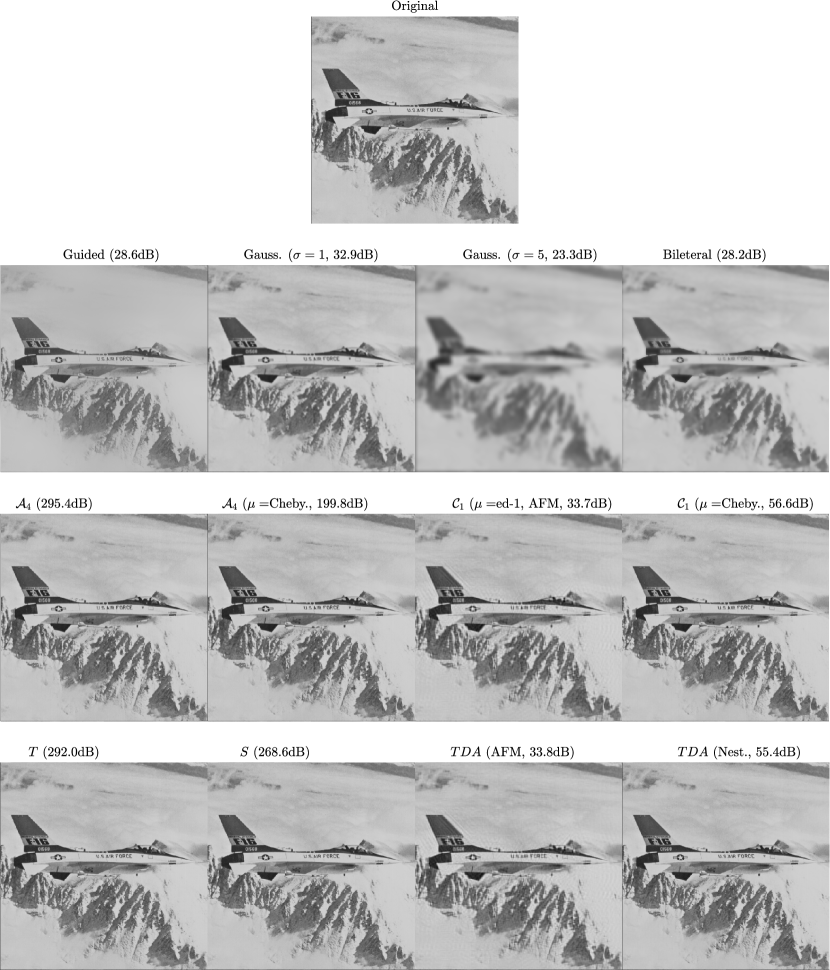
Figure 3: Comparison of best results in terms of achieving the highest PSNR when the method reaches the preset maximum number of iterations. The methods without specification of $\mu$ are with the setting $\mu=1$. The number in bracket, e.g., (28.5dB), indicates the PSNR of the image below. Nesterov acceleration is abbreviated as Nest.. Second row: images to be processed. Third row: best results of Steffensen’s method. Fourth row: best results of existing methods.

4.4 Summary and discussion

Comparing the proposed parameter-free and parametric Steffensen’s methods, the performance of the former is relatively more robust than that of the latter in that they are less likely to lead to divergent results. However, in some cases, the parametric methods actually achieve faster speed of PSNR improvement and thus a higher degree of improvement at the end of the preset number of iterations. When further acceleration methods such as the Nesterov and AFM are used, the results are mixed. Although in some cases both acceleration methods lead to faster speed of PSNR improvement, the Nesterov acceleration is preferred because with it the iteration is less likely to diverge. In addition, these two acceleration methods help to improve the performance for existing methods (T/TDA/P/S) in the two difficult cases: a Gaussian filter with $\sigma=5$ and a bilateral filter.

These mixed results highlight (1) the importance of a comprehensive study of the performance of variants of the proposed Steffensen’s method conducted in this work, and (2) the importance of this work which provides a new set of tools to tackle the reverse filtering problem. Further study should be conducted to explain why certain variants diverge in reversing the effect of a Gaussian filter with $\sigma=5$. An analysis of the convergence of T/TDA method using the Fourier transform was presented in [15].

5 Conclusions

This work is motivated by current research in solving the semi-blind image reverse filtering problem which can be formulated as a solving a system of nonlinear equations. We focus on extending Steffensen’s method to provide new tools for this problem. The first extension is the development of the parametric Steffensen’s method which can be regarded as an acceleration of the Mann iteration. The original Steffensen’s method is an acceleration of the Picard iteration. The second extension is the development of a family of 12 Steffensen’s methods for vector variables based on the notion of Brezinski inverse and the vector inverse defined by the geometric product. We have presented variants of these methods based on three ways of adaptively setting the parameter and using accelerated first-order method (which includes Nesterov method as a special case) to explore the possibility of further acceleration. To demonstrate the application to the semi-blind image reverse filtering problem, we present implementation details, analysis of computation complexity and convergence. We also show that some of the proposed methods generalize existing iterative algorithms. In the accompanying Supplementary Material, we have presented a comprehensive study of the performance of each of 108 variants of the vector Steffensen’s methods in terms of percentage improvement of PSNR at each iteration in reversing the effects of four commonly used filters in image processing. Based on these results, we have presented a detailed study of the best performing methods and compared them with the best performing existing methods. Overall, this paper provides a family of new Steffensen’s methods which are new tools for semi-blind image reverse filtering.

Supplementary information

We present a complete set of experimental results in the Supplementary Material, which outlines the experimental setup, presents a comprehensive collection of figures and tables, and provides detailed analysis of all the outcomes.

Appendix

Details of the vectorization of Steffensen’s method by using the notion of geometric product are shown below.

Case A1.1-G

$$\boldsymbol{\omega}_{n}=\boldsymbol{a}\boldsymbol{a}\boldsymbol{c}^{-1}=\frac{||\boldsymbol{a}||^{2}}{||\boldsymbol{c}||^{2}}\boldsymbol{c}$$

$$\boldsymbol{x}_{n+1}=\boldsymbol{x}_{n}+\frac{||\boldsymbol{a}||^{2}}{||\boldsymbol{c}||^{2}}\boldsymbol{c}$$

Case A1.2-G

$$\boldsymbol{\omega}_{n}=\boldsymbol{a}\boldsymbol{c}^{-1}\boldsymbol{a}=\frac{\boldsymbol{aca}}{||\boldsymbol{c}||^{2}}=\boldsymbol{a}+\frac{||\boldsymbol{a}||^{2}\boldsymbol{b}-||\boldsymbol{b}||^{2}\boldsymbol{a}}{||\boldsymbol{c}||^{2}}$$

$$\boldsymbol{x}_{n+1} =\boldsymbol{x}_{n}+\boldsymbol{a}+\frac{||\boldsymbol{a}||^{2}\boldsymbol{b}-||\boldsymbol{b}||^{2}\boldsymbol{a}}{||\boldsymbol{c}||^{2}}$$

$$=\phi(\boldsymbol{x}_{n})+\frac{||\boldsymbol{a}||^{2}\boldsymbol{b}-||\boldsymbol{b}||^{2}\boldsymbol{a}}{||\boldsymbol{c}||^{2}}$$

Case A2.1-G (same as A1.1-G)

$$\boldsymbol{\omega}_{n}=\boldsymbol{abc}^{-1}=\frac{\boldsymbol{abc}}{||\boldsymbol{c}||^{2}}=\frac{2(\boldsymbol{a^{T}b})\boldsymbol{a}-||\boldsymbol{a}||^{2}\boldsymbol{b}-||\boldsymbol{b}||^{2}\boldsymbol{a}}{||\boldsymbol{c}||^{2}}$$

$$\boldsymbol{x}_{n+1} =\phi(\boldsymbol{x}_{n})+\frac{2(\boldsymbol{a^{T}b})\boldsymbol{a}-||\boldsymbol{a}||^{2}\boldsymbol{b}-||\boldsymbol{b}||^{2}\boldsymbol{a}}{||\boldsymbol{c}||^{2}}$$

$$=\boldsymbol{x}_{n}+\boldsymbol{a}+\frac{2(\boldsymbol{a^{T}b})\boldsymbol{a}-||\boldsymbol{a}||^{2}\boldsymbol{b}-||\boldsymbol{b}||^{2}\boldsymbol{a}}{||\boldsymbol{c}||^{2}}$$

$$=\boldsymbol{x}_{n}+\frac{||\boldsymbol{a}||^{2}}{||\boldsymbol{c}||^{2}}\boldsymbol{c}$$

Case A2.2-G (same as A1.2-G)

$$\boldsymbol{\omega}_{n}=\boldsymbol{a}\boldsymbol{c}^{-1}\boldsymbol{b}=\frac{\boldsymbol{acb}}{||\boldsymbol{c}||^{2}}=\frac{||\boldsymbol{a}||^{2}\boldsymbol{b}-||\boldsymbol{b}||^{2}\boldsymbol{a}}{||\boldsymbol{c}||^{2}}$$

$$\boldsymbol{x}_{n+1}=\phi(\boldsymbol{x}_{n})+\frac{||\boldsymbol{a}||^{2}\boldsymbol{b}-||\boldsymbol{b}||^{2}\boldsymbol{a}}{||\boldsymbol{c}||^{2}}$$

Case A2.3-G (same as A1.2-G)

$$\boldsymbol{\omega}_{n}=\boldsymbol{b}\boldsymbol{c}^{-1}\boldsymbol{a}=\frac{\boldsymbol{bca}}{||\boldsymbol{c}||^{2}}=\frac{||\boldsymbol{a}||^{2}\boldsymbol{b}-||\boldsymbol{b}||^{2}\boldsymbol{a}}{||\boldsymbol{c}||^{2}}$$

Case A2.4-G

$$\boldsymbol{\omega}_{n}=\boldsymbol{ba}\boldsymbol{c}^{-1}=\frac{\boldsymbol{bac}}{||\boldsymbol{c}||^{2}}=\frac{||\boldsymbol{a}||^{2}\boldsymbol{b}-2(\boldsymbol{a^{T}b})\boldsymbol{b}+||\boldsymbol{b}||^{2}\boldsymbol{a}}{||\boldsymbol{c}||^{2}}$$

$$\boldsymbol{x}_{n+1} =\phi(\boldsymbol{x}_{n})+\frac{||\boldsymbol{a}||^{2}\boldsymbol{b}-2(\boldsymbol{a^{T}b})\boldsymbol{b}+||\boldsymbol{b}||^{2}\boldsymbol{a}}{||\boldsymbol{c}||^{2}}$$

$$=\phi(\phi(\boldsymbol{x}_{n}))-\boldsymbol{b}+\frac{||\boldsymbol{a}||^{2}\boldsymbol{b}-2(\boldsymbol{a^{T}b})\boldsymbol{b}+||\boldsymbol{b}||^{2}\boldsymbol{a}}{||\boldsymbol{c}||^{2}}$$

$$=\phi(\phi(\boldsymbol{x}_{n}))+\frac{||\boldsymbol{b}||^{2}}{||\boldsymbol{c}||^{2}}\boldsymbol{c}$$

Case A2.5-G (same as case A2.4-G)

$$\boldsymbol{\omega}_{n}=\boldsymbol{c}^{-1}\boldsymbol{a}\boldsymbol{b}=\frac{\boldsymbol{c}\boldsymbol{a}\boldsymbol{b}}{||\boldsymbol{c}||^{2}}=\frac{||\boldsymbol{a}||^{2}\boldsymbol{b}-2(\boldsymbol{a^{T}b})\boldsymbol{b}+||\boldsymbol{b}||^{2}\boldsymbol{a}}{||\boldsymbol{c}||^{2}}$$

Case A2.6-G (same as case A1.1-G)

$$\boldsymbol{\omega}_{n}=\boldsymbol{c}^{-1}\boldsymbol{b}\boldsymbol{a}=\frac{\boldsymbol{c}\boldsymbol{b}\boldsymbol{a}}{||\boldsymbol{c}||^{2}}=\frac{2(\boldsymbol{a}^{T}\boldsymbol{b})\boldsymbol{a}-||\boldsymbol{b}||^{2}\boldsymbol{a}-||\boldsymbol{a}||^{2}\boldsymbol{b}}{||\boldsymbol{c}||^{2}}$$

$$\boldsymbol{x}_{n+1} =\phi(\boldsymbol{x}_{n})+\frac{2(\boldsymbol{a}^{T}\boldsymbol{b})\boldsymbol{a}-||\boldsymbol{b}||^{2}\boldsymbol{a}-||\boldsymbol{a}||^{2}\boldsymbol{b}}{||\boldsymbol{c}||^{2}}$$

$$=\boldsymbol{x}_{n}+\boldsymbol{a}\frac{2(\boldsymbol{a}^{T}\boldsymbol{b})\boldsymbol{a}-||\boldsymbol{b}||^{2}\boldsymbol{a}-||\boldsymbol{a}||^{2}\boldsymbol{b}}{||\boldsymbol{c}||^{2}}$$

$$=\boldsymbol{x}_{n}+\frac{||\boldsymbol{a}||^{2}}{||\boldsymbol{c}||^{2}}\boldsymbol{c}$$

Case A3.1-G (same as A2.4-G)

$$\boldsymbol{\omega}_{n}=\boldsymbol{bb}\boldsymbol{c}^{-1}=\frac{||\boldsymbol{b}||^{2}}{||\boldsymbol{c}||^{2}}\boldsymbol{c}$$

$$\boldsymbol{x}_{n+1}=\phi(\phi(\boldsymbol{x}_{n}))+\frac{||\boldsymbol{b}||^{2}}{||\boldsymbol{c}||^{2}}\boldsymbol{c}$$

Case A3.2-G (same as A1.2-G)

$$\boldsymbol{\omega}_{n}=\boldsymbol{b}\boldsymbol{c}^{-1}\boldsymbol{b}=\frac{\boldsymbol{b}(\boldsymbol{a}-\boldsymbol{b})\boldsymbol{b}}{||\boldsymbol{c}||^{2}}=-\boldsymbol{b}+\frac{||\boldsymbol{a}||^{2}\boldsymbol{b}-||\boldsymbol{b}||^{2}\boldsymbol{a}}{||\boldsymbol{c}||^{2}}$$

$$\boldsymbol{x}_{n+1} =\phi(\phi(\boldsymbol{x}_{n}))-\boldsymbol{b}+\frac{||\boldsymbol{a}||^{2}\boldsymbol{b}-||\boldsymbol{b}||^{2}\boldsymbol{a}}{||\boldsymbol{c}||^{2}}$$

$$=\phi(\boldsymbol{x}_{n})+\frac{||\boldsymbol{a}||^{2}\boldsymbol{b}-||\boldsymbol{b}||^{2}\boldsymbol{a}}{||\boldsymbol{c}||^{2}}$$

Supplementary material

Introduction

The purpose of this document is to present all experimental findings that offer additional insights into the performance of the methods examined in the main paper for the task of reversing the effects of four commonly employed filters in image processing. For ease of comprehension, some information is duplicated in both this document and the main paper.

In this document, we present the test methods in section Test methods, and a comprehensive list of figures and tables is available in section Summary of figures and tables. Section Discussion of results includes a summary and analysis of all experimental outcomes, based on which we identify the best-performing methods for inverting the effects of the four image filters. Such methods are listed in section Best performing methods for inverting effects of the four filters. Finally, all figures and tables are presented at the end of this document.

Methodology and summary of figures and tables

Test methods

A comprehensive test has been conducted in the application of semi-blind reverse image filtering. Three frequently used filters are employed in this study: the Gaussian filter with $\sigma=1$ and $\sigma=5$, the guided filter with $r=35$ and $\epsilon=0.01$, and the bilateral filter with $\sigma_{s}=3$ and $\sigma_{r}=0.1$. While the Gaussian filter with $\sigma=1$ and $\sigma=5$ represent a lightly and heavily smoothing operation, the guided filter and the bilateral filter are two different types of edge-aware filters which smooth small-scale details and protect edges of large scale objects from smoothing.

The aim of this study is to evaluate the performance of vector Steffensen’s methods and corresponding acceleration versions by using the Nesterov method and adaptive first order method (AFM). The advantage of these two methods is that they are parameter free. Vector Steffensen’s methods studied in this work are listed as follows. Each category has the 12 variants.

1. Parameter free methods – results are presented in section Parameter-free methods and parametric methods..

   1. $\mu=1$.

   2. $\mu=1$ and Nesterov.

   3. $\mu=1$ and AFM.

2. Parametric methods – results are presented in section Parameter-free methods and parametric methods.

   1. $\mu_{n}=1+\exp(-((2n)/N)^{2})$, where $n$ and $N$ are the iteration index and total number of iterations, respectively. This method is called exponentially decay and is abbreviated as “ed-1”.

   2. $\mu_{n}=2\exp(-((2n)/N)^{2})$, where $n$ and $N$ are the iteration index and total number of iterations, respectively. This method is called exponentially decay and is abbreviated as “ed-2”.

   3. $\mu_{n}=2\min(1,\frac{1}{1+\cos(2(n+1)/P)})$, where $n$ and $P=64$ are the iteration index and the period of the Chebyshev sequence, respectively. This method is called Chebyshev sequence and is abbreviated as “Cheby.”

3. Parametric methods with Nesterov and AFM acceleration – results are presented in section Parametric methods with acceleration methods of Nesterov and AFM.

   1. “ed-1” with Nesterov.

   2. “ed-1” with AFM.

   3. “ed-2” with Nesterov.

   4. “ed-2” with AFM.

   5. “Cheby.” with Nesterov.

   6. “Cheby.” with AFM.

To evaluate the performance of the above methods, we also studies existing method such as T-method, TDA-method, P–method, and S-method and their corresponding acceleration by using the Nesterov method and the AFM method. Results are presented in section Performance of existing methods. A numerical comparison of the performance in improving PSNR is presented in section Best performing methods for inverting effects of the four filters.

All results are obtained by processing the gray scale “F-16” image of size $512\times 512$. The performance is measured by the percentage improvement in PSNR in each iteration:

$$p_{n}=\frac{PSNR_{n}-PSNR_{n}}{PSNR_{0}}\times 100\%$$

where $PSNR_{n}$ is the peak-signal-to-noise ratio of the filtered image and $PSNR_{n}$ is the PSNR of the inverse filtering result at the $n$th iteration.

Summary of figures and tables

Figures and Tables are summarized below in the order of their appearance.

• Figures 4 to 7 present results of PSNR improvement (vertical axis) versus iteration (horizontal axis) for the parametric-free methods without and with Nesterov or AFM acceleration. Results of parametric methods without accelerations are also presented in these figures.

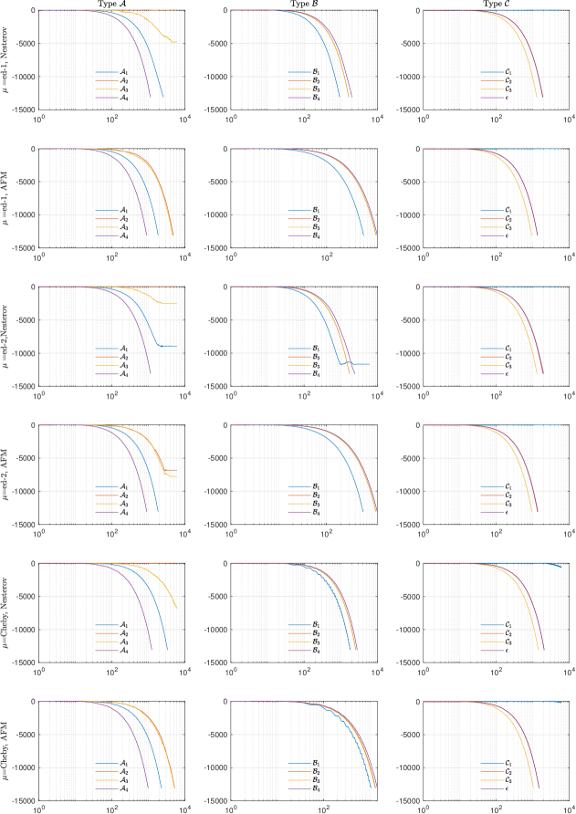
Figure 9: Results of Gaussian filter with $\sigma=5$.

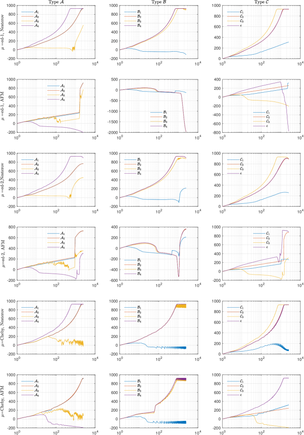
Figure 10: Results of guided filter.

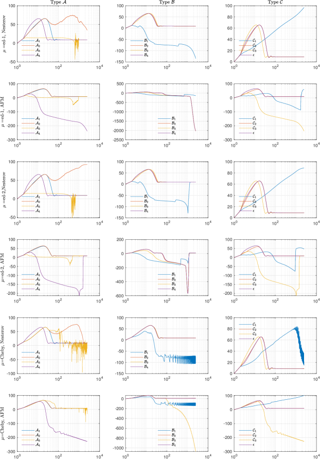
Figure 11: Results of bilateral filter.

• Figures 8-11 present results of parametric methods with accelerations.

• Tables 9-12 present results of percentage PSNR improvement at the end of the iteration for parameter-free and parametric method, with and without acceleration. The entry with “-” means the method is divergent.

• Figure 12 presents results of the 4 existing methods: T, TDA, P, and S.

• Table 13 presents results of percentage PSNR improvement at the end of the iteration for the 4 existing methods: T, TDA, P, and S. The entry with “-” means the method is divergent.

Discussion of results

Evaluation of the 12 vector Steffensen’s methods and their variants

Parameter-free methods and parametric methods.

Results for the parametric-free methods and parametric methods are presented in Figures 4 to 7. Key observations are summarized as follows.

1. Parametric-free methods (first 3 rows of Figures 4 to 7)

   1. Gaussian filter with $\sigma=1$.
      

      1. Without acceleration, it is shown in the first row of the figure that the top performers in each group are $\mathcal{{A}}_{4}$, $\mathcal{{B}}_{2-4}$, and $\mathcal{{C}}_{3}$. Among them $\mathcal{{A}}_{4}$ is better in terms of achieving the highest PSNR improvement.

      2. Results shown in the 2nd and 3rd row of the figure demonstrate that the two acceleration methods generally improve the speed of PSNR improvement for all methods.

      3. The Nesterov acceleration performs better than the AFM method in that it leads to better PSNR improvement at the end of the iteration for Types $\mathcal{A}$ and $\mathcal{C}$. For Type $\mathcal{B}$, the PSNR improvements are about the same for the two methods.

   2. Gaussian filter with $\sigma=5$.

      1. Only 5 methods results in improvement of PSNR:$\mathcal{{A}}_{1}$, $\mathcal{{A}}_{2},\mathcal{{A}}_{3},\mathcal{{B}}_{1}$, and $\mathcal{{C}}_{1}$. The improvement in PSNR is small (about 15%).

      2. Nesterov acceleration helps improve the speed of PSNR improvement for all convergent methods (increase from 15% to about 40%). The AFM acceleration leads to divergent results for all methods, except for $\mathcal{{C}}_{1}$.

   3. Guided filter.

      1. Without acceleration, the top performers in each group are $\mathcal{{A}}_{1,2,4}$, $\mathcal{{B}}_{2-4}$, and $\mathcal{{C}}_{3}$ and $\epsilon$. Among them $\mathcal{{A}}_{4}$ $\mathcal{{B}}_{4}$, and $\mathcal{{C}}_{3}$ are better in terms of speed of improvement.

      2. The Nesterov acceleration generally improves the speed for all methods. Results of using the AFM acceleration are mixed. While methods such as $\mathcal{{A}}_{3}$ and $\epsilon$ benefit from the acceleration, other methods such as the group $\mathcal{{B}}$ methods become divergent.

      3. The acceleration in convergence is at the cost of converging to a slightly lower improvement in PSNR than that without acceleration. For example, without acceleration the $\mathcal{A}_{1}$ method converges to 932% PSNR improvement. With Nesterov or AFM, the same method converges to 857% and 875%, respectively. We should point out that such differences are of no practical importance in this application, because the three PSNR improvements correspond to PSNR values of 295dB, 274dB and 279dB, respectively. The reverse filtering results in these three cases are effectively the same as the original image.

   4. Bilateral filter.

      1. Only 5 methods lead to PSNR improvement:$\mathcal{{A}}_{1}$, $\mathcal{{A}}_{2},\mathcal{{A}}_{3},\mathcal{{B}}_{1}$, and $\mathcal{{C}}_{1}$. The improvement in PSNR is modest (about 60%).

      2. Both acceleration methods fail to improve the speed. The exception is method $\mathcal{{C}}_{1}$ for which the two acceleration methods lead to the faster speed of improvement.

   5. Summary. Among the tested methods, $\mathcal{{A}}{4}$, $\mathcal{{B}}{4}$, and $\mathcal{{C}}{3}$ were found to be the most effective for reversing the effects of two filters, namely Gaussian with $\sigma=1$ and guided filter, which are relatively easy to reverse. On the other hand, for two filters, namely Gaussian with $\sigma=5$ and bilateral filter, which are more difficult to reverse, the top-performing methods were $\mathcal{{A}}{1}$, $\mathcal{{B}}{1}$, and $\mathcal{{C}}{1}$. Such observations will be used in the main paper as the basis to compare different vector Steffensen’s methods and their variants.

2. Parametric methods (row 4 to row 6 in Figures 4 to 7).
   In general, the list of methods, that result in PSNR improvement, is the same as that in the parametric-free case.

   1. Gaussian filter with $\sigma=1$.

      1. The methods “ed-1” and “Cheby.” appear to produce comparable or superior performance to parametric-free methods in terms of speed of PSNR improvement. For example, method $\mathcal{A}_{4}$ with $\mu=$ed-1 and $\mu=$Cheby. achieves 460% and 508% PSNR improvement, respectively. In contrast, the same method with $\mu=1$ (parameter-free setting) achieves 352%.

      2. The method “ed-2” is inferior to “ed-1” and “Cheby.” and its performance is not as good as that the parameter-free case.

      3. In general, the parametric-free methods with Nesterov or AFM achieve better PSNR improvement than those corresponding parametric methods.

   2. Gaussian filter with $\sigma=5$.

      1. The methods “ed-1”, “ed-2” and “Cheby.” appear to produce comparable performance to parametric-free methods in terms of speed of PSNR improvement. There is no benefit of using these method.

   3. Guided filter

      1. The methods “ed-1”, “ed-2” and “Cheby.” appear to produce comparable performance to parametric-free methods in terms of speed PSNR improvement.

      2. There are a few exceptions. (1) The $\mathcal{A}_{3}$ method with “ed-1” and “ed-2” lead to far worse result than the corresponding method without using the parameter. (2) while “ed-1” and “Cheby.” make the method $\mathcal{{B}}_{1}$ divergent, “ed-2” significantly improves the PSNR improvement of $\mathcal{{B}}_{1}$ from the parameter-free case of 109% to 318%. (3) “ed-2” makes $\mathcal{{B}}_{2}$ divergent.

   4. Bilateral filter

      1. The methods “ed-1”, “ed-2” and “Cheby.” appear to produce comparable performance to parametric-free methods in terms of speed of PSNR improvement.

      2. The exception is that both “ed-1” and “Cheby.” make the method $\mathcal{{B}}_{1}$ divergent.

Parametric methods with acceleration methods of Nesterov and AFM

Results for the accelerated parametric methods are presented in Figures 8 to 11. Comparing the two groups of figures (Figures 4-7 and Figures8-11) we have the following observations.

1. Gaussian filter with $\sigma=1$.

   1. The Type $\mathcal{A}$ and $\mathcal{C}$ methods with “ed-1” or “ed-2” settings and Nesterov or AFM acceleration outperform or match performance of the parametric-free methods in terms of PSNR improvement at the end of the iteration. However, the “Cheby” setting with Nesterov or AFM acceleration leads to divergence or worse results.

   2. For the Type $\mathcal{B}$ methods, only the setting of “ed-1” together with Nesterov acceleration have produces about the same or better results than parametric-free methods in terms of PSNR improvement at the end of the iteration. Other combinations of parameter setting and acceleration lead to either inferior or divergent results.

2. Gaussian filter with $\sigma=5$.

   1. The settings “ed-1” or “ed-2” together with Nesterov or AFM acceleration have produced comparable performance to parametric-free methods in terms of PSNR improvement at the end of the iteration.

   2. Other combinations of parameter setting and acceleration lead to either inferior or divergent results.

3. Guided filter

   1. Only the two methods $\mathcal{{B}}_{1}$ and $\mathcal{{C}}_{1}$ have benefited from combinations of one of the three parameter settings together with the acceleration methods (Nesterov and AFM). Using such combinations, all other methods have produced comparable or inferior results. As such, there is no benefit of using further accelerations in this case.

4. Bilateral filter

   1. The methods “ed-1”, “ed-2” and “Cheby.” appear to produce comparable performance to parametric-free methods in terms of speed of convergence and PSNR improvement. The exception is that both “ed-1” and “Cheby.” make the method $\mathcal{{B}}_{1}$ divergent.

Performance of existing methods

Results for the 4 existing methods are presented in Fig. 12 and Table 13. We can summarize results as follows.

1. Gaussian filter with $\sigma=1$.

   1. The S-method is a clear winner in terms of achieving the highest PSNR improvement.

   2. The two acceleration methods improve the convergence speed of the T-method, but the impact on other methods is mixed. Specifically, the Nesterov acceleration can cause the P-method and S-method to diverge, while the AFM method cause the S-method to diverge.

2. Gaussian filter with $\sigma=5$.

   1. Only the TDA-method and P-method have shown PSNR improvement as the iteration progresses. The T-method and the S-method fail to improve the PSNR.

   2. The two acceleration methods substantially improves the speed of PSNR improvement of the TDA-method and the P-method.

   3. The TDA-method is the overall winner due to is low computational complexity compared to that of the P-method.

3. Guided filter

   1. The T-method and S-method have achieved about the same PSNR improvement. However, the T-method is preferred because of its low computational complexity.

   2. The Nesterov acceleration only improves the performance of the TDA method, and it causes other methods to produce inferior results compared to those without the acceleration.

   3. The AFM acceleration have a negative impact on all four methods.

4. Bilateral filter

   1. Both the T-method and S-method exhibit PSNR improvements that peaks at 9%. In contrast, the TDA-method and P-method show a PSNR improvement peak at around 97%.

   2. The Nesterov acceleration has a positive effect on the speed of PSNR improvement, while the AFM acceleration has a negative impact on the T, P, and TDA methods and has only a minor effect on the S-method.

Best performing methods for inverting effects of the four filters

From the above results, the best performing methods for reversing effects of each filter are listed in the following Table 8. A detailed discussion of results due to these methods are presented in the main paper.

	Vector variable Steffensen’s method			T, TDA, P, S
Gauss-1	$\mathcal{{A}}_{4},\mu=$Cheby., (508)	$\mathcal{{B}}_{4},\mu=$ed-1, Nest., (430)	$\mathcal{{C}}_{3},\mu=$ed-1, Nest., (449)	T, AFM (350)	S (717)
Gauss-5	$\mathcal{{A}}_{1},$ Nest., (40)	$\mathcal{{B}}_{1},$Nest., (40)	$\mathcal{{C}}_{1},\mu=$ed-1, AFM., (45)	TDA, AFM, (45)	P, AFM, (45)
Guided	$\mathcal{{A}}_{4}$ (933)	$\mathcal{{B}}_{4}$ (933)	$\mathcal{{C}}_{3}$ (933)	T (921)	S (920)
Bilateral	$\mathcal{{A}}_{1},$Nest., (91)	$\mathcal{{B}}_{1},\mu=$ed-2, (52)	$\mathcal{{C}}_{1},$AFM, (101)	TDA, Nest., (97)	P, Nest., (98)

Table 8: Best performing methods chosen based solely on the highest percentage of PSNR improvement when the method stops at the maximum number of preset iterations. Methods without specification of $\mu_{n}$ are with the setting $\mu_{n}=1$. The number in bracket, e.g., (508), indicates the 508% PSNR improvement at the end of the iteration. Nesterov acceleration is abbreviated as Nest..

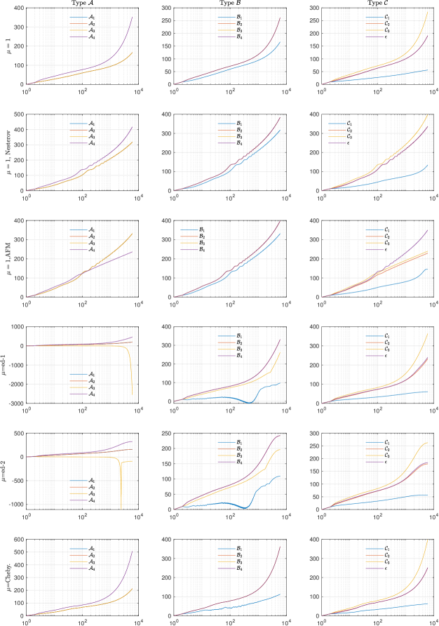
Figure 4: Results of Gaussian filter with $\sigma=1$.

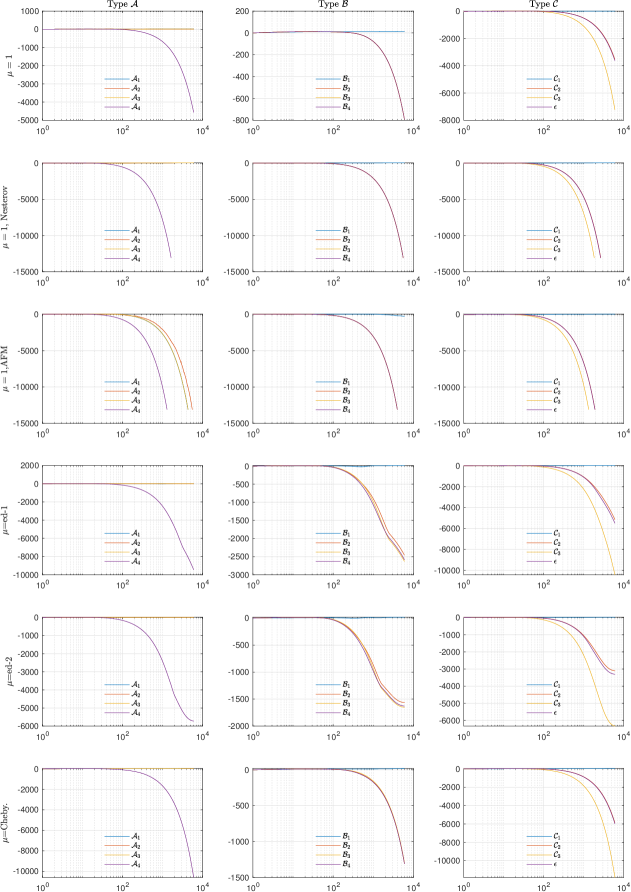
Figure 5: Results of Gaussian filter with $\sigma=5$.

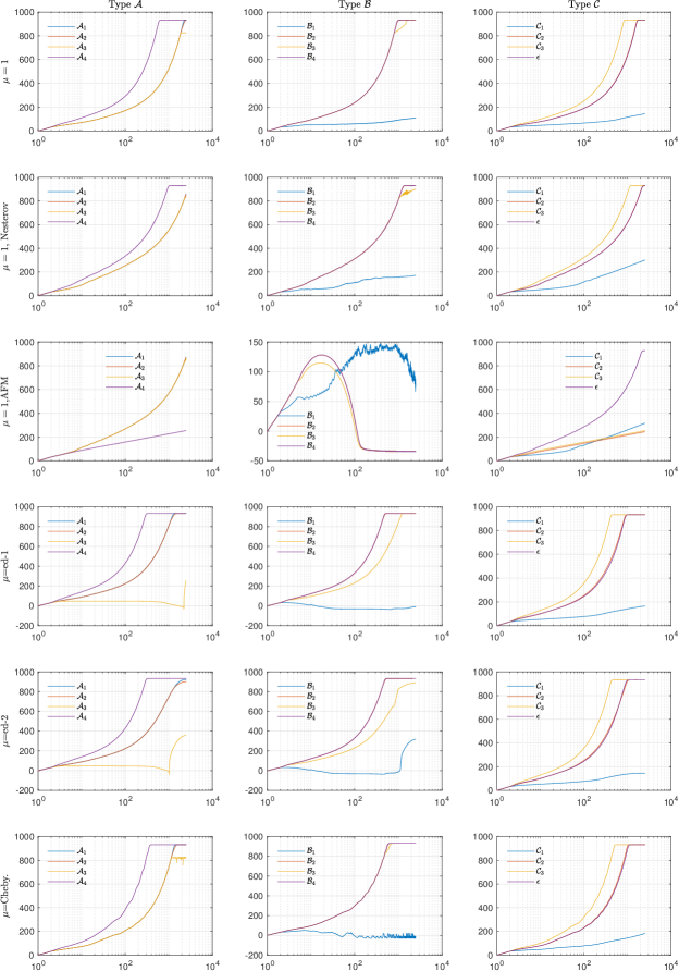
Figure 6: Results of guided filter.

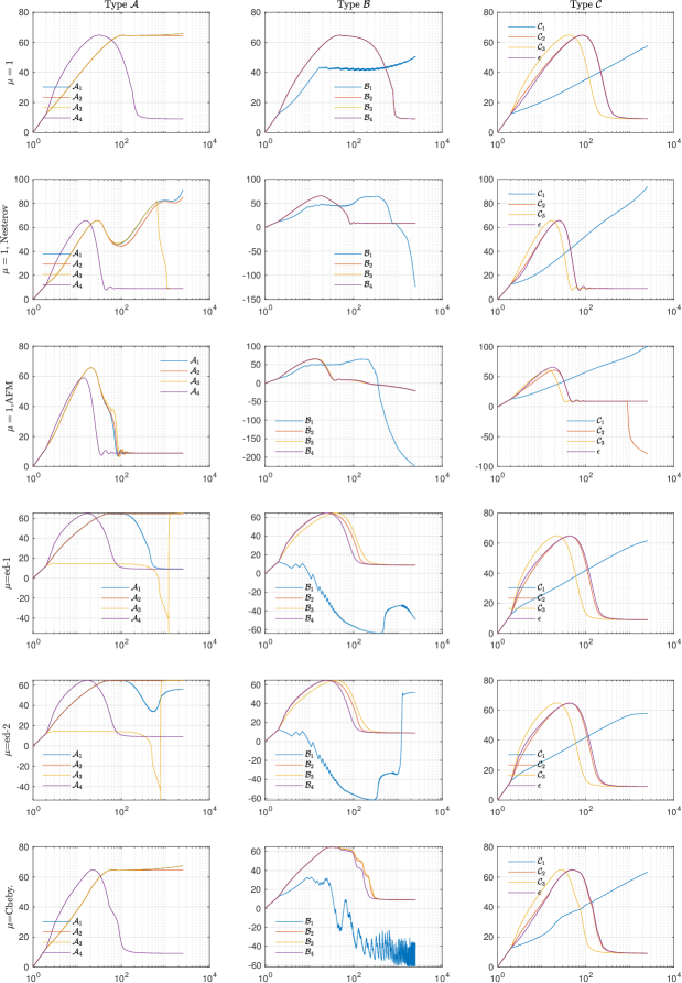
Figure 7: Results of bilateral filter.

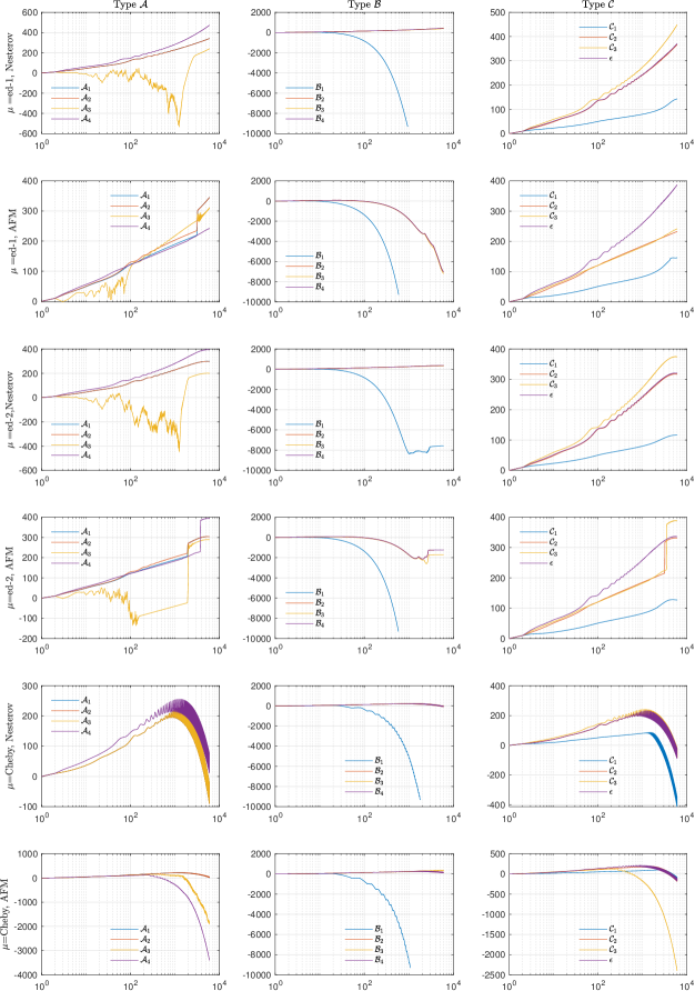
Figure 8: Results of Gaussian filter with $\sigma=1$.

	$\mathcal{A}_{1}$	$\mathcal{A}_{2}$	$\mathcal{A}_{3}$	$\mathcal{A}_{4}$	$\mathcal{B}_{1}$	$\mathcal{B}_{2}$	$\mathcal{B}_{3}$	$\mathcal{B}_{4}$	$\mathcal{C}_{1}$	$\mathcal{C}_{2}$	$\mathcal{C}_{3}$	$\epsilon$
$\mu=1$	166	166	166	352	166	261	261	261	56	191	284	191
$\mu=1$, Nest.	317	317	317	417	317	383	383	383	134	336	398	336
$\mu=1$, AFM	331	331	331	236	331	398	398	398	146	229	240	349
$\mu$=ed1	199	199	-	460	98	331	262	331	61	233	364	240
$\mu=$ed2	157	157	-	323	109	242	196	242	57	179	263	184
$\mu$=Cheby	213	213	213	508	112	362	362	362	63	251	399	252
ed1+Nest.	341	341	240	472	-	430	388	430	143	367	449	370
ed1+AFM	345	345	310	242	-	-	-	-	146	232	242	387
ed2+Nest.	299	298	200	394	-	360	336	360	117	317	375	320
ed2+AFM	304	304	290	394	-	-	-	-	127	331	388	336
Cheby.+Nest.	-	-	-	57	-	-	-	-	-	-	-	-
Cheby.+AFM	40	43	-	-	-	144	354	133	-	-	-	-

Table 9: Percentage of PSNR improvement at the end of iteration for the Gaussian filter $\sigma=1$. The entry with "-" means the method is divergent.

	$\mathcal{A}_{1}$	$\mathcal{A}_{2}$	$\mathcal{A}_{3}$	$\mathcal{A}_{4}$	$\mathcal{B}_{1}$	$\mathcal{B}_{2}$	$\mathcal{B}_{3}$	$\mathcal{B}_{4}$	$\mathcal{C}_{1}$	$\mathcal{C}_{2}$	$\mathcal{C}_{3}$	$\epsilon$
$\mu=1$	14	12	14	-	14	-	-	-	16	-	-	-
$\mu=1$, Nest.	40	39	40	-	40	-	-	-	41	-	-	-
$\mu=1$, AFM	-	-	-	-	-	-	-	-	44	-	-	-
$\mu$=ed1	16	12	12	-	16	-	-	-	19	-	-	-
$\mu=$ed2	15	12	13	-	15	-	-	-	17	-	-	-
$\mu$=Cheby	17	12	17	-	17	-	-	-	20	-	-	-
ed1+Nest.	-	25	-	-	-	-	-	-	43	-	-	-
ed1+AFM	-	-	-	-	-	-	-	-	45	-	-	-
ed2+Nest.	-	21	-	-	-	-	-	-	40	-	-	-
ed2+AFM	-	-	-	-	-	-	-	-	42	-	-	-
Cheby.+Nest.	-	-	-	-	-	-	-	-	-	-	-	-
Cheby.+AFM	-	-	-	-	-	-	-	-	-	-	-	-

Table 10: Percentage of PSNR improvement at the end of iteration for the Gaussian filter $\sigma=5$. The entry with "-" means the method is divergent

	$\mathcal{A}_{1}$	$\mathcal{A}_{2}$	$\mathcal{A}_{3}$	$\mathcal{A}_{4}$	$\mathcal{B}_{1}$	$\mathcal{B}_{2}$	$\mathcal{B}_{3}$	$\mathcal{B}_{4}$	$\mathcal{C}_{1}$	$\mathcal{C}_{2}$	$\mathcal{C}_{3}$	$\epsilon$
$\mu=1$	932	930	825	933	109	933	933	933	145	933	933	933
$\mu=1$, Nest.	857	855	833	930	172	931	899	930	301	928	930	929
$\mu=1$, AFM	875	872	851	255	75	-	-	-	318	245	255	927
$\mu$=ed1	933	933	258	933	-	933	933	933	166	933	933	933
$\mu=$ed2	923	902	359	933	318	-	890	933	144	933	933	932
$\mu$=Cheby	933	933	825	933	-	933	933	933	183	933	933	933
ed1+Nest.	927	927	558	930	-	930	902	930	313	927	930	929
ed1+AFM	921	919	772	-	-	-	-	-	322	261	-	-
ed2+Nest.	766	766	448	893	214	893	872	893	258	887	893	890
ed2+AFM	727	726	352	308	210	367	356	363	264	875	301	889
Cheby.+Nest.	927	927	26	930	-	929	844	930	59	928	930	929
Cheby.+AFM	924	923	78	-	-	927	921	927	322	246	-	927

Table 11: Percentage of PSNR improvement at the end of iteration for the guided filter. The entry with "-" means the method is divergent.

	$\mathcal{A}_{1}$	$\mathcal{A}_{2}$	$\mathcal{A}_{3}$	$\mathcal{A}_{4}$	$\mathcal{B}_{1}$	$\mathcal{B}_{2}$	$\mathcal{B}_{3}$	$\mathcal{B}_{4}$	$\mathcal{C}_{1}$	$\mathcal{C}_{2}$	$\mathcal{C}_{3}$	$\epsilon$
$\mu=1$	66	64	66	9	50	9	9	9	58	9	9	9
$\mu=1$, Nest.	91	85	9	9	-	9	9	9	94	9	9	9
$\mu=1$, AFM	9	9	9	9	-	-	-	-	101	-	9	9
$\mu$=ed1	9	64	65	9	-	9	9	9	62	9	9	9
$\mu=$ed2	56	65	65	9	52	9	9	9	58	9	9	9
$\mu$=Cheby	67	64	67	9	-	9	9	9	63	9	9	9
ed1+Nest.	9	34	9	9	-	9	9	9	97	9	9	9
ed1+AFM	9	9	9	-	-	-	-	-	60	9	-	9
ed2+Nest.	9	92	9	9	9	9	9	9	89	9	9	9
ed2+AFM	9	9	9	9	9	9	9	9	47	9	9	9
Cheby.+Nest.	9	9	13	9	-	9	9	9	14	9	9	9
Cheby.+AFM	9	9	-3	-	-	9	-	9	101	9	-	9

Table 12: Percentage of PSNR improvement at the end of iteration for the bilateral filter. The entry with "-" means the method is divergent.

	T	TDA	P	S
w/o Acc	191	58	98	717
with Nest.	336	143	-	-
with AFM	350	148	148	-

(a) Gaussian filter $\sigma=1$.

	T	TDA	P	S
w/o Acc	-	17	24	-
with Nest.	-	42	43	-
with AFM	-	45	45	-

(b) Gaussian filter $\sigma=5$.

	T	TDA	P	S
w/o Acc	921	155	854	920
with Nest.	918	313	60	187
with AFM	-	-	208	916

(c) Guided filter.

	T	TDA	P	S
w/o Acc	9	59	74	9
with Nest.	9	97	98	9
with AFM	-	-	-	9

(d) Bilateral filter.

Table 13: Percentage of PSNR improvement at the end of iteration T/TDA/P/S methods. The entry with "-" means the method is divergent.

References

- [1] A. Ostrowski, Solution of Equations and Systems of Equations, 2nd Ed. Academic Press, 1966.
- [2] A. Aitken, “XXV.– On Bernoulli’s numerical solution of algebraic equations,” Proc. Roy. Soc., Edinburgh, pp. 289 – 305, 1927.
- [3] J. Steffensen, “Remarks on iteration,” Scandinavian Actuarial Journal, vol. 1933, no. 1, pp. 64–72, 1933.
- [4] D. G. Anderson, “Iterative procedures for nonlinear integral equations,” J. ACM, vol. 12, pp. 547–560, 1965.
- [5] P. Wynn, “Acceleration techniques for iterated vector and matrix problems,” Math. Comput., vol. 16, no. 79, pp. 301–322, 1962.
- [6] F. Bornemann, D. Laurie, S. Wagon, and J. Waldvogel, The SIAM 100-Digit Challenge A Study in High-Accuracy Numerical Computing. SIAM, 2004.
- [7] C. Brezinski, “Convergence acceleration during the 20th century,” J. Comput. Appl. Math, vol. 122, pp. 1–21, 2000.
- [8] M. J. Kochenderfer and T. A. Wheeler, Algorithms for Optimization. The MIT Press, 2019.
- [9] J. Zhang, B. O’Donoghue, and S. P. Boyd, “Globally convergent type-I Anderson acceleration for nonsmooth fixed-point iterations,” SIAM J. Optim., vol. 30, pp. 3170–3197, 2020.
- [10] J. Chen, M. Gan, Q. Zhu, P. Narayan, and Y. Liu, “Robust standard gradient descent algorithm for ARX models using Aitken acceleration technique,” IEEE Trans. Cybern., pp. 1–10, 2021.
- [11] T. Wadayama and S. Takabe, “Chebyshev periodical successive over-relaxation for accelerating fixed-point iterations,” IEEE Signal Process Lett, vol. 28, pp. 907–911, 2021.
- [12] Z. Li and J. Li, “A fast Anderson-Chebyshev acceleration for nonlinear optimization,” in Proc. 23rd Int. Conf. AI and Statistics, pp. 1047–1057, 2020.
- [13] X. Tao, C. Zhou, X. Shen, J. Wang, and J. Jia, “Zero-order reverse filtering,” in Proc. IEEE ICCV, pp. 222–230, 2017.
- [14] P. Milanfar, “Rendition: Reclaiming what a black box takes away,” SIAM J. Imaging Sci., vol. 11, no. 4, pp. 2722–2756, 2018.
- [15] F. J. Galetto and G. Deng, “Reverse image filtering using total derivative approximation and accelerated gradient descent,” IEEE Access, vol. 10, pp. 124928–124944, Dec. 2022.
- [16] A. G. Belyaev and P.-A. Fayolle, “Black-box image deblurring and defiltering,” Signal Process. Image Commun., vol. 108, p. 116833, 2022.
- [17] L. Wang, P.-A. Fayolle, and A. G. Belyaev, “Reverse image filtering with clean and noisy filters,” Signal, Image and Video Process., vol. 17, pp. 333–341, 2022.
- [18] M. Delbracio, I. Garcia-Dorado, S. Choi, D. Kelly, and P. Milanfar, “Polyblur: Removing mild blur by polynomial reblurring,” IEEE Trans Comput Imaging, vol. 7, pp. 837–848, 2021.
- [19] A. G. Belyaev and P.-A. Fayolle, “Two iterative methods for reverse image filtering,” Signal, Image and Video Process., pp. 1–9, 2021.
- [20] P. Wynn, “The epsilon algorithm and operational formulas of numerical analysis,” Math. Comput., vol. 15, no. 74, pp. 151–158, 1961.
- [21] J. E. Gentle, Matrix Algebra Theory, Computations and Applications in Statistics Second Edition. Springer Texts in Statistics, 2017.
- [22] C. Brezinski, Accèlèration de la convergence en analyse numèrique. Springer-Verlag, 1977.
- [23] A. Sidi, Vector Extrapolation Methods with Applications. SIAM, 2017.
- [24] A. J. Macleod, “Acceleration of vector sequences by multi-dimensional a2 methods,” Commun Appl. Numer. Methods, vol. 2, pp. 385–392, 1986.
- [25] I. Ramiére and T. Helfer, “Iterative residual-based vector methods to accelerate fixed point iterations,” Comput. Math. with Appl., vol. 70, pp. 2210–2226, 2015.
- [26] G. Deng and F. J. Galetto, “Fast iterative reverse filters using fixed-point acceleration,” Signal Image Video Process., Apr. 2023, Accepted.
- [27] C. Kelley, Iterative Methods for Linear and Nonlinear Equations. SIAM, 1995.
- [28] W. R. Mann, “Mean value methods in iteration,” Proc. Am. Math. Soc., vol. 4, pp. 506–510, 1953.
- [29] S. Gull, A. Lasenby, and C. Doran, “Imaginary numbers are not real–the geometric algebra of spacetime,” Found. Phys., vol. 23, pp. 1175–1201, 1993.
- [30] D. Kim and J. A. Fessler, “Adaptive restart of the optimized gradient method for convex optimization,” J. Optim. Theory Appl., vol. 178, pp. 240–263, 2018.
- [31] Y. Nesterov, “A method for unconstrained convex minimization problem with the rate of convergence o(1/),” Dokl. Akad. Nauk. USSR, vol. 269, pp. 543–547, 1983.
- [32] A. Beck and M. Teboulle, “A fast iterative shrinkage-thresholding algorithm for linear inverse problems,” SIAM J. Imaging Sci., vol. 2, pp. 183–202, 2009.
- [33] D. Borwein and J. Borwein, “Fixed point iterations for real functions,” J. Math. Anal. Appl., vol. 157, pp. 112–126, 1991.
- [34] D. A. Smith, W. F. Ford, and A. Sidi, “Extrapolation methods for vector sequences,” SIAM Review, vol. 29, no. 2, pp. 199–233, 1987.
- [35] C. Lemaréchal, “Une méthode de résolution de certains systèmes non linéaires bien posés,” CR Acad. Sci. Paris, sér. A, vol. 272, pp. 605–607, 1971.
- [36] G. Sedogbo, “Some convergence acceleration processes for a class of vector sequences,” Applicationes Mathematicae, vol. 24, no. 3, pp. 299–306, 1997.
- [37] A. Jennings, “Accelerating the convergence of matrix iterative processes,” IMA J. Appl. Math., vol. 8, pp. 99–110, 1971.
- [38] B. M. Irons and R. C. Tuck, “A version of the Aitken accelerator for computer iteration,” Int. J. Numer. Methods Eng., vol. 1, no. 3, pp. 275–277, 1969.
- [39] O. C. Zienkiewicz and R. Löhner, “Accelerated ’relaxation’ or direct solution? Future prospects for FEM,” Int. J. Numer. Methods Eng., vol. 21, pp. 1–11, 1985.
- [40] P. R. Graves-Morris, “Extrapolation methods for vector sequences,” Numerische Mathematik, vol. 61, pp. 475–487, 1992.
- [41] S. Ishikawa, “Fixed points by a new integration method,” Proc. Am. Math. Soc., vol. 44, pp. 147–150, 1974.
- [42] S. Hassan, M. D. la Sen, P. Agarwal, Q. Ali, and A. Hussain, “A new faster iterative scheme for numerical fixed points estimation of Suzuki’s generalized nonexpansive mappings,” Math. Probl. Eng., vol. 2020, pp. 1–9, 2020.
- [43] S. Kassam and H. Poor, “Robust techniques for signal processing: A survey,” Proc. IEEE, vol. 73, pp. 433–481, 1985.
- [44] V. Hosu, H. Lin, T. Szirányi, and D. Saupe, “Koniq-10k: An ecologically valid database for deep learning of blind image quality assessment,” vol. 29, pp. 4041–4056, 2019.
- [45] W. Zhang, K. Ma, J. Yan, D. Deng, and Z. Wang, “Blind image quality assessment using a deep bilinear convolutional neural network,” vol. 30, pp. 36–47, 2019.