Learning Causally Disentangled Representations via the Principle of Independent Causal Mechanisms

Abstract

Learning disentangled causal representations is a challenging problem that has gained significant attention recently due to its implications for extracting meaningful information for downstream tasks. In this work, we define a new notion of causal disentanglement from the perspective of independent causal mechanisms. We propose ICM-VAE, a framework for learning causally disentangled representations supervised by causally related observed labels. We model causal mechanisms using learnable flow-based diffeomorphic functions to map noise variables to latent causal variables. Further, to promote the disentanglement of causal factors, we propose a causal disentanglement prior that utilizes the known causal structure to encourage learning a causally factorized distribution in the latent space. Under relatively mild conditions, we provide theoretical results showing the identifiability of causal factors and mechanisms up to permutation and elementwise reparameterization. We empirically demonstrate that our framework induces highly disentangled causal factors, improves interventional robustness, and is compatible with counterfactual generation.

1 Introduction

Disentangled representation learning aims to learn meaningful and compact representations that capture semantic aspects of data by structurally disentangling the factors of variation [1]. Such representations have been shown to offer useful properties such as better interpretability, robustness to distribution shifts, efficient out-of-distribution sampling, and fairness [2]. However, disentangled representation learning typically assumes that the underlying factors are independent, which is unrealistic in practice. The factors generating the data can contain correlations or even causal relationships that are disregarded when factors are assumed to be independent. Further, a generative model learning from an independent prior assumes that all combinations of the latent factors are equally likely to appear in the training data. Thus, disentangling the factors would yield a sub-optimal likelihood since the assumed support could be well outside the support of the training data.

Recently, there has been a growing interest in bridging causality [3] and representation learning [1]. The goal of causal representation learning is to map unstructured low-level data to high-level abstract causal variables of interest [4]. The key assumption is that high-dimensional observations are generated from a set of underlying low-dimensional causally related factors of variation. Causal representations also adhere to the principle of independent causal mechanisms (ICM) [5], which states that the mechanisms that generate each causal variable are independent such that a change in one mechanism does not affect another [6, 7].

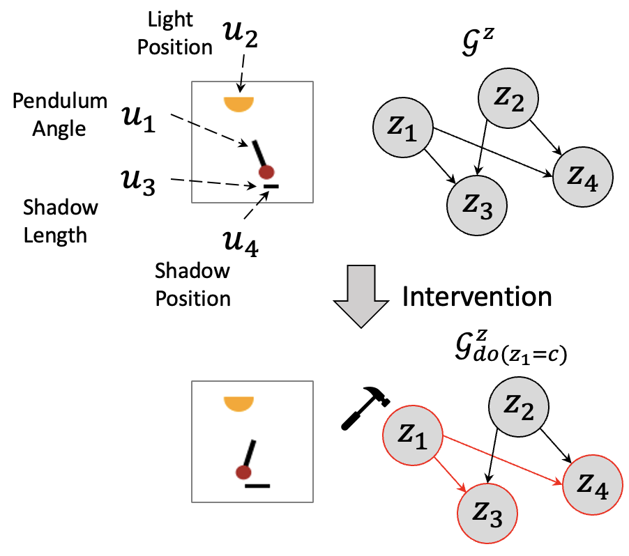
Figure 1: We learn causal models representing images as causal variables $z$. The bottom shows the effect of intervening on the pendulum’s angle and generating a counterfactual image.

Learning a generative model that captures the causal structure among latent factors can be crucial for reasoning about the world under interventions. For example, a pendulum, light source, and shadow, as seen in Figure 1, may be causally related but are separate entities in the world that can be independently manipulated. For instance, manipulating the pendulum’s angle will affect the shadow’s position and length. These hypothetical scenarios could be counterfactually generated from a causal generative model.

Our contributions are as follows: (1) Based on the ICM principle, we propose the notion of causal disentanglement for causal models from the perspective of mechanisms and design a causal disentanglement prior to causally factorize the learned distribution over causal variables. (2) We propose ICM-VAE, a framework for causal representation learning under supervision from labels, where causal variables are derived from learned flow-based diffeomorphic causal mechanisms. (3) Utilizing the structure from our causal disentanglement prior, we theoretically show the identifiability of the learned causal factors and mechanisms up to permutation and elementwise parameterization. (4) We experimentally validate our method and show that our model can almost perfectly disentangle the causal factors, improve interventional robustness, and generate consistent counterfactual instances in the weakly supervised setting.

2 Preliminaries

Let $\mathcal{X}\subset\mathbb{R}^{d}$ denote the support of the observed data $x$ assumed to be generated from latent factors of variation $z$ with domain $\mathcal{Z}\subset\mathbb{R}^{n}$, where $n\ll d$. We assume $x$ can be decomposed as $x=g(z)+\xi$ where $\xi\sim\mathcal{N}(0,\sigma^{2}I)$ are mutually independent noise terms for reconstruction. Let $g:\mathcal{Z}\to\mathcal{X}$ be the decoder (or mixing) that maps the factors to the data space.

Identifiability. The goal of learning a useful representation that recovers the true underlying data-generating factors is closely tied to the problem of blind source separation (BSS) and independent component analysis (ICA) [8, 9, 10]. Provably showing that a learning algorithm achieves this goal up to tolerable ambiguities under certain conditions is formalized as the identifiability of a model. In this section, we use the notion of $\sim$-equivalence from [11] to formulate identifiability.

Definition 1.

Let $\sim$ be an equivalence relation on $\theta$. We say that the generative model is $\sim$-identifiable if

$$p_{\theta}(x)=p_{\hat{\theta}}(x)\implies\theta\sim\hat{\theta}$$ (1)

If two different choices of model parameter $\theta$ and $\hat{\theta}$ lead to the same marginal density $p_{\theta}(x)$, this implies that they are equal and $p_{\theta}(x,z)=p_{\hat{\theta}}(x,z)$, $p_{\theta}(z)=p_{\hat{\theta}}(z)$, and $p_{\theta}(z|x)=p_{\hat{\theta}}(z|x)$. However, [11] showed that it is impossible to achieve marginal density equivalence $p_{\theta}(x)=p_{\hat{\theta}}(x)$ with an unconditional prior $p_{\theta}(z)$. Since the VAE is unidentifiable without some form of additional restriction on the function class of the mixing function or auxiliary information, [11] proposed a theory of identifiability using a conditionally factorial prior. In iVAE [11], each factor $z_{i}$ is assumed to have a univariate exponential family distribution given the conditioning variable $u$, where a function $\bm{\lambda}$ determines the natural parameters of the distribution. The general PDF of the conditional distribution proposed by [11] is defined as follows:

$$p_{T,\lambda}(z|u)=\prod_{i}p_{\theta}(z_{i}|u)=\prod_{i}h_{i}(z_{i})\exp\Bigg{[}\sum_{j=1}^{k}T_{i,j}(z_{i})\lambda_{i,j}(u)-\psi_{i}(u)\Bigg{]}$$ (2)

where $h_{i}(z_{i})$ is the base measure, $\mathbf{T}_{i}:\mathcal{Z}\to\mathbb{R}^{k}$ and $\mathbf{T}_{i}=(T_{i,1},\dots,T_{i,k})$ are the sufficient statistics, $\bm{\lambda}_{i}(u)=(\lambda_{i,1}(u),\dots,\lambda_{i,k}(u))$ are the corresponding natural parameters, $k$ is the dimension of each sufficient statistic, and the remaining term $\psi_{i}(u)$ acts as a normalizing constant. A prior conditioned on auxiliary information $u$ can guarantee that the joint densities $p_{\theta}(x,z)=p_{\hat{\theta}}(x,z)$ are equivalent up to some equivalence class. The following two definitions from [11] describe the conditions necessary to achieve the identifiability of a learned model up to linear transformation and block permutation indeterminacies, respectively.

Definition 2.

Let $\sim$ be an equivalence relation on $\theta$, $\mathcal{X}=g(\mathcal{Z})$, and $\mathcal{\hat{X}}=\hat{g}(\mathcal{Z})$. We say that $\theta$ and $\hat{\theta}$ are linearly-equivalent if and only if there exists an invertible matrix $A\in\mathbb{R}^{nk\times nk}$ and vectors $b,c\in\mathbb{R}^{nk}$ such that $\forall x\in\mathcal{X}$, $\mathbf{T}(g^{-1}(x))=A\hat{\mathbf{T}}(\hat{g}^{-1}(x))+b$ and $A^{T}\bm{\lambda}(u)+c=\hat{\bm{\lambda}}(u)$. We denote this equivalence as $\theta\sim_{A}\hat{\theta}$.

Definition 3 (Permutation equivalence).

We say $\theta$ and $\hat{\theta}$ are permutation-equivalent, denoted $\theta\sim_{P}\hat{\theta}$, if and only if $P$ is permutation matrix that has block-permutation structure respecting $\mathbf{T}$. That is, there exist $n$ invertible $k\times k$ matrices $A_{1},\dots,A_{n}$ and an $n$-permutation $\pi$ such that for all $z\in\mathbb{R}^{nk}$, $P\hat{z}=[z_{\pi(1)}A_{1}^{T},z_{\pi(2)}A_{2}^{T},\dots,z_{\pi(n)}A_{n}^{T}]^{T}$.

Linear equivalence indicates the true representation is a linear transformation of the learned representation and only guarantees the learned representation captures the true representation. In general, linear-equivalent identifiability does not guarantee that the factors of variation are disentangled since the linear transformation can mix up the variables (i.e. one component of $g^{-1}$ corresponds to multiple components of $\hat{g}^{-1}$). Permutation equivalence implies that the $i$-th factor $z_{i}$ of one representation corresponds to a unique factor in another representation, given the permutation $\pi$. To truly disentangle factors of variation, we must ensure that each coordinate of the learned representation is equal to the scaled and shifted coordinate of the ground truth up to some permutation. To this end, we define the notion of disentanglement similar to [12] as follows.

Definition 4 (Permutation Disentanglement).

Given some ground-truth model, a learned model $\hat{\theta}$ is said to be disentangled if $\theta$ and $\hat{\theta}$ are permutation-equivalent.

3 Causal Mechanism Equivalence

In causal representation learning, we assume that the underlying factors $z$ are causally related and described by a latent structural causal model with unknown causal mechanisms. Although the existing notions of disentanglement may be suitable for independent factors of variation [11], they fail to capture important information in a causal model where the factors are causally related. As formulated in Def. 2 and Def. 3, linear or permutation equivalent identifiability [11] cannot capture the causal mechanisms accurately or distinguish the mechanisms afflicted to factors. For a counterexample to the definitions, see Appendix B.2. The framework of iVAE captures identifiability in the sense that the joint distributions of the latent variables of two different models are equivalent. However, for a causally factorized model, we have that $p_{\theta}(z)=p_{\hat{\theta}}(z)$ does not imply $p_{\theta}(z_{i}|z_{\textbf{pa}_{i}})=p_{\hat{\theta}}(z_{i}|z_{\textbf{pa}_{i}})$. That is, the ground-truth causal factors and the learned causal factors should entail the same causal conditional mechanisms, where the minimal conditioning set is the set of causal parents. Based on the intuition that causal models are described by mechanisms, we define a new notion of disentanglement that takes into account conditional distributions of causal variables under the Markov factorization. The new causal conditional equivalence preserves information about the independent causal mechanisms (ICM), which is a unique formulation for a causal model and important for performing correct interventions. The following two definitions describe the conditions necessary to satisfy causal mechanism equivalence.

Definition 5 (Causal Mechanism Permutation Equivalence).

Let $\sim$ be an equivalence relation between $\hat{\theta}$ and $\theta$, $\mathcal{X}=g(\mathcal{{Z}})$, and $\mathcal{\hat{X}}=\hat{g}(\mathcal{{Z}})$. If the factors $z$ are causally related, we say that $\theta$ is causal mechanism permutation equivalent to $\hat{\theta}$ if and only if:

1. There exists a permutation matrix $P$ such that $I=P\cdot J$ where $I$ and $J$ are indices of $z$ and $\hat{z}$, respectively.

2. Given an equivalence pair $(i,j)$, i.e., $P_{ij}\neq 0$, from this permutation matrix, one has $\mathbf{T}_{i}(z_{i}|z_{\textbf{pa}_{i}})=D_{ij}\hat{\mathbf{T}}_{j}(z_{j}|z_{\textbf{pa}_{j}}),\forall z_{i}\in\mathcal{Z}_{j},\forall\hat{z}_{j}\in\mathcal{Z}_{i}$, where $D_{ij}$ is a scaling coefficient.

3. For all $i,j\in\{1,\dots,n\}$, we have the mechanism equivalence $\bm{\lambda}_{i}(z_{\textbf{pa}_{i}},u)=D_{ij}\hat{\bm{\lambda}}_{j}(z_{\textbf{pa}_{j}},u)$, where $D$ is a diagonal scaling matrix.

Definition 6 (Causal Disentanglement).

Given some ground-truth model $\theta$, a learned model $\hat{\theta}$ is said to be causally disentangled if $\theta$ and $\hat{\theta}$ are causal mechanism permutation-equivalent.

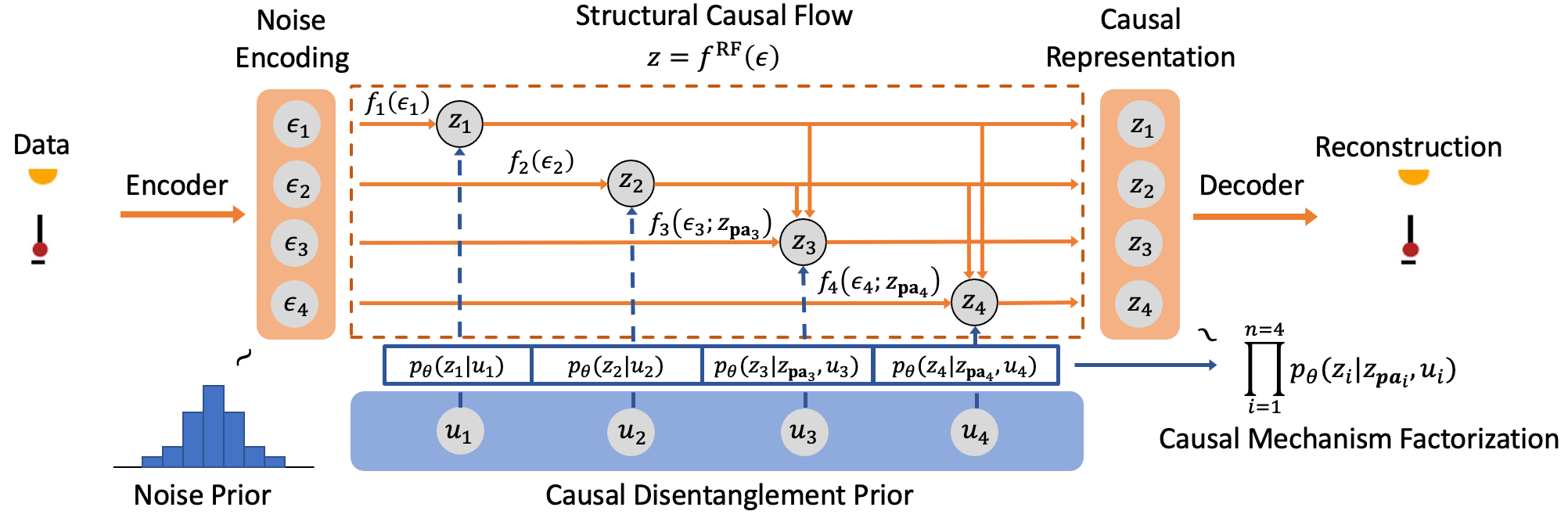
Figure 2: Architecture of ICM-VAE Framework, which contains two main components: (i) Structural Causal Flow (SCF), and (ii) Causal Disentanglement Prior.

4 Proposed Framework

We design a framework to achieve causal disentanglement. We propose ICM-VAE, a VAE-based framework based on the independent causal mechanisms (ICM) principle that achieves disentanglement of causal mechanisms. Figure 2 shows the overall architecture of our proposed framework.

Structural Causal Flow. Rather than assuming the limiting linear causal graphical model (CGM), as done in [13], we consider causal mechanisms to be complex nonlinear functions. Diverging from the strictly additive noise model assumption, we propose to parameterize causal mechanisms with a more general diffeomorphic function. Flow-based models [14] are often quite expressive in low-dimensional settings, which makes them desirable for learning complex distributions due to efficient and exact evaluation of densities. We parameterize the causal mechanisms with a conditional flow, which we refer to as the latent structural causal flow (SCF), that learns to map the independent noise distribution to a distribution over causal variables. This module is inspired by the causal autoregressive flow proposed by [15]. This type of model is more realistic and general to better capture the complex distribution over the latent causal variables compared to simple linear mappings and leads to counterfactual identifiability [16]. The SCF, denoted as $f^{\text{RF}}$, is the reduced form (RF) of a nonlinear SCM function that conceptually maps noise variables $\epsilon$ to causal variables $z$ as follows

$$z=f^{\text{RF}}(\epsilon)$$ (3)

where $f^{\text{RF}}:\mathcal{E}\to\mathcal{Z}$ is derived from the recursive substitution of causal mechanisms $f_{i}$ in topological order of the causal graph as follows

$$z_{i}=f_{i}(\epsilon_{i};z_{\textbf{pa}_{i}}),\qquad\forall i\in\{1,\dots,n\}$$ (4)

realized as a function of the noise term and parent variables. The noise encoding $\epsilon_{i}$ is exactly the SCM noise variable corresponding to the causal variable $z_{i}$.

Assuming that the causal structure is known as apriori in the form of a binary adjacency matrix obtained via an off-the-shelf causal discovery algorithm, such as the PC algorithm [17], we outline a flow-based procedure. In order to implement a diffeomorphic function $f^{\text{RF}}$, we need to ensure that it is bijective and has a differentiable inverse. Flow-based models satisfy both these requirements. Specifically, this flow is implemented as an affine autoregressive flow, where we derive each causal variable one at a time in topological order such that each variable is dependent only on a subset of previously derived variables (i.e. parents). Thus, the change of variables can be computed quite easily for exact and efficient likelihood estimation. Let’s take the pendulum example in Figure 1 to illustrate. The causal structure is $z_{1}\to z_{3},z_{4}$ and $z_{2}\to z_{3},z_{4}$. Then, the SCF would be $f^{\text{RF}}:(\epsilon_{1},\epsilon_{2},\epsilon_{3},\epsilon_{4})\mapsto(z_{1}=f_{1}(\epsilon_{1}),z_{2}=f_{2}(\epsilon_{2}),z_{3}=f_{3}(\epsilon_{3},z_{1},z_{2}),z_{4}=f_{4}(\epsilon_{4},z_{1},z_{2}))$, where $z_{i}=f^{\text{RF}}_{i}(\epsilon_{i};\epsilon_{\textbf{pa}_{i}})=f_{i}(\epsilon_{i};z_{\textbf{pa}_{i}})$ and each $f_{i}$ are affine diffeomorphic transformations of the form

$$z_{i} =f_{i}(\epsilon_{i};z_{\textbf{pa}_{i}})=\exp(a_{i})\cdot\epsilon_{i}+b_{i}$$ (5)

where $a_{i}=r_{1}(z_{\textbf{pa}_{i}})$ and $b_{i}=r_{2}(z_{\textbf{pa}_{i}})$ are the slope and offset parameters of the affine transformation, respectively, learned via neural networks $r_{1}$ and $r_{2}$ that capture information about the causal parents. Since the Jacobian of the function will be triangular by construction and the slope parameter is learned for each variable, the slope is equivalent to the diagonal elements of the Jacobian matrix as follows

$$\log\prod_{i}\bigg{|}\frac{\partial\epsilon_{i}}{\partial z_{i}}\bigg{|} =\sum_{i}\log\bigg{|}\frac{\partial f^{\text{RF}}_{i}(\epsilon_{i};\epsilon_{\textbf{pa}_{i}})}{\partial\epsilon_{i}}\bigg{|}^{-1}=\sum_{i}a_{i}$$ (6)

where $\epsilon_{\textbf{pa}_{i}}$ denotes the noise terms associated with the parents of causal variable $z_{i}$. The structural causal flow can easily be generalized to multivariate scenarios by masking groups of latent codes corresponding to each causal variable.

Generative Model. To achieve an identifiable model, we leverage auxiliary information as a weak supervision signal [11]. Let $u\in\mathbb{R}^{n}$ be the auxiliary observed labels corresponding to the causally related ground-truth factors with support $\mathcal{U}\subset\mathbb{R}^{n}$. We assume that the decoder $g$ is diffeomorphic onto its image. Several prior works [18, 11, 12], assume that the nonlinear mixing function mapping $\mathcal{Z}$ to $\mathcal{X}$ is a diffeomorphism. Consider the pendulum system from Figure 1 consisting of a light source, a pendulum, and a shadow. Given only the image, it is completely certain that we can identify where each object appears in the image. So, we find it reasonable to assume a diffeomorphic mixing function $g$ for our exploration. Let $\theta=(g,\mathbf{T},\bm{\lambda},G^{z})$ be the parameters of the conditional generative model defined as follows

$$p_{\theta}(x,\epsilon,z|u)=p_{\theta}(x|\epsilon,z)p_{\theta}(\epsilon,z|u)$$ (7)

where

$$p_{\theta}(x|\epsilon,z)=p_{\theta}(x|z)=p_{\xi}(x-g(z))$$ (8)

If we assume that the distribution over the noise $\xi$ is Gaussian with infinitesimal variance, we can model non-noisy observations as a special case of Eq. 8. The prior distribution in the generative model is given by

$$p_{\theta}(\epsilon,z|u)=p(\epsilon)p_{\theta}(z|u)$$ (9)

where we choose $p(\epsilon)$ as a standard Gaussian base distribution and $p(z|u)$ is assumed to be conditionally factorial. However, the conditional prior in Eq. (2) cannot properly capture causal mechanisms for causally related factors. We next define a causally factorized prior suitable to achieve causal disentanglement.

Causal Disentanglement Prior. We aim to use a structured prior and perform conditioning in the latent space, similar to previous work on nonlinear ICA [11], to enforce $z$ to be a disentangled causal representation. However, for a model incorporating causal structure, the form of the conditional prior in Eq. (2) needs to be modified and generalized to causally factorized distributions. To enforce the disentanglement of $z$, we parameterize the prior distribution to learn a mapping from $u$ to $z$. That is, since the goal of causal disentanglement is to map each latent/mechanism to exactly one corresponding ground-truth factor/mechanism, we can explicitly incorporate this into the prior. Using $u$ as our observational labels, we parameterize the factorized causal conditionals with a conditional flow between $u$ and $z$ to establish a bijective relationship. The goal is for the distribution over the causal variables to tend towards the learned prior. The prior over $z$ is defined as follows

$$\begin{split}p_{\theta}(z|u)&=\prod_{i=1}^{n}p_{\theta}(z_{i}|z_{\textbf{pa}_{i}},u_{i})=\prod_{i=1}^{n}p(u_{i})\bigg{|}\frac{\partial\bm{\lambda}_{i}(u_{i};z_{\textbf{pa}_{i}})}{\partial u_{i}}\bigg{|}^{-1}\end{split}$$ (10)

$$\begin{split}p_{\theta}(z_{i}|z_{\textbf{pa}_{i}},u_{i})=h_{i}(z_{i})\exp(\mathbf{T}_{i}(z_{i}|z_{\textbf{pa}_{i}})\bm{\lambda}_{i}(G_{i}^{z}\odot z,u_{i})-\psi_{i}(z,u))\end{split}$$ (11)

where $\bm{\lambda}_{i}(G_{i}^{z}\odot z,u_{i})$ is the estimated parameter vector of the prior obtained via mechanism $\bm{\lambda}_{i}$, $G^{z}_{i}$ is the $i$th column of the adjacency matrix of the causal graph of $z$, $h_{i}(z)$ is the base measure, and $\mathbf{T}_{i}(z)=(z,z^{2})$ is the sufficient statistic. The prior induces a causal factorization of $z$ with causal conditionals $p_{\theta}(z_{i}|z_{\textbf{pa}_{i}},u_{i})$, where $u_{i}$ is introduced as a weak supervision signal for identifiability. Eq. (10) is reminiscent of temporal priors that define a distribution over a latent variable conditioned on the variable at a previous time step [19]. In our case, we view the causal factors as derived autoregressively. With a slight abuse of notation, we define $\bm{\lambda}(z,u)$ to be the concatenation of all $\bm{\lambda}_{i}(G_{i}^{z}\odot z,u_{i})$. The function $\bm{\lambda}(z,u)$ outputs the natural parameter vector for the causally factorized distribution. We further require $\bm{\lambda}:\mathcal{Z}\times\mathcal{U}\to\mathcal{Z}$ to learn a bijective map between $u$ and learned representation $z$ to encourage disentanglement of the causal mechanisms. In practice, we choose $p(u)$ from a location-scale family such as Gaussian. The mechanism $\bm{\lambda}_{i}$ is defined as the following diffeomorphic map:

$$\bm{\lambda}_{i} (u_{i};z_{\textbf{pa}_{i}})=\exp(c_{i})\cdot u_{i}+d_{i}$$ (12)

where $c_{i}=s_{1}(z_{\textbf{pa}_{i}})$ and $d_{i}=s_{2}(z_{\textbf{pa}_{i}})$ are the slope and offset parameters of the flow, respectively, learned via neural networks. To obtain a causally factorized conditional prior over $z$, we map the base distribution $p(u)$, which is known beforehand, to a distribution over $z$.

Learning Objective. Putting all the components together, ICM-VAE consists of a stochastic encoder $q_{\phi}(\epsilon,z|x,u)$, a decoder $p_{\theta}(x|\epsilon,z)$, and diffeomorphic causal transformations $f_{i}(\cdot;\epsilon)$. All components are learnable and implemented as neural networks. Formally, we optimize the following variational lower bound:

$$\begin{split}\log p_{\theta}(x,u)\geq\mathbb{E}_{\epsilon,z\sim q_{\phi}(\epsilon,z|x,u)}\Big{[}\log p_{\theta}(x|\epsilon)+\log p_{\theta}(x|z)&-\beta\{\log q_{\phi}(\epsilon|x,u)+\log q_{\phi}(z|x,u)\\ &-\log p(\epsilon)-\log p_{\theta}(z|u)\}\Big{]}\end{split}$$ (13)

where $\beta$ is the latent bottleneck parameter. We train the model by minimizing the negative of the ELBO loss and learn to map low-level pixel data to noise variables and map the noise variable distribution to a distribution over the causal variables. For a detailed derivation of the ELBO, see Appendix B.3.

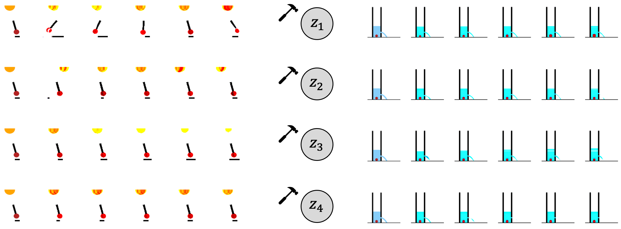
Figure 3: (Pendulum and Flow) Counterfactually generated images after intervening on causal factor $z_{1}$, $z_{2}$, $z_{3}$, and $z_{4}$, individually, and propagating causal effects.

5 Identifiability Analysis

The causally factorized prior in Eq. (10) induces disentanglement of causal mechanisms. Theorem 1 extends the identifiability theorem of [11] to show causal mechanism equivalence identifiability when we have a causal model. We note that the causal mechanism disentanglement implies the disentanglement of causal factors. For a full proof of Theorem 1, see Appendix B.1.

Theorem 1 (Identifiability of ICM-VAE).

Suppose that we observe data sampled from a generative model defined according to (7)-(11) with two sets of model parameters $\theta=(g,\mathbf{T},\bm{\lambda},G^{z})$ and $\hat{\theta}=(\hat{g},\hat{\mathbf{T}},\hat{\bm{\lambda}},\hat{G}^{z})$. Suppose the following assumptions hold

1. The set $\{x\in\mathcal{X}|\phi_{\xi}(x)=0\}$ has measure zero, where $\phi_{\xi}$ is the characteristic function of the density $p_{\xi}$ defined in Eq. (8).

2. The decoder $g$ is diffeomorphic onto its image.

3. The sufficient statistics $\mathbf{T}_{i}$ are diffeomorphic.

4. [Sufficient Variability] There exists $nk+1$ distinct points $u_{0},\dots,u_{nk}$ such that the matrix

   $$L=(\bm{\lambda}(z_{\textbf{pa}_{(1)}},u_{(1)})-\bm{\lambda}(z_{(0)},u_{(0)}),\dots,\bm{\lambda}(z_{\textbf{pa}_{(nk)}},u_{(nk)})-\bm{\lambda}(z_{(0)},u_{(0)}))$$ (14)

   of size $nk\times nk$ is invertible, the ground-truth function $\bm{\lambda}$ is affected sufficiently strongly by each individual label $u_{i}$ and previously derived variables $z_{\textbf{pa}_{i}}$, and $\forall i$, $\bm{\lambda}_{i}(z_{\textbf{pa}_{i}},u_{i})\neq 0$.

Then $\theta$ and $\hat{\theta}$ are causal mechanism permutation-equivalent, and the model $\hat{\theta}$ is causally disentangled.

Table 1: Causal Disentanglement

Dataset	Model	$D$	$C$	IRS
Pendulum	$\beta$-VAE	$0.182$	$0.285$	$0.449$
	iVAE	$0.483$	$0.385$	$0.670$
	CausalVAE	$0.885$	$0.539$	$0.817$
	SCM-VAE	$0.764$	$0.475$	$0.829$
	ICM-VAE (Ours)	$\mathbf{0.997}$	$\mathbf{0.882}$	$\mathbf{0.869}$
Flow	$\beta$-VAE	$0.308$	$0.332$	$0.452$
	iVAE	$0.730$	$0.481$	$0.674$
	CausalVAE	$0.819$	$0.522$	$0.707$
	SCM-VAE	$0.854$	$0.483$	$0.811$
	ICM-VAE (Ours)	$\mathbf{0.988}$	$\mathbf{0.598}$	$\mathbf{0.893}$
CausalCircuit	$\beta$-VAE	$0.692$	$0.442$	$0.982$
	iVAE	$0.745$	$0.541$	$0.992$
	CausalVAE	$0.886$	$0.625$	$0.994$
	SCM-VAE	$0.867$	$0.652$	$0.993$
	ICM-VAE (Ours)	$\mathbf{0.982}$	$\mathbf{0.689}$	$\mathbf{0.999}$

6 Experimental Evaluation

We run experiments on the Pendulum, Flow, and CausalCircuit datasets, each consisting of four continuous-valued causal variables, and evaluate disentanglement, completeness, interventional robustness, and counterfactual generation.

Discussion. Our experiments show that learning diffeomorphic causal mechanisms and incorporating the causal structure to learn a bijective $\bm{\lambda}$ to estimate the parameters of the causally factorized distribution significantly improves the disentanglement and interventional robustness of learned causal factors compared with baselines, as shown in Table 1. Consistent with our intuition, iVAE fails to disentangle the causal factors. The results indicate that ICM-VAE disentangles the causal factors and mechanisms almost perfectly. A high DCI disentanglement score indicates a permutation matrix mapping the latent factors to ground-truth generative factors in an ideal one-to-one mapping [20, 21]. Further, our model improves the interventional robustness [22] of the representation, where interventions on ground-truth factors map to interventions on the corresponding learned factors. We also show counterfactually generated results of intervening on learned latent factors. Figure 4 shows the CausalCircuit system and the result of intervening on the robot arm factor and propagating causal effects. We observe that the red light also turns on as the robot arm interacts with the blue or green lights. On the other hand, when the arm interacts with the red light, only the red light turns on and the other lights remain off. We observe a similar phenomenon in the Pendulum and Water Flow systems in Figure 3. Our code is available at https://github.com/Akomand/ICM-VAE.

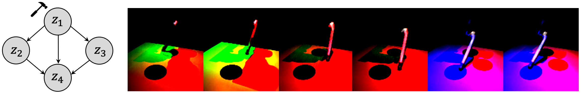
Figure 4: (CausalCircuit) Counterfactually generated samples as a result of intervening on $z_{1}$. Observe that the robot arm moves and turns on the blue, green, or red lights, which causally affect other lights.

7 Conclusion

In this work, we propose a framework for causal representation learning under supervision from labels. We model causal mechanisms as learned flow-based diffeomorphic transformations from noise to causal variables. We propose the notion of causal mechanism disentanglement for causal models and a causal disentanglement prior, which causally factorizes the learned distribution over causal variables. We also theoretically show the identifiability of the learned causal factors up to permutation and elementwise reparameterization. We experimentally validate our method and show that our model almost perfectly disentangles the causal factors, improves interventional robustness, and generates consistent counterfactual instances. We focus on causally disentangled representations with a known causal structure. Future work includes incorporating causal discovery methods when the causal graph is unknown and exploring identifiability results given only partially observed labels.

8 Acknowledgements

This work is supported in part by National Science Foundation under awards 1910284, 1946391 and 2147375, the National Institute of General Medical Sciences of National Institutes of Health under award P20GM139768, and the Arkansas Integrative Metabolic Research Center at University of Arkansas.

Appendices

Appendix A Background

Structural Causal Model. In this work, we assume $z$ is described by a structural causal model (SCM), which is formally defined by a tuple $\mathcal{M}=\langle\mathcal{Z},\mathcal{E},F\rangle$, where $\mathcal{Z}$ is the domain of the set of $n$ endogenous causal variables $z=\{z_{1},\dots,z_{n}\}$, $\mathcal{E}$ is the domain of the set of $n$ exogenous noise variables $\epsilon=\{\epsilon_{1},\dots,\epsilon_{n}\}$, which is learned as an intermediate latent variable, and $F=\{f_{1},\dots,f_{n}\}$ is a collection of $n$ independent causal mechanisms of the form

$$z_{i}=f_{i}(\epsilon_{i},z_{\textbf{pa}_{i}})$$ (15)

where $\forall i$, $f_{i}:\mathcal{E}_{i}\times\prod_{j\in\textbf{pa}_{i}}\mathcal{Z}_{j}\to\mathcal{Z}_{i}$ are causal mechanisms that determine each causal variable as a function of the parents and noise, $z_{\textbf{pa}_{i}}$ are the parents of causal variable $z_{i}$; and a probability measure $p_{\mathcal{E}}(\epsilon)=p_{\mathcal{E}_{1}}(\epsilon_{1})p_{\mathcal{E}_{2}}(\epsilon_{2})\dots p_{\mathcal{E}_{n}}(\epsilon_{n})$, which admits a product distribution. An SCM where the exogenous noise variables are jointly independent (no hidden confounders) is known as a Markovian model, which is the setting we assume for the purposes of this work. We depict the causal structure of $z$ by a causal directed acyclic graph (DAG) $\mathcal{G}^{z}$ with adjacency matrix $G^{z}\in\{0,1\}^{n\times n}$.

Appendix B Theory

B.1 Restatement and Proof of Theorem 1

Definition 7 (Minimal Sufficient Statistic [12]).

Given a parameterized distribution in the exponential family, we say its sufficient statistic $\mathbf{T}_{i}$ is minimal when there exists no $v\neq 0$ such that $v^{T}\mathbf{T}_{i}(z)$ is constant for all $z\in\mathcal{Z}$.

Definition 8 (Permutation-Scaling Matrix [12]).

A matrix is permutation-scaling if every row or column contains exactly one non-zero element.

Lemma 1 ([12]).

A sufficient statistic $\mathbf{T}:\mathcal{Z}\to\mathbb{R}^{k}$ is minimal if and only if there exist $z_{(0)},\dots,z_{(k)}$ belonging to the support of $\mathcal{Z}$ such that the following $k$-dimensional vectors are linearly independent:

$$\mathbf{T}(z_{(1)})-\mathbf{T}(z_{(0)}),\dots,\mathbf{T}(z_{(k)})-\mathbf{T}(z_{(0)})$$ (16)

Definition 9.

A conditional sufficient statistic $\mathbf{T}(z|y):\mathcal{Z}\times\mathcal{Y}\to\mathbb{R}^{k}$ describes the sufficient statistics of the conditional distribution of $z$ induced as a result of conditioning on variable $y$.

Definition 10.

For all $i,j\in\{1,\dots,n\}$, if $\mathbf{T}_{i}(z_{i}|z_{\textbf{pa}_{i}})$ and $\hat{\mathbf{T}}_{i}(z_{j}|z_{\textbf{pa}_{j}})$ are causal permutation-equivalent, then $z_{i}$ and $z_{j}$ are permutation-equivalent.

We adapt the theory from [12] and [11] and propose the following theorem for identifiability.

Theorem 1 (Identifiability of ICM-VAE).

Suppose that we observe data sampled from a generative model defined according to (7)-(11) with two sets of model parameters $\theta=(g,\mathbf{T},\bm{\lambda},G^{z})$ and $\hat{\theta}=(\hat{g},\hat{\mathbf{T}},\hat{\bm{\lambda}},\hat{G}^{z})$. Suppose the following assumptions hold

1. The set $\{x\in\mathcal{X}|\phi_{\xi}(x)=0\}$ has measure zero, where $\phi_{\xi}$ is the characteristic function of the density $p_{\xi}$ defined in Eq. (8).

2. The decoder $g$ is diffeomorphic onto its image.

3. The sufficient statistics $\mathbf{T}_{i}$ are diffeomorphic.

4. [Sufficient Variability] There exists $nk+1$ distinct points $u_{0},\dots,u_{nk}$ such that the matrix

   $$L=(\bm{\lambda}(z_{\textbf{pa}_{(1)}},u_{(1)})-\bm{\lambda}(z_{(0)},u_{(0)}),\dots,\bm{\lambda}(z_{\textbf{pa}_{(nk)}},u_{(nk)})-\bm{\lambda}(z_{(0)},u_{(0)}))$$ (17)

   of size $nk\times nk$ is invertible, the ground-truth function $\bm{\lambda}$ is affected sufficiently strongly by each individual label $u_{i}$ and previously derived variables $z_{\textbf{pa}_{i}}$, and $\forall i$, $\bm{\lambda}_{i}(z_{\textbf{pa}_{i}},u_{i})\neq 0$.

Then $\theta$ and $\hat{\theta}$ are causal mechanism permutation-equivalent, and the model $\hat{\theta}$ is causally disentangled.

Proof.

In order to show that the set of parameters $\hat{\theta}$ is identifiable up to permutation, we break down the proof into five main steps.

Step 1 (Equality of Denoised Distributions). Firstly, we show that we can transform the equality of observed data distributions into a statement about the equality of noiseless distributions. Suppose we have two sets of parameters $\theta$ and $\hat{\theta}$ such that their marginal distributions are equivalent as follows:

$$p_{\theta}(x|u)=p_{\hat{\theta}}(x|u)$$ (18)

for all pairs $(x,u)$. Let $g^{-1}=s\circ a^{-1}$ be the encoding of causal factors $z$, where $a^{-1}$ is the encoding of the noise variables $\epsilon$. Then, we have the following

$$\int_{\mathcal{Z}}p_{\mathbf{T},\bm{\lambda}}(z|u)p_{g}(x|z)\;dz =\int_{\mathcal{Z}}p_{\hat{\mathbf{T}},\hat{\bm{\lambda}}}(z|u)p_{\hat{g}}(x|z)\;dz$$ (19)

$$\int_{\mathcal{Z}}p_{\mathbf{T},\bm{\lambda}}(z|u)p_{\xi}(x-g(z))\;dz =\int_{\mathcal{Z}}p_{\hat{\mathbf{T}},\hat{\bm{\lambda}}}(z|u)p_{\xi}(x-\hat{g}(x))\;dz$$ (20)

$$\int_{\mathcal{X}}p_{\mathbf{T},\bm{\lambda}}(g^{-1}(\bar{x})|u)\det J_{g^{-1}}(\bar{x})p_{\xi}(x-\bar{x})\;d\bar{x} =\int_{\mathcal{X}}p_{\hat{\mathbf{T}},\hat{\bm{\lambda}}}(\hat{g}^{-1}(\bar{x})|u)\det J_{\hat{g}^{-1}}(\bar{x})p_{\xi}(x-\bar{x})\;d\bar{x}$$ (21)

$$\int_{\mathbb{R}^{d}}p_{\mathbf{T},\bm{\lambda},g,u}(\bar{x})p_{\xi}(x-\bar{x})\;d\bar{x} =\int_{\mathbb{R}^{d}}p_{\hat{\mathbf{T}},\hat{\bm{\lambda}},\hat{g},\hat{u}}(\bar{x})p_{\xi}(x-\bar{x})\;d\bar{x}$$ (22)

$$(p_{\mathbf{T},\bm{\lambda},g,u}*p_{\xi})(x) =(p_{\hat{\mathbf{T}},\hat{\bm{\lambda}},\hat{g},\hat{u}}*p_{\xi})(x)$$ (23)

$$\mathcal{F}[p_{\mathbf{T},\bm{\lambda},g,u}](w)\phi_{\xi}(w) =\mathcal{F}[p_{\hat{\mathbf{T}},\hat{\bm{\lambda}},\hat{g},\hat{u}}](w)\phi_{\xi}(w)$$ (24)

$$\mathcal{F}[p_{\mathbf{T},\bm{\lambda},g,u}](w) =\mathcal{F}[p_{\hat{\mathbf{T}},\hat{\bm{\lambda}},\hat{g},\hat{u}}](w)$$ (25)

$$p_{\mathbf{T},\bm{\lambda},g,u} =p_{\hat{\mathbf{T}},\hat{\bm{\lambda}},\hat{g},\hat{u}}$$ (26)

where $\mathcal{F}$ is the Fourier transform. Eq. (24) and Eq. (26) use the fact that the Fourier transform is invertible and Eq. (25) is an application of the fact that the Fourier transform of a convolution is the product of their Fourier transforms. Thus, we have shown that if the distributions with added noise are the same, then the noise-free distributions must also be the same over all possible values $(x,u)$ within the support.

Step 2 (Linear relationship). Define $v=\hat{g}^{-1}\circ g:\mathcal{Z}\to\hat{\mathcal{Z}}$. By replacing Eq. (26) with the exponential form of the conditional prior from Eq. (10), we obtain the following:

$$p_{\mathbf{T},\bm{\lambda}}(z|u) =p_{\hat{\mathbf{T}},\hat{\bm{\lambda}}}(z|u)$$ (27)

$$p_{\mathbf{T},\bm{\lambda}}(g^{-1}(x)|u)\det J_{g^{-1}}(x) =p_{\hat{\mathbf{T}},\hat{\bm{\lambda}}}(\hat{g}^{-1}(x)|u)\det J_{\hat{g}^{-1}}(x)$$ (28)

$$\begin{split}&\prod_{i=1}^{n}h_{i}(g^{-1}_{i}(x))\exp\Bigg{[}\sum_{j=1}^{k}T_{i,j}(g^{-1}_{i}(x)|g^{-1}_{\textbf{pa}_{i}}(x))\lambda_{i,j}(z_{\textbf{pa}_{i}},u_{i})-\psi_{i}(z_{\textbf{pa}_{i}},u_{i})\Bigg{]}\det J_{g^{-1}}(x)=\\ &\prod_{i=1}^{n}h_{i}(\hat{g}^{-1}_{i}(x))\exp\Bigg{[}\sum_{j=1}^{k}\hat{T}_{i,j}(\hat{g}^{-1}_{i}(x)|g^{-1}_{\textbf{pa}_{i}}(x))\hat{\lambda}_{i,j}(v(z_{\textbf{pa}_{i}}),u_{i})-\hat{\psi}_{i}(z_{\textbf{pa}_{i}},u_{i})\Bigg{]}\det J_{\hat{g}^{-1}}(x)\end{split}$$ (29)

Taking the logarithm of both sides of Eq. (29) yields the following

$$\begin{split}\log\det J_{g^{-1}}(x)&+\sum_{i=1}^{n}\log h_{i}(g^{-1}_{i}(x))+\sum_{j=1}^{k}T_{i,j}(g_{i}^{-1}(x)|g^{-1}_{\textbf{pa}_{i}}(x))\lambda_{i,j}(z_{\textbf{pa}_{i}},u)-\psi_{i}(z_{\textbf{pa}_{i}},u_{i})\\ &=\log\det J_{\hat{g}^{-1}}(x)+\sum_{i=1}^{n}\log\hat{h}_{i}(\hat{g}^{-1}_{i}(x))+\sum_{j=1}^{k}\hat{T}_{i,j}(\hat{g}_{i}^{-1}(x)|g^{-1}_{\textbf{pa}_{i}}(x))\hat{\lambda}_{i,j}(v(z_{\textbf{pa}_{i}}),u)\\ &-\hat{\psi}_{i}(z_{\textbf{pa}_{i}},u_{i})\end{split}$$ (30)

Let $u_{0},\dots,u_{nk}$ be the points provided by assumption 4 and define $\Delta\bm{\lambda}(z_{\textbf{pa}},u)=\bm{\lambda}(z_{\textbf{pa}},u)-\bm{\lambda}(z_{0},u_{0})$. The notation $z_{\textbf{pa}}$ indicates that each causal variable in $z$ is derived from its parents. We substitute each of the $u_{\ell}$ in the above equation to obtain $nk+1$ distinct equations. Using $u_{0}$ as a pivot, we subtract the first equation for $u_{0}$ from the remaining $nk$ equations to obtain

$$\begin{split}\forall\ell\in 1,\dots,nk,\;\qquad\mathbf{T}(g^{-1}(x))^{T}&\Delta\bm{\lambda}(z_{\textbf{pa}_{\ell}},u_{\ell})-\sum_{i}\psi_{i}(z_{\textbf{pa}_{\ell}},u_{\ell})-\psi_{i}(z_{0},u_{0})\\ =&\hat{\mathbf{T}}(\hat{g}^{-1}(x))^{T}\Delta\hat{\bm{\lambda}}(v(z_{\textbf{pa}_{\ell}}),u_{\ell})-\sum_{i}\hat{\psi}_{i}(z_{\textbf{pa}_{\ell}},u_{\ell})-\hat{\psi}_{i}(z_{0},u_{0})\end{split}$$ (31)

Now, let $L$ be the full-rank matrix described in the sufficient variability assumption (assumption 4), and $\hat{L}$ the matrix defined with respect to $\hat{\bm{\lambda}}$. Note that $\hat{L}$ is not guaranteed to be full-rank. Regrouping all normalizing constants $\psi$ into a term $b_{\ell}=d(z_{\textbf{pa}_{\ell}},z_{0},u_{\ell},u_{0})$ and letting $b$ be the vector of all $b_{\ell}$ for all $\ell\in\{1,\dots,nk\}$, we obtain the following:

$$L^{T}\mathbf{T}(g^{-1}(x))=\hat{L}^{T}\hat{\mathbf{T}}(\hat{g}^{-1}(x))+b$$ (32)

Since $L$ is assumed to be invertible, we can multiply by the inverse of $L^{T}$ on both sides to obtain the following

$$\mathbf{T}(g^{-1}(x))=A\hat{\mathbf{T}}(\hat{g}^{-1}(x))+c$$ (33)

where $A=(L^{T})^{-1}\hat{L}$ and $c=(L^{T})^{-1}b$.

Step 3 (Invertibility of $A$). We show that $A$ is an invertible matrix. By Lemma 1, we have that the minimality of sufficient statistic $\mathbf{T}_{i}$ implies that the following set of vectors is linearly independent:

$$\mathbf{T}_{i}(z_{i}^{(1)})-\mathbf{T}_{i}(z_{i}^{(0)}),\dots,\mathbf{T}_{i}(z_{i}^{(k)})-\mathbf{T}_{i}(z_{i}^{(0)})$$ (34)

Define

$$z^{(0)}=[z_{1}^{(0)},\dots,z_{n}^{(0)}]^{T}\in\mathbb{R}^{n}$$ (35)

For all $i\in\{1,\dots,n\}$ and $p\in\{1,\dots,k\}$, define the vectors

$$z^{(p,i)}=[z_{1}^{(0)},\dots,z_{i-1}^{(0)},z_{i}^{(p)},z_{i+1}^{(0)}\dots,z_{n}^{(0)}]^{T}\in\mathbb{R}^{n}$$ (36)

Now, for $1\leq p\leq k$ and $i\in\{1,\dots,n\}$, we consider the following difference

$$\mathbf{T}(z^{(p,i)})-\mathbf{T}(z^{(0)})=A[\hat{\mathbf{T}}(z^{(p,i)})-\hat{\mathbf{T}}(z^{(0)})]$$ (37)

where the LHS is a vector filled with zeros except for the block corresponding to $\mathbf{T}_{i}(z_{i}^{(p,i)})-\mathbf{T}(z_{i}^{(0)})$. Define

$$\Delta\mathbf{T}^{(i)}=[\mathbf{T}(z^{(1,i)})-\mathbf{T}(z^{(0)})\dots\mathbf{T}(z^{(k,i)})-\mathbf{T}(z^{(0)})]$$ (38)

and

$$\Delta\hat{\mathbf{T}}^{(i)}=[\hat{\mathbf{T}}(z^{(1,i)})-\hat{\mathbf{T}}(z^{(0)})\dots\hat{\mathbf{T}}(z^{(k,i)})-\hat{\mathbf{T}}(z^{(0)})]$$ (39)

Then, we have that the columns of both these are linearly independent and all rows are filled with zeros except the block of rows $\{(i-1)k+1,\dots,ik\}$. So, writing Eq. (37) in matrix form and grouping all components, we have the following

$$[\Delta\mathbf{T}^{(1)},\dots,\Delta\mathbf{T}^{(n)}]=A[\Delta\hat{\mathbf{T}}^{(1)},\dots,\Delta\hat{\mathbf{T}}^{(n)}]$$ (40)

Thus, we have a block diagonal matrix of size $nk\times nk$. Since each block is invertible, $[\Delta\mathbf{T}^{(1)},\dots,\Delta\mathbf{T}^{(n)}]$ must be invertible. This implies that $A$ must be invertible. Thus, Eq. (33) and the invertibility of $A$ imply that $\theta\sim_{A}\hat{\theta}$.

Step 4 (Linear relationship of natural parameters). In addition to showing the linear relationship between the sufficient statistic, we also show the linear relationship linking $\bm{\lambda}$ and $\hat{\bm{\lambda}}$. Define $v=\hat{g}^{-1}\circ g:\mathcal{Z}\to\hat{\mathcal{Z}}$. That is, there exists a diffeomorphism between the learned and ground-truth factors. We rewrite Eq. (30) as follows:

$$\mathbf{T}(g^{-1}(x))^{T}\bm{\lambda}(z_{\textbf{pa}},u)=\hat{\mathbf{T}}(\hat{g}^{-1}(x))^{T}\hat{\bm{\lambda}}(v(z_{\textbf{pa}}),u)+\kappa(z_{\textbf{pa}},u)+\gamma(z)$$ (41)

where we combine all terms depending only on $z$ into $\gamma$ and those depending only on $u$ into $\kappa$. Now, we can rewrite the above as follows using the linear relationship between sufficient statistics:

$$\hat{\mathbf{T}}(\hat{g}^{-1}(x))^{T}A^{T}\bm{\lambda}(z_{\textbf{pa}},u)+c^{T}\bm{\lambda}(z_{\textbf{pa}},u)=\hat{\mathbf{T}}(\hat{g}^{-1}(x))^{T}\hat{\bm{\lambda}}(v(z_{\textbf{pa}}),u)+\kappa(z_{\textbf{pa}},u)+\gamma(z)$$ (42)

$$\hat{\mathbf{T}}(\hat{g}^{-1}(x))^{T}A^{T}\bm{\lambda}(z_{\textbf{pa}},u)=\hat{\mathbf{T}}(\hat{g}^{-1}(x))^{T}\hat{\bm{\lambda}}(v(z_{\textbf{pa}}),u)+\bar{\kappa}(z_{\textbf{pa}},u)+\gamma(z)$$ (43)

where $\bar{\kappa}$ absorbs all $u$-dependent terms. We can simplify this equality to the following:

$$\hat{\mathbf{T}}(\hat{g}^{-1}(x))^{T}(A^{T}\bm{\lambda}(z_{\textbf{pa}},u)-\hat{\bm{\lambda}}(v(z_{\textbf{pa}}),u))=\bar{\kappa}(z_{\textbf{pa}},u)+\gamma(z)$$ (44)

$$\mathbf{T}(\hat{g}^{-1}(x))^{T}(A^{T}\bm{\lambda}(z_{\textbf{pa}},u)-\hat{\bm{\lambda}}(v(z_{\textbf{pa}}),u))=\bar{\kappa}(z_{\textbf{pa}},u)+\gamma(\hat{g}^{-1}(x))$$ (45)

Taking the finite difference between distinct values $z$ and $\bar{z}$ yields

$$[\mathbf{T}(z)-\mathbf{T}(\bar{z})]^{T}(A^{T}\bm{\lambda}(z_{\textbf{pa}},u)-\hat{\bm{\lambda}}(v(z_{\textbf{pa}}),u))=\gamma(\hat{g}^{-1}(x))-\gamma(\hat{g}^{-1}(\bar{x}))$$ (46)

Now, we can construct an invertible matrix $[\Delta\mathbf{T}^{(1)}\dots\Delta\mathbf{T}^{(n)}]$ such that

$$[\Delta\mathbf{T}^{(1)}\dots\Delta\mathbf{T}^{(n)}]^{T}(A^{T}\bm{\lambda}(z_{\textbf{pa}},u)-\hat{\bm{\lambda}}(v(z_{\textbf{pa}}),u))=[\Delta\gamma^{(1)}\dots\Delta\gamma^{(n)}]$$ (47)

Due to this invertibility, we can simplify the above to obtain

$$A^{T}\bm{\lambda}(z_{\textbf{pa}},u)+\gamma=\hat{\bm{\lambda}}(v(z_{\textbf{pa}}),u)$$ (48)

where

$$\gamma=-[\Delta\mathbf{T}^{(1)}\dots\Delta\mathbf{T}^{(n)}]^{-T}[\Delta\gamma^{(1)}\dots\Delta\gamma^{(n)}]$$ (49)

We can rewrite this as follows to yield the equivalence of $\bm{\lambda}$ and $\hat{\bm{\lambda}}$

$$A^{T}\bm{\lambda}(z_{\textbf{pa}},u)+\gamma=\hat{\bm{\lambda}}(v(z_{\textbf{pa}}),u)$$ (50)

Step 5 (Permutation Equivalence). To show that $A$ is a permutation-scaling matrix, we have to show that any two columns cannot have nonzero entries on the same row.

• If $G^{z}$ is fixed, we are done since the trivial permutation always holds. Since the decoder is assumed to be diffeomorphic, there is a point-wise nonlinearity between each corresponding factor of the representation. Thus, a bijective mapping establishes a component-wise reparameterization (scaling) and trivial permutation.

• If $G^{z}$ is learned, then for a learned sparse graph $\hat{G}^{z}$ if the following holds

  $$\pi(\hat{G}^{z})=G^{z}$$ (51)

  then we still achieve permutation equivalence by permuting the causal graph.

We conclude that $A$ must be a causal permutation-scaling matrix. Since $\bm{\lambda}$ captures the causal dependencies between factors of $z$, we have that the following must be true

$$\mathbf{T}_{i}(z_{i}|z_{\textbf{pa}_{i}})=A_{ij}\hat{\mathbf{T}}_{j}(z_{j}|z_{\textbf{pa}_{j}})$$ (52)

Thus, $\mathbf{T}$, $\hat{\mathbf{T}}$ and $\bm{\lambda}$, $\hat{\bm{\lambda}}$ must be causal mechanism permutation-equivalent, respectively, and $z$ is causally disentangled. Therefore, $z$ is disentangled, and we have that $\theta\sim_{P}\hat{\theta}$, where $P=A$ is a permutation-scaling matrix.

B.2 Traditional disentanglement cannot guarantee independent causal mechanisms equivalence

In this section, we provide a counterexample to show that the traditional notion of disentanglement cannot capture the equivalence of causal mechanisms. For example, consider the running example of the Pendulum system. We have four causal factors that are causally related. Let $z$ denote the true factors of variation and $\hat{z}$ denote the learned factors, where each $z_{i}$ and $\hat{z}_{i}$ correspond to the same causal variable. For the sake of simplicity, suppose we have a linear SCM:

Ground-truth SCM

$$\vbox{\hbox{\includegraphics[scale={0.5}]{images/true_factors.png}}}\qquad\qquad\begin{aligned} z_{1}&=\epsilon_{1}\sim\mathcal{N}(0,1)\\ z_{2}&=\epsilon_{2}\sim\mathcal{N}(0,1)\\ z_{3}&=az_{1}+bz_{2}+\epsilon_{3}\\ z_{4}&=cz_{1}+dz_{2}+\epsilon_{4}\end{aligned}$$

Learned SCM

$$\vbox{\hbox{\includegraphics[scale={0.5}]{images/learned_factors.png}}}\qquad\qquad\begin{aligned} \hat{z}_{1}&=\hat{\epsilon}_{1}\sim\mathcal{N}(0,1)\\ \hat{z}_{2}&=\hat{\epsilon}_{2}\sim\mathcal{N}(0,1)\\ \hat{z}_{3}&=b\hat{z}_{1}+a\hat{z}_{2}+\hat{\epsilon}_{3}\\ \hat{z}_{4}&=d\hat{z}_{1}+c\hat{z}_{2}+\hat{\epsilon}_{4}\end{aligned}$$

Marginal

$$\begin{aligned} z_{1}&\sim\mathcal{N}(0,1)\\ z_{2}&\sim\mathcal{N}(0,1)\\ z_{3}&\sim\mathcal{N}(0,\sqrt{a^{2}+b^{2}+1^{2}})\\ z_{4}&\sim\mathcal{N}(0,\sqrt{c^{2}+d^{2}+1^{2}})\end{aligned}\qquad\qquad\begin{aligned} \hat{z}_{1}&\sim\mathcal{N}(0,1)\\ \hat{z}_{2}&\sim\mathcal{N}(0,1)\\ \hat{z}_{3}&\sim\mathcal{N}(0,\sqrt{b^{2}+a^{2}+1^{2}})\\ \hat{z}_{4}&\sim\mathcal{N}(0,\sqrt{d^{2}+c^{2}+1^{2}})\end{aligned}$$

Observe that the causal mechanisms learned are different than the true causal mechanisms. In the linear case, for simplicity, we swap the coefficients. We have the following equivalent marginal distribution for true and learned factors:

$$p(z)=p(z_{1})p(z_{2})p(z_{3}|z_{1},z_{2})p(z_{4}|z_{1},z_{2})\approx p(\hat{z}_{1})p(\hat{z}_{2})p(\hat{z}_{3}|\hat{z}_{1},\hat{z}_{2})p(\hat{z}_{4}|\hat{z}_{1},\hat{z}_{2})=p(\hat{z})$$

However, traditional disentanglement does not imply an equivalence of all the individual causal mechanisms of the true and learned factors. In the above example, the true SCM consists of different mechanisms than the learned SCM, but both yield the same marginal distribution. This example violates the causal mechanism permutation equivalence and causal disentanglement but satisfies traditional disentanglement. We claim that learning a model that achieves equivalence of causal mechanisms from the perspective of the ICM principle better captures disentanglement in the causal setting.

B.3 Derivation of ICM-VAE ELBO

We aim to push the variational posterior distribution $q_{\phi}(\epsilon,z|x,u)$ to the true joint posterior distribution $p_{\theta}(\epsilon,z|x,u)$. Formally, the goal is to minimize the KL divergence as follows:

$\mathcal{D}(q_{\phi}(\epsilon,z|x,u),p_{\theta}(\epsilon,z|x,u))=$

$$\int\int q_{\phi}(\epsilon,z|x,u)\log\frac{q_{\phi}(\epsilon,z|x,u)}{p_{\theta}(\epsilon,z|x,u)}\;d\epsilon\;dz$$ (53)

$$=\int\int q_{\phi}(\epsilon,z|x,u)\log\frac{q_{\phi}(\epsilon,z|x,u)p_{\theta}(x,u)}{p_{\theta}(\epsilon,z,u,x)}\;d\epsilon\;dz$$ (54)

$$=\int\int q_{\phi}(\epsilon,z|x,u)\Big{[}\log p_{\theta}(x,u)+\log\frac{q_{\phi}(\epsilon,z|x,u)}{p_{\theta}(\epsilon,z,u,x)}\Big{]}\;d\epsilon\;dz$$ (55)

$$=\int\int q_{\phi}(\epsilon,z|x,u)\log p_{\theta}(x,u)+q_{\phi}(\epsilon,z|x,u)\log\frac{q_{\phi}(\epsilon,z|x,u)}{p_{\theta}(\epsilon,z,u,x)}\;d\epsilon\;dz$$ (56)

$$=\log p_{\theta}(x,u)+\int\int q_{\phi}(\epsilon,z|x,u)\log\frac{q_{\phi}(\epsilon,z|x,u)}{p_{\theta}(\epsilon,z,u,x)}\;d\epsilon\;dz$$ (57)

$$=\log p_{\theta}(x,u)+\int\int q_{\phi}(\epsilon,z|x,u)\log\frac{q_{\phi}(\epsilon,z|x,u)}{p_{\theta}(x|\epsilon,z,u)p_{\theta}(\epsilon,z,u)}\;d\epsilon\;dz$$ (58)

$$=\log p_{\theta}(x,u)+\mathbb{E}_{\epsilon,z\sim q_{\phi}(\epsilon,z|x,u)}\Big{[}\log\frac{q_{\phi}(\epsilon,z|x,u)}{p_{\theta}(\epsilon,z,u)}-\log p_{\theta}(x|\epsilon,z,u)\Big{]}$$ (59)

$$=\log p_{\theta}(x,u)+\mathcal{D}(q_{\phi}(\epsilon,z|x,u)||p_{\theta}(\epsilon,z|u))-\mathbb{E}_{\epsilon,z\sim q_{\phi}(\epsilon,z|x,u)}\Big{[}\log p_{\theta}(x|\epsilon,z,u)\Big{]}$$ (60)

So, we have the following:

$$\begin{split}\mathcal{D}(q_{\phi}(\epsilon,z|x,u)||p_{\theta}(\epsilon,z|x,u))=\log p_{\theta}(x,u)+\mathcal{D}(q_{\phi}(\epsilon,z|x,u)||p_{\theta}(\epsilon,z|u))\\ -\mathbb{E}_{\epsilon,z\sim q_{\phi}(\epsilon,z|x,u)}\Big{[}\log p_{\theta}(x|\epsilon,z,u)\Big{]}\end{split}$$ (61)

Rearranging, we can simply the objective to the following:

$$\begin{split}\log p_{\theta}(x,u)-\mathcal{D}(q_{\phi}(\epsilon,z|x,u)||p_{\theta}(\epsilon,z|x,u))=\mathbb{E}_{\epsilon,z\sim q_{\phi}(\epsilon,z|x,u)}\Big{[}\log p_{\theta}(x|\epsilon,z,u)\Big{]}\\ -\mathcal{D}(q_{\phi}(\epsilon,z|x,u)||p_{\theta}(\epsilon,z|u))\end{split}$$ (62)

This implies that

$$\log p_{\theta}(x,u)-\mathcal{D}(q_{\phi}(\epsilon,z|x,u)||p_{\theta}(\epsilon,z|x,u))\leq\log p_{\theta}(x,u)$$ (63)

Putting everything together yields the following evidence lower bound (ELBO)

$$\underbrace{\log p_{\theta}(x,u)}_{\text{Evidence}}\geq\underbrace{\overbrace{\mathbb{E}_{\epsilon,z\sim q_{\phi}(\epsilon,z|x,u)}\Big{[}\log p_{\theta}(x|\epsilon,z,u)\Big{]}}^{\text{Likelihood}}-\overbrace{\mathcal{D}(q_{\phi}(\epsilon,z|x,u)||p_{\theta}(\epsilon,z,u))}^{\text{KL Term}}}_{\text{Evidence Lower Bound (ELBO)}}$$ (64)

Now, since $\epsilon$ and $z$ are related by a diffeomorphism, we can simplify the objective as follows.

$$\begin{split}\log p_{\theta}(x,u)\geq\mathbb{E}_{\epsilon,z\sim q_{\phi}(\epsilon,z|x,u)}\Big{[}\log p_{\theta}(x|\epsilon,z,u)\Big{]}-\mathcal{D}(q_{\phi}(\epsilon|x,u)||p_{\theta}(\epsilon))\\ -\mathcal{D}(q_{\phi}(z|x,u)||p_{\theta}(z|u))\end{split}$$ (65)

obtained by the following derivation

$\log p_{\theta}(x,u)\geq$

$$\mathbb{E}_{\epsilon,z\sim q_{\phi}(\epsilon,z|x,u)}\Big{[}\log p_{\theta}(x|\epsilon,z,u)\Big{]}-\mathbb{E}_{\epsilon,z\sim q_{\phi}(\epsilon,z|x,u)}\Big{[}\log\frac{q_{\phi}(\epsilon,z|x,u)}{p_{\theta}(\epsilon,z)}\Big{]}$$ (66)

$$=\mathbb{E}_{\epsilon,z\sim q_{\phi}(\epsilon,z|x,u)}\Big{[}\log p_{\theta}(x|\epsilon,z,u)-\log\frac{q_{\phi}(\epsilon,z|x,u)}{p_{\theta}(\epsilon,z)}\Big{]}$$ (67)

$$=\mathbb{E}_{\epsilon,z\sim q_{\phi}(\epsilon,z|x,u)}\Big{[}\log p_{\theta}(x|\epsilon,z)-\log q_{\phi}(\epsilon,z|x,u)+\log p_{\theta}(\epsilon,z)\Big{]}$$ (68)

$$=\mathbb{E}_{\epsilon,z\sim q_{\phi}(\epsilon,z|x,u)}\Big{[}\log p_{\theta}(x|\epsilon)+\log p_{\theta}(x|z)-\log q_{\phi}(\epsilon,z|x,u)+\log p_{\theta}(\epsilon)+\log p_{\theta}(z|u)\Big{]}$$ (69)

$$\begin{split}&=\mathbb{E}_{\epsilon,z\sim q_{\phi}(\epsilon,z|x,u)}\Big{[}\log p_{\theta}(x|\epsilon)+\log p_{\theta}(x|z)-\log q_{\phi}(\epsilon|x,u)-\log q_{\phi}(z|x,u)\\ &+\log p_{\theta}(\epsilon)+\log p_{\theta}(z|u)\Big{]}\end{split}$$ (70)

Appendix C Additional Experimental Details

C.1 Dataset Details

Pendulum. The Pendulum dataset [13] is a synthetic dataset that consists of $7$K images with resolution $96\times 96\times 4$ generated by $4$ ground-truth causal variables: $u_{1}=$ pendulum angle, $u_{2}=$ light position, $u_{3}=$ shadow length, and $u_{4}=$ shadow position, which are continuous values. Each causal variable is determined from the following process with nonlinear functions. The causal graph is shown in Figure 5(a).

$$u_{1}\sim U(-45,45);\;\qquad\theta=u_{1}*\frac{\pi}{200}$$

$$u_{2}\sim U(60,145);\;\qquad\phi=u_{2}*\frac{\pi}{200}$$

$$x=10+9.5\sin\theta$$

$$y=10-9.5\cos\theta$$

$$u_{3} =\max(3,\Big{|}\frac{-0.5-(10.5-10\tan\phi)}{\tan\phi}-\frac{-0.5-(y-x\tan\phi)}{\tan\phi}\Big{|})$$

$$=\max(3,\Big{|}\frac{(-10.5+y)+(10-x)\tan\phi}{\tan\phi}\Big{|})$$

$$=\max(3,\Big{|}9.5\frac{\cos\theta}{\tan\phi}+9.5\sin\theta\Big{|})$$

$$u_{4} =\frac{1}{2}\Big{(}\frac{-0.5-(10.5-10\tan\phi)}{\tan\phi}+\frac{-0.5-(y-x\tan\phi)}{\tan\phi}\Big{)}$$

$$=\frac{1}{2}\Big{(}\frac{(-11.5-y)+(10+x)\tan\phi}{\tan\phi}\Big{)}$$

$$=\frac{-11+4.75\cos\theta}{\tan\phi}+(10+4.75\sin\theta)$$

Flow. The Flow dataset [13] is a synthetic dataset that consists of $8$K images with resolution $96\times 96\times 4$ generated by $4$ ground-truth causal variables: $u_{1}=$ ball radius, $u_{2}=$ water height, $u_{3}=$ hole position, and $u_{4}=$ water flow, which are continuous values. The causal graph is shown in Figure 5(b).

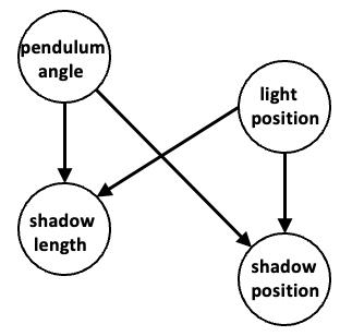
(a) Pendulum

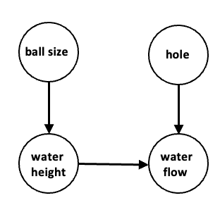
(b) Water Flow

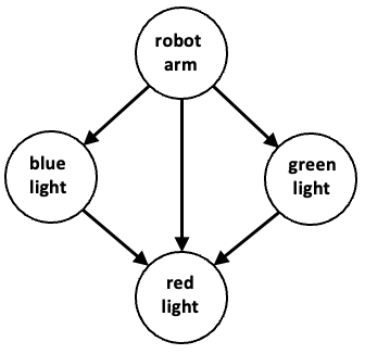
(c) CausalCircuit

Figure 5: Causal Graphs of Datasets

Causal Circuit. The Causal Circuit dataset is a new dataset created by [23] to explore research in causal representation learning. The dataset consists of $512\times 512\times 3$ resolution images generated by $4$ ground-truth latent causal variables: robot arm position, red light intensity, green light intensity, and blue light intensity. The images show a robot arm interacting with a system of buttons and lights. The data is rendered using an open-source physics engine. The original dataset consists of pairs of images before and after an intervention has taken place. For the purposes of this work, we only utilize observational data of either the before or after system. The data is generated according to the following process:

$$v_{R} =0.2+0.6*\text{clip}(u_{2}+u_{3}+b_{R},0,1)$$

$$v_{G} =0.2+0.6*b_{G}$$

$$v_{B} =0.2+0.6*b_{B}$$

$$u_{4} \sim\text{Beta}(5v_{R},5*(1-v_{R}))$$

$$u_{3} \sim\text{Beta}(5v_{G},5*(1-v_{G}))$$

$$u_{2} \sim\text{Beta}(5v_{B},5*(1-v_{B}))$$

$$u_{1} \sim U(0,1)$$

where $b_{R}$, $b_{G}$, and $b_{B}$ are the pressed state of buttons that depends on how far the button is touched from the center, $u_{1}$ is the robot arm position, and $u_{2}$, $u_{3}$, and $u_{4}$ are the intensities of the blue, green, and red lights, respectively. The causal graph is shown in Figure 5(c). From this generative process, we selectively choose only images for which the causal graph is satisfied (the robot arm’s position and the downstream effects). For example, the robot arm appearing over the green button, green button lit up, and red button lit up is consistent with the assumption that the robot arm position causes changes in which buttons light up according to the causal graph. The filtered dataset consists of roughly $35$K training samples and $10$K testing samples.

C.2 Implementation details

For all experiments, we maximize the following ELBO with a bottleneck parameter $\beta$, which controls the degree to which the latent representation is causally factorized.

$$\begin{split}\log p_{\theta}(x,u)\geq\mathbb{E}_{\epsilon,z\sim q_{\phi}(\epsilon,z|x,u)}\Big{[}\log p_{\theta}(x|\epsilon)+\log p_{\theta}(x|z)-\beta\{\log q_{\phi}(\epsilon|x,u)+\log q_{\phi}(z|x,u)\\ -\log p(\epsilon)-\log p_{\theta}(z|u)\}\Big{]}\end{split}$$ (71)

For the Pendulum dataset, we linearly increase the $\beta$ parameter throughout training from $0$ to a final value of $1$ and set a learning rate of $0.001$. We use roughly $6$K samples for training and $1$K samples for testing and train for $8\cdot 10^{3}$ steps using a batch size of $64$. We use a Gaussian encoder and decoder with mean and variance computed by fully connected neural networks.

For the Flow dataset, we linearly increase the $\beta$ parameter throughout training from $0$ to a final value of $1$ and set a learning rate of $0.001$. We use roughly $6$K samples for training and $2$K for testing and train for $8\cdot 10^{3}$ steps using a batch size of $64$. We use a Gaussian encoder and decoder with mean and variance computed by fully connected neural networks.

For the CausalCircuit dataset, we linearly increase $\beta$ from $0$ to a final value of $0.05$ and set a learning rate of $0.001$. We use roughly $35$K samples for training and $10$K samples for testing and train for $3.5\cdot 10^{4}$ steps using a batch size of $100$. We use a convolutional neural network architecture with $6$ layers and ReLU activation followed by a fully connected layer to estimate the mean and variance. The noise level for the variance of the Gaussian distribution of the conditional prior is controlled by $\sigma^{2}\in\{0.01,0.00001\}$.

SCF. The structural causal flow and $\bm{\lambda}$ are implemented as an affine form autoregressive transformation with the slope and offset computed by fully connected three-layer neural networks with $100$ unit hidden layers and ReLU activation. We set the dimension of each causal variable to $4$ for all datasets.

Baselines. We compare ICM-VAE with four baselines: two acausal and two causal.

$\beta$-VAE [24] is an unsupervised disentanglement method that aims to promote disentanglement in the latent space by encouraging the latent representation to be more factorized. However, $\beta$-VAE is unable to effectively disentangle the factors of variation to a high degree, which is consistent with the claim from [2] that unsupervised disentanglement is not possible without additional inductive biases.

iVAE [11] unifies nonlinear ICA and the VAE to develop a framework for learning identifiable representations using auxiliary information in the form of a conditionally factorial prior. However, the framework of iVAE assumes independent factors of variation, which is often an impractical assumption. Due to this assumption, iVAE is unable to disentangle causally related factors.

CausalVAE [13] and SCM-VAE [25] extended the iVAE framework for causally related factors of variation. CausalVAE utilizes a prior that still assumes mutual independence of the factors of variation. Further, CausalVAE assumes a simple linear SCM, which is unrealistic in practice. SCM-VAE builds on this work and consists of a post-nonlinear additive noise SCM and a label-specific causal prior. However, the causal prior proposed still does not induce a causal factorization of latent factors. Thus, CausalVAE and SCM-VAE are also unable to properly disentangle the causal factors.

We note that none of the identifiability results from baselines focus on causal mechanism equivalence. Our proposed prior encourages a causally factorized latent space, which induces a mechanism equivalence and causal disentanglement.

Evaluation Metrics. The DCI metric [20] quantifies the degree to which ground-truth factors and learned latents are in one-to-one correspondence. We compute the DCI disentanglement ($D$) and completeness ($C$) scores, which are based on a feature importance matrix quantifying the degree to which each latent code is important for predicting each ground truth causal factor. The feature importance matrix is computed using gradient-boosted trees (GBT). The informativeness ($I$) score is the prediction error in the latent factors predicting the ground-truth generative factors and is constant ($I=0$) throughout all datasets and models, so we omit it for brevity. We train models with $3$ random seeds and select the median DCI score to report. It is often important that we achieve the robustness of groups of features in the latent variable with respect to interventions on groups of generative factors. To evaluate how changes in the generative factors affect the latent factors, we compute the interventional robustness score (IRS) [22], which is similar to an $R^{2}$ value.

Compute. We run our experiments on an Ubuntu 20.04 workstation with eight NVIDIA Tesla V100-SXM2 GPUs with 32GB RAM.

C.3 Counterfactual Generation

Following [3], the process for obtaining counterfactual predictions consists of three steps

1. Abduction: given an observation $x$, we infer the distribution over the latent variable $\epsilon$ via $\epsilon=a^{-1}(x)$. In the context of ICM-VAE, we have that $z=g^{-1}(x)=f^{RF}(\epsilon)$.

2. Action: substitute the values of $z$ with values based on the counterfactual query $z_{z_{j}\leftarrow\alpha}$

3. Prediction: using the modified model and the value of $z$, compute (decode to) the value of $x$, the consequence of the counterfactual.

Appendix D Related Work

Recently, [2] showed that it is impossible to learn a disentangled representation in an unsupervised manner without some form of inductive bias. Notably, [26] proved that models with an independent prior are not identifiable. Further, [27] showed that most existing disentanglement methods, such as $\beta$-VAE [24], fail to disentangle factors when correlations exist in the data. However, results from large-scale empirical studies [27, 18] have indicated that weak supervision in the form of labels or contrastive data can effectively disentangle correlated or causal factors.

Several modeling paradigms have been recently employed to learn causal representations in the weakly supervised setting by introducing auxiliary information into the data-generating process [8]. Previous work has focused on using supervised labels as auxiliary information to learn disentangled causal representations [11, 13, 25]. Our work builds upon the ideas presented in iVAE [11] and causal variants [13, 25] and extends them to consider a principled view of causal disentanglement in the label supervised setting. [13] proposed a causal masking layer based on [28] and [29] and is limited to linear SCMs. [25] extended this setting to a nonlinear setting and proposed a causal prior. Both works proposed relatively simplistic models to learn causal mechanisms under the strictly additive noise assumption and do not, from an empirical or theoretical perspective, focus on disentanglement. [23] extended [18] to learn causal representations when interventional data is available as pre and post-intervened views, [19] focused on learning causal representations in the temporal setting, and [30] showed identifiability of causal representations in self-supervised learning. Although interesting, studying causal representations in the presence of interventional data can often be an infeasible assumption in practice. Thus, learning robust causal representations from only observational data is desirable. [31] explored the notion of identifiability through independent mechanism analysis. However, they studied an alternative to nonlinear ICA to achieve identifiability. We propose a causal mechanism equivalence definition of identifiability extending upon the iVAE framework to learn mechanism identifiable causal representations.

Appendix E Limitations

We acknowledge that causal discovery is also an important component of causal representation learning. However, developing a causal discovery procedure for general nonlinear causal models, as described in this work, without assuming a simplified form (such as additive noise), is still an open problem [32, 33, 34]. We leave the extension of our work to incorporate causal discovery into the learning process, with and without interventional data, as future work. Another limitation of our current work is that the results only hold for continuous-valued ground-truth variables. We look to extend our framework to be compatible with discrete-valued variables. Further, the DCI metric, although suitable for evaluating disentanglement of causal representations [23], may need to be extended to more robustly incorporate the notion of causal disentanglement. We leave the exploration of such metrics as future work. For this work, we assume labels for all causal variables are observed. Another direction for future work is exploring the extent to which causal disentanglement is still possible when labels are only partially observed.

References

- [1] Yoshua Bengio, Aaron Courville, and Pascal Vincent. Representation learning: A review and new perspectives. IEEE Transactions on Pattern Analysis and Machine Intelligence, 35(8):1798–1828, 2013.
- [2] Francesco Locatello, Stefan Bauer, Mario Lucic, Gunnar Raetsch, Sylvain Gelly, Bernhard Schölkopf, and Olivier Bachem. Challenging common assumptions in the unsupervised learning of disentangled representations. In Proceedings of the 36th International Conference on Machine Learning, 2019.
- [3] Judea Pearl. Causality. Cambridge University Press, Cambridge, UK, 2 edition, 2009.
- [4] Bernhard Scholkopf, Francesco Locatello, Stefan Bauer, Nan Rosemary Ke, Nal Kalchbrenner, Anirudh Goyal, and Yoshua Bengio. Toward Causal Representation Learning. Proceedings of the IEEE, 109(5):612–634, May 2021.
- [5] Giambattista Parascandolo, Niki Kilbertus, Mateo Rojas-Carulla, and Bernhard Schölkopf. Learning independent causal mechanisms. In Proceedings of the 35th International Conference on Machine Learning, 2018.
- [6] Bernhard Schölkopf and Julius von Kügelgen. From statistical to causal learning. arXiv:2204.00607, 2022.
- [7] Jonas Peters, Dominik Janzing, and Bernhard Schlkopf. Elements of Causal Inference: Foundations and Learning Algorithms. The MIT Press, 2017.
- [8] Aapo Hyvarinen, Hiroaki Sasaki, and Richard E. Turner. Nonlinear ica using auxiliary variables and generalized contrastive learning. arXiv:1805.08651, 2018.
- [9] Pierre Comon. Independent component analysis, a new concept? Signal Processing, 36(3):287–314, 1994. Higher Order Statistics.
- [10] Aapo Hyvärinen and Petteri Pajunen. Nonlinear independent component analysis: Existence and uniqueness results. Neural Networks, 12(3):429–439, 1999.
- [11] Ilyes Khemakhem, Diederik Kingma, Ricardo Monti, and Aapo Hyvarinen. Variational autoencoders and nonlinear ica: A unifying framework. In Proceedings of the Twenty Third International Conference on Artificial Intelligence and Statistics, 2020.
- [12] Sebastien Lachapelle, Pau Rodriguez, Yash Sharma, Katie E Everett, Rémi LE PRIOL, Alexandre Lacoste, and Simon Lacoste-Julien. Disentanglement via mechanism sparsity regularization: A new principle for nonlinear ICA. In First Conference on Causal Learning and Reasoning, 2022.
- [13] Mengyue Yang, Furui Liu, Zhitang Chen, Xinwei Shen, Jianye Hao, and Jun Wang. Causalvae: Disentangled representation learning via neural structural causal models. In IEEE Conference on Computer Vision and Pattern Recognition, 2021.
- [14] George Papamakarios, Eric Nalisnick, Danilo Jimenez Rezende, Shakir Mohamed, and Balaji Lakshminarayanan. Normalizing flows for probabilistic modeling and inference. Journal of Machine Learning Research, 22(1), 2021.
- [15] Ilyes Khemakhem, Ricardo Monti, Robert Leech, and Aapo Hyvarinen. Causal autoregressive flows. In Proceedings of The 24th International Conference on Artificial Intelligence and Statistics, 2021.
- [16] Arash Nasr-Esfahany, Mohammad Alizadeh, and Devavrat Shah. Counterfactual identifiability of bijective causal models. In Proceedings of the 40th International Conference on Machine Learning, 2023.
- [17] P. Spirtes, C. Glymour, and R. Scheines. Causation, Prediction, and Search. MIT press, 2nd edition, 2000.
- [18] Francesco Locatello, Ben Poole, Gunnar Rätsch, Bernhard Schölkopf, Olivier Bachem, and Michael Tschannen. Weakly-supervised disentanglement without compromises. In Proceedings of the 37th International Conference on Machine Learning, 2020.
- [19] Phillip Lippe, Sara Magliacane, Sindy Löwe, Yuki M Asano, Taco Cohen, and Efstratios Gavves. Causal representation learning for instantaneous and temporal effects in interactive systems. In The Eleventh International Conference on Learning Representations, 2023.
- [20] Cian Eastwood and Christopher K. I. Williams. A framework for the quantitative evaluation of disentangled representations. In International Conference on Learning Representations, 2018.
- [21] Cian Eastwood, Andrei Liviu Nicolicioiu, Julius Von Kügelgen, Armin Kekić, Frederik Träuble, Andrea Dittadi, and Bernhard Schölkopf. DCI-ES: An extended disentanglement framework with connections to identifiability. In The Eleventh International Conference on Learning Representations, 2023.
- [22] Raphael Suter, Djordje Miladinovic, Bernhard Schölkopf, and Stefan Bauer. Robustly disentangled causal mechanisms: Validating deep representations for interventional robustness. In Proceedings of the 36th International Conference on Machine Learning, 2019.
- [23] Johann Brehmer, Pim De Haan, Phillip Lippe, and Taco Cohen. Weakly supervised causal representation learning. In Advances in Neural Information Processing Systems, 2022.
- [24] Irina Higgins, Loic Matthey, Arka Pal, Christopher Burgess, Xavier Glorot, Matthew Botvinick, Shakir Mohamed, and Alexander Lerchner. beta-VAE: Learning basic visual concepts with a constrained variational framework. In International Conference on Learning Representations, 2017.
- [25] Aneesh Komanduri, Yongkai Wu, Wen Huang, Feng Chen, and Xintao Wu. Scm-vae: Learning identifiable causal representations via structural knowledge. In IEEE International Conference on Big Data (Big Data), 2022.
- [26] Xinwei Shen, Furui Liu, Hanze Dong, Qing Lian, Zhitang Chen, and Tong Zhang. Weakly supervised disentangled generative causal representation learning. Journal of Machine Learning Research, 23(241):1–55, 2022.
- [27] Frederik Träuble, Elliot Creager, Niki Kilbertus, Francesco Locatello, Andrea Dittadi, Anirudh Goyal, Bernhard Schölkopf, and Stefan Bauer. On disentangled representations learned from correlated data. In Proceedings of the 38th International Conference on Machine Learning, 2021.
- [28] Ignavier Ng, Shengyu Zhu, Zhuangyan Fang, Haoyang Li, Zhitang Chen, and Jun Wang. Masked gradient-based causal structure learning. In Proceedings of the 2022 SIAM International Conference on Data Mining (SDM), 2022.
- [29] Xun Zheng, Bryon Aragam, Pradeep K Ravikumar, and Eric P Xing. Dags with no tears: Continuous optimization for structure learning. In Advances in Neural Information Processing Systems, 2018.
- [30] Julius Von Kügelgen, Yash Sharma, Luigi Gresele, Wieland Brendel, Bernhard Schölkopf, Michel Besserve, and Francesco Locatello. Self-supervised learning with data augmentations provably isolates content from style. In Advances in Neural Information Processing Systems, 2021.
- [31] Luigi Gresele, Julius Von Kügelgen, Vincent Stimper, Bernhard Schölkopf, and Michel Besserve. Independent mechanism analysis, a new concept? In Advances in Neural Information Processing Systems, 2021.
- [32] Kun Zhang and Aapo Hyvärinen. Distinguishing causes from effects using nonlinear acyclic causal models. In Proceedings of Workshop on Causality: Objectives and Assessment at NIPS 2008, 2010.
- [33] Ricardo Pio Monti, Kun Zhang, and Aapo Hyvärinen. Causal discovery with general non-linear relationships using non-linear ica. In Proceedings of The 35th Uncertainty in Artificial Intelligence Conference, 2020.
- [34] Patrik Reizinger, Yash Sharma, Matthias Bethge, Bernhard Schölkopf, Ferenc Huszár, and Wieland Brendel. Jacobian-based causal discovery with nonlinear ICA. Transactions on Machine Learning Research, 2023.