Priming bias versus post-treatment bias in experimental designs

Abstract

Conditioning on variables affected by treatment can induce post-treatment bias when estimating causal effects. Although this suggests that researchers should measure potential moderators before administering the treatment in an experiment, doing so may also bias causal effect estimation if the covariate measurement primes respondents to react differently to the treatment. This paper formally analyzes this trade-off between post-treatment and priming biases in three experimental designs that vary when moderators are measured: pre-treatment, post-treatment, or a randomized choice between the two. We derive nonparametric bounds for interactions between the treatment and the moderator in each design and show how to use substantive assumptions to narrow these bounds. These bounds allow researchers to assess the sensitivity of their empirical findings to either source of bias. We then apply these methods to a survey experiment on electoral messaging.

Keywords: bounds, interactions, heterogeneous effects, measurement, moderation, sensitivity analysis

1 Introduction

Ascertaining heterogeneous treatment effects is an integral part of many survey experiments. Researchers are often interested in how treatment effects vary across respondents with different characteristics. For example, we may be interested both in how implicit versus explicit racial cues affect support for a particular policy but also in how those effects differ by levels of racial resentment (Valentino, Hutchings and White, 2002). Or we may want to know whether the effect of land-based electoral appeals might depend on the voters’ sense of land security (Horowitz and Klaus, 2020). These questions of effect heterogeneity allow researchers to explore potential causal mechanisms and design more targeted and effective future treatments.

To examine such treatment effect heterogeneity, we must measure the relevant covariates, such as racial resentment or land security, at some point during the survey experiment. The question of when we measure these covariates, however, is a source of methodological debate. On the one hand, a long tradition in political science has recognized the potential priming bias of a pre-test design, where covariates are measured prior to treatment (e.g., Transue, 2007; Morris, Carranza and Fox, 2008; Klar, 2013; Klar, Leeper and Robison, Forthcoming; Schiff, Montagnes and Peskowitz, 2022). For example, asking a respondent about their party identification might lead them to evaluate the treatment in a more partisan or political light, resulting in a biased causal effect estimate. Several studies have documented priming effects from a range of different covariates (see Klar, Leeper and Robison, Forthcoming, for a review), and certain priming effects can last for weeks (Chong and Druckman, 2010).

On the other hand, the practice of measuring covariates after treatment, what we call a post-test design, has come under scrutiny due to the possibility for post-treatment bias (Rosenbaum, 1984; Acharya, Blackwell and Sen, 2016; Montgomery, Nyhan and Torres, 2018). In particular, if covariates are affected by the treatment, then conditioning on those covariates—as is typical when assessing effect heterogeneity—can bias the estimation of conditional average treatment effect and thus any interactions that compare such effects. In our empirical application, the key moderating variable of land insecurity is a subjective, perceived measure and thus potentially affected by the framing of a political appeal around land rights. Though treatment is unlikely to affect measurements of many moderators like basic demographics, researchers investigating manipulable moderators face a dilemma about when to measure these covariates when designing an experiment.

In this paper, we formally analyze the trade-off between priming and post-treatment biases under different experimental designs, and propose principled ways to analyze data (see Imai and Yamamoto, 2010, for a similar analysis of measurement error). We begin by deriving nonparametric bounds to show that neither the pre-test nor post-test design provides much information about conditional average treatment effects without additional assumptions. Next, we show how two potentially plausible assumptions can narrow the bounds under the post-test design. The first is the monotonicity of the post-test effect, which assumes that measuring the covariates after treatment can move those covariates only in one direction. The second assumption is stable moderator under control, whereby the covariate under the control condition cannot be affected by the timing of treatment. Neither of these assumptions can point identify the interaction between the treatment and a moderator, but they can significantly narrow the bounds and sometimes be informative about the sign of such an interaction.

We also derive a sensitivity analysis procedure, where we vary the maximum magnitude of the discrepancy between the pre- and post-test moderator of interest that can exist and assess how the bounds change as a function of this sensitivity parameter. The proposed sensitivity analysis provides both the researcher and readers with the ability to gauge the credibility of a post-test result in light of their own assumptions.

To further sharpen our inference, we generalize the two standard experimental designs and consider a randomized placement design, where the experimenter randomly assigns respondents to either the pre-test or post-test design. We apply our nonparametric bounding approach and sensitivity analysis to this alternative design to examine how combining information from the pre-test and post-test arms might improve our ability to identify heterogeneous causal effects from a survey experiment. In our supplemental materials, we also develop a parametric Bayesian approach to incorporate pre-treatment covariates in the analysis to sharpen our inferences and quantify estimation uncertainty.

Several recent studies have empirically explored the trade-off between priming and post-treatment bias in particular experimental settings. Albertson and Jessee (2022) find that the effect of moderator placement has little effect on the estimated interaction in a question-wording experiment. Furthermore, they find no evidence for an average effect of treatment on the moderator, potentially reducing concerns about post-treatment bias. Sheagley and Clifford (2023) compared several experiments when the moderators were measured just prior to treatment or in a prior survey wave. The authors found that estimated effects and interactions were similar across these conditions and concluded that priming bias may not be a widespread concern for experimental studies in political science.

Both of these papers present compelling evidence for the specific experiments conducted in their empirical assessments, but it is difficult to generalize these results to other experiments. Our approach, on the other hand, provides a general methodological toolkit that can apply to any experimental design and allows researchers to include substantive assumptions to tailor the framework to their applications.

The rest of the paper proceeds as follows. We first introduce a motivating empirical example of how land insecurity moderates the effectiveness of land-based appeals by politicians from Horowitz and Klaus (2020). We next describe the notation and basic assumptions of the pre-test and post-test designs. We then derive the sharp nonparametric bounds and sensitivity analyses for the pre-test, post-test, and randomized placement designs. Next, we apply the proposed methods to the empirical example. Finally, we conclude by suggesting directions for future research.

2 Motivating Example

We illustrate the trade-off between the pre- and post-treatment measurement of a moderator using a survey experiment conducted by Horowitz and Klaus (2020). In this study, the authors investigated whether politicians can use land-based grievances to increase their electoral support in Kenya’s Rift Valley. Participants were randomly assigned to one of three treatment conditions. In the “control” condition, participants heard a generic campaign speech with no direct reference to the land issue. In the first treatment condition (T1), the candidate additionally states that the land issue is their top priority. In the second treatment condition (T2), the researchers added another sentence to the speech in which the candidate references an ethnic grievance, blaming “migrants and land grabbers.” To preserve statistical power, we collapse the distinction between the conditions T1 and T2 and focus on the effect of a speech referencing the land issue (either T1 or T2) versus not (the “control” speech). The outcome is the participant’s reported likelihood of supporting the candidate, which we dichotomize (likely to support the candidate vs. not) to illustrate our proposed methods.

One of the main hypotheses tested by Horowitz and Klaus (2020) is whether individuals who are personally experiencing land insecurity are more responsive to land-based appeals by politicians. While the evidence from the full sample is inconclusive, among respondents belonging to the “insider” ethnic group (Kalenjins), there is a positive and statistically significant interaction between the treatment conditions (T1 and T2) and a dummy variable for land insecurity, in line with the authors’ expectations (with the outcome on a 5-point numeric scale, $\hat{\beta}_{T1:LI}=1.77$, $p=0.01$; $\hat{\beta}_{T2:LI}=1.71$, $p=0.005$).

Both priming bias and post-treatment bias could be a concern in this context, as land insecurity is measured by asking respondents to rate the security of their land rights. Asking this question before treatment may raise the salience of the land issue and thus attenuate any treatment effect of hearing a land-based appeal by a politician, which is a form of priming bias. Conversely, if the experimenter asks respondents about land security after treatment, then their responses may be affected by the content of the speech, yielding a post-treatment bias.

To address these concerns, Horowitz and Klaus (2020) use (what we call) the randomized placement design, in which questions relating to the respondent’s land rights were randomly assigned to occur before or after the treatment. With this design, researchers can compare estimates of the quantity of interest produced using the pre-test or post-test data only, as well as the combined sample. As shown in Figure 1, the “naïve” estimates of the treatment-moderator interaction obtained from a linear probability model on different subsets of the data are qualitatively similar. All the point estimates are positive and substantively large, implying that the effect of a land-based appeal on electoral support is 25–50 percentage points larger for respondents who are land insecure compared to those who are not. However, these estimates only reach conventional levels of statistical significance with the increased statistical power of the combined pre/post sample. The point estimates from the post-test data are particularly sensitive to the inclusion of covariates.

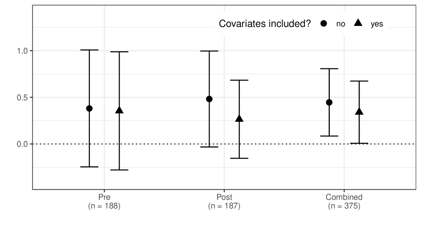
Figure 1: Estimates of treatment-moderator interaction using pre-test, post-test, and combined data.

Notes: Figure shows point estimates and 95% confidence intervals for the interaction between treatment and land insecurity on candidate support from a linear probability model, using the pre-test data (moderator measured before treatment), the post-test data (moderator measured after treatment), and the combined sample from Horowitz and Klaus (2020). Estimates are shown from models with and without covariates. We follow the original authors in using age, gender, education, and closeness to own ethnic group as covariates.

Empirical investigations into post-treatment and priming biases for this study reveal mixed results. To investigate possible post-treatment bias, we can subset the data to the post-test sample and estimate the average treatment effect on the reported land insecurity. Compared to the control condition, respondents who saw the land-based appeal tended to report higher levels of perceived land security, using the original 3-point scale ($\hat{\beta}=0.18$, $p=0.03$). This raises the possibility of post-treatment bias.

The original authors also examine whether estimates of the overall ATE from the pre-test data suffered from priming bias by interacting the treatment variables with a dummy variable for the random placement of the covariate measurement. Although they find null results (Horowitz and Klaus, 2020, Table A14), this analysis does not directly speak to the question of whether priming bias is present in estimates of the effect heterogeneity themselves. In fact, even under the randomized placement design, the observed data cannot provide a complete answer to this question since the treatment-moderator interaction is not identified (see Sections 4.1 and 4.2). In Section 5, we return to this empirical example to illustrate how researchers can assess the possible impact of priming bias and post-treatment bias on their substantive findings using our proposed methods.

3 Experimental Designs and Causal Quantities of Interest

We now lay out the formal notation of our setting and describe the causal quantities of interest. Suppose we have a simple random sample of size $n$ from a population of interest. Let $T_{i}$ represent the binary treatment variable for unit $i$, indicating a certain experimental manipulation received by the unit. We use $Y_{i}$ to denote an outcome of interest, and $M_{i}$ to represent an observed binary covariate and moderator of interest. Our goal is to develop a methodology that can be used to understand how the effect of $T_{i}$ on $Y_{i}$ varies as a function of $M_{i}$.

In this paper, we consider three experimental designs for this goal: the pre-test design, the post-test design, and the randomized placement design. These three designs differ in the timing of measurement for the potential moderators. In the pre-test design, the experimenter measures the moderator, $M_{i}$, before treatment assignment, ensuring that these measurements are unaffected by treatment. In the post-test design, the experimenter measures moderators after treatment assignment. We let $Z_{i}$ be an indicator for whether the experiment measures $M_{i}$ before ($Z_{i}=0$) or after treatment ($Z_{i}=1$). The randomized placement design randomly assigns $Z_{i}$ along with treatment, so only a random subset of units can have treatment affect their moderator.

We will analyze these experimental designs using the potential outcomes framework for causal inference (e.g., Holland, 1986). Let $Y_{i}(t,z)$ represent the potential outcome with respect to the treatment status $t$ and the timing of covariate measurement, $z$. We assume that the potential outcomes are binary variables fixed for each unit $i$, i.e., $Y_{i}(t,z)\in\{0,1\}$ for all $(t,z)\in\{0,1\}^{2}$, though many of the methods below could be modified to handle multi-valued outcomes. We make the consistency assumption for the potential outcomes, such that $Y_{i}=Y_{i}(T_{i},Z_{i})$.

Suppose that researchers wish to estimate treatment effects on the outcome free of priming bias, or when moderators are measured after treatment. We define these “true” potential outcomes of interest as $Y^{*}_{i}(t)\equiv Y_{i}(t,1)$ and let $Y_{i}(t)\equiv Y_{i}(t,0)$ to be a possibly mismeasured proxy we observe in the pretest design. In general, however, the potential outcomes for the pre- and post-test designs will differ so that $Y_{i}(t)\neq Y^{*}_{i}(t)$. This difference corresponds to priming bias.

Similarly, the measures of the moderator can be affected by the experimental design and the administered treatment. Let $M_{i}(t,z)$ be the potential value of the moderator that would be observed for unit $i$ when the treatment is set to $t$ and the variable is measured in design $z$. We assume this moderator is binary so that $M_{i}(t,z)\in\{0,1\}$, and make the consistency assumption such that $M_{i}=M_{i}(T_{i},Z_{i})$. Under the pre-test design, the treatment cannot affect the moderator, so we refer to $M_{i}(0,0)=M_{i}(1,0)\equiv M^{*}_{i}$ as the “true” moderator for unit $i$ at the time of the experiment. On the other hand, under the post-test design, we let $M_{i}(t)\equiv M_{i}(t,1)$ to be potentially mismeasured proxy for that true moderator. In those designs, the treatment can affect respondents’ moderator (turning it into a mediator), so that $M_{i}(0)\neq M_{i}(1)$, which can lead to post-treatment bias.

Given the above notation, the causal moderation effects can be explored by estimating the following quantities of interest,

$$\tau(m) \equiv \mathbb{E}(Y_{i}^{*}(1)-Y^{*}_{i}(0)\mid M^{*}_{i}=m),$$ (1)

$$\delta \equiv \tau(1)-\tau(0),$$ (2)

where $m\in\{0,1\}$. The first quantity, $\tau(m)$, characterizes the post-test conditional average treatment effect (CATE) as a function of the pre-test effect modifier. The second quantity of interest, $\delta$, compares the CATE between two subpopulations with different levels of the pre-test moderator, which we sometimes refer to as the interaction.

These two quantities of interest formalize the dilemma about the choice of pre-test versus post-test experimental designs. There are four different possible worlds defined by the treatment and the pre- versus post-test experimental design, and we only observe outcomes for one of these worlds. The problem is that the true potential outcomes of interest ($Y^{*}_{i}(t)$) and true moderator ($M^{*}_{i}$) can never be jointly observed for the same unit.

While the pre-test design allows us to observe the true moderator, it may suffer from priming bias because asking questions about the moderator might change the causal effect of the treatment by cueing respondents. Thus, under the pre-test design, neither $\tau(m)$ nor $\delta$ is identified. Indeed, even the overall ATE cannot be identified for the “true” outcome of interest despite the randomization of the treatment. This overall ATE can be written as,

$$\tau \equiv \mathbb{E}(Y^{*}_{i}(1)-Y^{*}_{i}(0)).$$ (3)

In contrast, under the post-test design, the overall ATE can be estimated without bias, and yet this design may result in post-test bias for $\tau(m)$ and $\delta$ when the treatment affects the moderator. In sum, the dilemma is that we are interested in how the effects on the post-test outcome vary by pre-test moderator levels, but we cannot simultaneously assign the same individual to both designs.

4 Nonparametric Analysis of the Three Experimental Designs

We first analyze the pre- vs. post-test designs without parametric assumptions. We begin by showing that, without further assumptions, neither the pre-test nor post-test design is informative of the CATEs or the differences between CATEs. We then derive sharp bounds for the interaction between the treatment and the moderator under the post-test design and show how to narrow these bounds with additional assumptions. We also develop a sensitivity analysis procedure, which allows researchers to vary the strengths of such assumptions and assess their implications. Finally, we examine the random placement design using similar analytical approaches.

4.1 Uninformativeness of the Pre-test Design

We first consider the identifying power of the pre-test design, where we observe $(Y_{i},M_{i},T_{i})$ among the units for whom $Z_{i}=0$. Under this design, the randomization of the treatment guarantees the following statistical independence between potential outcomes and the treatment variable.

Assumption 1 (Pre-test Randomization).

$$\{Y_{i}(t,z),M_{i}(t,1)\}\ \mbox{$\perp\!\!\!\perp$}\ T_{i} \mid M^{*}_{i}=m,Z_{i}=0,$$ (4)

for $t=0,1$, $m\in\{0,1\}$ and all $i$.

This assumption allows for the possibility of conditioning our randomization on the pre-treatment moderator, though this assumption also holds when randomization is unconditional.

By computing the difference in average observed outcomes between different treatment groups, researchers can identify the following quantity,

$$\tau_{pre}(m) \equiv \mathbb{E}(Y_{i}\mid T_{i}=1,M_{i}=m,Z_{i}=0)-\mathbb{E}(Y_{i}\mid T_{i}=0,M_{i}=m,Z_{i}=0)$$ (5)

$$= \mathbb{E}(Y_{i}(1)-Y_{i}(0)\mid M^{*}_{i}=m),$$

where the equality follows from Assumption 1 and the consistency assumption. Equation (5) does not generally equal the true CATE, $\tau(m)$, since the conditional distribution of $Y_{i}(t)$ given $M^{*}_{i}=m$ may differ from that of $Y^{*}_{i}(t)$ given $M^{*}_{i}=m$, since asking questions about the moderator before measuring outcome may distort subsequent responses. Similarly, $\delta$ is not generally equal to $\delta_{pre}\equiv\tau_{pre}(1)-\tau_{pre}(0)$. The key problem here is that the pre-test design gives us information about the correct values of the moderator $M^{*}_{i}$, but provides no information about the outcomes we want to investigate, $Y^{*}_{i}(t)$.

Without any assumptions on how severe such priming bias could be, we cannot rule out extreme possibilities, such as all respondents changing their values of $Y_{i}$ in response to the priming (that is, all $Y_{i}=1$ switching to $Y_{i}=0$ and vice versa). Thus, even under randomization, the no-assumption bounds under the pre-test design remain identical to the original bounds,

$$\tau(m) \in [-1,\ 1],$$ (6)

$$\delta \in [-2,\ 2].$$ (7)

In other words, the pre-test design is completely uninformative about the causal effects of interest unless one is willing to make additional assumptions about the joint distribution of $Y^{*}_{i}(t)$ and $Y_{i}(t)$. Of course, such assumptions are not testable under the pre-test design. This implies that, in theory, the priming bias can be arbitrarily large, and that the observed data do not contain any direct information about the magnitude of such bias.

4.2 Limited Informativeness of the Post-test Design

Next, we consider the post-test design, where we observe $(Y_{i},M_{i},T_{i})$ among the units for whom $Z_{i}=1$. The randomization of the treatment implies the following ignorability assumption.

Assumption 2 (Post-Test Randomization).

$$\{Y_{i}(t,z),M_{i}(t),M^{*}_{i}\}\ \mbox{$\perp\!\!\!\perp$}\ T_{i}\mid Z_{i}=1,$$

for $t=0,1$.

How informative is Assumption 2 alone about the CATEs and interaction without making any other assumption? Let $P_{tzm}=\mathbb{P}(Y_{i}=1\mid T_{i}=t,Z_{i}=z,M_{i}=m)$ and $Q_{tz}=\Pr(M_{i}=1\mid T_{i}=t,Z_{i}=z)$ be the conditional outcome and moderator distributions. Then, the standard CATE estimator would be unbiased for $\tau_{post}(m)\equiv P_{11m}-P_{01m}$. Under the post-test design, we can connect this quantity to the following counterfactual contrast,

$$\tau_{post}(m) \equiv P_{11m}-P_{01m}=\mathbb{E}[Y^{*}_{i}(1)\mid M_{i}(1)=m]-\mathbb{E}[Y^{*}_{i}(0)\mid M_{i}(0)=m],$$ (8)

where the equality follows from Assumption 2 and the fact that $\Pr(Z_{i}=1)=1$ for all $i$.

Under the post-test design, we observe the true potential outcome of interest $Y_{i}^{\ast}(t)$, and yet the moderator may be observed with error, i.e., $M_{i}(t)\neq M_{i}^{\ast}$. Similar to the case of the pre-test design, therefore, $\tau_{post}(m)$ does not generally equal $\tau(m)$ because the conditional distribution of $Y^{*}_{i}(t)$ given $M_{i}(t)=m$ may differ from that of $Y^{*}_{i}(t)$ given $M^{*}_{i}=m$. In fact, $\tau_{post}(m)$ is not necessarily the same as $\tau(m)$ even if the effects of treatment and moderator measurement timing do not change the marginal distribution of the moderator, i.e., $\Pr(M_{i}(0)=m)=\Pr(M_{i}(1)=m)=\mathbb{P}(M_{i}^{*}=m)$ for all $m\in\mathcal{M}$. Restricting the marginal distribution of the moderator does not help because effect heterogeneity is a function of the joint distribution of the counterfactual outcomes and moderators. Thus, under the post-test design, neither $\tau(m)$ nor $\delta$ is nonparametrically identified.

Even though the post-test design does not point-identify the CATEs or the interaction, the design can contain some information about the causal quantities of interest. The following proposition derives the sharp (i.e., shortest possible) no-assumption bounds under the post-test design.

Proposition 1 (No-assumption Post-test Bounds).

Let $P_{t}=\mathbb{P}(Y_{i}=1\mid T_{i}=t,Z_{i}=1)$. Under Assumptions 2, we have $\delta\in[\delta_{L},\delta_{U}]$, where

$$\delta_{L} =-1-\max\left\{\min\left(\frac{1-P_{0}}{P_{1}},\frac{1-P_{1}}{P_{0}}\right),\min\left(\frac{P_{1}}{1-P_{0}},\frac{P_{0}}{1-P_{1}}\right)\right\},$$ (9)

$$\delta_{U} =1+\min\left\{\max\left(\frac{1-P_{0}}{P_{1}},\frac{1-P_{1}}{P_{0}}\right),\max\left(\frac{P_{1}}{1-P_{0}},\frac{P_{0}}{1-P_{1}}\right)\right\}.$$

Furthermore, these bounds are sharp.

The proofs of this result is given in Section A.1 and rely on a standard linear programming approaches often used in bounding causal quantities (e.g., Balke and Pearl, 1997). Unfortunately, these bounds are often quite wide in practice. In particular, it is clear that the bounds can never be narrower than $[-1,1]$. A primary reason for this width is that the observed data under the post-test design are completely uninformative about the true moderator. As a result, the sharp bounds under the post-test design can be quite wide and sometimes cover the entire possible range, $[-2,2]$, for $\delta$. In sum, without additional assumptions, the post-test design can only provide limited information about the causal quantities of interest.

4.3 Narrowing the Post-test Bounds under Additional Assumptions

While the bounds only using the randomization can be too wide to be useful in practice, we may be willing to entertain other assumptions on the causal structure that will allow us to narrow the bounds. We focus here on the post-test design since it has the benefit of ensuring identification of the ATE, but similar analysis can be conducted for the pre-test design (e.g., consider Assumption 5 below).

To narrow our bounds, we rely on a principal stratification approach in which we stratify the units in the study according to their potential responses to treatment on various outcomes (Frangakis and Rubin, 2002). In particular, we create strata based on how the moderator responds to both the treatment and pre-post indicators. Let $\mu_{s}(t)=\mathbb{P}[Y^{*}_{i}(t)=1\mid S_{i}=s]$, where $S_{i}$ represents the principal strata defined by the moderator, $\{M_{i}(1),M_{i}(0),M^{*}_{i}\}$. Without making any assumption, $S_{i}$ can take any of the $2^{3}$ values in

$$\mathcal{S}=\{111,011,101,001,110,010,100,000\}.$$

Let $\rho_{s}=\Pr[S_{i}=s]$ be the probability of a unit falling into one of the strata, such that $\sum_{s\in\mathcal{S}}\rho_{s}=1$. Finally, we denote the marginal probability of the true pre-test moderator as $Q_{*}=\mathbb{P}(M^{*}_{i}=1)$.

4.3.1 Monotonicity and Stable Moderator Assumptions

The first assumption we consider is that the effect of post-treatment measurement of the moderator has a monotonic effect on the moderator for every unit.

Assumption 3 (Monotonicity of the Post-Test Effect).

$M_{i}(t)\geq M^{*}_{i}$ or $M_{i}(t)\leq M^{*}_{i}$ for all $t=0,1$.

In the context of the motivating example, this assumption would require hearing a land-based appeal by a politician to shift perceived land insecurity in the same direction for all respondents (or have no effect). Obviously, the plausibility of this assumption will depend on the experimental context. In most of the paper, we focus on the positive version of this monotonicity assumption. This assumption rules out several possible principal strata, ensuring that $S_{i}$ can only take one of the following values: $111,110,010,100,$ or $000$. While we present the monotonicity assumption in a particular direction for both treatment levels, it is possible to derive bounds under a monotonicity assumption with differing directions for each treatment condition.

Proposition 2 (Post-test Bounds under Monotonicity).

Under Assumptions 2 and 3, we have sharp bounds $\delta\in[\delta_{L2},\delta_{U2}]$, where

$$\delta_{L2} =\frac{P_{111}Q_{11}-P_{011}Q_{01}}{Q_{*}}-\frac{P_{110}(1-Q_{11})-P_{010}(1-Q_{01})}{1-Q_{*}}$$

$$\qquad+\frac{\max\{P_{011}Q_{01}-Q_{*},0\}-\min\{P_{111}Q_{11},Q_{11}-Q_{*}\}}{Q_{*}(1-Q_{*})},$$

$$\delta_{U2} =\frac{P_{111}Q_{11}-P_{011}Q_{01}}{Q_{*}}-\frac{P_{110}(1-Q_{11})-P_{010}(1-Q_{01})}{1-Q_{*}}$$

$$\qquad+\frac{\min\left\{0,Q_{*}-P_{111}Q_{11}\right\}+\min\left\{P_{011}Q_{01},Q_{01}-Q_{*}\right\}}{Q_{*}(1-Q_{*})}.$$

We provide the derivation of these bounds (and those in the next proposition) in Section A.2. Inspection of these functions reveals that we can find the maximum of the upper bound by comparing when $Q_{*}$ makes one of the two minimum statements into equalities, $Q_{*}=P_{111}Q_{11}$ or $Q_{*}=(1-P_{011})Q_{01}$.

These bounds will differ from the above randomization bounds given in Proposition 1 in two ways. First, with the randomization assumption alone, we could only leverage the observed strata within levels of treatment—further stratification in terms of the moderator provided no information because it places no restriction on the relationship between the pre-test and post-test versions of the moderator. Under monotonicity (Assumption 3), we can leverage $P_{tzd}$ and $Q_{tz}$ to narrow the bounds. Second, monotonicity places bounds on the true value of $Q_{*}$ since it must be less than $\min(Q_{11},Q_{01})$.

While the post-test monotonicity assumption does narrow the bounds, they are often still quite wide and usually contain 0. To further narrow the bounds, we consider another assumption that the moderator is stable in the control arm of the study.

Assumption 4 (Stable Moderator under Control).

$M^{*}_{i}=M_{i}(0)$

This assumption implies that the moderator under control in the post-test design is the same as the moderator as if it was measured pre-test. This assumption may be plausible in experimental designs where the control condition is neutral or similar to the pre-test environment. In our empirical example, this would mean that hearing the generic campaign speech, which does not mention the land issue, does not affect perceived land insecurity. Under both Assumptions 3 and 4, the only values that principal strata that $S_{i}$ can take are $\{111,100,000\}$.

Proposition 3 (Post-test Bounds under Monotonicity and Stability).

Under Assumptions 2, 3, and 4, we have $Q_{*}=Q_{01}$ and sharp bounds $\delta\in[\delta_{L3},\delta_{U3}]$, where

$$\delta_{L3} =\frac{P_{111}Q_{11}}{Q_{01}}-P_{011}-\frac{P_{110}(1-Q_{11})}{1-Q_{01}}+P_{010}-\min\left\{1,\frac{P_{111}Q_{11}}{Q_{11}-Q_{01}}\right\}\cdot\frac{Q_{11}-Q_{01}}{Q_{01}(1-Q_{01})},$$

$$\delta_{U3} =\frac{P_{111}Q_{11}}{Q_{01}}-P_{011}-\frac{P_{110}(1-Q_{11})}{1-Q_{01}}+P_{010}-\max\left\{0,\frac{P_{111}Q_{11}-Q_{01}}{Q_{11}-Q_{01}}\right\}\cdot\frac{Q_{11}-Q_{01}}{Q_{01}(1-Q_{01})}.$$

These bounds demonstrate how the magnitude of treatment effect on the moderator affects identification in the post-test design. A unit’s moderator is affected by treatment whenever $M_{i}(1)\neq M_{i}(0)$, which corresponds to the $S_{i}=100$ principal stratum under monotonicity and stable moderator under control. Note that under these assumptions, $\rho_{100}$ represents the magnitude of the treatment-moderator effect. Since $Q_{11}=\rho_{111}+\rho_{100}$ and $Q_{01}=\rho_{111}$, we can identify this effect with the usual difference in (population) means, $Q_{11}-Q_{01}=\rho_{100}$. The maximum possible width of the sharp bounds depends on this effect, with

$$\max\{\delta_{U3}-\delta_{L3}\}=\frac{Q_{11}-Q_{01}}{Q_{01}(1-Q_{01})}=\frac{\rho_{100}}{\rho_{000}(\rho_{111}+\rho_{100})},$$

so that the bounds can be relatively informative if the post-treatment average effect on the moderator is small.

4.3.2 Sensitivity Analysis under Limited Effects on the Moderator

While the monotonicity and stable moderator assumptions can considerably narrow the nonparametric bounds on our causal quantities, they rule out entire principal strata, which may be stronger than is justified for a particular empirical setting. To address this limitation, we now consider an alternative approach to bounds that does not rule out any particular principal strata, but rather places restrictions on the proportion of units whose moderators are affected by treatment.

In particular, we propose a sensitivity analysis that limits the proportion of respondents whose moderator value changes between the pre-test and post-test values, regardless of the treatment condition (contrast this with Assumption 4 which applies to the control condition only). We operationalize this via the following constraint,

$$\Pr(S_{i}\notin\{111,000\})\leq\gamma.$$

Note that $\gamma$ must be greater than $|Q_{11}-Q_{01}|$ for the bounds to be feasible since $|Q_{11}-Q_{01}|=|\rho_{101}+\rho_{100}-\rho_{011}-\rho_{010}|$. We vary the value of $\gamma$ from $|Q_{11}-Q_{01}|$ to $1$ and see how the nonparametric bounds on the value of $\delta$ change as we gradually allow a larger treatment effect on the moderator. We obtain these new bounds by adding this additional constraint to the second step of the above constrained optimization procedure. This approach is a more flexible way to allow for limited heterogeneous treatment effects on the moderator in any direction. Researchers can also combine this sensitivity analysis with the monotonicity and stable moderator assumptions.

4.3.3 Statistical Inference

The above bounding procedures assume that we observe the conditional probabilities $P_{tzd}$ perfectly when, in fact, we only have estimates of these quantities. Thus, the bounds derived above do not account for estimation uncertainty. To resolve this, we rely on the approach of Imbens and Manski (2004) to derive confidence intervals for the underlying parameters of interest that take into account their partial identification. These confidence intervals are designed to provide nominal coverage for the (partially identified) causal quantity of interest rather than nominal coverage for the true bounds. This procedure requires estimates of the variance of bounds, which we obtain via the nonparametric bootstrap similarly to Horowitz and Manski (2000).

In the supplemental materials, we also develop a model-based approach to incorporate additional pre-treatment covariates that might be available to researchers. One limitation of nonparametric bounds and sensitivity analyses is the difficulty of incorporating a large number of covariates, which may provide additional information and sharpen our inference. Our parametric Bayesian approach accommodates such covariates in a flexible manner and produces estimates of statistical uncertainty (Mealli and Pacini, 2013). Our proposed algorithm takes advantage of a recent advance in Bayesian analysis for binary and multinomial logistic regression models, which allows for fast, computationally efficient estimation of our causal quantities of interest (Polson, Scott and Windle, 2013).

4.4 Analysis of the Randomized Placement Design

Finally, we consider a combined pre/post design called the randomized placement design, where in addition to treatment, the timing of covariate measurement, $Z_{i}$, is also randomized. Under the randomized placement design, the bounds from the post-test alone can be tightened because we can identify the marginal probability of the true moderator as

$$Q_{*}\ =\ \Pr(M^{*}_{i}=1)\ =\ \Pr(M_{i}=1\mid Z_{i}=0).$$

Unfortunately, for the randomization bounds in Equation (9), the sign of $\delta$ cannot be identified for any value of $Q_{*}\in(0,1)$. However, under the assumption of monotonicity for the moderator (Assumption 3), the bounds can be informative.

With the randomized placement design, we have a slightly more complicated set of principal strata since now we must handle both the pre-test and post-test potential outcomes. In particular, we have the following:

$$\psi_{y_{1}y_{0}s}(t)\ =\ \Pr(Y^{*}_{i}(t)=y_{1},Y_{i}(t)=y_{0}\mid S_{i}=s)$$

where $\psi_{y_{1}y_{0}s}(t)\geq 0$ and $\sum_{y_{1}}\sum_{y_{0}}\psi_{y_{1}y_{0}s}(t)=1$ for all $t$. These values characterize the joint distribution of the pre-test and post-test potential outcomes for a given treatment level, $t$, and principal strata, $s$. Furthermore, let $\mathcal{S}^{*}_{m}=\{s:s\in\mathcal{S},M^{*}_{i}=m\}$ be the set of principal strata with the true value of the moderator equal to $d$.

Given these, we can write the interaction between the treatment and the moderator as

$$\delta\ =\ \sum_{y_{0}=0}^{1}\left\{\sum_{s_{1}\in\mathcal{S}^{*}_{1}}\frac{\rho_{s_{1}}}{Q_{*}}(\psi_{1y_{0}s_{1}}(1)-\psi_{1y_{0}s_{1}}(0))-\sum_{s_{0}\in\mathcal{S}^{*}_{0}}\frac{\rho_{s_{0}}}{1-Q_{*}}(\psi_{1y_{0}s_{0}}(1)-\psi_{1y_{0}s_{0}}(0))\right\},$$

and the observed strata in the pre-test and post-test arms as

$$P_{t1m}Q_{t1} =\Pr(Y_{i}=1,D_{i}=m\mid T_{i}=t,Z_{i}=1)\ =\ \sum_{y_{0}=0}^{1}\sum_{s\in\mathcal{S}(t,1,m)}\psi_{1y_{0}s}(t)\rho_{s},$$

$$P_{t0m_{\ast}} =\Pr(Y_{i}=1\mid T_{i}=t,Z_{i}=0,M_{i}=m_{\ast})=\frac{\sum_{y_{1}=0}^{1}\sum_{s\in\mathcal{S}^{*}_{m_{\ast}}}\psi_{y_{1}1s}(t)\rho_{s}}{\sum_{s\in\mathcal{S}^{*}_{m_{\ast}}}\rho_{s}},$$

for all values of $y$, $m$, $t$, and $m_{\ast}$.

4.4.1 Bounds under Priming Monotonicity

Without further assumptions, the pre-test data are helpful only insofar as they identify the marginal distribution of the moderator, $Q_{*}$. However, additional assumptions about the connection between the pre- and post-test data can be informative. We consider a priming monotonicity assumption, which states that the effect of asking the moderator before treatment can only move the outcome in a single direction.

Assumption 5 (Priming Monotonicity).

$Y_{i}(t)\geq Y^{*}_{i}(t)$ for all $t=0,1$.

The assumption implies that the effect of moving from post-test ($Z_{i}=1$) to pre-test ($Z_{i}=0$), which we call the priming effect, can only increase the outcome. In the context of our application, this assumption implies that asking about land rights before reading the campaign speech treatment increases support for the hypothetical candidate. As stated, this assumption holds across levels of treatment, though it is possible to assume the reverse direction ($Y_{i}(t)\leq Y^{*}_{i}(t)$) or even to have a different effect direction for each level of treatment.

As with moderator monotonicity, priming monotonicity implies restrictions on the principal strata that help narrow the bounds on the CATEs and interactions. In particular, priming monotonicity implies that $\psi_{10s}=0$ for any value of $s\in\mathcal{S}$. To obtain bounds under this assumption, we again can numerically solve the above linear programming problem subject to these restrictions. Furthermore, it is possible to combine this priming monotonicity with moderator monotonicity and narrow the bounds even further.

4.4.2 Sensitivity Analysis

With this setup, we can also develop a sensitivity analysis procedure based on substantive assumptions about how much the pre-test vs. post-test measurement of the moderator affects the moderator itself and the outcome. The first of these is the sensitivity analysis described above for the post-test design now adapted to the principal strata of the randomized placement design:

$$\Pr(S_{i}\notin\{111,000\})\leq\ \gamma.$$

Again, this assumption constrains the proportion of the respondents whose moderator value is affected by $Z_{i}$ in either treatment arm. If $\gamma=0$, then the moderator is unaffected by the measurement timing and $M_{i}(t)=M^{*}_{i}$.

For the outcome, we take a similar approach by adding a substantive constraint on the proportion of respondents primed by the pre-test measurement of $M_{i}$, or more precisely, the proportion of respondents whose value of $Y^{*}_{i}(t)$ is different from $Y_{i}(t)$. That is, we use the following restriction:

$$\Pr(Y^{*}_{i}(t)=1,Y_{i}(t)=0\mid M^{*}_{i}=m_{\ast})+\Pr(Y^{*}_{i}(t)=0,Y_{i}(t)=1\mid M^{*}_{i}=m_{\ast})\ \leq\ \theta$$

$$\Longleftrightarrow\ \frac{\sum_{s\in\mathcal{S}^{*}_{m_{\ast}}}\left(\psi_{10s}(t)+\psi_{01s}(t)\right)\rho_{s}}{\sum_{s\in\mathcal{S}^{*}_{m_{\ast}}}\rho_{s}}\ \leq\ \theta,$$

for all $t,m_{\ast}\in\{0,1\}$. Note that if $\theta=0$, then we have $\text{corr}(Y^{*}_{i}(t),Y_{i}(t)\mid M^{*}_{i}=m_{\ast})=1$ and pre-test data alone identify the quantities of interest. Like the $\gamma$-based sensitivity analysis, this sensitivity analysis gradually restricts the severity of the priming effects in the empirical setting.

We can conduct sensitivity analyses on the randomized placement design by varying the values of $\gamma$ and $\theta$ and seeing how the values of the bounds change. There are several ways to conduct and present such a two-dimensional sensitivity analysis. One would be to plot the parameters on each axis and demarcate the regions where the bounds are informative (e.g., do not include zero) and where they are not. A second approach would be to choose a small value for one of the two parameters consistent with a researcher’s beliefs. For instance, if a researcher believes that the moderator is unlikely to be affected by treatment, then they could choose a small value for $\gamma$ and investigate the sensitivity of the bounds to different amounts of priming, as measured by $\theta$. The value of this approach is that it allows researchers to encode substantive assumptions and allows for more agnostic assessments of the results.

5 Empirical Example

To illustrate how our approach can be applied to both the post-test and randomized placement design, we return to the example from Horowitz and Klaus (2020) introduced in Section 2.

5.1 The Setup and Assumptions

First, it is worth discussing our assumptions in this context. Recall that Assumption 2 (randomization) holds due to the randomization of treatment. Assumptions 3 (monotonicity) and 4 (stability), however, are not guaranteed by the design and require a substantive justification. In this case, the assumption of monotonicity implies that hearing a land-based appeal by a politician must shift perceived land insecurity in the same direction for all respondents (or have no effect). We assume a positive (or zero) individual effect on land insecurity, consistent with our estimate of the average treatment effect – though it is not statistically significant and is substantively small ($\hat{\beta}=0.02$, $p=0.59$). One theoretical justification for this assumption is based on a simple cueing mechanism: listening to a speech in which a politician discusses the importance of the land issue could prompt respondents to think about past conflict over land and consequently report a higher level of perceived land insecurity.

The assumption of stability means that hearing the generic campaign speech (with no appeals to the land issue) has no individual-level effect on perceived land insecurity when it is measured post-treatment. Again, this assumption cannot be conclusively tested with the observed data since we cannot estimate individual-level effects. However, with the randomized placement design, we can estimate the ATE of the pre/post randomization on the moderator among respondents in the control group. Our estimate of the ATE is very small and not statistically significant ($\hat{\beta}=-0.005$, $p=0.91$), which is at least consistent with the assumption of a stable moderator under control.

5.2 Comparing the sharp bounds across different assumptions

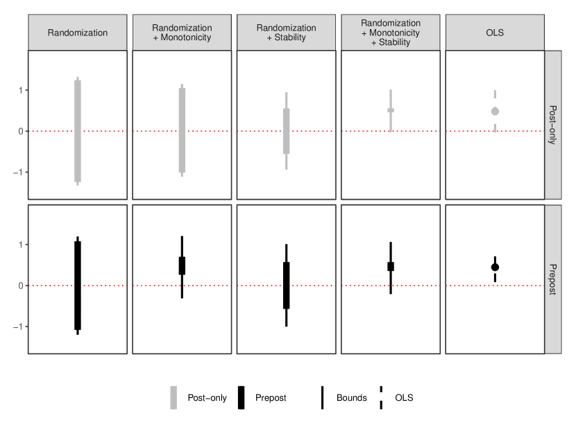
Figure 2: Comparing non-parametric bounds under different assumptions

Notes: The figure shows nonparametric bounds under different sets of assumptions applied to either the post-only data (grey) or the combined pre-post data (black). The thick bars denote the width of the bounds, and thinner lines denote the 95% confidence intervals around the bounds. This estimate included no covariates to facilitate comparison with the nonparametric bounds. For the final panel (“OLS”), the thin lines with dots denote the OLS estimate and 95% confidence interval.

Figure 2 displays the non-parametric bounds (with 95% confidence intervals) for $\delta$ under different sets of assumptions applied to the post-only data (in grey) and to the combined pre-post data (in black). We also include the naïve OLS estimate with 95% confidence interval for comparison in the final panel.

Assuming only randomization, the nonparametric bounds are not informative of the sign of $\delta$, and are much wider than the confidence interval of the naïve OLS estimate. Without incorporating information from covariates or imposing substantive assumptions, there is little evidence for the theorized interaction, where respondents who are land insecure respond more positively to land-based appeals by politicians. Adding the assumption of monotonicity reduces the width of the bounds, especially on the combined pre-post data.

Adding the assumption of stability tightens the bounds to a similar degree for the post-only and pre-post data. With all three assumptions (randomization, monotonicity, and stability), the width of the nonparametric bounds is roughly similar to the width of the confidence intervals around the naïve OLS estimate.

Thus, while the original authors correctly noted that the average treatment effect on the post-measured moderator is insignificant and close to zero, this is not sufficient to ensure that the naïve OLS estimate of the treatment-moderator interaction is free from post-treatment bias. In addition, the observed data cannot rule out the possibility of priming bias for the CATE. With only the design-based assumption of randomization, the nonparametric bounds do not support the hypothesis of a positive interaction effect. It is only with two additional substantive assumptions – monotonicity and stability – that the sharp bounds produce results qualitatively similar to the naïve OLS estimate, of a positive interaction effect that is verging on statistical significance at the 5% confidence level.

5.3 Implementing the sensitivity analysis

While we cannot directly observe the degree of individual-level post-treatment bias, it is possible to investigate how the nonparametric bounds change by varying an assumption about the degree to which this bias is present in the sample. Here, we apply the sensitivity analysis described in Section 4.3.2 to our empirical example. Recall that the parameter $\gamma$ bounds the proportion of respondents who would respond differently to the land insecurity question if asked pre- or post-treatment, and that the minimum feasible value of $\gamma$ is given by $|Q_{11}-Q_{01}|$.

Figure 3 shows how the nonparametric bounds vary as a function of $\gamma$. In this example, we impose Assumptions 3 (monotonicity) and 4 (stability). While $\gamma$ can theoretically range up to 1, here we limit it to 0.5 to aid presentation since the bounds quickly stabilize. The black lines denote the upper and lower bounds, and the shaded ribbon denotes the 95% confidence intervals around the bounds. The lower bound crosses 0 when $\gamma=0.07$: that is, when no more than 7% of respondents are affected by the post-treatment measurement of the moderator. When we incorporate the estimation uncertainty, we can see that the shaded ribbon already includes 0 even for the minimum possible value of $\gamma$ consistent with the observed data (0.02). The sensitivity analysis shows that the sharp bounds are highly sensitive to changes in the degree of post-treatment bias for small values of $\gamma$.

To interpret this sensitive analysis, researchers will need to draw on their substantive knowledge to assess the plausible range of $\gamma$. For example, in this case we may assume that some respondents experience such a high degree of land security that they are unlikely to change their response from “very secure” to “not at all secure” due to post-test measurement. If any respondents are affected by the post-test measurement, it is likely to be those who would respond “somewhat secure” in the pre-test and would change their answer to “not at all secure” in the post-test.

We can estimate the true distribution of the moderator using the pre-test data, in which about 30% of respondents choose the middle category (“somewhat secure”). Out of those respondents, about 40% also reported that they had personally been affected by prior ethnic conflict. Therefore, we might assume that this subset, which comprises about 12% of the full sample, is most likely to be affected by the cueing mechanism and change their perceived land insecurity when measured after treatment. While it may seem like a relatively minor problem if only 12% of the sample is affected, our sensitivity analysis shows that the nonparametric bounds would be about eight times wider ($[-1.02,1.14]$) compared to the case where $\gamma$ is at its minimum ($[0.38,0.64]$).

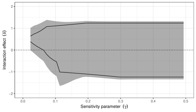
Figure 3: Sensitivity Analysis under Limited Effects on the Moderator

Notes: The figure shows nonparametric bounds (black lines) with 95% confidence intervals (grey ribbon) as a function of $\gamma$, the proportion of respondents whose value of the moderator variable (land insecurity) is affected by post-test measurement. The assumptions of monotonicity and stability are both imposed. While $\gamma$ can vary up to 1, we limit the maximum to 0.5 to aid presentation since the bounds plateau beyond this point.

6 Concluding Remarks

This paper addresses a central tension in survey methodology: how should researchers weigh up priming bias versus post-treatment bias when designing a survey experiment? We provide sharp bounds for interactions for covariates measured post-treatment and show how these bounds vary under additional substantive assumptions. We also provide sensitivity analyses for both types of bias by varying the proportion of respondents whose moderator value changes in the post-test design and the proportion of respondents for whom the pre-test measurement of the moderator would prime their responses. We demonstrate how these tools can be used to diagnose and assess the severity of post-treatment bias and priming bias by applying them to a survey experiment regarding the effect of land-based appeals by politicians on electoral support in Kenya.

Open questions remain from our approach here. In particular, future work could optimize the random placement design to balance the priming and post-treatment bias concerns. In addition, it would be interesting to consider how integrating separate pre-test surveys, often given weeks or months before treatment, might allow for a different set of plausible assumptions and identification.

Appendix A Proofs

A.1 Randomization bounds

Proof of Proposition 1.

Under Assumption 2, the information about the parameter of interest comes from $P_{t}=\mathbb{P}(Y_{i}=1\mid T_{i}=t,Z_{i}=1)$ alone. This is because the distribution of the post-test moderators provides no information about the pre-test moderator. Recall that

$$P_{t}=\pi_{t1}Q_{*}+\pi_{t0}(1-Q_{*}),$$ (10)

where $\pi_{tm}=\mathbb{P}[Y_{i}(t,1)=1\mid M^{*}_{i}=m]$ and $Q_{*}=\mathbb{P}[M^{*}_{i}=1]$.

Below, we show how to derive the upper bound for $\delta$. The derivation of the lower bound is similar. Conditional on $Q_{*}$, we can define the following linear program:

$$\max \pi_{11}-\pi_{01}-\pi_{10}+\pi_{00}$$

subject to $$\pi_{t1}Q_{*}+\pi_{t0}(1-Q_{*})=P_{t}\quad\text{for }t=0,1,$$

$$0\leq\pi_{tm}\leq 1\quad\forall(t,d)\in\{0,1\}^{2}$$

We can convert this to an augmented form by adding slack variables,

$$\max \pi_{11}-\pi_{01}-\pi_{10}+\pi_{00}$$

subject to $$\pi_{t1}Q_{*}+\pi_{t0}(1-Q_{*})=P_{t}\quad\text{for }t=0,1$$

$$\pi_{tm}+s_{tm}=1\quad\forall(t,m)\in\{0,1\}^{2}$$

$$\{\pi_{11},\pi_{01},\pi_{10},\pi_{00},s_{11},s_{01},s_{10},s_{00}\}\geq 0.$$

The feasibility of various basic solutions here will depend on the relationship between the observed probabilities and $Q_{*}$. In Table SM.1, we show basic feasible solutions for the four different conditions relating $P_{1}$ and $P_{0}$ to $Q_{*}$. Under each condition, it is straightforward to determine that the basic feasible solution is also optimal since there is no entering variable that can increase the value of the quantity of interest. Thus, we know that

$$\delta\leq\min\left\{\frac{1+P_{1}-P_{0}}{Q_{*}},\ \frac{1-P_{1}+P_{0}}{1-Q_{*}},\ \frac{1-P_{0}}{Q_{*}}+\frac{1-P_{1}}{1-Q_{*}},\ \frac{P_{1}}{Q_{*}}+\frac{P_{0}}{1-Q_{*}}\right\}$$

Table SM.1: Optimal solutions to the linear program under different conditions

Condition	$\pi_{11}$	$\pi_{10}$	$\pi_{01}$	$\pi_{00}$	$s_{11}$	$s_{01}$	$s_{10}$	$s_{00}$	Value
$P_{1}>Q_{*},P_{0}>1-Q_{*}$	$\frac{P_{1}}{Q_{*}}$	0	0	$\frac{P_{0}}{1-Q_{*}}$	$1-\frac{P_{1}}{Q_{*}}$	1	1	$1-\frac{P_{0}}{1-Q_{*}}$	$\frac{P_{1}}{Q_{*}}+\frac{P_{0}}{1-Q_{*}}$
$P_{1}<Q_{*},P_{0}>1-Q_{*}$	$1$	$\frac{P_{1}-Q_{*}}{1-Q_{*}}$	0	$\frac{P_{0}}{1-Q_{*}}$	$0$	1	1	$1-\frac{P_{0}}{1-Q_{*}}$	$\frac{1-P_{1}+P_{0}}{1-Q_{*}}$
$P_{1}>Q_{*},P_{0}<1-Q_{*}$	$\frac{P_{1}}{Q_{*}}$	0	$\frac{P_{0}-1+Q_{*}}{Q_{*}}$	$1$	$1-\frac{P_{1}}{Q_{*}}$	1	1	$0$	$\frac{P_{1}-P_{0}+1}{Q_{*}}$
$P_{1}<Q_{*},P_{0}<1-Q_{*}$	$1$	$\frac{P_{1}-Q_{*}}{1-Q_{*}}$	$\frac{P_{0}-1+Q_{*}}{Q_{*}}$	$1$	$0$	1	1	$0$	$\frac{1-P_{1}}{1-Q_{*}}+\frac{1-P_{0}}{Q_{*}}$

A similar derivation shows that

$$\delta\geq\max\left(-\frac{1-P_{1}+P_{0}}{Q_{*}},\ -\frac{1+P_{1}-P_{0}}{1-Q_{*}},\ -\frac{P_{0}}{Q_{*}}-\frac{P_{1}}{1-Q_{*}},\ -\frac{1-P_{1}}{Q_{*}}-\frac{1-P_{0}}{1-Q_{*}}\right).$$

Taking a look at these bounds, suppose that $P_{1}\geq 1-P_{0}$, then the upper bound as a function of $Q_{*}$ is:

$$U(Q_{*})=\begin{cases}\frac{P_{0}+(1-P_{1})}{1-Q_{*}}&\text{if}\;Q_{*}\leq 1-P_{0}\\ \frac{1-P_{0}}{Q_{*}}+\frac{1-P_{1}}{1-Q_{*}}&\text{if}\;Q_{*}\in[1-P_{0},P_{1}]\\ \frac{P_{1}+(1-P_{0})}{Q_{*}}&\text{if}\;Q_{*}\geq P_{1}\end{cases}$$

Notice that the numerators of all these functions are positive, so the first bounding function $(P_{0}+1-P_{1})/(1-Q_{*})$ is montonically increasing over its range and the third, $(P_{1}+(1-P_{0}))/Q_{*}$ is monotonically decreasing over its range. Finally, inspection of the middle bounding function shows that it is convex over its range. This implies that the this function must have its maximum at one of the bound points, $1-P_{0}$ or $P_{1}$. Taking the maximum of these two values, and comparing them to the maximum two values from the situation when $P_{1}\leq 1-P_{0}$ gives the expression of the bounds in the result. A similar approach applies to the lower bounds as well.

Sharpness of these bounds is implied by the linear nature of the optimization function and the convexity of the feasible set. If these bounds were not sharp, this would imply that that there are bounds sharper than these that contain all values of $\delta$ consistent with the data and maintained assumptions. But this is clearly contradicted by the fact that the solutions in Table SM.1 are feasible and would fall outside these supposedly sharper bounds. ∎

A.2 Bounds under additional assumptions

To derive bounds under additional assumptions, we first derive bounds conditional on the strata probabilities.

Lemma SM.1.

The bounds on $\delta$ for given values of $\bm{\rho}$ are $\delta\in[\delta_{L}(\bm{\rho}),\delta_{U}(\bm{\rho})]$, where

$$\delta_{U}(\bm{\rho}) =P_{111}\left(\frac{Q_{11}}{Q_{*}}\right)-P_{011}\left(\frac{Q_{01}}{Q_{*}}\right)-P_{110}\left(\frac{1-Q_{11}}{1-Q_{*}}\right)+P_{010}\left(\frac{1-Q_{01}}{1-Q_{*}}\right)$$

$$+\frac{1}{Q_{*}(1-Q_{*})}\min\left\{\begin{matrix}P_{110}(1-Q_{11})\\ \rho_{011}+\rho_{001}\\ Q_{*}-P_{111}Q_{11}\end{matrix}\right\}+\frac{1}{Q_{*}(1-Q_{*})}\min\left\{\begin{matrix}P_{011}Q_{01}\\ \rho_{110}+\rho_{010}\\ 1-Q_{*}-P_{010}(1-Q_{01})\end{matrix}\right\},$$

and,

$$\delta_{L}(\bm{\rho}) =P_{111}\left(\frac{Q_{11}}{Q_{*}}\right)-P_{011}\left(\frac{Q_{01}}{Q_{*}}\right)-P_{110}\left(\frac{1-Q_{11}}{1-Q_{*}}\right)+P_{010}\left(\frac{1-Q_{01}}{1-Q_{*}}\right)$$

$$+\frac{1}{Q_{*}(1-Q_{*})}\max\left\{\begin{matrix}-P_{111}Q_{11}\\ -\rho_{110}-\rho_{100}\\ -1+Q_{*}+P_{110}(1-Q_{11})\end{matrix}\right\}+\frac{1}{Q_{*}(1-Q_{*})}\max\left\{\begin{matrix}-P_{011}Q_{01}\\ -\rho_{001}-\rho_{101}\\ -Q_{*}+P_{011}Q_{01}\end{matrix}\right\}.$$

Proof.

Conditional on $\rho_{s}$ and $Q_{*}$, deriving the bounds on $\delta$ is a standard linear programming problem. We now describe the process for deriving these bounds at a general level. Without any assumptions, we are interested in maximizing or minimizing the objective function,

$$\delta= P_{111}\left(\frac{Q_{11}}{Q_{*}}\right)-P_{011}\left(\frac{Q_{01}}{Q_{*}}\right)-P_{110}\left(\frac{1-Q_{11}}{1-Q_{*}}\right)+P_{010}\left(\frac{1-Q_{01}}{1-Q_{*}}\right)$$

$$+\mu_{011}(1,1)\frac{\rho_{011}}{Q_{*}(1-Q_{*})}+\mu_{001}(1,1)\frac{\rho_{001}}{Q_{*}(1-Q_{*})}$$

$$-\mu_{110}(1,1)\frac{\rho_{110}}{Q_{*}(1-Q_{*})}-\mu_{100}(1,1)\frac{\rho_{100}}{Q_{*}(1-Q_{*})}$$

$$+\mu_{110}(0,1)\frac{\rho_{110}}{Q_{*}(1-Q_{*})}+\mu_{010}(0,1)\frac{\rho_{010}}{Q_{*}(1-Q_{*})}$$

$$-\mu_{101}(0,1)\frac{\rho_{101}}{Q_{*}(1-Q_{*})}-\mu_{001}(0,1)\frac{\rho_{001}}{Q_{*}(1-Q_{*})},$$

subject to the constraints

$$P_{111}Q_{11} =\mu_{111}(1,1)\rho_{111}+\mu_{101}(1,1)\rho_{101}+\mu_{110}(1,1)\rho_{110}+\mu_{100}(1,1)\rho_{100}$$

$$P_{011}Q_{01} =\mu_{111}(0,1)\rho_{111}+\mu_{011}(0,1)\rho_{011}+\mu_{110}(0,1)\rho_{110}+\mu_{010}(0,1)\rho_{010}$$

$$P_{110}(1-Q_{11}) =\mu_{011}(1,1)\rho_{011}+\mu_{110}(1,1)\rho_{110}+\mu_{010}(1,1)\rho_{010}+\mu_{000}(1,1)\rho_{000}$$

$$P_{010}(1-Q_{01}) =\mu_{101}(0,1)\rho_{101}+\mu_{001}(0,1)\rho_{001}+\mu_{100}(0,1)\rho_{100}+\mu_{000}(0,1)\rho_{000}$$

$$0 \leq\mu_{s}(t)\leq 1,\quad\forall s,t.$$

For this step, we do not need to specify constraints on $\rho_{s}$ because we consider them fixed (and $Q_{*}$ is a linear function of $\rho_{s}$). The simplex tableau method yields the given bounds. ∎

Proof of Proposition 2.

Recall the constraints on the strata probabilities:

$$Q_{11} =\rho_{111}+\rho_{101}+\rho_{110}+\rho_{100}$$

$$Q_{01} =\rho_{111}+\rho_{011}+\rho_{110}+\rho_{010}$$

$$Q_{*} =\rho_{111}+\rho_{011}+\rho_{101}+\rho_{001},$$

Under monotonicity, we only have strata $S_{i}\in\{111,110,010,100,000\}$, so we have $Q_{*}=\mathbb{P}[M^{*}_{i}=1]=\rho_{111}$ and $\rho_{110}+\rho_{010}=Q_{01}-Q_{*}$ and $\rho_{110}+\rho_{100}=Q_{11}-Q_{*}$. Plugging these values into the bounds from Lemma SM.1, we obtain

$$\delta_{U}(Q_{*}) =P_{111}\left(\frac{Q_{11}}{Q_{*}}\right)-P_{011}\left(\frac{Q_{01}}{Q_{*}}\right)-P_{110}\left(\frac{1-Q_{11}}{1-Q_{*}}\right)+P_{010}\left(\frac{1-Q_{01}}{1-Q_{*}}\right)$$

$$+\frac{1}{Q_{*}(1-Q_{*})}\min\left\{\begin{matrix}P_{110}(1-Q_{11})\\ 0\\ Q_{*}-P_{111}Q_{11}\end{matrix}\right\}+\frac{1}{Q_{*}(1-Q_{*})}\min\left\{\begin{matrix}P_{011}Q_{01}\\ Q_{01}-Q_{*}\\ 1-Q_{*}-P_{010}(1-Q_{01})\end{matrix}\right\},$$

and,

$$\delta_{L}(Q_{*}) =P_{111}\left(\frac{Q_{11}}{Q_{*}}\right)-P_{011}\left(\frac{Q_{01}}{Q_{*}}\right)-P_{110}\left(\frac{1-Q_{11}}{1-Q_{*}}\right)+P_{010}\left(\frac{1-Q_{01}}{1-Q_{*}}\right)$$

$$+\frac{1}{Q_{*}(1-Q_{*})}\max\left\{\begin{matrix}-P_{111}Q_{11}\\ -Q_{11}-Q_{*}\\ -1+Q_{*}+P_{110}(1-Q_{11})\end{matrix}\right\}+\frac{1}{Q_{*}(1-Q_{*})}\max\left\{\begin{matrix}-P_{011}Q_{01}\\ 0\\ -Q_{*}+P_{011}Q_{01}\end{matrix}\right\}.$$

We further simplify the upper bound expression by noting that $P_{110}(1-Q_{11})\geq 0$ and $Q_{01}-Q_{*}\leq 1-Q_{*}-P_{010}(1-Q_{01})$. The lower bound simplifies because $Q_{11}-Q_{*}\leq 1-Q_{*}-P_{110}(1-Q_{11})$ and $P_{011}Q_{01}\geq 0$. Removing these extraenous conditions gives the result in the text.

∎

Proof of Proposition 3.

Under the maintained assumptions, $Q_{*}=Q_{01}$, which we plug into the expression of Proposition 2. Then, the result is immediate upon noting that $P_{011}Q_{01}-Q_{01}\leq 0$, $P_{011}Q_{01}\geq 0$ and rearranging terms. ∎

For calculating the bounds under the sensitivity constraints, we can take the bounds from Lemma SM.1 and solve a corresponding linear programming problem to optimize them with respect to the principal strata probabilities. For example, depending the observed data, the upper bound will depend on $\rho_{011}+\rho_{001}$, $\rho_{110}+\rho_{010}$, or $\rho_{011}+\rho_{001}+\rho_{110}+\rho_{010}$. To find the upper bound across values of $\bm{\rho}$, we apply the linear programming machinery to finding the upper bound for each of these quantities subject to the constraints that

$$Q_{11} =\rho_{111}+\rho_{101}+\rho_{110}+\rho_{100}$$

$$Q_{01} =\rho_{111}+\rho_{011}+\rho_{110}+\rho_{010}$$

$$Q_{*} =\rho_{111}+\rho_{011}+\rho_{101}+\rho_{001},$$

where $0\leq\rho_{s}\leq 1$ for all $s$ and $\sum_{s\in\mathcal{S}}\rho_{s}=1$. Note that for the sensitivity analysis, we may impose additional constraints on $\rho_{s}$ in this step. As an example, for the objection function of $\rho_{011}+\rho_{001}$, we have the upper bound

$$\min\left\{1-Q_{11},Q_{*},1-Q_{01}+Q_{*},\frac{1}{2}(1-Q_{11}+Q_{*}),1+Q_{01}-Q_{11}\right\}.$$

Plugging these bounds into the upper bound $\delta_{U}(\bm{\rho})$ will yield an upper bound purely as a function of observed parameters and $Q_{*}$ and $\gamma$ ( the sensitivity parameter). Under some of our assumptions, inspection of the resulting functions reveals that the maximum of these functions can only occur at a handful of critical values of $Q_{*}$ which can be evaluated and compared quickly. Otherwise, we use a standard optimization routine to find the value of $Q_{*}$ that maximizes the upper bound or minimizes the lower bound.

Appendix B Parametric Bayesian Approach to Incorporate Covariates

The nonparametric bounds above are sharp in the sense that they leverage all information about the outcome, moderator, treatment, and question order. Researchers, however, often have additional data in the form of covariates that may help reduce the uncertainty of their estimates. Here, we consider a Bayesian parametric model of the principal strata approach to the pre-test, post-test, and random placement designs, building on the work of Mealli and Pacini (2013) (see also Imbens and Rubin, 1997; Hirano et al., 2000). Unlike the nonparametric bounds approach, a Bayesian model allows us to incorporate prior information about the data-generating process in a smooth and flexible manner.

B.1 The Model

Our approach focuses on a data augmentation strategy that models the joint distribution of the outcomes and the principal strata, the latter of which are not directly observable. We allow the distribution of the potential outcomes and principal strata conditional on those strata to further depend on covariates via a binomial and multinomial logistic model, respectively:

$$\mathbb{P}(Y_{i}=1\mid T_{i}=t,Z_{i}=z,S_{i}=s,\bm{X}_{i}) =\mu_{is}(t,z)=\textrm{logit}^{-1}(\alpha_{tz|s}+\mathbold{X}^{\prime}_{i}\mathbold{\beta}),$$

$$\mathbb{P}(S_{i}=s\mid\mathbold{X}_{i}) =\rho_{is}=\frac{\exp(\mathbold{X}^{\prime}_{i}\mathbold{\psi}_{s})}{\sum_{j\in\mathcal{S}}\exp(\mathbold{X}^{\prime}_{i}\mathbold{\psi}_{j})},$$

where $\mathbold{X}_{i}$ denotes observed pre-treatment covariates that might be predictive of unit $i$’s outcome and principal strata. Note that the strata probabilities do not depend on $T_{i}$ and $Z_{i}$ due to randomization. We gather the parameters as $\mathbold{\alpha}=\{\alpha_{tz|s}\}$ and $\mathbold{\psi}=\{\mathbold{\psi}_{s}\}$. We can easily incorporate assumptions like monotonicity and stable moderators by simply restricting the space of possible principal strata $\mathcal{S}$.

Our goal is to make inferences about the posterior distribution of these parameters and the ultimate quantities of interest, $\tau(d)$ and $\delta$. There are two ways to represent these quantities under this parametric model, resulting in two different types of posterior distributions. The first is based on population inference and derives expressions for $\tau(d)$ and $\delta$ purely in terms of the parameters of the model. The second is based on in-sample inference and derives expressions for $\tau(d)$ and $\delta$ in terms of potential outcomes in a particular sample.

For the population inference approach, we first note that due to consistency and randomization, we have $\mu_{is}(t,z)=\mathbb{P}(Y_{i}(t,z)=1\mid S_{i}=s,\mathbold{X}_{i})$. Thus, we can write the values of the quantities of interest for a given unit as,

$$\tau_{i}(m)=\mathbb{E}\left[Y^{*}_{i}(1)-Y^{*}_{i}(0)\mid M^{*}_{i}=m,X_{i}\right]\ =\ \sum_{s\in\mathcal{S}^{*}_{d}}(\mu_{is}(1,1)-\mu_{is}(0,1))\rho_{is},$$

and $\delta_{i}=\tau_{i}(1)-\tau_{i}(0)$, where we omit the implied dependence on $(\mathbold{\alpha,\beta,\psi})$ and remember that $\mathcal{S}^{*}_{d}$ is the set of strata levels such that $M^{*}_{i}=m$, for $m\in\{0,1\}$. Using the empirical distribution of covariates, the average of these conditional mean differences and interactions will equal the overall quantities of interest, i.e., $\tau(m)=\sum_{i=1}^{n}\tau_{i}(m)/n$ and $\delta=\sum_{i=1}^{n}\delta_{i}/n$.

The in-sample versions of the quantities of interest are more straightforward, since they are simply the conditional mean differences and interaction among the units in the sample,

$$\tau_{s}(m)=\frac{\sum_{i=1}^{n}\mathbb{I}(M^{*}_{i}=m)\left\{Y^{*}_{i}(1)-Y^{*}_{i}(0)\right\}}{\sum_{i=1}^{n}\mathbb{I}(M^{*}_{i}=m)},$$

and $\delta_{s}=\tau_{s}(1)-\tau_{s}(0)$. Obviously, across repeated samples, we can relate these to the population quantities as $\mathbb{E}[\tau_{s}(m)]=\tau(m)$ and $\mathbb{E}[\delta_{s}]=\delta$.

We develop an efficient Markov Chain Monte Carlo (MCMC) algorithm to take draws from the posterior and then calculate these quantities of interest. Our Gibbs sampler can also be simplified and used for inference in the absence of pre-treatment covariates, which can be viewed as a Bayesian alternative to uncertainty estimation for the partially identified parameters discussed in Section 4.3.3. We provided details of these algorithms in Supplemental Materials C.

This Bayesian approach has the advantage of easily incorporating covariates, but it does require us to select prior distribution for the model parameters, some of which are unidentified in the frequentist sense. Thus, the identification of these parameters will depend on the prior. To investigate this, we take draws of the prior predictive distribution under different prior structures, which we show in Figure SM.4. All the priors we considered are symmetric, but uniform priors on the model parameters lead to somewhat informative priors on the ultimate quantity of interest. Thus, we rely on more dispersed priors for the simulations and the application. We discuss the choice of prior distribution more fully in Supplemental Materials C.

We conduct two simulation studies to demonstrate the gains in efficiency from the monotonicity and stability assumptions and the incorporation of covariates in the Bayesian approach. The first simulation varies the assumptions of the data-generating process and compares the posterior variance of these distributions across combinations of our two assumptions. The second simulation varies the predictive power of the covariates on the outcome and the strata in the data-generating process and compares the variance of the posterior distributions from Gibbs run on each simulated data set with and without incorporating covariates. We present these results in Supplemental Materials  C.1.

Appendix C MCMC Algorithm

In this section we describe our MCMC algorithm for the Bayesian model of Section B. Our goal is to sample from the joint distribution of the parameters and the principal strata indicator,

$$\mathbb{P}(\mathbold{\alpha,\beta,\psi},\mathbold{S} \mid\mathbold{Y},\mathbold{X,T,Z,M})\propto$$

$$\prod_{i=1}^{n} \left(\sum_{s\in\mathcal{S}_{i}}\left[\mathbb{P}(Y_{i}\mid T_{i},Z_{i},S_{i}=s,\bm{X}_{i})\mathbb{P}(S_{i}=s\mid\mathbold{X}_{i})\right]^{\mathbb{I}(S_{i}=s)}\right)\mathbb{P}(\mathbold{\alpha,\beta,\psi}),$$

where $\mathcal{S}_{i}=\mathcal{S}(T_{i},Z_{i},M_{i})$ are the set of principal strata to which unit $i$ could possibly belong. When the set of observed pre-treatment covariates ($\bm{X}_{i}$) is empty, the parameter space reduces to that of a standard finite mixture model, and sampling from the joint posterior is straightforward. With $\bm{X}_{i}$, Bayesian inference for the model is more complicated. Traditionally, Bayesian inference for logistic regression models has been challenging due to a lack of a simple Gibbs sampling algorithm. Recently, however, Polson, Scott and Windle (2013) introduced a simple data-augmentation strategy based on the Pólya-Gamma (PG) distribution, obviating the need for approximate methods or precise tuning of a Metropolis-Hastings algorithm. We use this approach for both the binary and multinomial logistic regression models for the outcome and principal strata, respectively. This allows a simple Gibbs structure where the full conditional posterior distributions of $(\mathbold{\alpha,\beta})$ and $\mathbold{\psi}$ are Normal conditional on specific draws from the PG distribution.

Conditional on the other parameters, then the full conditional posterior of the principal strata follows a similar form to Hirano et al. (2000),

$$\mathbb{P}(S_{i}=s\mid Y_{i},\mathbold{X}_{i},T_{i},Z_{i},M_{i},\mathbold{\alpha,\beta,\psi})=\frac{\mu_{is}(T_{i},Z_{i})^{Y_{i}}(1-\mu_{is}(T_{i},Z_{i}))^{1-Y_{i}}\rho_{is}}{\sum_{k\in\mathcal{S}_{i}}\mu_{ik}(T_{i},Z_{i})^{Y_{i}}(1-\mu_{ik}(T_{i},Z_{i}))^{1-Y_{i}}\rho_{ik}},$$

where we suppress the dependence of $\mu_{is}$ and $\rho_{is}$ on the model parameters. Repeatedly drawing from these full conditional posterior distributions should provide a sample from the above joint posterior and allow for posterior inference in the usual manner. In each iteration, $r\in\{1,\ldots,R\}$, of the algorithm, we have draws

$$\left(\left\{\widehat{S}_{i}^{(r)}\right\}_{i=1}^{n},\widehat{\mathbold{\psi}}^{(r)},\widehat{\mathbold{\alpha}}^{(r)},\widehat{\mathbold{\beta}}^{(r)}\right).$$

We can use these draws to generate draws of the population and in-sample versions of the quantity of interest. Given that $\widehat{S}^{(r)}_{i}$ is the imputed principal strata imputed for unit $i$ in the $r$th draw from the posterior, we let

$$\widehat{\mu}^{(r)}_{i}(t,z)=\widehat{\mu}_{i,\widehat{S}^{(r)}_{i}}(t,z,\widehat{\mathbold{\alpha}}^{(r)},\widehat{\mathbold{\beta}}^{(r)})$$

be the mean of the potential outcomes conditional on that imputed principal strata. Furthermore, let $\widehat{\rho}^{(r)}_{is}$ be the $r$th draw of the predicted probabilities of each principal strata for each unit. Then, we can calculate the population quantity as

$$\widehat{\delta}_{p}^{(r)}=\frac{1}{n}\sum_{i=1}^{n}\left(\sum_{s\in\mathcal{S}^{*}_{1}}(\widehat{\mu}^{(r)}_{is}(1,1)-\widehat{\mu}^{(r)}_{is}(0,1))\widehat{\rho}^{(r)}_{is}\right)-\left(\sum_{s\in\mathcal{S}^{*}_{0}}(\widehat{\mu}^{(r)}_{is}(1,1)-\widehat{\mu}^{(r)}_{is}(0,1))\widehat{\rho}^{(r)}_{is}\right),$$

For the in-sample quantity, we can then draw imputed values of the missing potential outcomes themselves $\widehat{Y}^{*,(r)}_{i}(1)\sim\text{Bin}(\widehat{\mu}^{(r)}_{i}(1,1))$ and $\widehat{Y}^{*,(r)}_{i}(0)\sim\text{Bin}(\widehat{\mu}^{(r)}_{i}(0,1))$. We can combine this with the imputed value of $M^{*}_{i}$, which mechanically derives from $\widehat{S}_{i}^{{r}}$, to get the $r$th draw from the posterior of $\delta_{s}$,

$$\widehat{\delta}^{(r)}_{s}=\frac{\sum_{i=1}^{n}\widehat{M}^{*,(r)}_{i}\left\{\widehat{Y}^{*,(r)}_{i}(1)-\widehat{Y}^{*,(r)}_{i}(0)\right\}}{\sum_{i=1}^{n}\widehat{M}^{*,(r)}_{i}}-\frac{\sum_{i=1}^{n}\left(1-\widehat{M}^{*,(r)}_{i}\right)\left\{\widehat{Y}^{*,(r)}_{i}(1)-\widehat{Y}^{*,(r)}_{i}(0)\right\}}{\sum_{i=1}^{n}\left(1-\widehat{M}^{*,(r)}_{i}\right)}.$$

Broadly speaking, we would not expect very large differences between these two targets, except for slightly less posterior variance for the in-sample version.

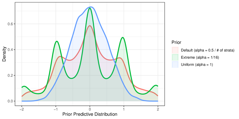
Figure SM.4: Prior predictive distribution of the parameter under three different prior distributions: (red) the default priors that scales a Jeffreys prior by the number of principal strata; (blue) a uniform prior on all parameters; and (green) a more extreme prior that has $\alpha=1/16$.

As discussed in the main text, the priors need careful attention because they drive the identification of the parameters that are unidentified by the likelihood. One additional complication comes from how the ultimate quantity of interest is a function of the parameters so we cannot directly place, for example, a uniform prior on $\delta$. Figure SM.4 shows the prior predictive distribution for interaction with three different priors when monotonicity and stable moderator under control are assumed and there are no covariates. The uniform prior on all parameters results in a prior on $\delta$ that has more density in the center of identified range than we might expect. This result is similar to how sums of uniform random variables are not themselves uniform. We can counteract this issue by reducing the Dirichlet and Beta hyperparameters below 1 to put more density at extreme values of the parameters compared to the center. Dropping these parameters down to 1/16 (in green) leads to more mass on strata means closer to 0 or 1 and strata probabilities closer to 0 and 1. In terms of the interaction, this leads to more mass at the values -2, -1, 0, 1, and 2. Our default prior (red) is one that scales the hyperparameters by the inverse of the number of strata to achieve something closer to a uniform distribution.

Additionally, we re-ran the Gibbs empirical analysis of the Horowitz and Klaus (2020) study, adjusting the priors to the extreme values or uniform values in the previous simulation. The results are displayed in Figure SM.5, demonstrating the general consistency of the point estimates across starting priors, although there is some fluctuations in the variance of the results.

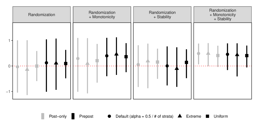
Figure SM.5: Comparing Bayesian estimates for $\delta$ for default, extreme, and uniform priors

Notes: Figure shows posterior means and 95% credible intervals for $\delta$ under different sets of assumptions, applied to either the post-only data (grey) or the combined pre-post data (black). Estimates are shown with default, extreme, and uniform priors, (denoted by circles, triangles, and squares, respectively). We follow the original authors in using age, gender, education, and closeness to one’s ethnic group as covariates. The naïve OLS estimates are included for comparison.

C.1 Simulation Evidence for the Bayesian Approach

Simulation Study I.

In the first simulation study, we generate simulated data with $n=1000$ constructed using a data generating process that matches the Bayesian posterior, pre-specifying coefficient values for the outcome and principal strata models, randomly drawing values of $Z$, $T$, and three covariates $X_{1}$, $X_{2}$, and $X_{3}$, and generating values of $Y$ and $M$ from the models. Tables SM.2 and SM.3 in the Supplemental Materials display the $\beta$ coefficients for the outcome and $\psi$ coefficients for the for the true data generating process (DGP). The DGP assumes that monotonicity and stable moderator under control both hold so that there are three feasible strata ($\mathcal{S}=\{000,100,111\}$). Thus, in this setting it would be most appropriate to incorporate both assumptions into the MCMC algorithm for sampling from the posterior distribution. Since these assumptions narrow the nonparametric bounds, we expect the assumptions to reduce variance of the posterior distribution of $\delta$.

To test this, we perform a Monte Carlo simulation with 1,000 iterations. For each iteration, we calculate the posterior distribution of $\delta$ with the same data across four different versions of the MCMC algorithm: enforcing just the monotonicity assumption, enforcing just the stable moderator under control assumption, enforcing neither assumption, and enforcing both assumptions. Each run of our MCMC algorithm consists of 4 chains with 2,000 iterations each, 200 burn-in (or warm-up) iterations, and a thinning parameter of 2. Both in-sample and population $\delta$ values are calculated at each iteration and the variance of the posterior is calculated from a sample of 1,000 draws from the posterior. This is done for each of the 1,000 simulated datasets, and for each dataset we compute the percent reduction in variance compared to the MCMC algorithm with no assumptions when using the algorithm with the monotonicity assumption, the stable moderator under control assumption, or both assumptions.

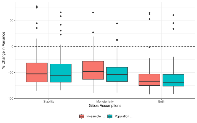
Figure SM.6: Variance reduction from different combinations of assumptions. Boxplots present distribution of % variance reduction of $\delta$ from the MCMC algorithm with the labeled assumptions compared to same algorithm with no assumptions, across 1,000 draws of simulated data. For each simulation iteration, 4 chains were run for each combination of assumptions. MCMC parameters: 2,000 iterations, 200 burn-in, 2 thinning parameter, simulated data $n=1,000$.

Figure SM.6 presents boxplots for the distribution of reductions in variance for each combination of assumptions. Both the monotonicity and stable moderator assumptions on their own reduce the variance compared to no assumptions, while making both assumptions reduces the variance even further. The monotonicity assumption showed a median posterior variance reduction of 40.8% for the in-sample $\delta$ and 42.0% for the population $\delta$. The stable moderator under control assumption on reduced the posterior variance by a median reduction of 47.1% (in-sample $\delta$) and 50.4% (population $\delta$). The MCMC algorithm with both assumptions exhibited a posterior variance reduction of 59.3% (in-sample $\delta$) and 61.7% (population $\delta$).

Simulation Study II.

In the second simulation study, we drew a series of simulated datasets under different conditions where the covariates had a weak, medium, or strong correspondence with the outcome and principal strata in the data generating processes. Thus, there were six total conditions: Weak, Medium, and Strong influence in the outcome DGP; and Weak, Medium, and Strong influence in the principal strata DGP. The values of the coefficients for these conditions are $\beta$ and $\psi$ values of 0, 0.25, and 0.5, respectively. When varying the influence of covariates in the outcome DGP, the influence of covariates on the strata was held constant, and the influence in the outcome model was similarly held constant when varying influence in the strata DGP. Fixed values of the $\beta$’s and $\psi$’s are shown in the Supplemental Materials in Tables SM.4 and SM.5.

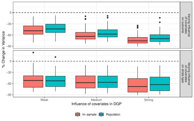
Figure SM.7: Variance reduction from incorporation of covariates. Boxplots present distribution of % variance reduction of $\delta$ from Gibbs with covariates compared to MCMC without covariates, across 1,000 draws of simulated data. For each draw 4 MCMC chains were run for each combination of assumptions. MCMC parameters: 2,000 iterations, 200 burn-in, 2 thinning parameter, simulated data $n=1,000$.

For each condition, we drew 1,000 simulated datasets and ran the MCMC algorithm twice: one time incorporating covariates and one time omitting them. Each MCMC run consisted of the same iterations, burn-in, and thinning parameters as in the previous simulation study. We again calculate in-sample and population $\delta$ values for each iteration of the Gibbs and calculate the variance of the posterior distribution and the % variance reduction comparing the Gibbs with covariates to that without. Figure SM.7 presents boxplots for the distribution in variance reduction. When we vary the influence of covariates on the outcome, we see a clear variance reduction in all conditions, and we observe a larger reduction as the influence of covariates on the outcome in the DGP increases. When testing the impact of incorporating covariates across different levels of influence in the DGP on the strata, the pattern is less pronounced, with overall reduction increases in all conditions but slightly lower reductions in the Medium than Weak condition. The Strong condition still has the largest variance reduction overall, however, so in general the efficiency gains from incorporating covariates are increasing as the influence of covariates on strata in the data increases.

Appendix D Additional Simulation Details

Table SM.2: $\beta$ Values for DGP in Bayesian Assumptions Simulation

Variable	$\beta$
(Intercept)	-2.00
X1	1.00
X2	0.15
X3 (Medium)	0.24
X3 (Large)	0.28
T	0.83
Z	-0.01
T:Z	0.11
S111	0.41
S100	0.62
T:S111	0.01
T:S100	0.23
Z:S111	0.20
Z:S100	-0.02
T:Z:S111	-0.90
T:Z:S100	0.09

Table SM.3: $\psi$ Values for DGP in Bayesian Assumptions Simulation

	S111	s100	s000
(Intercept)	-2.06	-1.00	0.00
X1	2.00	1.50	0.00
X2	0.50	0.17	0.00
X3 (Medium)	1.35	-0.28	0.00
X3 (Large)	1.75	-1.01	0.00

Table SM.4: Fixed $\beta$ Values in Covariate Simulation

Variable	$\beta$
(Intercept)	-1.00
X1	1.00
X2	0.50
X3 (Medium)	0.50
X3 (Large)	0.28
T	0.83
Z	-0.01
T:Z	0.11
S111	0.41
S100	0.62
T:S111	2.00
T:S100	-0.13
Z:S111	0.50
Z:S100	0.10
T:Z:S111	0.05
T:Z:S100	0.01

Table SM.5: Fixed $\psi$ values in Bayesian Covariate Simulation

	S111	S100	S000
(Intercept)	-2.06	-1.00	0.00
X1	2.00	1.50	0.00
X2	0.50	0.17	0.00
X3 (Medium)	1.35	-0.28	0.00
X3 (Large)	1.75	-1.01	0.00

D.1 Comparing the sharp bounds and Bayesian approach without covariates

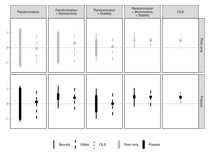
Figure SM.8: Comparing non-parametric bounds and Bayesian estimates for $\delta$ under different assumptions

Notes: The figure shows nonparametric bounds and Bayesian estimates of the quantity of interest under different sets of assumptions applied to either the post-only data (grey) or the combined pre-post data (black). The thick bars denote the width of the bounds, and thinner lines denote the 95% confidence intervals around the bounds. Across the first four panels, the thin lines with dots denote the Bayesian posterior mean and 95% credible interval. This estimate included no covariates to facilitate comparison with the nonparametric bounds. For the final panel (“OLS”), the thin lines with dots denote the OLS estimate and 95% confidence interval.

Figure SM.8 displays the non-parametric bounds (with 95% confidence intervals) and Bayesian estimates (posterior means with 95% credible intervals) for $\delta$ under different sets of assumptions applied to the post-only data (in grey) and to the combined pre-post data (in black). We also include the naïve OLS estimate with 95% confidence interval for comparison in the final panel.

D.2 Incorporating covariates into the Bayesian approach

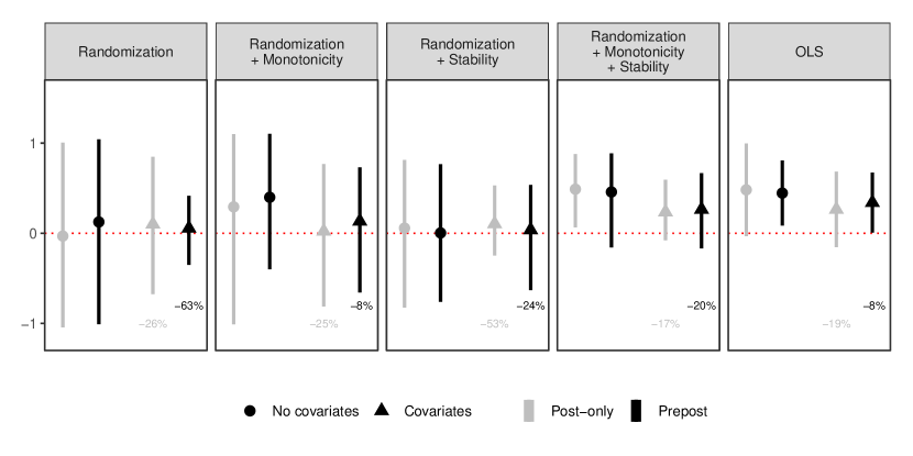
Figure SM.9: Comparing Bayesian estimates for $\delta$ with and without covariates

Notes: Figure shows posterior means and 95% credible intervals for $\delta$ under different sets of assumptions applied to either the post-only data (grey) or the combined pre-post data (black). Estimates are shown with and without the inclusion of covariates (denoted by triangles and circles, respectively), and the numbers indicate the reduction in the width of the credible intervals due to the inclusion of covariates for the post-only data (in grey) and the combined pre-post data (in black). We follow the original authors in using age, gender, education, and closeness to one’s ethnic group as covariates. The naïve OLS estimates are included for comparison.

Thus far, our Bayesian estimates have omitted covariates to aid comparison with the nonparametric bounds. However, as discussed above, a key attraction of the Bayesian approach is the ease with which we can incorporate additional information. Figure SM.9 presents posterior means with 95% credible intervals, both with and without covariates, under different assumptions. We follow the original authors in using age, gender, education, and closeness to one’s ethnic group as covariates. Including covariates significantly tightens the credible intervals, especially when fewer assumptions are imposed. For example, when only randomization is assumed, the width of the 95% credible interval shrinks by more than 50% when including covariates. While including covariates does not alter our substantive conclusions in this case, it does show that incorporating additional information can lead to large gains in precision. Since researchers often include a wide range of control variables in the design of a survey experiment, flexibly leveraging this information is a key advantage of the Bayesian approach.

References

- (1)
- Acharya, Blackwell and Sen (2016) Acharya, Avidit, Matthew Blackwell and Maya Sen. 2016. “Explaining Causal Findings Without Bias: Detecting and Assessing Direct Effects.” American Political Science Review 110(3):512–529.
- Albertson and Jessee (2022) Albertson, Bethany and Stephen Jessee. 2022. “Moderator Placement in Survey Experiments: Racial Resentment and the “Welfare” versus “Assistance to the Poor” Question Wording Experiment.” Journal of Experimental Political Science pp. 1–7. Forthcoming.
- Balke and Pearl (1997) Balke, Alexander and Judea Pearl. 1997. “Bounds on treatment effects from studies with imperfect compliance.” Journal of the American Statistical Association 92:1171–1176.
- Chernozhukov, Lee and Rosen (2013) Chernozhukov, Victor, Sokbae Lee and Adam M. Rosen. 2013. “Intersection Bounds: Estimation and Inference.” Econometrica 81(2):667–737.
- Chong and Druckman (2010) Chong, Dennis and James N. Druckman. 2010. “Dynamic Public Opinion: Communication Effects over Time.” American Political Science Review 104(4):663–680.
- Fang and Santos (2018) Fang, Zheng and Andres Santos. 2018. “Inference on Directionally Differentiable Functions.” The Review of Economic Studies .
- Frangakis and Rubin (2002) Frangakis, Constantine E. and Donald B. Rubin. 2002. “Principal Stratification in Causal Inference.” Biometrics 58(1):21–29.
- Hirano et al. (2000) Hirano, Keisuke, Guido W. Imbens, Donald B. Rubin and Xiao-Hua Zhou. 2000. “Assessing the effect of an influenza vaccine in an encouragement design.” Biostatistics 1(1):69–88.
- Holland (1986) Holland, Paul W. 1986. “Statistics and Causal Inference (with Discussion).” Journal of the American Statistical Association 81:945–960.
- Horowitz and Klaus (2020) Horowitz, Jeremy and Kathleen Klaus. 2020. “Can politicians exploit ethnic grievances? An experimental study of land appeals in Kenya.” Political Behavior 42(1):35–58.
- Horowitz and Manski (2000) Horowitz, Joel L. and Charles F. Manski. 2000. “Nonparametric Analysis of Randomized Experiments with Missing Covariate and Outcome Data.” Journal of the American Statistical Association 95(449):77–84.
- Imai and Yamamoto (2010) Imai, Kosuke and Teppei Yamamoto. 2010. “Causal Inference with Differential Measurement Error: Nonparametric Identification and Sensitivity Analysis.” American Journal of Political Science 54(2):543–560.
- Imbens and Manski (2004) Imbens, Guido W. and Charles F Manski. 2004. “Confidence Intervals for Partially Identified Parameters.” Econometrica 72(6):1845–1857.
- Imbens and Rubin (1997) Imbens, Guido W. and Donald B. Rubin. 1997. “Bayesian inference for causal effects in randomized experiments with noncompliance.” The Annals of Statistics 25(1):305–327.
- Klar (2013) Klar, Samara. 2013. “The influence of competing identity primes on political preferences.” The Journal of Politics 75(4):1108–1124.
- Klar, Leeper and Robison (Forthcoming) Klar, Samara, Thomas J. Leeper and Joshua Robison. Forthcoming. “Studying Identities with Experiments: Weighing the Risk of Post-Treatment Bias Against Priming Effects.” Journal of Experimental Political Science .
- Levis et al. (2023) Levis, Alexander W., Matteo Bonvini, Zhenghao Zeng, Luke Keele and Edward H. Kennedy. 2023. “Covariate-assisted bounds on causal effects with instrumental variables.”.
- Mealli and Pacini (2013) Mealli, Fabrizia and Barbara Pacini. 2013. “Using Secondary Outcomes to Sharpen Inference in Randomized Experiments With Noncompliance.” Journal of the American Statistical Association 108(503):1120–1131.
- Montgomery, Nyhan and Torres (2018) Montgomery, Jacob M., Brendan Nyhan and Michelle Torres. 2018. “How Conditioning on Posttreatment Variables Can Ruin Your Experiment and What to Do about It.” American Journal of Political Science 62(3):760–775.
- Morris, Carranza and Fox (2008) Morris, Michael W, Erica Carranza and Craig R Fox. 2008. “Mistaken identity: Activating conservative political identities induces “conservative” financial decisions.” Psychological Science 19(11):1154–1160.
- Polson, Scott and Windle (2013) Polson, Nicholas G., James G. Scott and Jesse Windle. 2013. “Bayesian Inference for Logistic Models Using Pólya–Gamma Latent Variables.” Journal of the American Statistical Association 108(504):1339–1349.
- Romano and Shaikh (2012) Romano, Joseph P. and Azeem M. Shaikh. 2012. “On the uniform asymptotic validity of subsampling and the bootstrap.” The Annals of Statistics 40(6):2798–2822.
- Rosenbaum (1984) Rosenbaum, Paul R. 1984. “The consquences of adjustment for a concomitant variable that has been affected by the treatment.” Journal of the Royal Statistical Society. Series A (General) 147(5):656–666.
- Schiff, Montagnes and Peskowitz (2022) Schiff, Kaylyn Jackson, B Pablo Montagnes and Zachary Peskowitz. 2022. “Priming Self-Reported Partisanship: Implications for Survey Design and Analysis.” Public Opinion Quarterly 86(3):643–667.
- Sheagley and Clifford (2023) Sheagley, Geoffrey and Scott Clifford. 2023. “No Evidence that Measuring Moderators Alters Treatment Effects.” American Journal of Political Science p. Forthcoming.
- Transue (2007) Transue, John E. 2007. “Identity salience, identity acceptance, and racial policy attitudes: American national identity as a uniting force.” American Journal of Political Science 51(1):78–91.
- Valentino, Hutchings and White (2002) Valentino, Nicholas A., Vincent L. Hutchings and Ismail K. White. 2002. “Cues that Matter: How Political Ads Prime Racial Attitudes During Campaigns.” American Political Science Review 96(1):75–90.
- Ye et al. (2023) Ye, Ting, Luke Keele, Raiden Hasegawa and Dylan S. Small. 2023. “A Negative Correlation Strategy for Bracketing in Difference-in-Differences.” Journal of the American Statistical Association pp. 1–13.