Interferometry of Efimov states in thermal gases by modulated magnetic fields

Abstract

We demonstrate that an interferometer based on modulated magnetic field pulses enables precise characterization of the energies and lifetimes of Efimov trimers irrespective of the magnitude and sign of the interactions in ⁸⁵Rb thermal gases. Despite thermal effects, interference fringes develop when the dark time between the pulses is varied. This enables the selective excitation of coherent superpositions of trimer, dimer and free atom states. The interference patterns possess two distinct damping timescales at short and long dark times that are either equal to or twice as long as the lifetime of Efimov trimers, respectively. Specifically, this behavior at long dark times provides an interpretation of the unusually large damping timescales reported in a recent experiment with ⁷Li thermal gases [Yudkin et al., Phys. Rev. Lett. 122, 200402 (2019)]. Apart from that, our results constitute a stepping stone towards a high precision few-body state interferometry for dense quantum gases.

I Introduction

Efimovian trimers constitute an infinite set of particle triplets occurring in the absence of two-body binding Efimov (1970, 1973, 1971); Greene et al. (2017); Nielsen et al. (2001); Naidon and Endo (2017); D’Incao (2018). Owing to their universal character, they have been explored in both nuclear and atomic physics Kraemer et al. (2006); Kunitski et al. (2015); Endo et al. (2016); Greene et al. (2017); Kievsky et al. (2021) and in the context of many-body physics as the binding mechanism for magnons Nishida et al. (2013) and polaritons Gullans et al. (2017). Furthermore, the role of Efimov states is pivotal for some ultracold gases in equilibrium, e.g. polarons Tran et al. (2021); Christianen et al. (2022); Naidon (2018); Sun and Cui (2019) and in some out-of-equilibrium Musolino et al. (2022); Colussi et al. (2018a); Makotyn et al. (2014); Eigen et al. (2018); Klauss et al. (2017); Fletcher et al. (2017), despite their short lifetime due to collisional decay, i.e. three-body recombination processes. Recent investigations in dense gas mixtures demonstrate that such processes can be suppressed due to medium effects Chen et al. (2022). Specifically, this puts forward the idea that the intrinsic properties of Efimov states , i.e. the binding energies and lifetimes, are potentially modified. Hence, dynamically probing simultaneously both intrinsic properties of Efimov trimers could provide alternative ways to study the impact of an environment.

To address such effects, a promising dynamical protocol is to expose a many-body system in a double sequence of magnetic field modulations (pulses). The latter has been used successfully to precisely measure the binding energies and lifetimes of dimers Donley et al. (2002) near a Feshbach resonance Chin et al. (2010). Beyond two-body physics, employing this Ramsey-type protocol for a thermal gas of ⁷Li atoms, Yudkin et al. precisely probed Efimov molecules even near the atom-dimer threshold Yudkin et al. (2019, 2020); an experimentally challenging region. Specifically, the surviving atom number exhibited damped Ramsey fringes that were robust against thermal effects. However, the corresponding damping timescale was found to exceed the typical lifetime of Efimov trimers even for ⁸⁵Rb₃ Klauss et al. (2017). In this regard, it has remained elusive how the lifetime of Efimov trimers emerges in the interference fringes induced by magnetic field pulses. To address the intricate dynamics of a three-body system requires a time-dependent theoretical framework establishing also a systematic pathway to explore the role of few-body physics in out-of-equilibrium many-body systems Klauss et al. (2017); Makotyn et al. (2014).

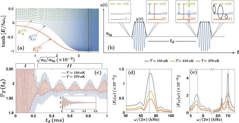
Figure 1: (a) Energy spectrum of three harmonically trapped ⁸⁵Rb particles with $\omega_{r}/(2\pi)=350\,\rm{Hz}$. Efimov trimer (T), atom-dimer (AD) and trap (A) states are depicted. Initially the scattering length is set at $a_{bg}=819\,a_{0}$ (dashed vertical line), then modulated with amplitude $a_{m}$ (gray region). Note $a_{0}$ is the Bohr radius. (b) A schematic illustration of the Ramsey-type interferometer: A first pulse with envelope $\chi(t)$ associates atom-dimers and Efimov states out of trap states (first and second sub-graphs in (b)), the system then evolves freely during the dark time $t_{d}$ (third sub-graph in (b)), while a second pulse further admixes the states together with their dynamical phases that were accumulated during $t_{d}$ (fourth sub-graph in (b)). (c) The ratio of thermally averaged (RTA) probabilities, $\mathbb{P}_{T}(t_{d})$ at $a_{bg}=819\,a_{0}$ and distinct temperatures (see legend). Inset: A zoom out plot of RTA at early $t_{d}$. (d) [(e)] Frequency spectra referring to region I [II] of the RTA quantifying its single [multifrequency] behavior at different values of temperature $\mathcal{T}$. The vertical dotted lines correspond to the three-level model (TLM) predictions for $E^{(2)}_{T}$, $E^{(1)}_{AD}$ and a trap state (see text).

Such an approach is developed here to investigate the three-body dynamics of a thermal gas. We consider ⁸⁵Rb atoms since the lifetimes of the ensuing trimers and dimers are known experimentally Klauss et al. (2017) in contrast to ⁷Li Yudkin et al. (2019). Our study establishes that, by implementing double magnetic field pulses, the intrinsic properties of Efimov trimers are readily probed regardless of the sign or magnitude of the scattering length; at which these states occur. Rich interferometric spectra exhibit both low- and high-frequencies independent of the gas temperature. The low-frequency components originate from the coherent superposition of the trimer with the dimer state, consistent with the observations in Ref. Yudkin et al. (2019). The additional high-frequencies arise from the coherent population of the trimer or dimer states with the ones lying at the “at break-up” threshold. The characteristic damping time of the field generated interference fringes is shown to be twice the lifetime of the Efimov trimers, providing an explanation for the unusually long decay times observed in Ref. Yudkin et al. (2019).

This work begins by introducing the time-dependent framework for the three-body system in Sec. II, providing also details on the employed techniques. Subsequently, in Sec. III, the association mechanisms of the dynamical scheme are examined. The role of the lifetime of the Efimov states is studied in Sec. IV for both repulsive and attractive background interactions. Sec. V summarizes our major findings and future perspectives are discussed. Appendix A outlines the steps to numerically solve the three-body time-dependent Schrödinger equation in hyperspherical coordinates, while the explicit form of the interaction potential matrix elements using field-free eigenstates is given in Appendix B. Further insights into the three-level model via first-order time-dependent perturbation theory are provided in Appendix C.

II Time-dependent three-body system and interferometry protocol

Our paradigm system consists of three ⁸⁵Rb atoms of mass $m$ confined in a spherically symmetric harmonic trap with radial frequency $\omega_{r}$. Following the prescription of Refs. Góral et al. (2004); Sykes et al. (2014); Corson and Bohn (2015); Borca et al. (2003); D’Incao et al. (2018); von Stecher and Greene (2007), we set $\omega_{r}=2\pi\times 350\rm{Hz}$ yielding a single atom trap length $a_{r}=\sqrt{\hbar/(m\omega_{r})}$, that compares to the interparticle spacing ($\sim\braket{n}^{-1/3}$) used in Ref. Klauss et al. (2017) for a local peak density $n_{0}=5\cdot 10^{12}\,\rm{cm}^{-3}$. The dynamics and the universal characteristics of the three-body system are addressed by employing contact interactions with a time-dependent $s$-wave scattering length, i.e. $a(t)$. The three-body Hamiltonian reads:

$$\mathcal{H}(t)=\sum_{i=1}^{3}\left(\frac{-\hbar^{2}\nabla_{i}^{2}}{2m}+\frac{m\omega_{r}^{2}}{2}\bm{r}_{i}^{2}\right)+\sum_{i<j}\frac{4\pi\hbar^{2}a(t)}{m}\delta(\bm{r}_{ij})\hat{O}_{ij},$$ (1)

where $\bm{r_{i}}$ denotes the position of the $i$-th atom, and $\hat{O}_{ij}=\partial_{r_{ij}}(r_{ij}\cdot)$ is the Fermi-Huang regularization operator with ${r}_{ij}=|{\bm{r}}_{i}-{\bm{r}}_{j}|$. Fig. 1(b) depicts the dynamical profile of $a(t)$ determined by the double pulse magnetic field sequence used in Ref. Yudkin et al. (2019), namely

$$a(t)=a_{bg}+a_{m}\cos{(\Omega t)}\Big{[}\chi(t)+\chi(t-t_{d}-2t_{0}-\tau)\Big{]},$$ (2)

$$\rm{with}~{}~{}\chi(t)=\begin{cases}\sin^{2}\left(\frac{\pi t}{2t_{0}}\right),&0\leq t<t_{0}\\ 1,&t_{0}\leq t<t_{0}+\tau\\ \sin^{2}\left(\frac{\pi(t-\tau)}{2t_{0}}\right),&t_{0}+\tau\leq t\leq 2t_{0}+\tau\\ 0,&\rm{otherwise}\end{cases}.$$ (3)

Here, $a_{bg}$ indicates the background scattering length of the time-independent system, and $a_{m}$ is the pulse’s amplitude yielding $\sim 20\%$ change to $a_{bg}$. $\Omega$ is the driving frequency and $\chi(t)$ denotes the envelope of the pulse where $t_{0}$ and $\tau$ are the ramp on/off times and length of the pulse envelope, respectively. The time between the two pulses is represented by $t_{d}$, i.e. dark time, where the system freely evolves.

Owing to Eq. 2, it suffices to simulate the corresponding time-dependent Schrödinger equation in the center-of-mass of the three-body system. Namely, only the relative Hamiltonian depends explicitly on time, i.e. $\mathcal{H}(t)=\mathcal{H}_{cm}+\mathcal{H}_{rel}(t)$. Regarding the center-of-mass Hamiltonian $\mathcal{H}_{cm}$ we assume from here on that the three-atom setting always resides in its ground state, $\ket{0}_{cm}$. Subsequently, the $\mathcal{H}_{rel}(t)$ is further decomposed into two terms: (i) a field-free Hamiltonian that describes three atoms in a spherical trap interacting with $a_{bg}$ scattering length and (ii) an explicit time-dependent interaction term [for more details see Section A.1]. The spectrum of the relative field-free Hamiltonian is obtained via the adiabatic hyperspherical approach Greene et al. (2017); Naidon and Endo (2017); D’Incao (2018); Nielsen et al. (2001); Rittenhouse et al. (2010). In this method all the relative degrees of freedom are expressed by a hyperradius $R$, that describes the overall system size, and a set of five hyperangles $\bm{\varpi}$, that address the relative particle positions. Subsequently, the field-free eigenstates $\ket{n}$ are expanded in a set of hyperangular basis functions, $\Phi_{\nu}(R;\bm{\varpi})$, treating the hyperradius as an adiabatic parameter Greene et al. (2017); Nielsen et al. (2001),

$$\braket{R,\bm{\varpi}}{n}=R^{-5/2}\sum_{\nu}F^{(n)}_{\nu}(R)\Phi_{\nu}(R;\bm{\varpi}),$$ (4)

where the expansion coefficients $F^{(n)}_{\nu}(R)$ are the so-called hyperradial channel functions.

Within the adiabatic hyperspherical approach, the determination of the eigenstates $\ket{n}$ along with their corresponding eigenenergies is performed in two steps. The hyperangular wavefunctions are obtained first, treating $R$ as an adiabatic parameter. Subsequently, the hyperradial channel functions and $E^{(n)}$ are calculated from the resulting equations that include all the relevant nonadiabatic coupling terms. A more elaborate discussion on the adiabatic hyperspherical approach is provided in Section A.2.

The stationary eigenenergies $E^{(n)}$ versus the scattering length $a_{bg}$ are shown in Fig. 1(a). Their corresponding eigenstates, $\ket{n}$, fall into three classes: Efimov trimers ($T$), atom-dimers ($AD$) and trap ($A$) states [red, blue and green lines in Fig. 1 (a)]. Furthermore, the adiabatic hyperspherical approach allows to express the time-dependent wave function of Eq. 1 in terms of the field-free eigenstates, i.e. $\ket{\Psi^{(\alpha)}_{3b}(t)}=\sum_{n}c^{(\alpha)}_{n}(t)\ket{n}\ket{0}_{cm}$ with $c^{(\alpha)}_{n}(t)$ being the probability amplitude of the $n$-th stationary state. The initial boundary condition is $c^{(\alpha)}_{n}(0)=\delta_{n\alpha}$ where the index $\alpha$ enumerates solely trap states, i.e. $\alpha\in A$. Plugging this expansion into the time-dependent Schrödinger equation (TDSE) under the Hamiltonian of Eq. (1) leads to a matrix differential equation for the time-dependent expansion coefficients,

$$i\hbar\frac{d\bm{c}^{(\alpha)}(t)}{dt}=\bm{\mathcal{H}}_{rel}(t)\cdot\bm{c}^{(\alpha)}(t).$$ (5)

Here, $\bm{\mathcal{H}}_{rel}(t)$ represents the relative Hamiltonian matrix expressed in the field-free basis. Given the decomposition of $\mathcal{H}_{rel}(t)$ into a field-free Hamiltonian and an explicit time-dependent interaction term, it is convenient to employ the second-order split-operator method Burstein and Mirin (1970); Tarana and Greene (2012) for solving Eq. 5 [for additional information refer also to Section A.3].

According to Fig. 1(b), initially the three particles interact with $a(t=0)=a_{bg}=819~{}a_{0}$ [see dashed vertical line in Fig. 1(a)] residing in a specific trap state. Similar to Ref. Yudkin et al. (2019), at $a_{bg}$ the system supports two Efimov trimer states, with the second (excited) one at energy $E_{T}^{(2)}$ lying close to the first atom-dimer energy in the trap, $E_{AD}^{(1)}$, which represents the atom-dimer threshold. At $t\neq 0$ the first pulse turns on with an envelope $\chi(t)$ of amplitude $a_{m}$ [gray region in Fig. 1 (a)], where $a(t)$ modulates with angular frequency $\Omega$ Giannakeas et al. (2019); Yudkin et al. (2019). The latter is equal to the energy difference between the first trap and atom-dimer states, i.e. $\Omega/2\pi=(E^{(1)}_{A}-E_{AD}^{(1)})/h=63.8~{}\rm{kHz}$, as in the experiment of Ref. Yudkin et al. (2019). Furthermore, the pulse’s full-width-at-half-maximum is $27\,{\rm\mu s}$ providing an energy bandwidth of $6.5~{}\rm{kHz}$ matching the energy difference between the second trimer and first atom-dimer states, $|E_{T}^{(2)}-E_{AD}^{(1)}|/h$. This implies that the first excited trimer $E_{T}^{(2)}$ and atom-dimer $E_{AD}^{(1)}$ states are coherently populated since the pulse cannot energetically resolve them. After the first pulse, the system occupies several $\ket{n}$ eigenstates which freely evolve during the dark time $t_{d}$, each accumulating a dynamic phase [see Fig. 1(b)]. At $t=t_{d}$, a second pulse, identical to the first one, is applied, admixing different stationary eigenstates and their corresponding dynamical phases. By the end of the second pulse, we extract the probability to occupy the Efimov trimer state as a function $t_{d}$.

In a typical experiment, the three-body dynamics takes place in a thermal gas at temperature $\mathcal{T}$ Yudkin et al. (2019, 2020). Hence, after the double pulse sequence the probability density to occupy the Efimov trimer needs to be thermally averaged over a Maxwell-Boltzmann ensemble of initial trap states. For our purposes, we introduce a ratio of thermally averaged (RTA) probabilities, $\mathbb{P}_{T}(t_{d})$, to populate Efimov trimer states after two pulses (numerator) versus one pulse (denominator),

$$\mathbb{P}_{T}(t_{d})=\frac{\sum_{\alpha\in A}\sum_{j\in\,T}e^{-\frac{E_{A}^{(\alpha)}}{k_{B}\mathcal{T}}}\left|c^{(\alpha)}_{j}(2\tilde{\tau}+t_{d})\right|^{2}}{\sum_{\alpha\in A}\sum_{j\in\,T}e^{-\frac{E_{A}^{(\alpha)}}{k_{B}\mathcal{T}}}\left|c^{(\alpha)}_{j}(\tilde{\tau})\right|^{2}},$$ (6a)

$$c^{(\alpha)}_{j}(2\tilde{\tau}+t_{d})=\sum_{n}U_{jn}(2\tilde{\tau}+t_{d},\tilde{\tau}+t_{d})e^{-iE^{(n)}t_{d}/\hbar}U_{n\alpha}(\tilde{\tau},0),$$ (6b)

where $k_{B}$ is the Boltzmann constant, $\tilde{\tau}=2t_{0}+\tau$ is the pulse duration, and $U_{ij}(\cdot,\cdot)$ represents the three-body evolution operator during a single pulse, expressed in the field-free basis.

III Dynamical superposition of Efimov trimers

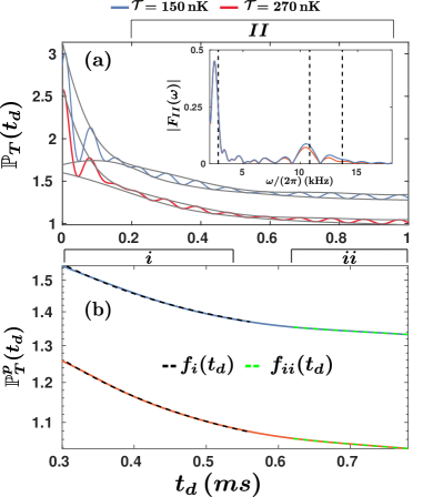
Figure 2: (a) $\mathbb{P}_{T}(t_{d})$ for different temperatures (see legend), taking into account the decay width, $\Gamma^{(2)}/h=748\,\rm{Hz}$ of the first excited Efimov state at $a_{bg}=2030\,a_{0}$. The gray solid lines outline the upper and lower peak envelopes. The inset presents the frequency spectrum pertaining to region II, $\left|F_{II}(\omega)\right|$. (b) The mean peak-to-peak envelope, $\mathbb{P}^{p}_{T}(t_{d})$ is fitted with the exponentials $f_{i/ii}(t_{d})=g_{i/ii}e^{-\Gamma_{i/ii}(t_{d}-t^{0}_{i/ii})/\hbar}+w_{i/ii}$ at dark time intervals $i$ and $ii$ (black and green dashed lines) with $g_{i/ii}$, $w_{i/ii}$ representing fitting constants. The characteristic decay time of the oscillations at long $t_{d}$ is twice as long as the intrinsic Efimov lifetime $\hbar/\Gamma^{(2)}$.

Fig. 1(c) depicts $\mathbb{P}_{T}(t_{d})$ for two characteristic temperatures $\mathcal{T}$, where oscillatory fringes are observed that persist after thermal averaging. Namely, $\mathbb{P}_{T}(t_{d})$ exhibits fast oscillations throughout regions I and II, and additional slow ones only in region II. The contributing frequencies are identified in the Fourier spectra of RTA demonstrated in panels (d) and (e) for regions I and II, respectively. In region I, independently of the temperature, a single frequency dominates in $\mathbb{P}_{T}(t_{d})$ at $\omega/(2\pi)=71.8\,\rm{kHz}$ [Fig. 1 (d)] corresponding to the energy difference $|E_{A}^{(1)}-E_{T}^{(2)}|/h$. For longer dark times (region II), three distinct frequencies occur, Fig. 1(e), with the high ones, i.e. $\omega/(2\pi)=63.7$ and $69.9\,\rm{kHz}$, referring to the superposition of the first trap state with the first atom-dimer and excited Efimov states, respectively. The low-frequency peak at $\omega/(2\pi)=6.5\,\rm{kHz}$ originates from interfering amplitudes between the first atom-dimer and first excited Efimov state pathways. Note that region II ($\sim 1.2\,\rm{kHz}$) shows better frequency resolution than region I ($\sim 10\,\rm{kHz}$), which results in small deviations between the highest frequencies in both regions. Due to the finite resolution, a small mismatch also occurs between the difference $69.9-63.7\,\rm{kHz}$ and the low frequency peak in region II. Similar low-frequency and temperature independent oscillatory fringes were also experimentally observed for ⁷Li atoms Yudkin et al. (2019, 2020). However, the present analysis reveals that high-frequency interferences are also imprinted in the RTA probability, where the early dark time fringes can be experimentally utilized to measure the Efimov binding energy at a given $a_{bg}$.

The fact that $\mathbb{P}_{T}(t_{d})$ features three main frequencies, irrespectively of $\mathcal{T}$, is traced back to the incoherent sum of the trimer probability [see Eq. 6a]. Namely, all contributions involving higher-lying trap states peter out, except for three arising from the ground trap state $E_{A}^{(1)}$, the first atom-dimer $E_{AD}^{(1)}$ and the first excited Efimov state $E_{T}^{(2)}$. This particular set of eigenstates survives upon the thermal average due to the specifics of the pulse and its envelope. Recall that the driving frequency is in resonance between the $E_{A}^{(1)}$ and $E_{AD}^{(1)}$ stationary eigenstates, whereas the duration of the pulse is short in order to coherently populate only the first atom-dimer and first excited Efimov states.

Focusing on this aspect, a three-level model (TLM) Hamiltonian containing $E^{(2)}_{T}$, $E^{(1)}_{AD}$ and a single trap state is constructed Lambropoulos and Petrosyan (2006). The three-level system is initialized in the single trap state and we apply square pulses of the scattering length [Eqs. (2) (3)] to trigger the dynamics of the three-body setup. Within this picture, the probability amplitude to occupy the first excited Efimov state at the end of the second pulse is obtained by employing first-order time-dependent perturbation theory [for additional details see also Appendix C]. Moreover, approximations for the energy levels of the trap states and the matrix elements to occupy the trimer state lead to analytical expressions for $\mathbb{P}_{T}(t_{d})$ [see also Appendix B and C]. It is shown that the latter is decomposed into three oscillatory terms. The TLM predictions for the frequencies, illustrated as vertical dotted lines in Figs. 1 (d), (e), are found to be in excellent agreement with the full numerical calculations.

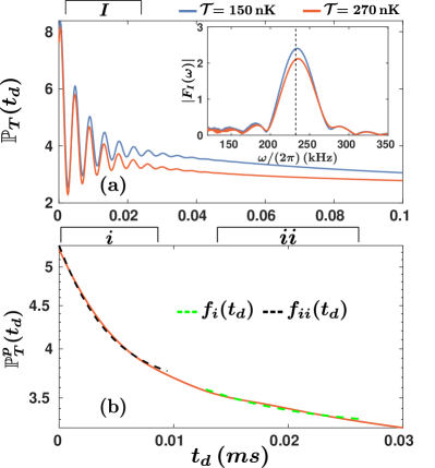
Figure 3: (a) $\mathbb{P}_{T}(t_{d})$ at $a_{bg}=-2030\,a_{0}$ and various temperatures (see legend). The driving frequency is resonant with the transition between the ground Efimov and the first trap state, and the decay width of the former $\Gamma^{(1)}/h=41\,\rm{kHz}$. The inset presents the frequency spectrum of region I, $\left|F_{I}(\omega)\right|$. (b) The mean peak-to-peak envelope, $\mathbb{P}^{p}_{T}(t_{d})$ at $\mathcal{T}=270\,\rm{nK}$ is fitted with $f_{i/ii}(t_{d})=g_{i/ii}e^{-\Gamma_{i/ii}(t_{d}-t^{0}_{i/ii})/\hbar}+w_{i/ii}$ at the dark time intervals $i$ and $ii$. Even at attractive interactions the energy and lifetime of Efimov states can be simultaneously assessed.

IV Impact of the lifetime of the trimer

In Fig. 1(c)-(e), our analysis neglects the decay of the Efimov trimers and dimer states. However, in thermal gases three-body recombination or relaxation processes are present resulting in finite lifetimes of the trimers and dimers. In the following, we choose $a_{bg}=2030\,a_{0}$ that is significantly larger than the van der Waals length scale $l_{VdW}=82.5\,a_{0}$ for ⁸⁵Rb, yielding negligible finite range effects Chin et al. (2010). Therefore, in this universal regime, the zero-range theory predicts that the lifetime of the first excited Efimov state is $\hbar/\Gamma^{(2)}=212\,\mu s$ ($\Gamma^{(2)}$ denotes the decay width) Werner and Castin (2006); Petrov et al. (2004); Nielsen et al. (2002); Klauss et al. (2017). Also, since the decay of dimers lie within the range 2-9 $ms$, for local peak density $n_{0}=5\cdot 10^{12}\,\rm{cm}^{-3}$ Braaten and Hammer (2004); Claussen et al. (2003); Köhler et al. (2005), they can be safely neglected within the considered range, $t_{d}\leq 1~{}\rm{ms}$, rendering the lifetime of Efimov trimers the most relevant decay mechanism. Furthermore, the pulse frequency is $\Omega/2\pi=10.8~{}\rm{kHz}$ over a time span $2t_{0}+\tau=134.7\,\mu s$ ensuring that the Efimov trimers do not decay during the pulse. Under these considerations, it suffices after the first pulse to multiply the amplitude of the $E_{T}^{(2)}$ state with the factor $e^{-\Gamma^{(2)}t_{d}/(2\hbar)}$, as was employed in Refs. Colussi et al. (2018b, 2019).

The interference fringes of the RTA probability including the effect of the decay at 150 and 270 nK are provided in Fig. 2(a). Owing to the large $a_{bg}$, the frequencies are in the range of tenths of kHz adequately agreeing with the TLM calculations [see dashed lines in the inset Fig. 2 (a)]. Isolating the impact of the Efimov states decay on the RTA probability, Fig. 2 (b) shows the mean peak-to-peak envelopes of $\mathbb{P}_{T}(t_{d})$, i.e. $\mathbb{P}^{p}_{T}(t_{d})$. Fitting $\mathbb{P}^{p}_{T}(t_{d})$ with $f_{i/ii}(t_{d})=g_{i/ii}e^{-\Gamma_{i/ii}(t_{d}-t^{0}_{i/ii})/\hbar}+w_{i/ii}$ at the dark time intervals $i$ and $ii$ [see dashed lines in Fig. 2 (b)] reveals two distinct decay widths independent of the temperature. Namely, $\Gamma_{i}/h=749.925(1.47)\,\rm{Hz}$ close to $\Gamma^{(2)}/h$, while at later $t_{d}$, $\Gamma_{ii}/h=375.03(1.63)~{}\rm{Hz}$, approximately $\Gamma^{(2)}/(2h)$. This means that at early dark times $\mathbb{P}_{T}(t_{d})$ falls off according to the intrinsic lifetime of the $E^{(2)}_{T}$ Efimov trimer. In region II, where the interference between the first atom-dimer and the first excited trimer is pronounced, the decay of the RTA probability is nearly twice the lifetime of the $E^{(2)}_{T}$ state. This effect can in principle explain the unusually long decay times observed in the experiment Yudkin et al. (2019).

Including the trimer’s lifetime in the TLM allows to gain insights on the decay of the RTA probability, where $\mathbb{P}_{T}(t_{d})$ becomes proportional to

$$\mathbb{P}_{T}(t_{d})\propto[\mathbb{B}_{T,A}(t_{d})+\mathbb{B}_{T,AD}(t_{d})]e^{-\frac{\Gamma^{(2)}t_{d}}{2\hbar}}+\mathbb{B}_{AD,A}(t_{d})$$

$$+e^{-\frac{\Gamma^{(2)}t_{d}}{\hbar}}.$$ (7)

The terms $\mathbb{B}_{i,j}(t_{d})=A_{i,j}(t_{d})\sin\left[(E^{(\sigma)}_{i}-E^{(1)}_{j})t_{d}/\hbar\right]$ with $\sigma=1+\delta_{i,T}$ originate from the superposition of states $i$, $j$, and $A_{i,j}(t_{d})$ refer to their amplitudes (see details in Appendix C). The first three terms correspond to the three dominant frequencies shown as dashed lines in the inset of Fig. 2 (a). The mixed contributions that involve $E^{(2)}_{T}$ with another state, contain only the factor $e^{-\Gamma^{(2)}t_{d}/(2\hbar)}$. Therefore, within region II where the coherent admixture between the $E_{AD}^{(1)}$ and $E_{T}^{(2)}$ states is manifested, the decay time of $\mathbb{P}_{T}(t_{d})$ is virtually twice as long as the intrinsic Efimov lifetime. The last non-oscillatory term in Eq. 7 involves only the Efimov state and thus decays according to $e^{-\Gamma^{(2)}t_{d}/\hbar}$. The above expression holds in general for any atomic species and $a_{bg}>0$, provided that both the first excited Efimov and first atom-dimer are coherently populated.

As a generalization, the RTA probability is demonstrated in Fig. 3 at negative scattering lengths, e.g. $a_{bg}=-2030\,a_{0}$, where the atom-dimer pathways are intrinsically absent since no universal dimer exists. The pulse frequency $\Omega/2\pi=|E_{T}^{(1)}-E_{A}^{(1)}|/h=232.2~{}\rm{kHz}$ and its duration is $2t_{0}+\tau=3.7\,\mu s$. Note that here the pulse resonantly couples the first trap and the Efimov ground state, whereas the pulse’s length is shorter than the ground Efimov state lifetime $\hbar/\Gamma^{(1)}$=3.9  $\mu s$ Braaten and Hammer (2006). As expected, the $\mathbb{P}_{T}(t_{d})$ in Fig. 3(a) oscillates with a single frequency, i.e. $\omega/(2\pi)=\left|E^{(1)}_{T}-E^{(1)}_{A}\right|/h=233.5\,\rm{kHz}$, only in region I and vanishes fast due to the large $\Gamma^{(1)}$ decay width. Moreover, Fig. 3(b) showcases the mean peak-to-peak amplitude $\mathbb{P}^{p}_{T}(t_{d})$ and their fittings at the dark time intervals $i$ and $ii$ [see dashed lines in Fig. 3 (b)]. Similar to Fig. 2 (b), we extract two decay widths with their values being $\Gamma_{i}/h=41.35(5.35)\,\rm{kHz}$ and $\Gamma_{ii}/h=17.56(7.02)\,\rm{kHz}$ at $\mathcal{T}=270\,\rm{nK}$, which within error bars are close to $\Gamma^{(1)}/h$ and $\Gamma^{(1)}/(2h)$, respectively. These findings are in accordance to the description of Eq. 7, omitting terms associated with atom-dimer transitions.

V Conclusions and outlook

In summary, the present theory demonstrates that the double magnetic field interferometer has broad applicability. Namely, it permits the simultaneous extraction of the binding energy and the lifetime of Efimov states regardless the sign/magnitude of the scattering length and the temperature of the gas. This is feasible due to the generated superpositions of the trimer with the first atom-dimer and trap state at repulsive interactions, or only with the first trap eigenstate at attractive interactions. These superpositions are manifested as interference (Ramsey) fringes in the probability to occupy trimers, observed over a wide range of temperatures. Corroborating our results, a three-level model is constructed, taking into account only the contributions stemming from the Efimov trimer, the first atom-dimer and trap state.

Going beyond previous studies, our analysis demonstrates that the Ramsey fringes possess long damping times equal to twice the intrinsic lifetime of Efimov trimers. This behavior is illustrated at long dark times between the pulses, attributed to the superposition of the trimer with the first atom-dimer state. This relation in particular provides also an upper bound to the lifetime of ⁷Li Efimov trimers which has remained unknown to date. Furthermore, our work predicts that there are additional interference terms surviving the thermal average at short dark times. Namely, in this regime the system exhibits interference fringes with frequencies that coincide with the binding energy of the Efimov states, whereas the decay of these oscillations is dictated by the lifetime of the trimers. This demonstrates that it is possible to extract the binding energy of the trimer at this early dark time regime, irrespective of the interaction strength. This extends the current experimental practice, exploring the long dark time region Yudkin et al. (2023, 2019).

Owing to the sensitivity of the Ramsey-type dynamical protocol, the corresponding interferometric signals could be further employed for probing Efimov states especially at attractive interactions. At this regime, trimers merge with the three-atom continuum at a scattering length related only to the van der Waals length, the so-called van der Waals universality Etrych et al. (2023); Xie et al. (2020); Berninger et al. (2011); Johansen et al. (2017); Naidon et al. (2014); Wang et al. (2012). The interferometry scheme can thus be utilized at this regime, providing stringent tests on the universality. Furthermore, recent experiments explore the modifications of three-body recombination processes in mixtures of a bosonic thermal gas with a degenerate fermion gas Chen et al. (2022). Hence, creation of dynamically coherent superpositions between few-body states can reveal the influence of a dense many-body environment on them.

Appendix A The three-body time-dependent Schrödinger equation in hyperspherical coordinates

The time-dependent three-body Hamiltonian is decomposed in the center-of-mass frame and further expressed in hyperspherical coordinates. An expansion in the field-free eigenstates is subsequently utilized to cast the TDSE in matrix form, tackled with the split operator method.

A.1 Center-of-mass decomposition

According to Eq. (1) in the main text, the three-body Hamiltonian in the laboratory frame reads

$$\mathcal{H}(t)=\sum_{i=1}^{3}\left(\frac{-\hbar^{2}\nabla_{i}^{2}}{2m}+\frac{m\omega_{r}^{2}}{2}\bm{r}_{i}^{2}\right)+\sum_{i<j}\frac{4\pi\hbar^{2}a(t)}{m}\delta(\bm{r}_{ij})\hat{O}_{ij}.$$ (8)

In order to eliminate the three degrees of freedom associated to the center-of-mass Hamiltonian we perform a transformation from the laboratory to the center-of-mass frame. The Hamiltonian splits into a time-independent center-of-mass part and another one describing the relative degrees of freedom, i.e. $\mathcal{H}(t)=\mathcal{H}_{cm}+\mathcal{H}_{rel}(t)$. Evidently, $\mathcal{H}_{rel}(t)$ encapsulates the relevant three-body dynamics, which in hyperspherical coordinates, Rittenhouse et al. (2010); Greene et al. (2017); Bougas et al. (2021) takes the following expression

$$\mathcal{H}_{rel}(t)=-\frac{\hbar^{2}}{2\mu}\frac{1}{R^{5/2}}\frac{\partial^{2}}{\partial R^{2}}\left(R^{5/2}\cdot\right)+\frac{15\hbar^{2}}{8\mu R^{2}}+\frac{\hbar^{2}\bm{\Lambda}^{2}}{2\mu R^{2}}$$

$$+\frac{1}{2}\mu\omega^{2}_{r}R^{2}+V_{bg}(R;\bm{\varpi})+V(R;\bm{\varpi})f(t).$$ (9)

In this coordinate system, $R$ describes the overall system size, and the five hyperangles collectively indicated by $\bm{\varpi}$ address the relative particle positions. $V_{bg}(R;\bm{\varpi})$ and $V(R;\bm{\varpi})$ are the contact interaction potentials associated to the background ($a_{bg}$) and amplitude scattering length ($a_{m}$) respectively, expressed in hyperspherical coordinates. Moreover, we have isolated the time-dependence in the function $f(t)=[a(t)-a_{bg}]/a_{m}$. $\bm{\Lambda}^{2}$ is the grand angular momentum operator describing the total angular momentum of the three atoms Avery (1989), and $\mu$ is the three-body reduced mass.

According to Eq. 9, $\mathcal{H}_{rel}(t)$ splits into a field-free Hamiltonian that describes three particles interacting with $a_{bg}$ scattering length and a time-dependent part which contains the pulse field, i.e. $\mathcal{H}_{rel}(t)=\mathcal{H}_{bg}+V(R;\bm{\varpi})f(t)$. This particular structure of $\mathcal{H}_{rel}(t)$ suggests that the time-dependent three-body wave function pertaining to the Hamiltonian Eq. 8 can be conveniently expanded on the field-free basis set, $\ket{n}$, a basis such that $\mathcal{H}_{bg}$ is a diagonal matrix.

A.2 Eigenstates of the background Hamiltonian

Therefore, in order to obtain the eigenstates $\{\ket{n}\}$ of $\mathcal{H}_{bg}$, we employ the adiabatic hyperspherical representation Greene et al. (2017); Nielsen et al. (2001), where the hyperradius $R$ is treated as an adiabatic parameter. For completeness reasons, a brief description on the calculation of $\ket{n}$ in this formalism is provided below. Namely, $\mathcal{H}_{bg}$ is recasted as follows:

$$\mathcal{H}_{bg}=-\frac{\hbar^{2}}{2\mu}\frac{1}{R^{5/2}}\frac{\partial^{2}}{\partial R^{2}}\left(R^{5/2}\cdot\right)$$

$$+\underbrace{\frac{15\hbar^{2}}{8\mu R^{2}}+\frac{\hbar^{2}\bm{\Lambda}^{2}}{2\mu R^{2}}+\frac{1}{2}\mu\omega^{2}_{r}R^{2}+V_{bg}(R;\bm{\varpi})}_{\mathcal{H}_{ad}(R;\bm{\varpi)}},$$ (10)

where $\mathcal{H}_{ad}(R;\bm{\varpi})$ refers to the adiabatic hyperangular Hamiltonian which parametrically depends on the hyperradius $R$. In addition, the eigenstates $\ket{n}$ are expressed by the ansatz

$$\braket{R,\bm{\varpi}}{n}=R^{-5/2}\sum_{\nu}F_{\nu}^{(n)}(R)\Phi_{\nu}(R;\bm{\varpi}),$$ (11)

where $F^{(n)}_{\nu}(R)$ [$\Phi_{\nu}(R;\bm{\varpi})$] denotes the hyperradial [hyperangular] component of $\ket{n}$. More specifically, $\Phi_{\nu}(R;\bm{\varpi})$ are obtained by diagonalizing $\mathcal{H}_{ad}(R;\bm{\varpi})$ at fixed hyperradius $R$ Rittenhouse et al. (2010); Bougas et al. (2021) according to the expression

$$\mathcal{H}_{ad}(R;\bm{\varpi})\Phi_{\nu}(R;\bm{\varpi})=U_{\nu}(R)\Phi_{\nu}(R;\bm{\varpi}),$$ (12)

where $U_{\nu}(R)$ represents the $\nu$-th hyperspherical potential curve that depends only on $R$. The hyperradial functions $F^{(n)}_{\nu}(R)$ are determined by acting with $\mathcal{H}_{bg}$ on $\ket{n}$ and integrating over all the hyperangles $\bm{\varpi}$. This yields a system of coupled hyperradial equations that include the non-adiabatic couplings Rittenhouse et al. (2010); Greene et al. (2017). By diagonalizing the resulting matrix equations we obtain the eigenenergies $E^{(n)}$ and hyperradial wave functions $F^{(n)}_{\nu}(R)$ Rittenhouse et al. (2010); Greene et al. (2017).

A.3 Solution of the TDSE

Expanding the time-dependent three-body wave function in terms of $\ket{n}$ yields the following relation:

$$\ket{\Psi^{(\alpha)}_{3b}(t)}=\sum_{n}c^{(\alpha)}_{n}(t)\ket{n}\ket{0}_{cm},$$ (13)

where the time-dependent coefficients initially satisfy $c^{(\alpha)}_{n}(t=0)=\delta_{n\alpha}$, and the $\alpha$ index refers to an initial trap state. $\ket{0}_{cm}$ is the center-of-mass ground state.

Plugging Eq. 13 into the TDSE under the Hamiltonian of Eq. 8 leads to a matrix differential equation for the time-dependent expansion coefficients,

$$i\hbar\frac{d\bm{c}^{(\alpha)}(t)}{dt}=(\bm{\mathcal{H}_{bg}}+f(t)\bm{V})\cdot\bm{c}^{(\alpha)}(t).$$ (14)

Eq. 14 is solved numerically by utilizing the second-order split-operator method Burstein and Mirin (1970). Namely, the propagator of the $\bm{c}^{(\alpha)}(t)$ vectors within the time interval ($t$, $t+dt$) reads

$$\bm{c}^{(\alpha)}(t+dt)=e^{-i\bm{\mathcal{H}_{bg}}dt/(2\hbar)}e^{-i\bm{V}/\hbar\int_{t}^{t+dt}dt^{\prime}\,f(t^{\prime})}$$

$$\times e^{-i\bm{\mathcal{H}_{bg}}dt/(2\hbar)}\bm{c}^{(\alpha)}(t)+\mathcal{O}(dt^{3}).$$ (15)

Appendix B Matrix elements of the interaction potential with the field-free eigenstates

Having at hand the set of field-free eigenstates $\{\ket{n}\}$, obtained from the adiabatic hyperspherical formalism, the matrix elements of the interaction potential associated to $a_{m}$, $\bm{V}_{n^{\prime}n}$, can be evaluated as

$$\bm{V}_{n^{\prime}n}=\sum_{\nu,\nu^{\prime}}\int dR\>F^{(n^{\prime})*}_{\nu^{\prime}}(R)\mathcal{M}_{\nu^{\prime}\nu}(R)F^{(n)}_{\nu}(R),$$ (16)

$$\mathcal{M}_{\nu^{\prime}\nu}(R)=\braket{\Phi_{\nu^{\prime}}(R)}{V}{\Phi_{\nu}(R)}_{\bm{\varpi}},$$ (17)

where $\braket{\cdot}_{\bm{\varpi}}$ indicates that the integral is performed over the hyperangles.

Eq. (17) can be recasted in a simple form by exploiting the property $V(R;\bm{\varpi})=-(a_{m}/a_{bg})\frac{R}{3}\partial_{R}V_{bg}(R;\bm{\varpi})$ between the contact potentials and utilizing the Hellman-Feynman theorem Feynman (1939). Namely, for $\nu\neq\nu^{\prime}$ the relation $\mathcal{M}_{\nu^{\prime}\nu}(R)=-(a_{m}/a_{bg})R\braket{\Phi_{\nu^{\prime}}(R)}{\partial_{R}\Phi_{\nu}(R)}_{\bm{\varpi}}[U_{\nu^{\prime}}(R)-U_{\nu}(R)]$ holds. Similar expressions are derived for $\nu=\nu^{\prime}$ which can be regrouped as follows

$$\mathcal{M}_{\nu^{\prime}\nu}(R)=\frac{a_{m}}{a_{bg}}\frac{\hbar^{2}}{2\mu R}(-)^{1+\rm{sgn}(\nu-\nu^{\prime})}\sqrt{\partial_{R}s^{2}_{\nu}(R)\partial_{R}s^{2}_{\nu^{\prime}}(R)}.$$ (18)

Here, $s^{2}_{\nu}(R)$ are related to the potential curves, i.e. $2\mu R^{2}/\hbar^{2}U_{\nu}(R)=s^{2}_{\nu}(R)-1/4$, and $\rm{sgn}(\cdot)$ denotes the sign function.

Appendix C Three-level model and perturbation theory

To provide a simplified picture of the full dynamics of the few-body bound states we next construct an effective three-level model. Within this model, we consider only three field-free eigenstates, the first excited Efimov trimer (T), the first atom-dimer (AD) and an initial trap state $\alpha$.

At the end of the first pulse, the probability amplitude to occupy the $T$ state, $\bar{c}^{(\alpha)}_{T}$, within first-order time-dependent perturbation theory Sakurai (1967), reads

$$\bar{c}^{(\alpha)}_{T}(t_{0}+\tau)=\bm{V}_{T,\alpha}R_{T,\alpha}(t_{0}+\tau),$$ (19a)

$$R_{n,m}(t_{0}+\tau)=\frac{-e^{i(\omega_{n,m}+\Omega)(t_{0}+\tau)/2}\sin\left[(\omega_{n,m}+\Omega)\frac{t_{0}+\tau}{2}\right]}{\hbar(\omega_{n,m}+\Omega)}$$

$$-(\Omega\leftrightarrow-\Omega),$$ (19b)

where $\omega_{n,m}\equiv(E^{(n)}-E^{(m)})/\hbar$.

During the dark time $t_{d}$, the probability amplitude of the $n$-th state acquires the phase factor $e^{-iE^{(n)}t_{d}/\hbar}\bar{c}^{(\alpha)}_{n}(t_{0}+\tau)$. In particular, the amplitude of the first excited Efimov state is supplemented with the factor $e^{-\Gamma^{(2)}t_{d}/(2\hbar)}$, due to the width $\Gamma^{(2)}$ of the Efimov state, leading to the decay of the latter during $t_{d}$.

The second pulse mixes all states together, and the probability amplitude to occupy the $T$ state at the end of this pulse reads,

$$\bar{d}^{(\alpha)}_{T}(2t_{0}+2\tau+t_{d})=\sum_{j=T,AD}\Big{[}\bm{V}_{T,j}R_{T,j}(t_{0}+\tau)$$

$$\times\bar{c}^{(\alpha)}_{j}(t_{0}+\tau)e^{-iE^{(\sigma)}_{j}t_{d}/\hbar-\Gamma^{(2)}t_{d}/(2\hbar)\delta_{T,j}}\Big{]}$$

$$+\bm{V}_{T,\alpha}R_{T,\alpha}(t_{0}+\tau)\bar{c}^{(\alpha)}_{A}(t_{0}+\tau)e^{-iE^{(\alpha)}_{A}t_{d}/\hbar},$$ (20)

where $\sigma=1+\delta_{j,T}$.

To obtain the ratio of the thermally averaged probability $\mathbb{P}_{T}(t_{d})$, we weight the probabilities $\left|\bar{d}^{(\alpha)}_{T}(2t_{0}+2\tau+t_{d})\right|^{2}$ and $\left|\bar{c}^{(\alpha)}_{T}(t_{0}+\tau)\right|^{2}$ according to the Maxwell-Boltzman distribution for the trap states of energy $E_{A}^{(\alpha)}$ at temperature $\mathcal{T}$,

$$\mathbb{P}_{T}(t_{d})=\frac{\sum_{\alpha\in A}e^{-\frac{E_{A}^{(\alpha)}}{k_{B}\mathcal{T}}}\left|\bar{d}^{(\alpha)}_{T}(2t_{0}+2\tau+t_{d})\right|^{2}}{\sum_{\alpha\in A}e^{-\frac{E_{A}^{(\alpha)}}{k_{B}\mathcal{T}}}\left|\bar{c}^{(\alpha)}_{T}(t_{0}+\tau)\right|^{2}},$$ (21)

where $k_{B}$ is the Boltzmann constant.

In order to derive an analytical expression for Eq. 21 additional approximations are used. Namely, the expressions for $\bar{d}_{T}^{(\alpha)}(2t_{0}+2\tau+t_{d})$ and $\bar{c}^{(\alpha)}_{T}(t_{0}+\tau)$ can be further simplified by employing the rotating-wave approximation Sakurai (1967).

Furthermore, the energy of the $\alpha$-th trap state is roughly approximated by the non-interacting energy spectrum, $E_{A}^{(\alpha)}=E_{A}^{(1)}+2\alpha\hbar\omega_{r}$, where $E^{(1)}_{A}$ is the energy of the first trap state. In addition, we approximate the $\bm{V}_{T,\alpha}$ matrix elements with a quartic root of the energy of the $\alpha$-th trap state, a dependence corroborated by a fitting procedure. Under these considerations, Eq. (21) obtains the same form as Eq. (5) in the main text,

$$\mathbb{P}_{T}(t_{d})\propto[\mathbb{B}_{T,A}(t_{d})+\mathbb{B}_{T,AD}(t_{d})]e^{-\Gamma^{(2)}t_{d}/(2\hbar)}+\mathbb{B}_{AD,A}(t_{d})+e^{-\Gamma^{(2)}t_{d}/\hbar},$$ (22)

where the $\mathbb{B}$-terms are given by the expressions

$$\mathbb{B}_{T,A}(t_{d})=C_{1}\>\Im\Bigg{[}e^{-i\Delta\phi_{1}}\Phi\left(e^{f(k_{B}\mathcal{T},t_{d},\omega_{r})},-0.5,\frac{E^{(1)}_{A}}{2\hbar\omega_{r}}\right)\Bigg{]}$$ (23a)

$$\mathbb{B}_{T,AD}(t_{d})=\sum_{\pm}(-)^{\pm}C_{2}^{\pm}\sin\left[(E^{(2)}_{T}-E^{(1)}_{AD})t_{d}/\hbar\pm\Omega(t_{0}+\tau)/2\right]$$ (23b)

$$\mathbb{B}_{AD,A}(t_{d})=\sum_{\pm}C_{3}^{\pm}\,\Re\Bigg{[}e^{-i\Delta\phi_{2}\pm i\Omega(t_{0}+\tau)/2}\Phi\left(e^{f(k_{B}\mathcal{T},t_{d},\omega_{r})},-0.5,\frac{E^{(1)}_{A}}{2\hbar\omega_{r}}\right)\Bigg{]}$$ (23c)

$$f(k_{B}\mathcal{T},t_{d},\omega_{r})=-\frac{2\hbar\omega_{r}}{k_{B}\mathcal{T}}+2i\omega_{r}[t_{d}+1.5(t_{0}+\tau)].$$ (23d)

$\Phi(a,b,z)$ is the Hurwitz-Lersch zeta function Gradshteyn et al. (2015) and the phases $\Delta\phi_{1}$ and $\Delta\phi_{2}$ are defined as follows,

$$\Delta\phi_{1}\equiv\frac{(E^{(2)}_{T}-E^{(1)}_{A})t_{d}}{\hbar}-3E^{(1)}_{A}\frac{t_{0}+\tau}{2\hbar}$$ (24)

$$\Delta\phi_{2}\equiv\frac{(E^{(1)}_{AD}-E^{(1)}_{A})t_{d}}{\hbar}-3E^{(1)}_{A}\frac{t_{0}+\tau}{2\hbar}.$$ (25)

The explicit form of the prefactors $C_{1},C_{2}^{\pm},C_{3}^{\pm}$ is given by,

$$C_{1}=\frac{\hbar\Omega}{\bm{V}_{T,T}}\frac{\left[\Phi\left(e^{-2\hbar\omega_{r}/(k_{B}\mathcal{T})},-0.5,\frac{E^{(1)}_{A}}{2\hbar\omega_{r}}\right)\right]^{-1}}{\sin^{2}[\Omega(t_{0}+\tau)/2]},$$ (26)

$$C_{2}^{\pm}=\frac{\bm{V}_{T,AD}}{\bm{V}_{T,T}}\frac{\hbar\Omega}{\sin^{2}[\Omega(t_{0}+\tau)/2]}$$

$$\times\frac{\sin[(\omega_{T,AD}\pm\Omega)(t_{0}+\tau)/2]}{\hbar(\omega_{T,AD}\pm\Omega)},$$ (27)

$$C_{3}^{\pm}=(-)^{\pm}\frac{\bm{V}_{T,AD}}{\left|\bm{V}_{T,T}\right|^{2}}\frac{\sin[(\omega_{T,AD}\pm\Omega)(t_{0}+\tau)/2]}{2\hbar(\omega_{T,AD}\pm\Omega)}$$

$$\frac{\hbar^{2}\Omega^{2}}{\sin^{4}[\Omega(t_{0}+\tau)/2]}\times\left[\Phi\left(e^{-2\hbar\omega_{r}/(k_{B}\mathcal{T})},-0.5,\frac{E^{(1)}_{A}}{2\hbar\omega_{r}}\right)\right]^{-1},$$ (28)

Note that there are revivals of the oscillatory signals $\mathbb{B}_{T,A}(t_{d})$ and $\mathbb{B}_{AD,A}(t_{d})$ at later dark times $\frac{n\pi}{\omega_{r}}-1.5(t_{0}+\tau)$, which are attributed to the trap D’Incao et al. (2018).

References

- Efimov (1970) V. Efimov, “Energy levels arising from resonant two-body forces in a three-body system,” Phys. Lett. B 33, 563–564 (1970).
- Efimov (1973) V. Efimov, “Energy levels of three resonantly interacting particles,” Nucl. Phys. A 210, 157–188 (1973).
- Efimov (1971) V. N. Efimov, “Weakly bound states of three resonantly interacting particles.” Sov. J. Nucl. Phys. 12, 589 (1971).
- Greene et al. (2017) C. H. Greene, P. Giannakeas, and J. Pérez-Ríos, “Universal few-body physics and cluster formation,” Rev. Mod. Phys. 89, 035006 (2017).
- Nielsen et al. (2001) E. Nielsen, D. V. Fedorov, A. S. Jensen, and E. Garrido, “The three-body problem with short-range interactions,” Phys. Rep. 347, 373–459 (2001).
- Naidon and Endo (2017) P. Naidon and S. Endo, “Efimov physics: a review,” Rep. Prog. Phys. 80, 056001 (2017).
- D’Incao (2018) J. P. D’Incao, “Few-body physics in resonantly interacting ultracold quantum gases,” J. Phys. B: At. Mol. Opt. Phys. 51, 043001 (2018).
- Kraemer et al. (2006) T. Kraemer, M. Mark, P. Waldburger, J. G. Danzl, C. Chin, B. Engeser, A. D. Lange, K. Pilch, A. Jaakkola, H.-C. Nägerl, and R. Grimm, “Evidence for efimov quantum states in an ultracold gas of caesium atoms,” Nature 440, 315–318 (2006).
- Kunitski et al. (2015) M. Kunitski, S. Zeller, J. Voigtsberger, A. Kalinin, L. Ph. H. Schmidt, M. Schöffler, A. Czasch, W. Schöllkopf, R. E. Grisenti, T. Jahnke, D. Blume, and R. Dörner, “Observation of the efimov state of the helium trimer,” Science 348, 551–555 (2015).
- Endo et al. (2016) S. Endo, A. M. García-García, and P. Naidon, “Universal clusters as building blocks of stable quantum matter,” Phys. Rev. A 93, 053611 (2016).
- Kievsky et al. (2021) A. Kievsky, M. Gattobigio, L. Girlanda, and M. Viviani, “Efimov physics and connections to nuclear physics,” Annu. Rev. Nucl. Part. Sci. 71, 465–490 (2021).
- Nishida et al. (2013) Y. Nishida, Y. Kato, and C. D. Batista, “Efimov effect in quantum magnets,” Nature Phys. 9, 93–97 (2013).
- Gullans et al. (2017) M.J. Gullans, S. Diehl, S.T. Rittenhouse, B.P. Ruzic, J.P. D’Incao, P. Julienne, A.V. Gorshkov, and J.M. Taylor, “Efimov states of strongly interacting photons,” Phys. Rev. Lett. 119, 233601 (2017).
- Tran et al. (2021) B. Tran, M. Rautenberg, M. Gerken, E. Lippi, B. Zhu, J. Ulmanis, M. Drescher, M. Salmhofer, T. Enss, and M. Weidemüller, “Fermions meet two bosons—the heteronuclear efimov effect revisited,” Braz. J. Phys. 51, 316–322 (2021).
- Christianen et al. (2022) A. Christianen, J. I. Cirac, and R. Schmidt, “Bose polaron and the efimov effect: A gaussian-state approach,” Phys. Rev. A 105, 053302 (2022).
- Naidon (2018) P. Naidon, “Two impurities in a bose–einstein condensate: From yukawa to efimov attracted polarons,” J. Phys. Soc. Jpn. 87, 043002 (2018).
- Sun and Cui (2019) M. Sun and X. Cui, “Efimov physics in the presence of a fermi sea,” Phys. Rev. A 99, 060701 (2019).
- Musolino et al. (2022) S. Musolino, H. Kurkjian, M. Van Regemortel, M. Wouters, S. J. J. M. F. Kokkelmans, and V. E. Colussi, “Bose-einstein condensation of efimovian triples in the unitary bose gas,” Phys. Rev. Lett. 128, 020401 (2022).
- Colussi et al. (2018a) V. E. Colussi, S. Musolino, and S. J. J. M. F. Kokkelmans, “Dynamical formation of the unitary bose gas,” Phys. Rev. A 98, 051601 (2018a).
- Makotyn et al. (2014) P. Makotyn, C. E. Klauss, D. L. Goldberger, E. A. Cornell, and D. S. Jin, “Universal dynamics of a degenerate unitary bose gas,” Nature Phys. 10, 116–119 (2014).
- Eigen et al. (2018) C. Eigen, J. A. P. Glidden, R. Lopes, E. A. Cornell, R. P. Smith, and Z. Hadzibabic, “Universal prethermal dynamics of bose gases quenched to unitarity,” Nature 563, 221–224 (2018).
- Klauss et al. (2017) C. E. Klauss, X. Xie, C. Lopez-Abadia, J. P. D’Incao, Z. Hadzibabic, D. S. Jin, and E. A. Cornell, “Observation of efimov molecules created from a resonantly interacting bose gas,” Phys. Rev. Lett. 119, 143401 (2017).
- Fletcher et al. (2017) R. J. Fletcher, R. Lopes, J. Man, N. Navon, R. P. Smith, M. W. Zwierlein, and Z. Hadzibabic, “Two-and three-body contacts in the unitary bose gas,” Science 355, 377–380 (2017).
- Chen et al. (2022) X.-Y. Chen, M. Duda, A. Schindewolf, R. Bause, I. Bloch, and X.-Y. Luo, “Suppression of unitary three-body loss in a degenerate bose-fermi mixture,” Phys. Rev. Lett. 128, 153401 (2022).
- Donley et al. (2002) E. A. Donley, N. R. Claussen, S. T. Thompson, and C. E. Wieman, “Atom–molecule coherence in a bose–einstein condensate,” Nature 417, 529–533 (2002).
- Chin et al. (2010) C. Chin, R. Grimm, P. Julienne, and E. Tiesinga, “Feshbach resonances in ultracold gases,” Rev. Mod. Phys. 82, 1225–1286 (2010).
- Yudkin et al. (2019) Y. Yudkin, R. Elbaz, P. Giannakeas, C. H. Greene, and L. Khaykovich, “Coherent superposition of feshbach dimers and efimov trimers,” Phys. Rev. Lett. 122, 200402 (2019).
- Yudkin et al. (2020) Y. Yudkin, R. Elbaz, and L. Khaykovich, “Efimov energy level rebounding off the atom-dimer continuum,” arXiv:2004.02723 (2020).
- Góral et al. (2004) K. Góral, T. Köhler, S. A. Gardiner, E. Tiesinga, and P. S. Julienne, “Adiabatic association of ultracold molecules via magnetic-field tunable interactions,” J. Phys. B: At. Mol. Opt. Phys. 37, 3457 (2004).
- Sykes et al. (2014) A. G. Sykes, J. P. Corson, J. P. D’Incao, A. P. Koller, C. H. Greene, A. M. Rey, K. R. A. Hazzard, and J. L. Bohn, “Quenching to unitarity: Quantum dynamics in a three-dimensional bose gas,” Phys. Rev. A 89, 021601 (2014).
- Corson and Bohn (2015) J. P. Corson and J. L. Bohn, “Bound-state signatures in quenched bose-einstein condensates,” Phys. Rev. A 91, 013616 (2015).
- Borca et al. (2003) B. Borca, D. Blume, and C. H. Greene, “A two-atom picture of coherent atom–molecule quantum beats,” New J. Phys. 5, 111 (2003).
- D’Incao et al. (2018) J. P. D’Incao, J. Wang, and V. E. Colussi, “Efimov physics in quenched unitary bose gases,” Phys. Rev. Lett. 121, 023401 (2018).
- von Stecher and Greene (2007) J. von Stecher and C. H. Greene, “Spectrum and dynamics of the bcs-bec crossover from a few-body perspective,” Phys. Rev. Lett. 99, 090402 (2007).
- Rittenhouse et al. (2010) S. T. Rittenhouse, N. P. Mehta, and C. H. Greene, “Green’s functions and the adiabatic hyperspherical method,” Phys. Rev. A 82, 022706 (2010).
- Burstein and Mirin (1970) S. Z. Burstein and A. A. Mirin, “Third order difference methods for hyperbolic equations,” J. Comput. Phys. 5, 547–571 (1970).
- Tarana and Greene (2012) M. Tarana and C. H. Greene, “Femtosecond transparency in the extreme-ultraviolet region,” Phys. Rev. A 85, 013411 (2012).
- Giannakeas et al. (2019) P. Giannakeas, L. Khaykovich, J.-M. Rost, and C. H. Greene, “Nonadiabatic molecular association in thermal gases driven by radio-frequency pulses,” Phys. Rev. Lett. 123, 043204 (2019).
- Lambropoulos and Petrosyan (2006) P. Lambropoulos and D. Petrosyan, Fundamentals of Quantum Optics and Quantum Information (Springer-Verlag, Berlin, Heidelberg, 2006).
- Werner and Castin (2006) F. Werner and Y. Castin, “Unitary quantum three-body problem in a harmonic trap,” Phys. Rev. Lett. 97, 150401 (2006).
- Petrov et al. (2004) D. S. Petrov, C. Salomon, and G. V. Shlyapnikov, “Weakly bound dimers of fermionic atoms,” Phys. Rev. Lett. 93, 090404 (2004).
- Nielsen et al. (2002) E. Nielsen, H. Suno, and B. D. Esry, “Efimov resonances in atom-diatom scattering,” Phys. Rev. A 66, 012705 (2002).
- Braaten and Hammer (2004) E. Braaten and H.-W. Hammer, “Enhanced dimer relaxation in an atomic and molecular bose-einstein condensate,” Phys. Rev. A 70, 042706 (2004).
- Claussen et al. (2003) N. R. Claussen, S. J. J. M. F. Kokkelmans, S. T. Thompson, E. A. Donley, E. Hodby, and C. E. Wieman, “Very-high-precision bound-state spectroscopy near a 85 rb feshbach resonance,” Phys. Rev. A 67, 060701 (2003).
- Köhler et al. (2005) Th. Köhler, E. Tiesinga, and P. S. Julienne, “Spontaneous dissociation of long-range feshbach molecules,” Phys. Rev. Lett. 94, 020402 (2005).
- Colussi et al. (2018b) V. E. Colussi, J. P. Corson, and J. P. D’Incao, “Dynamics of three-body correlations in quenched unitary bose gases,” Phys. Rev. Lett. 120, 100401 (2018b).
- Colussi et al. (2019) V. E. Colussi, B. E. van Zwol, J. P. D’Incao, and S. J. J. M. F. Kokkelmans, “Bunching, clustering, and the buildup of few-body correlations in a quenched unitary bose gas,” Phys. Rev. A 99, 043604 (2019).
- Braaten and Hammer (2006) E. Braaten and H. W. Hammer, “Universality in few-body systems with large scattering length,” Phys. Rep. 428, 259–390 (2006).
- Yudkin et al. (2023) Y. Yudkin, R. Elbaz, J. P. D’Incao, P. S. Julienne, and L. Khaykovich, “The reshape of three-body interactions: Observation of the survival of an efimov state in the atom-dimer continuum,” (2023), arXiv:2308.06237 [cond-mat.quant-gas] .
- Etrych et al. (2023) J. Etrych, G. Martirosyan, A. Cao, J. A. P. Glidden, L. H. Dogra, J. M. Hutson, Z. Hadzibabic, and C. Eigen, “Pinpointing feshbach resonances and testing efimov universalities in ,” Phys. Rev. Res. 5, 013174 (2023).
- Xie et al. (2020) X. Xie, M. J. Van de Graaff, R. Chapurin, M. D. Frye, J. M. Hutson, J. P. D’Incao, P. S. Julienne, J. Ye, and E. A. Cornell, “Observation of efimov universality across a nonuniversal feshbach resonance in ,” Phys. Rev. Lett. 125, 243401 (2020).
- Berninger et al. (2011) M. Berninger, A. Zenesini, B. Huang, W. Harm, H.-C. Nägerl, F. Ferlaino, R. Grimm, P. S. Julienne, and J. M. Hutson, “Universality of the three-body parameter for efimov states in ultracold cesium,” Phys. Rev. Lett. 107, 120401 (2011).
- Johansen et al. (2017) J. Johansen, B. J. DeSalvo, K. Patel, and C. Chin, “Testing universality of efimov physics across broad and narrow feshbach resonances,” Nature Phys. 13, 731–735 (2017).
- Naidon et al. (2014) P. Naidon, S. Endo, and M. Ueda, “Microscopic origin and universality classes of the efimov three-body parameter,” Phys. Rev. Lett. 112, 105301 (2014).
- Wang et al. (2012) J. Wang, J. P. D’Incao, B. D. Esry, and C. H. Greene, “Origin of the three-body parameter universality in efimov physics,” Phys. Rev. Lett. 108, 263001 (2012).
- Bougas et al. (2021) G. Bougas, S. I. Mistakidis, P. Giannakeas, and P. Schmelcher, “Few-body correlations in two-dimensional bose and fermi ultracold mixtures,” New J. Phys. 23, 093022 (2021).
- Avery (1989) J. Avery, Hyperspherical Harmonics: Applications in Quantum Theory (Kluwer Academic Publishers, Norwell, MA, 1989).
- Feynman (1939) R. P. Feynman, “Forces in molecules,” Phys. Rev. 56, 340–343 (1939).
- Sakurai (1967) J. J. Sakurai, Advanced quantum mechanics (Pearson Education India, 1967).
- Gradshteyn et al. (2015) I. S. Gradshteyn, I. M. Ryzhik, D. Zwillinger, and V. Moll, Table of integrals, series, and products; 8th ed. (Academic Press, Amsterdam, 2015).