Identifying Visible Tissue in Intraoperative Ultrasound Images during Brain Surgery: A Method and Application

Abstract

Intraoperative ultrasound scanning is a demanding visuotactile task. It requires operators to simultaneously localise the ultrasound perspective and manually perform slight adjustments to the pose of the probe, making sure not to apply excessive force or breaking contact with the tissue, whilst also characterising the visible tissue. In this paper, we propose a method for the identification of the visible tissue, which enables the analysis of ultrasound probe and tissue contact via the detection of acoustic shadow and construction of confidence maps of the perceptual salience. Detailed validation with both in vivo and phantom data is performed. First, we show that our technique is capable of achieving state of the art acoustic shadow scan line classification - with an average binary classification accuracy on unseen data of 0.87. Second, we show that our framework for constructing confidence maps is able to produce an ideal response to a probe’s pose that is being oriented in and out of optimality - achieving an average RMSE across five scans of 0.174. The performance evaluation justifies the potential clinical value of the method which can be used both to assist clinical training and optimise robot-assisted ultrasound tissue scanning.

Keywords: Brain Surgery, Image Analysis, Ultrasound (US), Intraoperative Ultrasound (iUS), Tissue Identification (TI), Acoustic Shadow (AS), Probe Perpendicularity

Submitted to arXiv as a preprint.

1 Introduction

During brain tumour resection, intraoperative tissue characterisation is critical for surgical planning and for the discrimination of pathological tissue from surrounding normal, physiological tissue. The reliability of preoperative imaging is limited within the operating room due to potential brain shift, pathological growth and deformation. High resolution techniques such as intraoperative MRI [1] are currently in use. However, these technologies are expensive and significantly increase the time taken for surgeries. Intraoperative ultrasound (iUS) has become an accepted intraoperative imaging technique, owing to the cheapness of ultrasound (US) machines and the ease of integration into the surgical environment and workflow - providing live and accurate visualisation of different tissues and pathology at depth [2]. However, the widespread adoption of iUS has been limited and there remains great inter-operator performance variability [3]. To become proficient requires extensive training and hands-on experience due to imaging artefacts, noise and a lack of clear global anatomical key structures, which may cause considerable interpretation ambiguity - and operational variables that include: probe positioning and orientation, machine parameters (e.g. focus, gain, frequency) and patient specific factors. One particularly challenging visuotactile aspect of iUS is balancing optimal probe-tissue contact and angle of incidence (perpendicularity), without causing inadvertent pressure related damage. Poor probe-tissue contact - from interposed gas or breaking of contact - results in acoustic shadow (AS) which obscures tissue and greatly impairs the accuracy of tissue segmentation such as delineation of pathological margins. To demonstrate the importance of good contact for US image usability, we show two tumour segmentation images, one which is affected by shadow and one which is unaffected. In Fig.1, the top row shows an example of suboptimal US imaging of a brain tumour, where there is incorrect focus and obscuration of the left side of the tumour from acoustic shadowing (highlighted with a red box). The acoustic shadowing results in incomplete visualisation of the tumour, causing inaccurate segmentation with an artifactual straight-line border along the left margin of the lesion. The bottom row, in comparison, shows well-focused, complete visualisation of the same brain tumour with clear delineation of the tumour boundaries, which greatly facilitates accurate segmentation. In the standard clinical practice, identifying AS during US scanning is crucial for both orientation and tumour delineation purposes. While this can be achieved through adequate training, it is also known to be an operator-dependent factor impacting on the correct visualisation of the scanned area, and as such susceptible to errors.

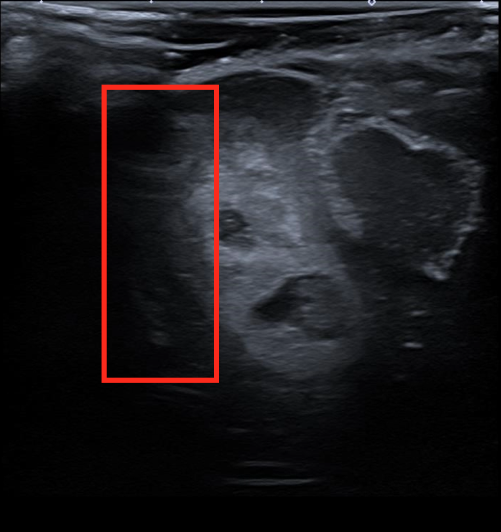
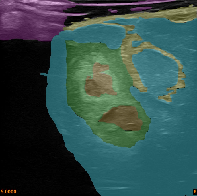
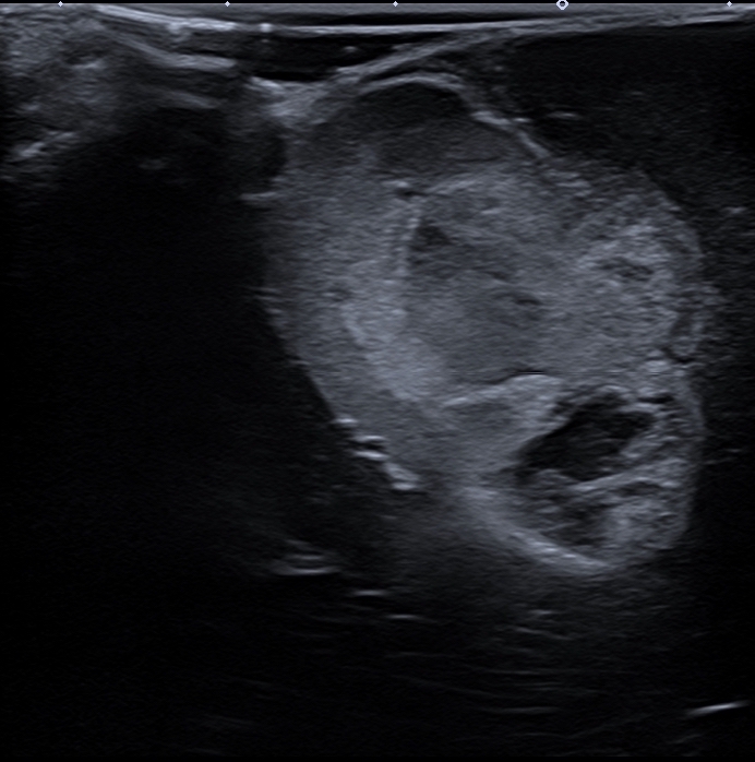
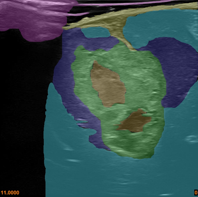
Figure 1: Ultrasound segmentation of iUS images. The top row shows suboptimal US image capture, the bottom row shows good US image capture. Annotations: green = solid tumour, orange = tumour necrotic core, yellow = cerebral sulci, dark blue = oedema, turquoise = surrounding normal brain, yellow = coupling fluid/probe brain interface.

Recent advances in iUS systems have raised interest in US image quality analysis. For example, the detection of bone shadow artefacts is a useful tool in orthopedic procedures. This can be segmented using handcrafted feature extraction techniques [4] and recently, deep learning approaches [5, 6, 7]. A similar application, but for rib shadow has been presented in [8]. The detection of AS has also been proposed for intravascular US [9, 10]. Generalized AS segmentation methods focusing on different organs and causes of AS, have been proposed [11, 12, 13, 14, 15]. The main challenge with these general segmentation methods is that they do not present outputs that can guide probe pose adjustment, as their methods do not uniquely identify shadowing that directly correlates to issues relating to the probe’s contact with the tissue. To address this limitation, the algorithm in [16] produces an US signal attenuation confidence map which has been shown to be able to guide surgical robotic systems using visual servoing [17, 18, 19]. The limiting factor for the above method is the a priori assumption that all distinct hyperechoic (i.e high intensity) lines correlate with reduced signal attenuation. However, in the case of anatomy such as brain, this not a valid assumption, as the convolutions and layered different tissues inherently create boundaries of acoustic impedance, that do not reduce signal attenuation. In this work, we propose a method for automatically detecting and topologically representing the visible tissue in US images - specifically for brain surgery. Our proposed method offers an advantage over previous work by eliminating assumptions concerning ultrasound signal attenuation in tissue, particularly in relation to hyperechoic features and signal penetration depth. Also, the method is robust to noise and disturbances in the US images. Our contributions are as follows:
1) a method for detecting visible tissue within US images using iterative smoothing filters - that does not rely on assumptions about signal attenuation in tissue
2) a method for topologically representing the visible tissue, which discretises the tissue information
3) a method for classifying scan lines affected by contact-related AS artefacts - where our performance evaluation shows the proposed method is state of the art. Using this information, operators can adjust the US probe’s position and pose to remove AS.
4) a framework for defining and representing confidence of the perceptual salience in US images, using the topological representation of the visible tissue, which can be used to support probe placement and pose adjustments for the improving of the US image quality.
We believe that by directly addressing the problem of probe-tissue contact quality assessment, the proposed algorithm can be used both to assist clinical training and optimise robot-assisted tissue scanning.

2 Methodology

The aim of the proposed method is the detection and the topological representation of the visible tissue which is not obscured by AS, within an US image $I\in\mathbb{R}^{300\times 600}$ - specifically tailored for application in brain surgery, where brain tissue contains large variations in pixel intensities and spatial features. This method processes the images with the aim to highlight areas of dynamic change in spatial image intensity, where then the topological representation can be constructed. From the topology of the visible tissue, areas affected by shadowing are detected and a confidence map of the perceptual salience is built. The overview of this process is shown in Fig. 2.

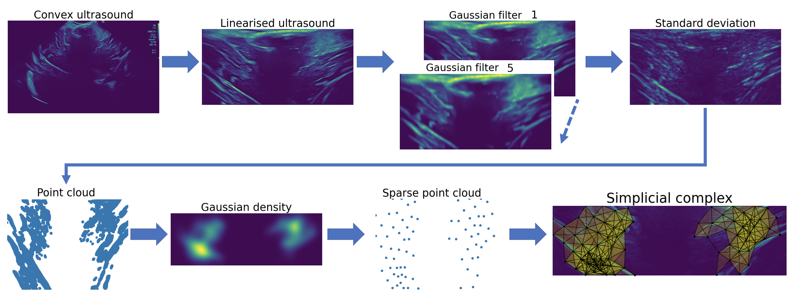
Figure 2: System flow diagram with visual example.

To detect areas of spatial intensity variation, we iteratively process the US image using Gaussian filters, with a vertical bias following Eq. 1.

$$G_{f}=h_{1}*G_{f-1},$$ (1)

$$h_{1}=(\nicefrac{{1}}{{\sqrt{2\pi\sigma_{u}}e^{-\nicefrac{{u^{2}}}{{2\sigma_{u}^{2}}}}}})(\nicefrac{{1}}{{\sqrt{2\pi\sigma_{v}}e^{-\nicefrac{{v^{2}}}{{2\sigma_{v}^{2}}}}}}),$$

$$\sigma_{u}=1.8,\sigma_{v}=0.2,f=[2..6],G_{1}=I$$

where, $G\in\mathbb{R}^{300\times 600}$ denotes an output of the Gaussian filter, $f$ indexing the iteration, $u,v$ are the image coordinates and $\sigma$ denotes the standard deviation of the Gaussian filter stack. The Gaussian smoothing is biased vertically, as the anatomical changes seen in brain US images are more likely to be exposed in the vertical direction. Other filters can be used, such as the median filter, to accomplish a similar effect. However, the Gaussian filter was chosen as it provides a smoother response. The purpose of the filter is the detection of areas of varying intensity. Therefore, the algorithm does not rely on specific levels of intensity, rather, on the rate of change in intensity. Introducing robustness to noise, prevalent in US images. Each output $G_{f}$ from the Gaussian filter sequence is stacked and the standard deviation is taken for each pixel across the stack using Eq. 2.

$$S_{u,v}=\sqrt{\frac{\sum_{f=1}^{6}(G_{f,u,v}-\frac{\sum_{f=1}^{6}G_{f,u,v}}{6})^{2}}{6}}$$ (2)

Where $S\in\mathbb{R}^{300\times 600}$ is the output of the standard deviation.

Image points with high spatial variation correspond to areas which have been affected the most by the smoothing process. Hence, these points are detected by thresholding the standard deviation output following Eq. 3 - where the threshold is defined as a percentage of the max range of pixel intensity (assumed 255 for grayscale).

$${\mathchoice{\raisebox{0.0pt}{$\displaystyle\chi$}}{\raisebox{0.0pt}{$\textstyle\chi$}}{\raisebox{0.0pt}{$\scriptstyle\chi$}}{\raisebox{0.0pt}{$\scriptscriptstyle\chi$}}}=\{(u,v)\mid S_{u,v}\geq\gamma\},\gamma=4$$ (3)

The points of high spatial variation are represented as a 2D point cloud $\textstyle\chi$. To reduce the computational load for building the topology, we sparsify the 2D point cloud using a Gaussian density map $\lambda\in\mathbb{R}^{300\times 600}$ defined in Eq. 4.

$$\lambda=\phi_{1}+\phi_{2}(1-h_{2}*S),$$ (4)

$$h_{2}=(\frac{1}{2\pi\sigma_{w}^{2}}e^{-\frac{u^{2}+v^{2}}{2\sigma_{w}^{2}}}),$$

$$\phi_{1}=15,\phi_{2}=20,\sigma_{w}=20$$

We then iterate through the point cloud, repeating Eq. 5 until all points are separated by their corresponding $\lambda_{a}$ distance threshold.

$${\mathchoice{\raisebox{0.0pt}{$\displaystyle\chi$}}{\raisebox{0.0pt}{$\textstyle\chi$}}{\raisebox{0.0pt}{$\scriptstyle\chi$}}{\raisebox{0.0pt}{$\scriptscriptstyle\chi$}}}-A,A:=\{d\subseteq{\mathchoice{\raisebox{0.0pt}{$\displaystyle\chi$}}{\raisebox{0.0pt}{$\textstyle\chi$}}{\raisebox{0.0pt}{$\scriptstyle\chi$}}{\raisebox{0.0pt}{$\scriptscriptstyle\chi$}}}\mid\forall a,b\in d:dist(a,b)\leq\lambda_{a}\}$$ (5)

Where, $a,b$ indexes elements in the point cloud set and $dist()$ gives the euclidean distance between two points (pixels). To generate the topology of the visible tissue, a Vietoris–Rips complex [20] is then constructed on the sparse point cloud, defined in Eq. 6.

$$\Psi:=\{d\subseteq{\mathchoice{\raisebox{0.0pt}{$\displaystyle\chi$}}{\raisebox{0.0pt}{$\textstyle\chi$}}{\raisebox{0.0pt}{$\scriptstyle\chi$}}{\raisebox{0.0pt}{$\scriptscriptstyle\chi$}}}\mid\forall a,b\in d:dist(a,b)\leq\epsilon\},\epsilon=60$$ (6)

Where, $\epsilon$ defines the maximum distance threshold. The Vietoris–Rips complex method was chosen over alternatives such as the Delaunay complexes due to its simplicity and also the robustness to outliers. This choice was also influenced by its use in persistent homology [21].

For every group of 3 points within a predefined distance, this topological representation forms 2D simplexes (triangles) $\Delta:=\{\delta:\delta\in\Psi\}$. For each scan line $\xi_{sl},sl=[1..600]$ on the US image, the method will assign a single binary classification, $1$ for AS and $0$ for visible tissue. One classification label per scan line is used because contact-related AS affects an entire scan line. For every image pixel, the number of overlapping 2D simplexes are counted, creating an occurrence map $O$. We define that there is contact-related AS, along a single scan line $\xi_{sl}$, if the number of overlapping 2D simplexes $\forall\delta\in\Delta$ (over the scan line) is lesser than threshold $\tau$. This insufficient topological representation along a scan line is defined as the presence of AS. The justification for this is that an area of AS may not appear distinct nor uniform as AS can be variable in its margins, shape, and extent, due to the uneven texture feature of the tissue scanned and the frequent presence of confounding factors, such as brain sulci, blood products, or calcification. For example, an image may contain a hyperechoic brain sulci protrusion into the AS area.

The output produced is a vector of length $600$, corresponding to the width of the image. The confidence map is a pixel wise quantification of the confidence of the perceptual salience, which represents the resolution and contrast of the detected visible tissue. A high score indicates high quality tissue contrast and resolution. The confidence map is constructed by taking the log of the occurrence map, $\hat{M}=log(O+1)$.

3 Experimental Setup

3.1 Data

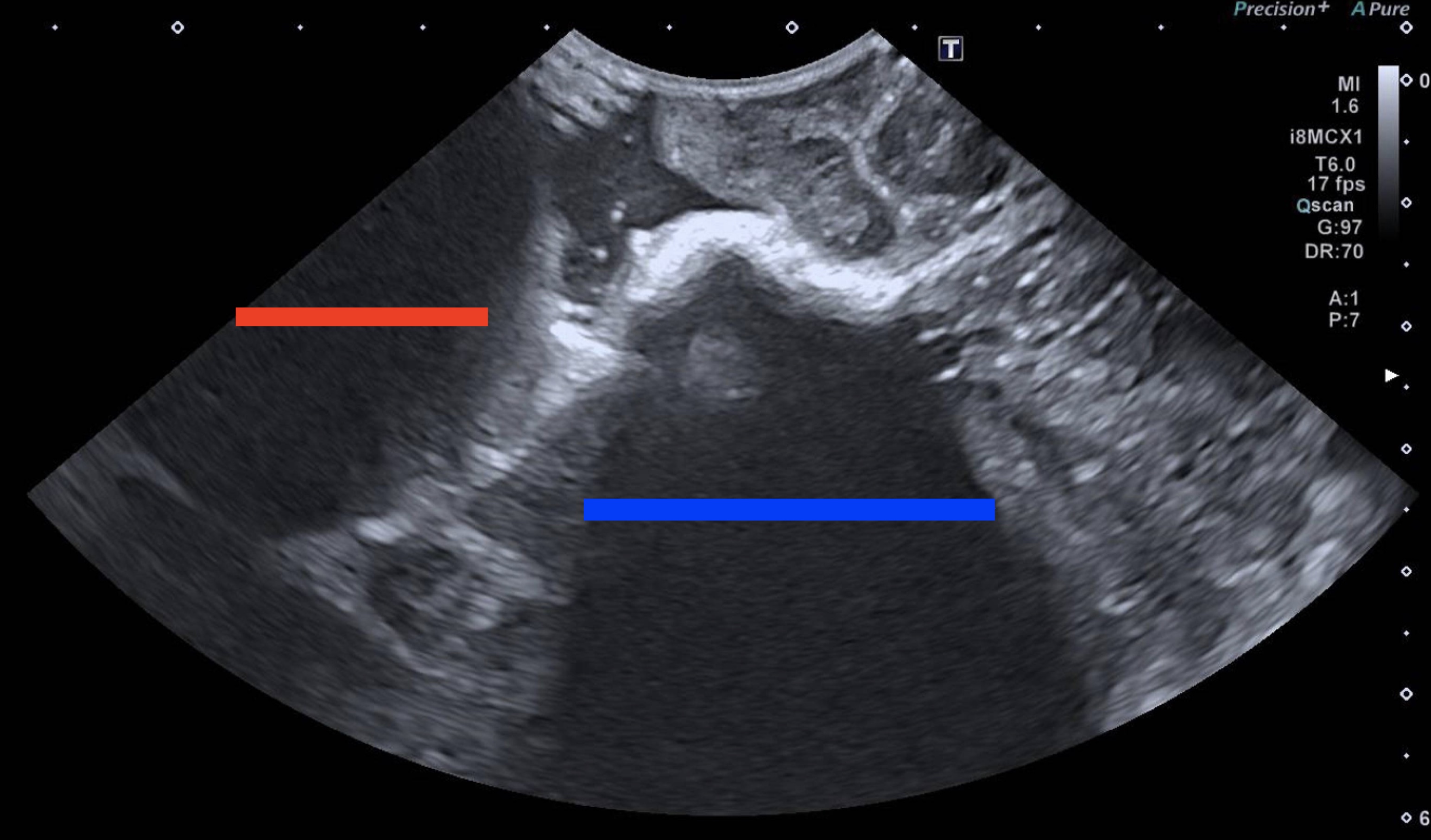
Figure 3: Sample annotations. The red line delineates AS secondary to poor contact whilst the blue line defines AS related to other causes (in this case echogenic blood clot in a resection cavity).

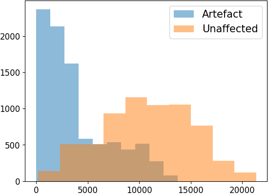
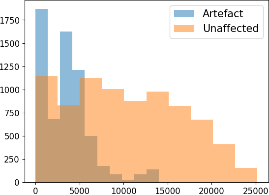
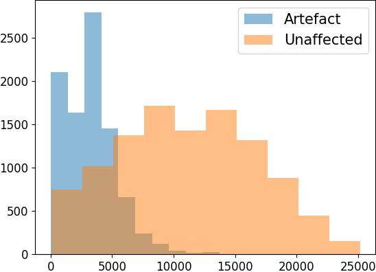
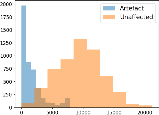
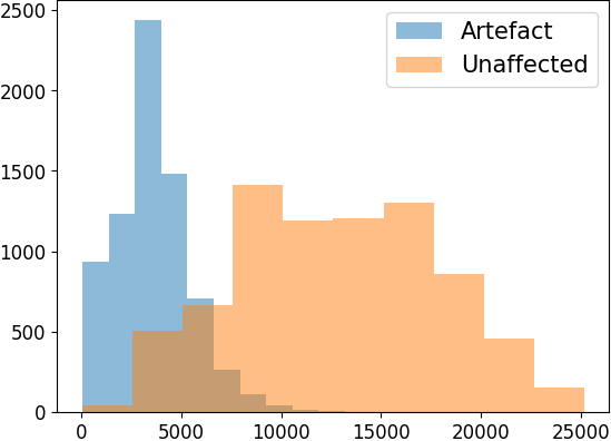
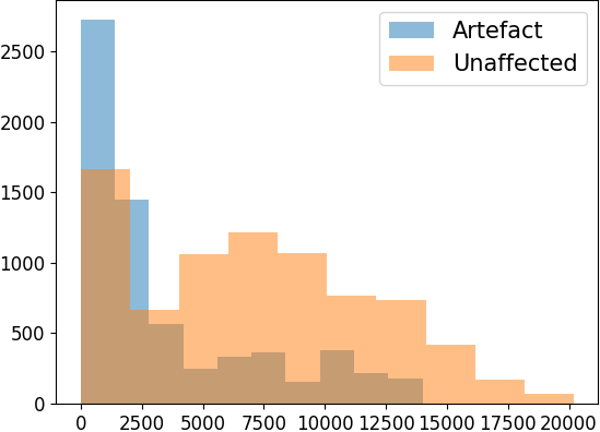
Figure 4: The distributions of the scanline sum of pixel intensities for each fold. The left column displays the seen data, the right the unseen. The top row is fold 1, middle fold 2 and third fold 3. The x axis is the scanline sum of pixel intensities. The y axis is the occurrence.

For the evaluation of the proposed AS detection method a dataset containing 51 images from eleven different patients was collected. Sourced from routine pseudo-anonymised 2D US images, acquired during neurosurgery, using a Canon i900 US machine (where the US probe is sheathed with a sterile Polyethylene probe cover - with US gel added) and both a linear and convex probe, at Imperial College NHS healthcare trust, London, retrospectively reviewed by a consultant neuroradiologist experienced in neuro-oncological iUS. The images exhibit varying degrees of AS artefact secondary to poor probe-tissue contact. The AS annotations were manually done using the CVAT [22]. The study had full local ethical approval by HRA and Health and Care Research Wales (HCRW) auhorities. Study title - US-CNS: Multiparametric Advanced Ultrasound Imaging of the Central Nervous System Intraoperatively and Through Gaps in the Bone, IRAS project ID: 275556, Protocol number: 22CX7609, REC reference: 22/WA/0259, Sponsor: Research Governance and Integrity Team (RGIT). For standardisation, all convex images were manually linearised. For performance evaluation, 3-fold cross-validation was used - the dataset is split into a seen and unseen subset, with the division done on the patient level. The first fold contained 27 seen images and 24 unseen. The second, 33 seen and 18 unseen. The third, 26 seen and 25 unseen. The breakdown of the 51 images [patient:#images] [1:1, 2:3, 3:3, 4:4, 5:9, 6:5, 7:6, 8:1, 9:8, 10:4, 11:7]. Example US images and annotations are displayed in Fig. 3. The distributions of the scanline sum of pixel intensities for each fold are displayed in Fig. 4 - highlighting the differences of each fold (seen and unseen) and the validity of the 3-fold evaluation.

As the confidence values are in themselves arbitrary - where a good scan in a position where tissue visibility is poor may result in low confidence. The evaluation of the confidence map behaviour can only be achieved by measuring how the confidence values change as a probe’s pose is intentionally positioned in and out of optimality. For this, two phantoms were scanned over by an experienced neurosurgeon. The scanning involved a simple tilt of the probe, starting from -90°$>$ perpendicular $>$ +90°with respect to the tissue surface. The Zonare Z.one US system with a C4-1 transducer was used and data was recorded via an Epiphan DVI2USB 3.0 frame grabber. Scans 1-4 used the FAST/Acute Abdomen Phantom ”FAST/ER FAN” [23] - where scan 1 and 2 were taken from the abdomen, 3 from the rib cage and 4 from the kidney. Scan 5 used a Kezlex brain phantom [24], reproducing some of the echogenic features (although without the distinction between sulci and gyri) and the ventricles. Frames were extracted using FFmpeg, at a rate of $10Hz$.

3.2 Performance evaluation setup

For the evaluation of the AS classification, our proposed method (Topol) is compared to a scan line intensity method (Thresh) and a modified VGG16 model (VGG16) [25]. As no existing methods are suitable for comparison, Thresh and VGG16 were used for comparison to cover both simple statistical and deep learning approaches - the specific choice of the Thresh method was motivated by [9] [10] and the use of the VGG16 architecture was motivated by [15]. A confusion matrix is used for the quantitative analysis, where a positive classification denotes a scanline effected by AS. The methods are compared in terms of Accuracy (ACC), Specificity (TNR), Sensitivity (TPR) and Precision (PPV). Where: True positive $TP$, true negative $TN$, false positive $FP$, false negative $FN$, $ACC=(TP+TN)/(TP+TN+FP+FN)$, $TNR=TN/(TN+FP)$, $TPR=TP/(TP+FN)$, $PPV=TP/(TP+FP)$.

Parameter tuning for Topol, namely, $[f,\sigma_{u},\sigma_{v},\sigma_{w},\phi_{1},\phi_{2},\epsilon]$, is done using the seen subset exclusively. The best performing set of parameters for Topol - found using a manual grid search - was identical across the 3 folds and as described in Sec. 2. With the exception of the Gaussian filter where fold 1 and 3 used $\sigma_{v}=0.2$, fold 2 used $\sigma_{v}=0.3$. This capability to manually make small adjustments is a benefit as it enables flexibility and broader application. The scanline threshold was constant for all folds $\tau=2$. Thresh individually classifies each scan line using the sum of the scan line and a fixed threshold $\sum_{i=1}^{300}\xi_{sl}>\kappa$. The threshold is determined using a receiver operating characteristic curve (ROC) on the seen data. Namely - $\kappa=[4900,5000,5500]$. Due to the limited data available for training, and the expected large distribution shift from natural scenes to ultrasound images, we chose to perform linear probing using a frozen pretrained VGG16 feature encoder (ImageNet [26]) rather than fine tuning [27]. Gradient descent is performed, for 10 epochs, on a classification head. The pseudo code for this architecture is: $Featureencoder>Linear(ch=600)>ReLU>Concat((Img,600),0)>Conv1d(ch=1)>Sigmoid>Output$ where, $Output\in\mathbb{R}^{600}$ and $ch$ denotes the output channel size. We used the best performing checkpoints on the unseen/validation dataset, obtained from epochs $[7,9,9]$. To reduce the influence of the US gel artefact, the top 100 rows are cropped from all US images, for all methods at the point of input. The choice of 100 rows was based on observations of the dataset and the average maximum point where the gel artefact ended. This parameter was varied for assessment and it was noted that similar performance was achievable with greatly reduced or no cropping. We recommend this step for methods working explicitly with the visible tissue within US images, as any parameter calibration or data learning on images containing gel artefact may result in vulnerable dependence on an extraneous feature. Based on the annotator’s experience, it is recommended that both clinicians and algorithms should not rely on the gel artefact.

For the confidence map evaluation, our proposed method is compared with the random walk method [16] (Random walk) - using the official MATLAB code and default parameters alpha = 2.0; beta = 90; gamma = 0.03. The Topol parameters tuned on fold 1 of the AS classification were used. We assume that the ideal confidence trajectory should follow a normal distribution, and evaluate it using the root mean squared error, $RMSE=\sqrt{1/n\Sigma_{i=1}^{n}{(T_{i}-\hat{T}_{i})^{2}}},\hat{T}_{i}=mean(\hat{M}_{i})$. Where $T$ is the target vector - normal distribution fitted to the max and min of $\hat{M}$ - $n$ is the number of frames in the scan video.

The code was implemented on an Intel i7 CPU 3.80GHz and NVIDIA GeForce 3080 using Python. For compatibility with real time control systems and integration into a robotic framework, the algorithm was also implemented (with minimal optimisation) in C++ and executed at 20Hz.

4 Results and Discussion

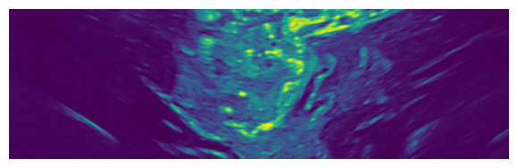
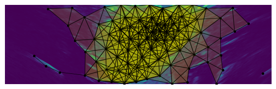
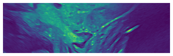
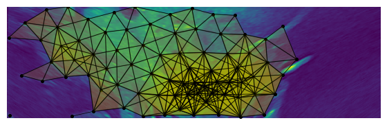
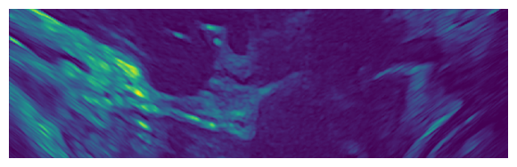
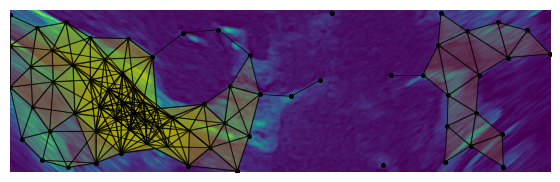
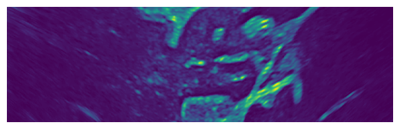
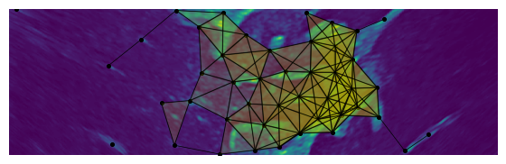
Figure 5: Sample simplicial complex outputs.

Sample simplicial complex outputs are displayed in Fig. 5. What can be observed is the lack of triangles on areas affected by AS, and the concentration of triangles on areas with high spatial variation.

4.1 Scan line classification

Table 1: Scan line classification results. A positive sample corresponds to a scan line affected by AS. Acronyms: True positive $TP$, true negative $TN$, false positive $FP$, false negative $FN$, accuracy $ACC$, sensitivity $TPR$, specificity $TNR$ and precision $PPV$.

Fold 1	Algo	$ACC$	$TNR$	$TPR$	$PPV$
	Thresh	0.89	0.89	0.89	0.87
Seen	VGG16	0.90	0.91	0.92	0.90
	Topol	0.90	0.95	0.85	0.93
	Thresh	0.82	0.82	0.82	0.79
Unseen	VGG16	0.79	0.79	0.78	0.76
	Topol	0.85	0.87	0.83	0.84

Fold 2	Algo	$ACC$	$TNR$	$TPR$	$PPV$
	Thresh	0.84	0.84	0.83	0.81
Seen	VGG16	0.91	0.92	0.90	0.90
	Topol	0.87	0.93	0.80	0.90
	Thresh	0.89	0.87	0.92	0.86
Unseen	VGG16	0.92	0.95	0.89	0.94
	Topol	0.91	0.97	0.85	0.96

Fold 3	Algo	$ACC$	$TNR$	$TPR$	$PPV$
	Thresh	0.89	0.92	0.87	0.91
Seen	VGG16	0.90	0.92	0.88	0.91
	Topol	0.90	0.96	0.84	0.96
	Thresh	0.81	0.73	0.93	0.73
Unseen	VGG16	0.78	0.73	0.85	0.71
	Topol	0.85	0.85	0.84	0.81

Avg	Algo	$ACC$	$TNR$	$TPR$	$PPV$
	Thresh	0.87	0.88	0.86	0.86
Seen	VGG16	0.90	0.92	0.90	0.90
	Topol	0.89	0.95	0.83	0.93
	Thresh	0.84	0.81	0.89	0.79
Unseen	VGG16	0.83	0.82	0.84	0.80
	Topol	0.87	0.90	0.84	0.87

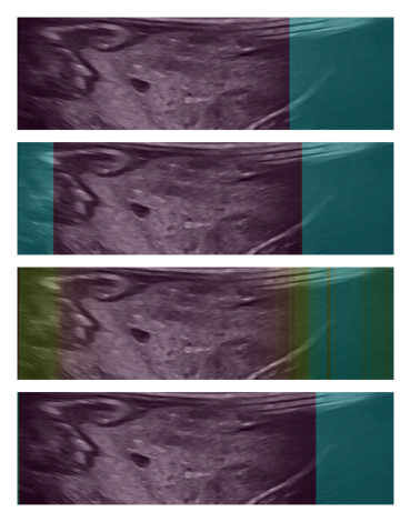
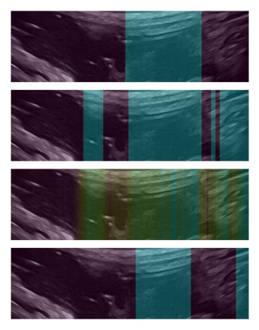
Figure 6: AS detection on two US images. The top row shows the annotation, second is from Thresh, third is from VGG16 and bottom is from Topol. The cyan areas are detected AS, the green areas are areas of volatile classification.

The results of the scan line classification are presented in Tab. 1 and Fig. 6. The key results from the table are on the unseen dataset, as these results show the robustness to distribution shift. It can be first determined that Topol is the most robust method to distribution shift with more consistent performance between seen and unseen data. Second, the results produced by Thresh show that over-reliance on pixel intensities leads to over-sensitivity. Both examples in Fig. 6 highlight the significance of over sensitivity. In Fig. 6 example 2 (right column), Thresh and VGG16 estimate that most of the image is affected by shadow - even where there are clearly defined tissue structures. In example 1 (left column), both Thresh and VGG16 incorrectly predict that the left side of the image is affected by shadow. This could lead to erroneous pose correction to non existing shadowing. Third, the outputs of VGG16 in Fig. 6 show areas of green, which correspond to areas of classification volatility. Highlighting the difficulty of attaining sufficient generalisation - especially emphasising the issue of small data availability which is the case in this problem, and therefore the need for non data learning methods. Also, the lack of explainability and the interpretability of it’s behaviour and output is a significant problem. Although deep learning has in many applications of computer vision surpassed traditional techniques, this is entirely dependant on the availability of enormous volumes of relevant data, and that the achieved performances can be substantial enough to distract from the typical black box reliability issues. While the Topol method relies on parameters that need calibration - which could be optimised automatically using methods such as grid search - this enables the algorithm to be flexible to new implementation setups, and an intuitive understanding for the process. From the results, it can be concluded that Topol is able to generalise successfully to small datasets and produces state of the art results.

4.2 Confidence map estimation and US probe pose analysis

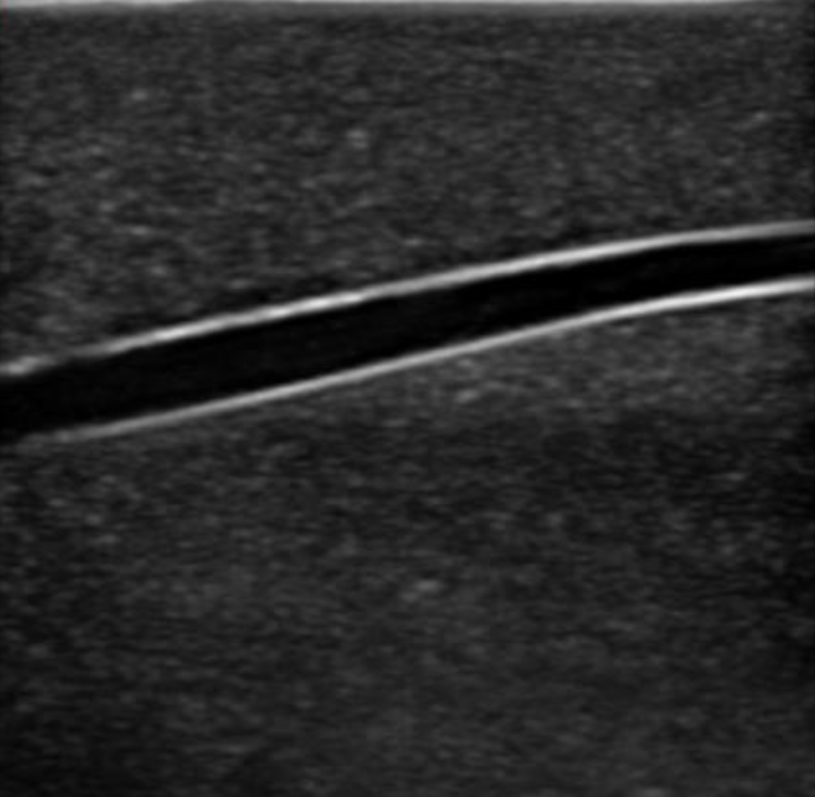
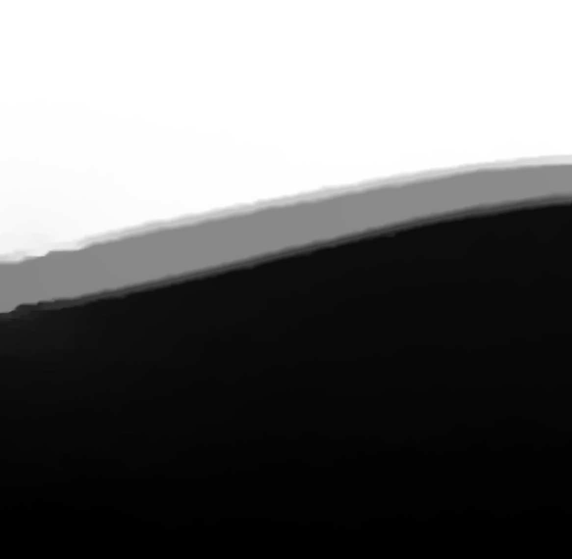
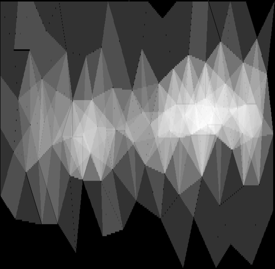
Figure 7: This example shows the affect of strong line features on the confidence maps produced using Random walk (middle) and Topol (right).

Qualitative assessment of the confidence maps generated with Random walk and Topol was done using a sample image of the CAE Blue Phantom’s Pediatric 4 Vessel US Training Block [28], with the vessel filled with a simulated blood solution. These results demonstrate the algorithmic responses to hyperechoic physiology commonly found in the brain, that may visually appear similar to bone — which would be an improbable scenario in neurosurgery. The result for Random walk is highly influenced by the bright horizontal lines as shown in Fig. 7. This highlights the consequence of correlating hyperechoic lines with signal attenuation. Whereas, Topol produces high confidence around the, non shadowing, fully visible blood vessel. Furthermore, as the output of Random walk is continuous, the process for determining any thresholds is ambiguous.

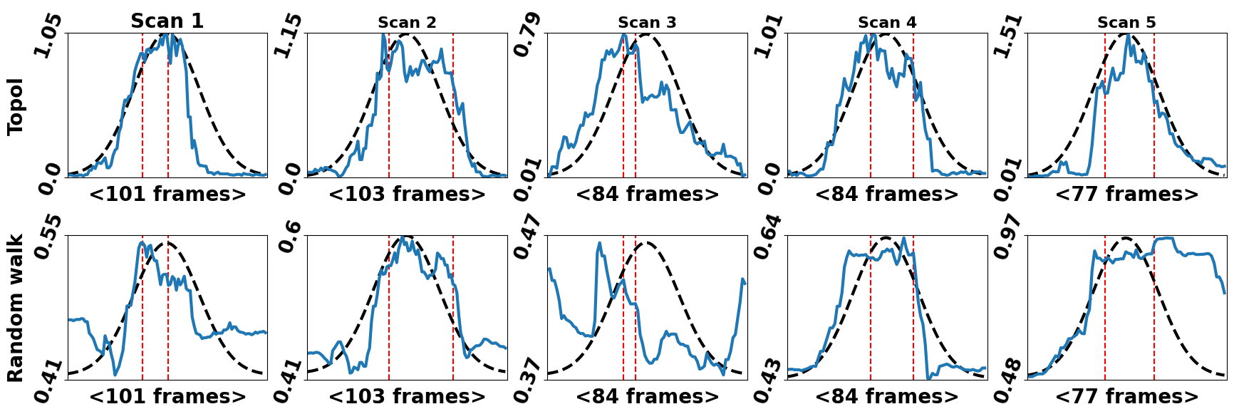
Figure 8: The per frame average confidence vector outputs - y axis = frames and x axis = average confidence. The blue lines show the method’s outputs, Topol top row and Random walk bottom row. The black dotted lines are the scaled normal curve. The dotted red lines are where the annotators perceived best images are. Corresponding RMSE results are shown in the table.

Method	Scan 1	Scan 2	Scan 3	Scan 4	Scan 5
Topol	0.19	0.15	0.22	0.14	0.17
Random walk	0.24	0.17	0.44	0.15	0.41

Figure 9: The method’s RMSE results are shown for each scan. In all cases Topol produces the best results.

An experiment of the usability of the compared methods for pose analysis was done using the abdomen and brain phantom data described in Sec. 3.1. Based on [29], $mean(\hat{M})$ is used to determine the confidence per frame. For the ground truth, we make the assumption that as the probe tilts on the spot, the mean confidence, $\hat{T}$, should behave like a normal distribution curve $T$, with confidence peaking around the middle frame of the sequence (probe perpendicular to the tissue) and low confidence at the start and end. Each target curve is fitted to the max and min of $\hat{T}$ for each scan. Fig. 8 and Tab. 9 shows the results. This assumed normal curve behaviour was ensured by the operator - the data was collected in such a way that perpendicularity produced the best images and the further from it the worse the images became - and also the optimal range of images were chosen from the videos and are highlighted using the vertical red dotted lines. This assumption is logical for brain surgery due to the convex shape. Quantitative analysis is performed by measuring the RMSE of the $\hat{T}$ vector (blue line) against the fitted normal curve (black dotted line). Fig. 8 shows that for all scans, the behaviour of Topol is closer to what is expected. The range of $\hat{T}$ values provided by Topol can also be regarded as more intuitive than Random walk as the confidence is starting near 0 and peaking around 1.

4.3 Robustness to Parameter Perturbations

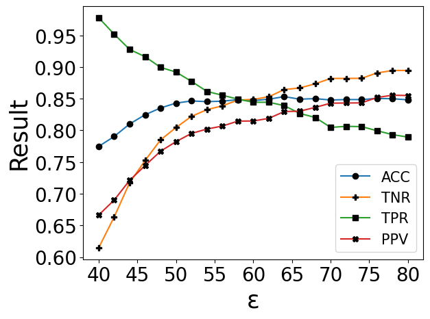
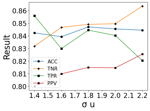
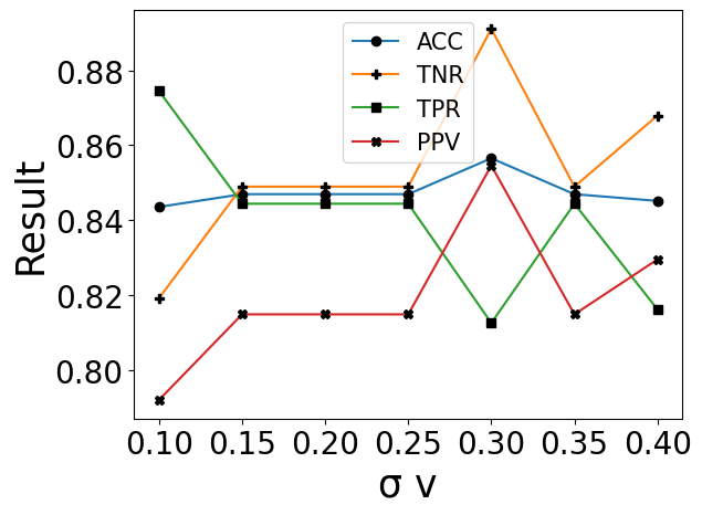
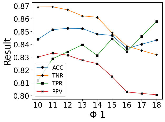
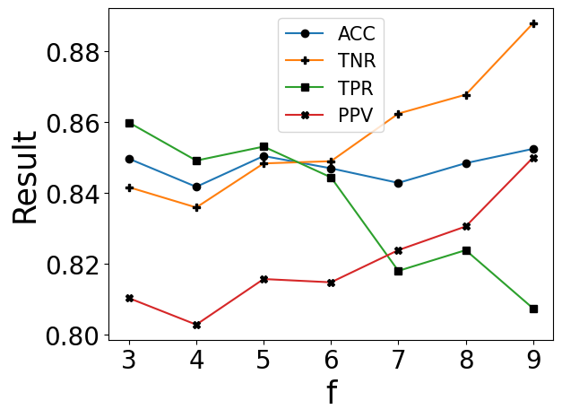
Figure 10: Graphs displaying the effect of individually varying the parameters on the performance of the whole system - using the unseen fold 3 data. The blue lines = ACC, orange lines = TNR, green lines = TPR and red lines = PPV.

The use of hand crafted features and parameter calibrations introduces uncertainty regarding the robustness of these manually determined components. To assess how the algorithm performs under varying parameters, we conduct an experiment using the unseen data from fold 3 and perturb individual parameters to evaluate the impact on the overall performance. The results of this experiment are shown in the graphs in Fig. 10. What can be observed is the largely minimal effect of an individually drifting parameter on the overall system - where most metrics across the different parameter graphs produce results remaining above 0.8. This is evidence of the robustness of the design of the algorithm, because the performance is maintained under parameter uncertainty. The most sensitive parameter to change is $\epsilon$. This is a logical outcome as $\epsilon$ determines the triangulation conditions of the point cloud, and a small $\epsilon$ value would indicate extreme tissue anatomy variation - which is unlikely. The range of parameters chosen for this experiment were decided based on what was believed reasonable.

5 Conclusion

Our paper introduces a novel topological analysis-based approach for the detection of contact related AS and confidence of the perceptual salience of the detected visible tissue. The proposed algorithm first processes the image using iterative Gaussian filters, to expose areas of high resolutions. A 2D point cloud is constructed and sparsified using a density weighting. A 2D Vietoris-Rips complex is finally constructed, which represents the topology of the underlying tissue structure within the US image. Evaluation of AS scan line classification and confidence behaviour has been performed. In both cases, the proposed method outperforms the compared methods. We believe that the dual classification of scan lines affected by AS and also the generation of the confidence maps is a new framework that can be used to support automated robotic solutions to intraoperative ultrasound scanning of the brain and also teach and support sonographers and neurosurgeons.

We acknowledge that the limited AS dataset influences the robustness of the evaluation process. However, this highlights the need for non data-driven methods for this application, as the data is difficult to collect and requires niche expertise to annotate. For future work, we do aim to collect and annotate more data. Further, we will be looking to integrate this method into a visual servoing setup using a prototypical DLR Miro surgical robotic arm [30], where continued optimisation of the C++ implementation will be made. Continued algorithmic development will also be pursued, firstly to integrate the US machine’s parameter settings into the algorithm. Secondly, to specifically evaluate how the method handles narrow-focused shadowing which would likely be caused by small gas bubbles. Thirdly, explore other potential applications of this method, perhaps onto different organs and the detection of different types of shadowing.

5.0.1 Acknowledgements

This project was supported by UK Research and Innovation (UKRI) Centre for Doctoral Training in AI for Healthcare (EP/S023283/1), the Royal Society (URF$\setminus$R$\setminus$2 01014), the NIHR Imperial Biomedical Research Centre.

References

- [1] J. M. K. Mislow, A. J. Golby, and P. M. Black, “Origins of intraoperative mri.” Magnetic resonance imaging clinics of North America, vol. 18 1, pp. 1–10, 2010.
- [2] R. A. Sastry, W. L. Bi, S. D. Pieper, S. F. Frisken, T. Kapur, W. M. Wells, and A. J. Golby, “Applications of ultrasound in the resection of brain tumors,” Journal of Neuroimaging, vol. 27, 2017.
- [3] L. Dixon, A. Lim, M. Grech-Sollars, D. Nandi, and S. J. Camp, “Intraoperative ultrasound in brain tumor surgery: A review and implementation guide,” Neurosurgical Review, vol. 45, pp. 2503 – 2515, 2022.
- [4] F. Berton, F. Cheriet, M.-C. Miron, and C. Laporte, “Segmentation of the spinous process and its acoustic shadow in vertebral ultrasound images,” Computers in biology and medicine, vol. 72, pp. 201–11, 2016.
- [5] A. Z. Alsinan, V. M. Patel, and I. Hacihaliloglu, “Bone shadow segmentation from ultrasound data for orthopedic surgery using gan,” International Journal of Computer Assisted Radiology and Surgery, vol. 15, pp. 1477 – 1485, 2020.
- [6] P. Wang, M. Vives, V. M. Patel, and I. Hacihaliloglu, “Robust bone shadow segmentation from 2d ultrasound through task decomposition,” in MICCAI, 2020.
- [7] A. Rahman, J. M. J. Valanarasu, I. Hacihaliloglu, and V. M. Patel, “Simultaneous bone and shadow segmentation network using task correspondence consistency,” in MICCAI, 2022.
- [8] S. M. Ravishankar, R. Tsumura, J. W. Hardin, B. Hoffmann, Z. Zhang, and H. K. Zhang, “Anatomical feature-based lung ultrasound image quality assessment using deep convolutional neural network,” 2021 IEEE International Ultrasonics Symposium (IUS), pp. 1–4, 2021.
- [9] E. dos Santos Filho, Y. Saijo, T. Yambe, A. Tanaka, and M. Yoshizawa, “Segmentation of calcification regions in intravascular ultrasound images by adaptive thresholding,” 19th IEEE Symposium on Computer-Based Medical Systems (CBMS’06), pp. 446–454, 2006.
- [10] J. H. Lee, G. Y. Kim, Y. N. Hwang, and S. M. Kim, “Automatic detection of dense calcium and acoustic shadow in intravascular ultrasound images by dual-threshold-based segmentation approach,” Sensors and Materials, 2018.
- [11] P. Hellier, P. Coupé, X. Morandi, and D. L. Collins, “An automatic geometrical and statistical method to detect acoustic shadows in intraoperative ultrasound brain images,” Medical image analysis, vol. 14 2, pp. 195–204, 2010.
- [12] S. Yasutomi, T. Arakaki, and R. Hamamoto, “Shadow detection for ultrasound images using unlabeled data and synthetic shadows,” arXiv: Image and Video Processing, 2019.
- [13] Q. Meng, C. F. Baumgartner, M. Sinclair, J. Housden, M. Rajchl, A. Gómez, B. Hou, N. Toussaint, J. Tan, J. Matthew, D. Rueckert, J. A. Schnabel, and B. Kainz, “Automatic shadow detection in 2d ultrasound,” 2018.
- [14] Q. Meng, J. Housden, J. Matthew, D. Rueckert, J. A. Schnabel, B. Kainz, M. Sinclair, V. A. M. Zimmer, B. Hou, M. Rajchl, N. Toussaint, O. Oktay, J. Schlemper, and A. Gomez, “Weakly supervised estimation of shadow confidence maps in fetal ultrasound imaging,” IEEE Transactions on Medical Imaging, vol. 38, pp. 2755–2767, 2019.
- [15] V. Melapudi, C. Aladahalli, K. S. Shriram, and H.-M. Chang, “Exploiting acquisition path to detect shadows in ultrasound images,” in Medical Imaging, 2022.
- [16] A. Karamalis, W. Wein, T. Klein, and N. Navab, “Ultrasound confidence maps using random walks,” Medical image analysis, vol. 16 6, pp. 1101–12, 2012.
- [17] P. Chatelain, A. Krupa, and N. Navab, “Confidence-driven control of an ultrasound probe,” IEEE Transactions on Robotics, vol. 33, pp. 1410–1424, 2017.
- [18] Z. Jiang, M. Grimm, M. Zhou, J. Esteban, W. Simson, G. Zahnd, and N. Navab, “Automatic normal positioning of robotic ultrasound probe based only on confidence map optimization and force measurement,” IEEE Robotics and Automation Letters, vol. 5, pp. 1342–1349, 2020.
- [19] K. Li, J. Wang, Y. Xu, H. Qin, D. Liu, L. Liu, and M. Q. Meng, “Autonomous navigation of an ultrasound probe towards standard scan planes with deep reinforcement learning,” 2021 IEEE International Conference on Robotics and Automation (ICRA), pp. 8302–8308, 2021.
- [20] S. Lim, F. Mémoli, and O. B. Okutan, “Vietoris-rips persistent homology, injective metric spaces, and the filling radius,” ArXiv, vol. abs/2001.07588, 2020.
- [21] H. Edelsbrunner and J. Harer, “Persistent homology — a survey.”
- [22] B. Sekachev, N. Manovich, M. Zhiltsov, A. Zhavoronkov, D. Kalinin, B. Hoff, TOsmanov, D. Kruchinin, A. Zankevich, DmitriySidnev, M. Markelov, Johannes222, M. Chenuet, a andre, telenachos, A. Melnikov, J. Kim, L. Ilouz, N. Glazov, Priya4607, R. Tehrani, S. Jeong, V. Skubriev, S. Yonekura, vugia truong, zliang7, lizhming, and T. Truong, “opencv/cvat: v1.1.0,” Aug. 2020. [Online]. Available: https://doi.org/10.5281/zenodo.4009388
- [23] K. Kagaku, “Fast/acute abdomen phantom ”fast/er fan”.” [Online]. Available: https://www.kyotokagaku.com/en/products_data/us-5/
- [24] Kezlex, “Skull and brain phantom - endoscopic for hydrocephalus.” [Online]. Available: https://www.kezlex.com/en/products/skull/a38/
- [25] K. Simonyan and A. Zisserman, “Very deep convolutional networks for large-scale image recognition,” in International Conference on Learning Representations, 2015.
- [26] J. Deng, W. Dong, R. Socher, L.-J. Li, K. Li, and L. Fei-Fei, “Imagenet: A large-scale hierarchical image database,” in 2009 IEEE conference on computer vision and pattern recognition. Ieee, 2009, pp. 248–255.
- [27] A. Kumar, A. Raghunathan, R. Jones, T. Ma, and P. Liang, “Fine-tuning can distort pretrained features and underperform out-of-distribution,” ArXiv, vol. abs/2202.10054, 2022.
- [28] C. Healthcare, “Pediatric 4 vessel ultrasound training block.” [Online]. Available: https://medicalskillstrainers.cae.com/pediatric-4-vessel-ultrasound-training-block/p?skuId=22
- [29] S. Virga, O. Zettinig, M. Esposito, K. Pfister, B. Frisch, T. Neff, N. Navab, and C. Hennersperger, “Automatic force-compliant robotic ultrasound screening of abdominal aortic aneurysms,” 2016 IEEE/RSJ International Conference on Intelligent Robots and Systems (IROS), pp. 508–513, 2016.
- [30] U. Seibold, B. Kübler, T. Bahls, R. Haslinger, and F. Steidle, “The DLR MiroSurge surgical robotic demonstrator,” ser. The Encyclopedia of Medical Robotics, J. P. Desai and R. V. Patel, Eds. WORLD SCIENTIFIC, October 2018, vol. 1, pp. 111–142.