Probing the limits of optical cycling in a predissociative diatomic molecule

Abstract

Molecular predissociation, the spontaneous nonradiative bond breaking process, can limit the ability to scatter a large number of photons required to reach the ultracold regime in laser cooling. Unlike rovibrational branching, predissociation is irreversible since the fragments fly apart with high kinetic energy. Of particular interest is the simple diatomic molecule, CaH, for which the two lowest electronically excited states used in laser cooling, $A^{2}\Pi_{1/2}$ and $B^{2}\Sigma^{+}$, lie above the dissociation threshold of the ground potential. In this work, we present measurements and calculations that quantify the predissociation probabilities $P_{\mathrm{pd}}$ affecting the cooling cycle. For the lowest vibrational levels, we find $P_{\mathrm{pd}}$ of $\sim 10^{-6}$ for $A(v^{\prime}=0)$ and $\sim 10^{-3}$ for $B(v^{\prime}=0)$. The results allow us to design a laser cooling scheme that will enable the creation of an ultracold and optically trapped cloud of CaH molecules. In addition, we use the results to propose a two-photon pathway to controlled dissociation of the molecules in order to gain access to their ultracold fragments, including hydrogen.

I Introduction

Rapid and repeated photon scattering is not only an efficient method of removing entropy from an atom or a molecule via photon recoils [1], but it also enables the high-fidelity single quantum state preparation and measurement needed for quantum information protocols [2, 3]. Optical cycling between the ground state and a low-lying electronic excited state, pioneered with SrF [4] and CaF [5, 6], has led to recent progress with laser cooled molecules such as tweezer arrays of CaF [7], a three-dimensional lattice of YO [8], magneto-optical trapping (MOT) of CaOH [9], and one-dimensional Sisyphus cooling of CaOCH₃ [10].

The primary challenge of direct laser cooling is the large photon budget necessary for bringing a cryogenically precooled molecular beam to within the MOT capture velocity [11, 12]. For example, typical molecular beams emanating from a cryogenic buffer gas beam (CBGB) source travel at mean forward velocities of $\sim 200$ m$/$s [13]. The recoil velocity per photon is $\sim 2$ cm$/$s, hence $>10^{4}$ photon scatters are needed to bring the molecular beam to a standstill. The photons must be scattered faster than $10^{6}$ s^-1 to accomplish slowing within a $\sim 1$ m distance. Satisfying these criteria can be challenging for molecules with complex internal structures. Indeed, alternative slowing schemes such as traveling wave Stark deceleration [14], the electro-optic Sisyphus effect [15], centrifuge deceleration [16], and Zeeman-Sisyphus slowing [17] have been demonstrated. These alternative schemes leverage state-dependent electric and magnetic field dependencies to remove entropy with minimal photon scatters. However, quantum-state resolved detection still requires optical cycling.

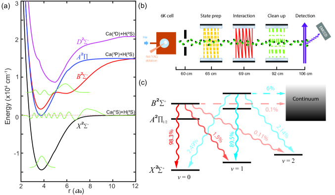
Figure 1: CaH molecular properties relevant to this work. (a) Potential energy surfaces (PES) for the 4 lowest electronic states: $X^{2}\Sigma^{+}$, $A^{2}\Pi$, $B^{2}\Sigma^{+}$, and $D^{2}\Sigma^{+}$. Spin-orbit interaction is omitted. The $x$-axis is the internuclear separation $r$ in Bohr radii ($a_{0}$) and the $y$-axis is energy in cm^-1 (1 cm${}^{-1}\approx$ 30 GHz). The energy origin is chosen as the Ca$(^{1}S)$+H$(^{2}S)$ continuum threshold ($v_{\mathrm{th}}$). Superimposed are the wavefunctions (bottom to top) for the $X(v^{\prime\prime}=0)$ absolute ground state, $X(v^{\prime\prime}=15)$ least-bound state, and $B(v^{\prime}=4)$ excited state. (b) Experimental layout used in this work. A buffer-gas cooled molecular beam emanates from the cryogenic cell and encounters 4 spatially separated regions: state preparation (S), interaction (I), cleanup (C), and detection (D). Each region includes multipassed lasers described in the text. The diagram is not aligned to scale. (c) Relevant vibrational branching ratios (squiggly arrows) calculated for the $B^{2}\Sigma^{+}$ state. The hyperfine structure of the excited states is unresolved. Measured predissociation probabilities for $B(v^{\prime}=0)$ and $B(v^{\prime}=1)$ are denoted by dashed lines.

Although calcium monohydride (CaH) was among the earliest candidates proposed for laser cooling [18], experimental progress was made only recently [19]. One of the reasons is the unique electronic structure of CaH compared to alkaline-earth monohalides [20]. In CaH, the lowest-energy excited state $A^{2}\Pi_{1/2}$ $(v^{\prime}=0)$ lies 556 cm^-1 above the Ca$(^{1}S)$+H$(^{2}S)$ dissociation threshold of the ground $X^{2}\Sigma^{+}$ manifold (Fig. 1(a)), so a molecule in the excited state could decay into the continuum via a radiationless transition. This phenomenon, known as predissociation [21, 22], is traditionally studied by observing spectral line shapes and widths inconsistent with radiative decay. A predissociated molecule cannot be repumped into optical cycling because of the significant physical separation and relative velocity of the fragments. Hence the predissociation probability ($P_{\mathrm{pd}}$) sets a limit on the number of photons one can scatter with laser cooling.

Despite the fact that the $A^{2}\Pi$ state in CaH lies above the ground state threshold energy, predissociation from $A^{2}\Pi$ to the $X^{2}\Sigma^{+}$ continuum is nominally forbidden due to the von Neumann-Wigner noncrossing rule [23]. For diatomic molecules, states with different symmetries cross while those with the same symmetries form avoided crossings [24, 25] (i.e., the molecular Hamiltonian does not couple states with different symmetries). The second-lowest excited $B^{2}\Sigma^{+}$ state is allowed to predissociate. However, effects such as spin-orbit coupling can lead to mixing of $A^{2}\Pi$ and $B^{2}\Sigma^{+}$ states resulting in a small but finite $P_{\mathrm{pd}}$ for $A^{2}\Pi$. Both $A$ and $B$ states are important for efficient optical cycling.

In this work, we present theoretical analysis and measurements of predissociation probability for the $B^{2}\Sigma^{+}$ state of CaH. We perform ab initio calculations of the potential energy surfaces for CaH, and confirm their accuracy by extracting the Franck-Condon factors (FCFs) for the primary $A^{2}\Pi_{1/2}$ $\rightarrow$ $X^{2}\Sigma^{+}$ and $B^{2}\Sigma^{+}$ $\rightarrow$ $X^{2}\Sigma^{+}$ decays and comparing them to our previous measurements. We calculate a nonradiative decay rate, and obtain an estimate of $P_{\mathrm{pd}}$ by comparing it to the radiative decay rate. Next, we present a novel experimental protocol to measure an upper bound of $P_{\mathrm{pd}}$. We find that $P_{\mathrm{pd}}$ $\approx 1\times 10^{-3}$ for the vibrational ground state $(v^{\prime}=0)$ and $\approx 6\times 10^{-2}$ for the first vibrationally excited state $(v^{\prime}=1)$ of the $B^{2}\Sigma^{+}$ manifold. We deduce that the vibrational ground state of the $A^{2}\Pi_{1/2}$ manifold predissociates with a $\sim 5\times 10^{-7}$ probability due to spin-orbit mixing with the $B$ state. The measured values of $P_{\mathrm{pd}}$imply a $\sim 50\%$ predissociative molecule loss after scattering $10^{4}$ photons, suggesting that a MOT of CaH is feasible. We further extract the dipole matrix elements for all transitions connecting the ground $X^{2}\Sigma^{+}$ $(v^{\prime\prime})$ states to the excited $B^{2}\Sigma^{+}$ $(v^{\prime})$ states. This allows us to predict a viable stimulated Raman adiabatic passage (STIRAP) pathway to controllably dissociate the CaH molecules and subsequently trap the resulting ultracold hydrogen atoms, which is a prospective goal for molecular laser cooling and cold chemistry research [26].

II Calculation of molecular potential energies

The starting point for our calculations is the construction of the potential energy surface (PES) for CaH. All calculations are performed using the Molpro program [27, 28, 29]. We adopt a basis set and active space as in Ref. [30], where we use cc-pwCVQZ [31] for the Ca atom and aug-cc-pVQZ [32] for the H atom. Calculations are performed in $C_{2v}$ symmetry, which is the nearest Abelian point group to $C_{\infty v}$. Orbitals are generated with a restricted Hartree-Fock (RHF) formalism, then further optimized in a state-averaged complete active space self-consistent field (SA-CASSCF) [33] calculation involving 3 active electrons and 9 active orbitals. For the $\Sigma^{+}$ states, 4 states are averaged at equal weights in the SA-CASSCF calculation, with (5,2,2,0) closed and (9,4,4,1) occupied orbitals.

For the $A^{2}\Pi$ state, since only Abelian group symmetries are available, a two-state SA-CASSCF calculation with the same active space is performed in $C_{2v}$ symmetry involving symmetries 2 and 3 of equal weight to represent the $C_{\infty v}\leavevmode\nobreak\ A^{2}\Pi$ state. These wavefunctions are then used in a multireference configuration interaction calculation with Davidson corrections for higher excitations (MRCI+Q) [34, 35, 36]. Here, (3,1,1,0) orbitals make up the core, (5,2,2,0) are closed and (9,4,4,1) are occupied. Electron correlation involving double and single excitations is allowed. The spin-orbit interaction is incorporated at the MRCI level using the Breit-Pauli Hamiltonian [37].

III Calculation of Franck-Condon factors

Next, we employ the vibrational wavefunctions obtained in Section II to calculate the Frank-Condon factors (FCFs) for the CaH transitions of interest. FCFs are calculated using a grid representation of the vibrational wavefunctions. A spline interpolation is fit to the potential energy surfaces calculated in Molpro to create the potential energy functions, $V(r)$. The real space kinetic energy operator is approximated with the Colbert-Miller derivative [38]. Nonadiabatic coupling vectors are computed analytically with the CP-MCSCF program [39] in Molpro and fit to a spline interpolation. They are incorporated into the Hamiltonian by directly adding the nonadiabatic coupling to the momentum operator [40]. The Hamiltonian is diagonalized to obtain eigenvalues and eigenvectors. Our calculations converge with a grid-spacing $(dr)$ of 0.007 $a_{0}$ and a box size of 16.5 $a_{0}$. Details are discussed in Appendix E.

Transition	Vibrational Quanta $(v^{\prime\prime})$	FCF Calculated $(f_{0v^{\prime\prime}})$	FCF Measured $(f_{0v^{\prime\prime}})$
$A\rightarrow X$	0	0.9788	0.9572(43)
	1	0.0205	0.0386(32)
	2	6.8$\times 10^{-4}$	4.2(3.2)$\times 10^{-3}$
	3	4.1$\times 10^{-5}$	-
$B\rightarrow X$	0	0.9789	0.9807(13)
	1	0.0192	0.0173(13)
	2	1.8$\times 10^{-3}$	2.0(0.3)$\times 10^{-3}$
	3	1.4$\times 10^{-4}$	-

Table 1: The calculated Franck-Condon factors (FCFs) for CaH, compared to experimental FCFs [19]. The experimental FCFs are derived from measured vibrational branching ratios. Note that the active space is optimized for the $B$ state in this work.

We compare our calculated FCFs to previous experimental measurements [19] in Table 1. We choose the active space which matched $B^{2}\Sigma^{+}$ and $X^{2}\Sigma^{+}$ state FCFs and vibrational energies in all calculations, since MRCI spin-orbit coupling (SOC) requires the same active space for all involved states. Therefore, the FCFs for $A^{2}\Pi$ could be improved with varied active space, but a compromise is made to estimate SOC splittings. Despite this compromise, we find the $A^{2}\Pi_{1/2}$ potential has the correct shape but a slightly incorrect equilibrium bond length. More details are in Appendix E.

IV $B^{2}\Sigma^{+}$ Predissociation estimate

Predissociation probability estimates are computed using an optical absorbing potential with previously predicted scattering cross sections close to experiment [41, 42, 43]. An absorbing potential resembling a decaying half-parabola of the form $-iV(r-r_{0})^{2}/w^{2}$ is added to the $X^{2}\Sigma^{+}$ potential energy starting and centered at $r_{0}$ = 8 $a_{0}$ with a width $w=$ 8 $a_{0}$ and a depth of $V=$ 0.2 a.u. (4.4$\times 10^{4}$ cm^-1). Results are insensitive to absorber placement as long as it is placed along the potential energy surface’s asymptote [43] and has a width larger than the typical de Broglie wavelength [44]. This creates a channeled flux equation which imposes a boundary condition on the wavefunction and eigenvalues attain an imaginary component. Details can be found in Appendix E.

This component, such as the imaginary eigenvalue of $B(v^{\prime}=0)$, is directly related to the nonadiabatic coupling between that vibrational wavefunction and the $X$ continuum (where we place the absorber) as the nonradiative transition rate $A_{\mathrm{NR}}$. We estimate the predissociation probability as the ratio of the calculated nonradiative ($A_{\mathrm{NR}}$) and radiative ($A_{R}$) decay rates, $A_{\mathrm{NR}}/(A_{\mathrm{NR}}+A_{R}).$

V $B^{2}\Sigma^{+}$ Predissociation measurement

V.1 Experimental setup

The experimental setup has been previously described [19]. Briefly, CaH is generated through ablation of a CaH₂ target by a pulsed Nd:YAG laser at a $\sim 1$ Hz rate. CaH is buffer-gas cooled by helium at 6 K and ejected from the cell aperture to form a beam. The molecules are predominantly in the $X^{2}\Sigma^{+}$ ($v^{\prime\prime}=0$) state. The beam of CaH then enters a high-vacuum chamber which is divided into four regions: state preparation, interaction, cleanup, and detection, as shown in Fig. 1(b). In the first three regions, the molecular beam intersects with transverse lasers that address $X\rightarrow A$ or $X\rightarrow B$ transitions. These lasers can be switched on and off by independent optical shutters. The laser beams are multipassed to increase the interaction time with the molecular beam. In the detection region, we apply a single-pass $X\rightarrow A$ or $X\rightarrow B$ light and use an iXon888 electron multiplying charge coupled device (EMCCD) camera and a Hamamatsu R13456 photomultiplier tube to collect the laser-induced fluorescence (LIF) signals for spatially and temporally resolved detection. Every molecule scatters $\sim 20$ photons in the detection region, which implies that we are not sensitive to the initial spin-rotation and hyperfine distribution. All addressed transitions are from the $X^{2}\Sigma^{+}$ ($N^{\prime\prime}=1$) state ($N$ is the rotational quantum number) to $A^{2}\Pi_{1/2}$ ($J^{\prime}=1/2$) ($J$ is the total angular momentum quantum number) or $B^{2}\Sigma^{+}$ ($N^{\prime}=0$) states in order to obtain rotational closure [18]. We use electro-optic modulators (EOMs) to generate sidebands on all lasers to cover all hyperfine states (HFS) as well as to address spin-rotation manifolds. The transitions used here are first measured experimentally with HFS resolution. Details of the lasers and transition frequencies can be found in Appendix B.

To concisely describe the lasers used in this study we adopt the notation $M^{{R}}_{v^{\prime}-v^{\prime\prime}}$, which denotes the transitions addressed and the spatial positions of the lasers. $M$ is $A$ or $B$, representing the electronic state of the excited manifold. ${R}$ is $S$, $I$, $C$, or $D$ (state preparation, interaction, cleanup, or detection region). In addition, the $F_{Mv^{\prime}v^{\prime\prime}}$ notation describes the vibrational branching ratios (VBRs) from either $A^{2}\Pi_{1/2}$ or $B^{2}\Sigma^{+}$ states (represented by $M$) to $X^{2}\Sigma^{+}$ states. For example, $F_{B01}$ is the VBR from $B^{2}\Sigma^{+}$ $(v^{\prime}=0)$ to $X^{2}\Sigma^{+}$ $(v^{\prime\prime}=1)$. We use similar notation, $F_{B0a}$ and $F_{B1a}$, to represent predissociation probabilities from $B^{2}\Sigma^{+}$ $(v^{\prime}=0)$ and $(v^{\prime}=1)$ states.

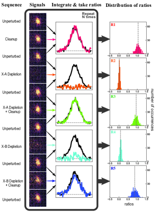
Figure 2: Illustration of the ratio extraction process for the $B^{2}\Sigma^{+}$ ($v^{\prime}=0$) predissociation measurement. We run the stages sequentially with an interlaced reference stage, and collect LIF with an EMCCD. We integrate the images along both axes to obtain the signals, which we then used to calculate ratios. By repeating the entire sequence N times, we collect N sets of five ratios. Here we first show examples of one-shot camera images. We then present the integrated signal along one axis, using colored traces for science stages and black for reference stages (horizontal lines are the baselines). Finally we show the histograms of the five ratios. Vertical dashed lines represent the means of the ratios.

V.2 $B^{2}\Sigma^{+}$ $(v^{\prime}=0)$ predissociation measurement method

To measure the predissociation probability of the $B^{2}\Sigma^{+}$ ($v^{\prime}=0$) state, we need to scatter many photons via $B^{2}\Sigma^{+}$ ($v^{\prime}=0$) and detect population loss that cannot be explained by known effects, predominantly rovibrational losses. To characterize the loss we design several experimental stages, each stage corresponding to a unique configuration of lasers interacting with the molecular beam. We monitor the population of the $v^{\prime\prime}=0$ ground state in the detection region by detecting LIF signals from the $B^{D}_{0-0}$ laser. For this measurement we employ 6 stages. By defining temporally stable parameters that describe the properties of our system, we can express the molecular population distribution at each stage.

For example, in the Unperturbed stage we detect $X(v^{\prime\prime}=0)$ population denoted by $N$. This is the calibration signal used as a reference. In the Cleanup stage we apply the $B^{C}_{0-1}$ laser, and the resulting $X(v^{\prime\prime}=0)$ population is $N+n_{1}N\kappa F_{B00}/\mathcal{F}_{B0}$ where $n_{1}$ is the normalized natural population of $X(v^{\prime\prime}=1)$, $\kappa$ is the cleanup laser efficiency, and $\mathcal{F}_{B_{0}}\equiv F_{B0a}+\sum_{i\neq 1}F_{B0i}$ is the VBR normalization factor. This factor accounts for the discrete probability distribution of decay processes based on the VBRs and $P_{\mathrm{pd}}$. By taking the ratio of the integrated signal of the $X(v^{\prime\prime}=0)$ population from the Cleanup stage with signal from the Unperturbed stage, we get the parametrized ratio $R_{1}=1+n_{1}\kappa F_{B00}/\mathcal{F}_{B0}$. In addition to the Unperturbed and Cleanup stages, we have four more stages in this measurement, resulting in a total of 5 ratios and 5 parameters (including $P_{\mathrm{pd}}$). The details of all the stages, such as the laser configurations and expressions for the normalized signal, are in Table 2 and Appendix C. Thus we acquire 5 equations (measured ratios equal to the parametrized expressions) and 5 variables. We can solve the equations and express $F_{B0a}$ via $R_{i}$s. By precisely measuring $R_{i}$ we can estimate the $B^{2}\Sigma^{+}$ $(v^{\prime}=0)$ predissociation probability.

Purpose	Upstream Laser Config	Downstream Normalized $X^{2}\Sigma^{+}$ $(v^{\prime\prime}=0)$ State Pop	Averaged Signal Ratio
Unperturbed	-	1	-
Cleanup	$B^{C}_{0-1}$	$1+n_{1}\kappa F_{B00}/\mathcal{F}_{B_{0}}$	1.05(2)
X-A Cycling	$A^{I}_{0-0}$	$d_{A}$	0.018(6)
X-A Cycling + Cleanup	$A^{I}_{0-0}+B^{C}_{0-1}$	$d_{A}+[(1-d_{A})F_{A01}/\mathcal{F}_{A_{0}}+n_{1}]\kappa F_{B00}/\mathcal{F}_{B_{0}}$	0.94(2)
X-B Cycling	$B^{I}_{0-0}$	$d_{B}$	0.086(8)
X-B Cycling + Cleanup	$B^{I}_{0-0}+B^{C}_{0-1}$	$d_{B}+[(1-d_{B})F_{B01}/\mathcal{F}_{B_{1}}+n_{1}]\kappa F_{B00}/\mathcal{F}_{B_{0}}$	0.87(2)

Table 2: Experimental stages for $B(v^{\prime}=0)$ state predissociation measurement. In the second column, $M^{{R}}_{v^{\prime}-v^{\prime\prime}}$ denotes the laser information. $M$ is $A$ or $B$, representing the electronic excited state. ${R}$ denotes the region $S$, $I$, or $C$ (see text). The third column contains the normalized ground-state populations using unknown variables and calculated VBRs. The five variables $n_{1}$, $\kappa$, $F_{B0a}$, $d_{A}$ and $d_{B}$ represent $X(v^{\prime\prime}=1)$ state natural population, cleanup efficiency of laser $B^{C}_{1-0}$, $B(v^{\prime}=0)$ state predissociation probability, depletion efficiency of laser $A^{I}_{0-0}$ and depletion efficiency of laser $B^{I}_{0-0}$. We denote the VBR normalization factors as $\mathcal{F}_{A_{0}}\equiv\sum_{i\neq 0}F_{A0i}$, $\mathcal{F}_{B_{0}}\equiv F_{B0a}+\sum_{i\neq 1}F_{B0i}$, and $\mathcal{F}_{B_{1}}\equiv F_{B0a}+\sum_{i\neq 0}F_{B0i}$. Additional information is in Appendix C.

V.3 $B^{2}\Sigma^{+}$ $(v^{\prime}=1)$ predissociation measurement method

For the $B(v^{\prime}=1)$ state, predissociation is also measured within the framework of stages. We implement two different methods, each consisting of multiple laser configurations, to measure the same quantity. In method I we use 6 stages, always monitoring the $X(v^{\prime\prime}=0)$ population downstream using laser $A^{D}_{0-0}$. The aim is to populate $X(v^{\prime\prime}=1)$ via an off-diagonal pumping laser $A^{S}_{1-0}$ and perform optical cycling between $X(v^{\prime\prime}=1)$ and $B(v^{\prime}=1)$. We expect to see an increase of the $X(v^{\prime\prime}=0)$ population as a result of the cycling. We repump the molecules remaining in $X(v^{\prime\prime}=1)$ to $v^{\prime\prime}=0$. The recovered population might be less than expected due to vibrational loss. By ruling out other effects, we attribute the loss to $B(v^{\prime}=1)$ predissociation. The details of the 6 stages are in Table 3.

Method II differs in several ways. We monitor the $X(v^{\prime\prime}=1)$ population instead of $v^{\prime\prime}=0$, accounting for loss to both $v^{\prime\prime}=0$ and $v^{\prime\prime}=2$ with a sufficient signal-to-noise ratio (SNR) using laser $B^{D}_{1-1}$. The 10 stages in this method lead to 9 measured ratios. And the 7 required parameters imply that there are more equations than variables. To find the optimal solution of this over-constrained system, we define a least-squares objective function and use the Levenberg-Marquardt algorithm to search for the local minimum in the parameter space with reasonable initial guesses.

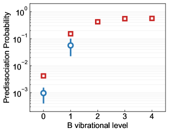
Figure 3: CaH predissociation. Red squares are theoretical results for nonradiative decay rates of different vibrational states of $B^{2}\Sigma^{+}$. Blue circles are experimental results, where error bars represent the 95% confidence interval.

Purpose	Upstream Laser Config	Downstream Normalized $X^{2}\Sigma^{+}$ $(v^{\prime\prime}=0)$ State Pop	Averaged Signal Ratio
Unperturbed	-	1	-
State Prep	$A^{S}_{1-0}$	$1-a$	0.22(2)
Cleanup	$A^{C}_{0-1}$	$1+n_{1}\kappa F_{A00}/\mathcal{F}_{A_{1}}$	1.10(3)
State Prep + Cleanup	$A^{S}_{1-0}+A^{C}_{0-1}$	$1-a+(n_{1}+aF_{A11}/\mathcal{F}_{A_{2}})\kappa F_{A00}/\mathcal{F}_{A_{1}}$	1.01(3)
State Prep + X-B 1-1 Cycling	$A^{S}_{1-0}+B^{I}_{1-1}$	$1-a+(n_{1}+aF_{A11}/\mathcal{F}_{A_{2}})d_{B}F_{B10}/\mathcal{F}_{B_{2}}$	0.39(2)
State Prep + X-B 1-1 Cycling + Cleanup	$A^{S}_{1-0}+B^{I}_{1-1}+A^{C}_{0-1}$	$1-a+(n_{1}+aF_{A11}/\mathcal{F}_{A_{2}})(d_{B}F_{B10}/\mathcal{F}_{B_{2}}$ $+(1-d_{B})\kappa F_{A00}/\mathcal{F}_{A_{1}})$	0.40(2)

Table 3: Method I of $B^{2}\Sigma^{+}$ $(v^{\prime}=1)$ predissociation measurement. Notation is similar to Table 2. In the third column, the variables include $a$, $n_{1}$, $\kappa$, $F_{B1a}$ and $d_{B}$, representing state preparation (from $X(v^{\prime\prime}=0)$ to $X(v^{\prime\prime}=1)$) efficiency, $X(v^{\prime\prime}=1)$ natural population, cleanup efficiency of laser $A^{C}_{0-1}$, $B(v^{\prime}=1)$ predissociation probability and depletion efficiency of laser $B^{I}_{1-1}$. The VBR normalization factors are $\mathcal{F}_{A_{1}}\equiv\sum_{i\neq 1}F_{A0i}$, $\mathcal{F}_{A_{2}}\equiv\sum_{i\neq 0}F_{A1i}$, and $\mathcal{F}_{B_{2}}\equiv F_{B1a}+\sum_{i\neq 1}F_{B1i}$. Additional information is in Appendix C.

Purpose	Upstream Laser Config	Downstream Normalized $X^{2}\Sigma^{+}$ $(v^{\prime\prime}=1)$ State Pop	Avg Ratio
State Prep + Cleanup v0	$A^{S}_{1-0}+A^{C}_{1-0}$	$n_{1}+(a+\kappa_{1}-a\kappa_{1})F_{A11}/\mathcal{F}_{A_{2}}$	-
Unperturbed	-	$n_{1}$	0.13(3)
State Prep	$A^{S}_{1-0}$	$n_{1}+aF_{A11}/\mathcal{F}_{A_{2}}\equiv\mathcal{Z}$	0.89(4)
Cleanup v0	$A^{C}_{1-0}$	$n_{1}+\kappa_{1}F_{A11}/\mathcal{F}_{A_{2}}$	0.93(4)
State Prep + X-A 1-1 Cycling	$A^{S}_{1-0}+A^{I}_{1-1}$	$\mathcal{Z}(1-d_{A})$	0.03(3)
State Prep + X-A 1-1 Cycling + Cleanup v0	$A^{S}_{1-0}+A^{I}_{1-1}+A^{C}_{1-0}$	$\mathcal{Z}(1-d_{A})+(1-a+\mathcal{Z}d_{A}F_{A10}/\mathcal{F}_{A_{3}})\kappa_{1}F_{A11}/\mathcal{F}_{A_{2}}$	0.33(3)
State Prep + X-A 1-1 Cycling + Cleanup v2	$A^{S}_{1-0}+A^{I}_{1-1}+A^{C}_{1-2}$	$\mathcal{Z}(1-d_{A})+(aF_{A12}/\mathcal{F}_{A_{2}}+\mathcal{Z}d_{A}F_{A12}/\mathcal{F}_{A_{3}})\kappa_{2}F_{A11}/\mathcal{F}_{A_{4}}$	0.57(4)
State Prep + X-B 1-1 Cycling	$A^{S}_{1-0}+B^{I}_{1-1}$	$\mathcal{Z}(1-d_{B})$	0.12(3)
State Prep + X-B 1-1 Cycling + Cleanup v0	$A^{S}_{1-0}+B^{I}_{1-1}+A^{C}_{1-0}$	$\mathcal{Z}(1-d_{B})+(1-a+\mathcal{Z}d_{B}F_{B10}/\mathcal{F}_{B_{2}})\kappa_{1}F_{A11}/\mathcal{F}_{A_{2}}$	0.35(3)
State Prep + X-B 1-1 Cycling + Cleanup v2	$A^{S}_{1-0}+B^{I}_{1-1}+A^{C}_{1-2}$	$\mathcal{Z}(1-d_{B})+(aF_{A12}/\mathcal{F}_{A_{2}}+\mathcal{Z}d_{B}F_{B12}/\mathcal{F}_{B_{2}})\kappa_{2}F_{A11}/\mathcal{F}_{A_{4}}$	0.42(3)

Table 4: Method II of $B^{2}\Sigma^{+}$ $(v^{\prime}=1)$ predissociation measurement. In the third column, the 7 variables include $a$, $n_{1}$, $\kappa_{1}$, $\kappa_{2}$, $F_{B1a}$, $d_{A}$ and $d_{B}$, representing state preparation (from $X(v^{\prime\prime}=0)$ to $X(v^{\prime\prime}=1)$) efficiency, $X(v^{\prime\prime}=1)$ natural population, cleanup efficiency of laser $A^{C}_{1-0}$, cleanup efficiency of laser $A^{C}_{1-2}$, $B(v^{\prime}=1)$ predissociation probability, depletion efficiency of laser $A^{I}_{1-1}$ and depletion efficiency of laser $B^{I}_{1-1}$. The VBR normalization factors are $\mathcal{F}_{A_{2}}\equiv\sum_{i\neq 0}F_{A1i}$, $\mathcal{F}_{A_{3}}\equiv\sum_{i\neq 1}F_{A1i}$, $\mathcal{F}_{A_{4}}\equiv\sum_{i\neq 2}F_{A1i}$, and $\mathcal{F}_{B_{2}}\equiv F_{B1a}+\sum_{i\neq 1}F_{B1i}$. Additional information is in Appendix C.

V.4 Predissociation measurement analysis

The yield of our CBGB source exhibits some slow drift. In order to reduce errors due to molecule number fluctuations, we insert a reference stage before and after every other stage within a group when taking data. For example, in the $B(v^{\prime}=0)$ predissociation measurement, data are taken in the following order: Unperturbed $\rightarrow$ Cleanup $\rightarrow$ Unperturbed $\rightarrow$ X-A Cycling $\rightarrow$ Unperturbed … X-B Cycling + Cleanup $\rightarrow$ Unperturbed. The reference stage for $B(v^{\prime}=1)$ method I is Unperturbed, while for method II it is State Prep + Cleanup v0. To calculate the ratios, we divide the signal by the average signal from the calibration shots before and after. The entire group of measurements is repeated multiple times. The averaged ratios can be found in Tables 2, 3, and 4. The values in parentheses denote the $2\sigma$ statistical errors. A graphical representation of the analysis process and histograms of all five ratios can be found in Fig. 2.

With the ratios measured, we use a bootstrap method [45, 46, 47] to derive the mean values and build the confidence intervals of the predissociation probabilities depicted in Fig. 3. This method is particularly useful as it does not require any assumptions about the data such as independence assumptions typically made for standard error calculations. We consider several other analysis methods, such as pairwise bootstrapping and regular error propagation, and the outcomes are all in agreement with each other. Details of the bootstrap method are in Appendix D.

After considering all systematic effects and analyzing statistical errors, we find the predissociation probability for the $B^{2}\Sigma^{+}$ $(v^{\prime}=0)$ state to be $0.00097^{+0.00059}_{-0.00057}$ and for the $B^{2}\Sigma^{+}$ $(v^{\prime}=1)$ state to be $0.056^{+0.044}_{-0.034}$. The reported value for $B(v^{\prime}=1)$ is the average of the two methods (method I yields $0.079^{+0.021}_{-0.017}$ and method II yields $0.033^{+0.013}_{-0.011}$), and the 95% confidence interval is the largest of the two methods combined. These values are consistent with the probabilities calculated in Sec. IV within the order of magnitude. Other potential loss channels are discussed in Appendix A. In addition, to demonstrate the robustness of our measurements to small variations in FCFs, we perform a comparative analysis by utilizing the FCFs obtained in previous theoretical work on CaH [20, 48]. The results consistently produce nonzero predissociation probabilities and are within error bars of each other. The sharp monotonic increase in $P_{\mathrm{pd}}$ seen in Fig. 3 can be understood as a bound molecule quantum tunneling through the $B^{2}\Sigma^{+}$ potential into the $X^{2}\Sigma^{+}$ continuum at the same energy. As the energy of the incident quantum state increases, so does the transmission probability, which is aided by stronger wavefunction overlaps.

	$A^{2}\Pi_{x}$ $(v=0,m_{s}=1/2)$	$A^{2}\Pi_{y}$ $(v=0,m_{s}=1/2)$	$B^{2}\Sigma^{+}$ $(v=0,m_{s}=-1/2)$
$A^{2}\Pi_{x}$ $(v=0,m_{s}=1/2)$	0	-35.5$i$	21.5
$A^{2}\Pi_{y}$ $(v=0,m_{s}=1/2)$	35.5$i$	0	-21.5$i$
$B^{2}\Sigma^{+}$ $(v=0,m_{s}=-1/2)$	21.5	21.5$i$	1400

	$A^{2}\Pi_{x}$ $(v=1,m_{s}=1/2)$	$A^{2}\Pi_{y}$ $(v=1,m_{s}=1/2)$	$B^{2}\Sigma^{+}$ $(v=0,m_{s}=-1/2)$	$B^{2}\Sigma^{+}$ $(v=1,m_{s}=-1/2)$
$A^{2}\Pi_{x}$ $(v=1,m_{s}=1/2)$	0	-35.5$i$	21.5$f$	21.5
$A^{2}\Pi_{y}$ $(v=1,m_{s}=1/2)$	35.5$i$	0	-$(21.5f)i$	-21.5$i$
$B^{2}\Sigma^{+}$ $(v=0,m_{s}=-1/2)$	21.5$f$	$(21.5f)i$	64	0
$B^{2}\Sigma^{+}$ $(v=1,m_{s}=-1/2)$	21.5	21.5$i$	0	1310

Table 5: Spin-orbit matrices accounting for vibrational mixing of the $A$ and $B$ states. The $\Pi_{x}$ and $\Pi_{y}$ basis states split under SOC to produce $\Pi_{1/2}$ and $\Pi_{3/2}$ states. The top matrix is for $A^{2}\Pi$ $(v^{\prime}=0)$ and $B^{2}\Sigma^{+}$ $(v^{\prime}=0)$, while the bottom one is for $A^{2}\Pi$ $(v^{\prime}=1)$, $B^{2}\Sigma^{+}$ $(v^{\prime}=1)$ and $B^{2}\Sigma^{+}$ $(v^{\prime}=0)$. The Franck-Condon factor $f$ is introduced to account for the off-diagonal vibrational wavefunction overlap. The diagonal terms represent the energies of unperturbed states. All values are in cm^-1.

VI $A^{2}\Pi_{1/2}$ Predissociation estimate

The $A^{2}\Pi$ state in CaH does not undergo predissociation via the process described for the $B^{2}\Sigma^{+}$ state. However, spin-orbit coupling can induce mixing between the $A$ and $B$ states, leading to non-vanishing predissociation of the $A^{2}\Pi_{1/2}$ spin-orbit state. For a linear molecule, the $z$-component of total angular momentum, $J_{z}$, is a good quantum number. Therefore the spin-orbit component $A^{2}\Pi_{1/2}$can interact with $B^{2}\Sigma^{+}(J_{z}=1/2)$ due to the same $J_{z}$ value. A similar interaction exists between $A^{2}\Pi_{1/2}$ and $X^{2}\Sigma^{+}(J_{z}=1/2)$ but the energy separation is much larger ($\sim$14,000 cm^-1) compared to that between the $A$ and $B$ states ($\sim$1,400 cm^-1). Higher vibrational states of the $X$ manifold are closer in energy to $A$ but the effective coupling to the states relevant for laser cooling is weaker due to a poor vibrational wavefunction overlap.

We estimate the mixing between the $A(v^{\prime}=0)$ and the $B(v^{\prime}=0)$ states separated by 1400 cm^-1. The spin-orbit parameters are obtained with the Breit-Pauli Hamiltonian at the MRCI level [37] and are given in Table 5. Diagonalization of this Hamiltonian matrix leads to a 0.05% $B(v^{\prime}=0)$ admixture into the $A(v^{\prime}=0)$ state. Similarly, we can compute the mixing between $A(v^{\prime}=1)$, $B(v^{\prime}=0)$, and $B(v^{\prime}=1)$. The coupling between $A(v^{\prime}=1)$ and $B(v^{\prime}=1)$ is expected to be similar to the case of $v^{\prime}=0$ since the energy difference of 1310 cm^-1 is similar to that in the case of $v^{\prime}=0$. However, the $A(v^{\prime}=1)$ and $B(v^{\prime}=0)$ states are only 64 cm^-1 apart, hence even a small FCF can lead to significant mixing. Note that the measured FCF for the $A(v^{\prime}=0)\rightarrow X(v^{\prime\prime}=1)$ transition is 4% (Table 1) and that our calculated $A-B$ bond length difference is smaller than the $X-A$ bond length. We use $f=5$% as an upper limit for the $A(v^{\prime}=1)\rightarrow B(v^{\prime}=0)$ FCF. Diagonalization of the corresponding Hamiltonian matrix in Table 5 yields a 8.4% $B(v^{\prime}=0)$ character for $A(v^{\prime}=1)$. Combining these admixtures with the measured $P_{\mathrm{pd}}$ for $B(v^{\prime}=0,1)$, we estimate that the $A(v^{\prime}=0)$ state very weakly predissociates with a probability of $\sim 5\times 10^{-7}$ and the $A(v^{\prime}=1)$ state with a higher probability of $\sim 3\times 10^{-5}$. The FCF used here is an upper-bound value and therefore the estimated probabilities serve as upper bounds.

VII Controlled Dissociation Pathway

As mentioned in Sec. I, an enticing application of ultracold CaH and other molecules is controlled dissociation into fragments that are not directly laser-coolable, such as H. In order to trap the resulting H atoms, their maximum kinetic energy must be below typical optical trap depths. A magic-wavelength trap for H atoms at 513 nm has a depth of 1.2 kHz per 10 kW/cm² [49]. A practical dipole trap with an intensity of at most $\sim$100 kW/cm² would result in a maximum trap depth of only $\sim 0.5\leavevmode\nobreak\ \mu$K. Since the binding energy of $B^{2}\Sigma^{+}$ $(v^{\prime}=0)$ corresponds to a temperature of $\sim 1,000$ K, the trapping of the fragments relies on the ability to dissociate the molecules as closely as possible to the threshold [26], such as via a stimulated two-photon process [50, 51].

Stimulated Raman adiabatic passage (STIRAP) is a technique that has been successfully employed to generate ground-state bialkali molecules starting from a weakly bound state [52, 53]. Although STIRAP has been predominantly demonstrated for adiabatic population transfers from weakly bound to deeply bound molecular states, the mechanism can be extended to unbound continuum states [54, 55]. A prerequisite for efficient transfer is the identification of an intermediate state that strongly couples to both initial and final states. Additionally, a desirable intermediate state would be connected via readily accessible laser wavelengths to the initial and final states.

Molecular structure calculations give us access to branching ratios and line strengths for a multitude of vibrational levels, some of which have advantages for controlled dissociation. We calculate the dipole transition line strength $S_{v^{\prime}v^{\prime\prime}}$, which is the square of the transition dipole moment $(|\bra{v^{\prime}}\mu\ket{v^{\prime\prime}}|^{2})$, for both $A^{2}\Pi_{1/2}$ $\rightarrow$$X^{2}\Sigma^{+}$ and $B^{2}\Sigma^{+}$ $\rightarrow$$X^{2}\Sigma^{+}$ transitions (Figs. 4(a,b)). The PES for $A$ and $X$ state are similar in shape (Fig. 1(a)) which leads to highly diagonal transition strengths. However, the second minimum in the $B$ state PES leads to strong off-diagonal coupling starting around $v^{\prime}=4$. This feature enables strong coupling of $B(v^{\prime}=4)$ to both $X(v^{\prime\prime}=0)$ and $X(v^{\prime\prime}=15)$ (Fig. 4(c)). Our calculations do not show a significant coupling between the $B(v^{\prime}=4)$ state and the vibrationally excited states of the A manifold. Here we calculate the coupling to the weakest bound state, rather than to the continuum, for two reasons. First, we expect the coupling to the lowest-energy continuum states and to the least-bound state to be similar since their energy difference is only $\sim 500$ cm^-1. Second, we expect the STIRAP process to be more efficient if all three states are bound states. Hence it is worthwhile to consider a transfer to $X(v^{\prime\prime}=15)$ followed by photodissociation [51] or Feshbach dissociation [56].

In Fig. 4(d) we plot the laser wavelengths required to connect $X(v^{\prime\prime}=0)$ as well as the ground-state continuum to the $B$ manifold. We estimate that the “upleg" STIRAP wavelength for $X(v^{\prime\prime}=0)\rightarrow B(v^{\prime}=4)$ is 512.7 nm while the “downleg" wavelength for $B(v^{\prime}=4)\rightarrow X(v^{\prime\prime}=v_{\mathrm{th}})$ is 1744.7 nm. Both these wavelengths are accessible via current technology such as Raman fiber amplifiers and difference-frequency generation (DFG). Thus we expect high-power and narrow-linewidth laser sources to be within reach for STIRAP.

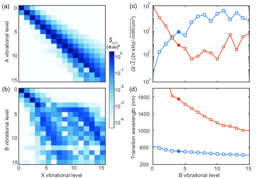
Figure 4: Suggested controlled dissociation pathway for CaH molecules. Line strengths ($S_{v^{\prime}v^{\prime\prime}}$) in atomic units for dipole allowed transitions: (a) $X^{2}\Sigma^{+}$ $(v^{\prime\prime})\rightarrow$$A^{2}\Pi_{1/2}$ $(v^{\prime})$ and (b) $X^{2}\Sigma^{+}$ $(v^{\prime\prime})\rightarrow$$B^{2}\Sigma^{+}$ $(v^{\prime})$. The $A$ state potential is more harmonic as is reflected by the diagonal $S_{v^{\prime}v^{\prime\prime}}$. The $B$ state, however, significantly deviates from the diagonal starting around $v^{\prime}=4$ because of the second potential minimum at $\sim 6$ $a_{0}$ (Fig. 1(a)). Note that $B(v^{\prime}=4)$ has comparable line strengths between $X(v^{\prime\prime}=0)$ and $X(v^{\prime\prime}=15)$. (c) Intensity-normalized Rabi rate ($\Omega/\sqrt{I}=\sqrt{S_{v^{\prime}v^{\prime\prime}}}/\hbar$) for dipole transitions $X(v^{\prime\prime}=0)\rightarrow B(v^{\prime})$ (red squares) and $B(v^{\prime})\rightarrow X(v=15)$ (blue circles). Around $v^{\prime}=4$ (shaded points), the Rabi rates are comparable. (d) Wavelengths in nanometers for optical transitions $X(v^{\prime\prime}=0)\rightarrow B(v^{\prime})$ (blue circles) and $B(v^{\prime})\rightarrow X$(continuum) (red squares). The theoretical energy differences are adjusted by a common offset of 240 cm^-1 to match experimental data for $X(v^{\prime\prime}=0)\rightarrow B(v^{\prime}=0,1,2)$ transitions [57]. The wavelengths corresponding to $v^{\prime}=4$ (shaded points) are 512.7 nm and 1744.7 nm.

VIII Conclusion

Predissociation is a challenge for laser cooling of new molecular species. We have theoretically and experimentally studied it for laser cooling CaH as well as in the context of controlled ultracold dissociation. We find that the lowest-excited electronic state $A^{2}\Pi_{1/2}$ $(v^{\prime}=0)$, which is the workhorse for optical cycling, only weakly predissociates ($P_{\mathrm{pd}}$ $\approx 10^{-6}$) via spin-orbit coupling. The next excited manifold $B^{2}\Sigma^{+}$, crucial for repumping vibrational dark states, has much stronger predissociation by virtue of having the same symmetry as $X^{2}\Sigma^{+}$. We measure $P_{\mathrm{pd}}$ for $B(v^{\prime}=0)$ and $B(v^{\prime}=1)$ states and obtain $\sim 10^{-3}$ and $\sim 6\times 10^{-2}$, respectively. This sharp increase is substantiated by theoretical calculations, and we expect $P_{\mathrm{pd}}$ $\rightarrow 1$ for $v^{\prime}\gtrsim 4$. The results are summarized in Table 6.

To obtain high photon scattering rates, one must repump the $A(v^{\prime}=0)\rightarrow X(v^{\prime\prime}=1)$ vibrational loss channel via the $B(v^{\prime}=0)$ state. Due to predissociation, we find that the optimal laser cooling scheme requires avoiding the $B(v^{\prime}\geq 1)$ states in favor of using the $A$ manifold. On average, every cycling molecule will scatter $\sim 20$ photons $(1/(1-F_{A00}))$ before being lost to $X(v^{\prime\prime}=1)$. Each of these molecules only needs to scatter one photon via $B(v^{\prime}=0)$ to return to cycling, but it will predissociate with a 0.1% probability. Hence we estimate that $\sim 50\%$ of molecules will be lost to predissociation after scattering the requisite $\sim 10^{4}$ photons.

Last, we propose to take advantage of the high predissociation probability for $B(v^{\prime}=4)$ state to engineer a two-photon STIRAP pathway for transferring the molecular population from the ground $X(v^{\prime\prime}=0)$ state to the low-energy continuum $X(v^{\prime\prime}=v_{\mathrm{th}})$. We find that $B(v^{\prime}=4)$ couples strongly to both these $X$ states via optical transitions at wavelengths within accessible laser technologies.

State	Vibrational quantum $(v^{\prime\prime})$	Radiative lifetime (ns)	Radiative decay rate ($A_{R}$, s-1)	Nonradiative decay rate ($A_{\mathrm{NR}}$, s-1)	Predissociation (PD) probability	Experimental PD probability
B	0	52.0	1.924$\times 10^{7}$	8.040$\times 10^{4}$	0.0042	$0.00097_{-0.00057}^{+0.00059}$
	1	54.3	1.842$\times 10^{7}$	3.304$\times 10^{6}$	0.1521	$0.056^{+0.044}_{-0.034}$
	2	58.9	1.698$\times 10^{7}$	1.245$\times 10^{7}$	0.4230	-
	3	78.2	1.278$\times 10^{7}$	1.571$\times 10^{7}$	0.5514	-
	4	59.2	1.688$\times 10^{7}$	2.181$\times 10^{7}$	0.5637	-
	5	83.9	1.193$\times 10^{7}$	5.482$\times 10^{7}$	0.8213	-
	6	84.4	1.185$\times 10^{7}$	5.960$\times 10^{7}$	0.8342	-
A	0	34.3	2.913$\times 10^{7}$	-	-	5$\times 10^{-7}$
	1	34.5	2.902$\times 10^{7}$	-	-	3$\times 10^{-5}$

Table 6: Theoretical and experimental values of predissociation probability for $B^{2}\Sigma^{+}$ and $A^{2}\Pi_{1/2}$. Both radiative ($A_{R}$) and non-radiative ($A_{\mathrm{NR}}$) decay rates are calculated. The radiative lifetime is $\tau\equiv 1/A_{R}$. Predissociation $P_{\mathrm{pd}}$ probability is defined as the ratio of the nonradiative decay rate to the total decay rate $(A_{R}+A_{\mathrm{NR}})$. Measurements of $P_{\mathrm{pd}}$ are only provided for the $B^{2}\Sigma^{+}$ $(v^{\prime}=0)$ and $(v^{\prime}=1)$ states. For the latter, we report the mean of two different measurement methods described in Section V.3. The values given for the $A^{2}\Pi_{1/2}$ $(v^{\prime}=0)$ and $(v^{\prime}=1)$ states are estimated by calculating the spin-orbit mixing between $A$ and $B$ as described in Section VI.

Appendix A Other possible loss channels and their contributions

Other potential loss channels that disrupt optical cycling could lead to overestimating the predissociation probability. The theoretical results are agnostic to such processes. We consider the following processes that may contribute to population loss:

• Off-resonant excitation to the $B^{2}\Sigma^{+}$ $(v^{\prime}=0,N^{\prime}=2)$ state. The nearest parity-allowed transition from $X(v^{\prime\prime}=0,N^{\prime\prime}=1)$ is to $B(v^{\prime}=0,N^{\prime}=2)$ which is 768 GHz away from $B(v^{\prime}=0,N^{\prime}=1)$. The transition linewidth is $\sim 2\pi\times 3$ MHz. Assuming a two-level-like system, the scattering rate is [1]

  $$R_{\mathrm{sc}}=\frac{s\Gamma/2}{1+s+(2\Delta/\Gamma)^{2}}.$$

  In our system, the saturation parameter is $s\lesssim 1,000$, and thus $R_{\mathrm{sc}}\lesssim 2$ s^-1. This rate is low compared to the estimated nonradiative decay rate of $10^{5}$ s^-1, therefore off-resonant excitation should not affect the result.

• External electric fields $\epsilon$ can induce mixing between $B^{2}\Sigma^{+}$ $(v^{\prime}=0,N^{\prime}=0)$ and $N^{\prime}=1$ states (e.g., Ref. [58], Section 8.4.2.1). For the $A^{2}\Pi_{1/2}$ state, the matrix element of the dipole operator $T^{1}_{p}(d)$ in Hund’s case $a$ basis is $-\frac{1}{3}\epsilon d$. For the $B^{2}\Sigma^{+}$ state expressed in Hund’s case $b$ basis, we first project to Hund’s case $a$ basis, then calculate the matrix element to be $-\frac{1}{2}\epsilon d$. The rotational spacing for $B^{2}\Sigma^{+}$ is 250 GHz, while the $\Lambda$-doubling for $A^{2}\Pi_{1/2}$ is 26 GHz [57]. The effective decay rate is given by

  $$\frac{1}{\tau^{N=0,2}}=R_{\mathrm{sc}}\frac{(d\epsilon/2)^{2}}{4\omega^{2}+\Gamma^{2}/4},$$

  where for the $A$ and $B$ states respectively, the values are $d$ = 2.57 D and 3.1 D, $\omega=2\pi\times 13$ GHz and $2\pi\times 125$ GHz, and $\Gamma=2\pi\times 5$ MHz and $2\pi\times 3$ MHz. We assume $R_{\mathrm{sc}}\approx 1$ MHz. Since we electrically ground the entire vacuum chamber, the electric field amplitude inside the chamber should be $<100$ V$/$m. We find that the possible remixing rate is $6.2\times 10^{-4}$ s^-1 for $A^{2}\Pi_{1/2}$ and $9.7\times 10^{-6}$ s^-1 for $B^{2}\Sigma^{+}$. These numbers are several orders of magnitude smaller than nonradiative decay rates and should have a negligible effect.

• Photon scattering along the molecular beam can cause acceleration or deceleration and affect signal strength. In the interaction region we scatter $<100$ photons per molecule. The laser beams are reflected in a zig-zag pattern, i.e. the incidence is not perfectly perpendicular and there is a projection on the beam propagation direction. The angle is estimated to be $\arctan(1/15)\approx 4^{\circ}$. Hence less than 10 photons worth of momentum is added to the molecular beam, and that would only yield a 15 cm$/$s velocity change. The beam velocity is $\sim 200$ m$/$s, implying that the effect on the signal is at the $8\times 10^{-4}$ level which negligible.

• We consider off-diagonal vibrational loss due to spin-orbit mixing. As discussed in Sec. VI, the $B^{2}\Sigma^{+}$ $(v^{\prime}=0)$ state mixes with the $A^{2}\Pi_{1/2}$ $(v^{\prime}=1)$ state at the 0.06% level. This implies that population from $B(v^{\prime}=0)$ can decay to $X(v^{\prime\prime}=1)$ via $A(v^{\prime}=1)$ at a rate of $6\times 10^{-4}\times F_{A10}\approx 5\times 10^{-4}$. This value is 40 times smaller than the FCF for the $B(v^{\prime}=0)\rightarrow X(v^{\prime\prime}=1)$ decay ($1.92\times 10^{-2}$) and hence is a negligible correction to our model. A similar argument holds for off-diagonal vibrational loss induced by spin-orbit mixing of the $B(v^{\prime}=1)$ state with either $A(v^{\prime}=0)$ or $A(v^{\prime}=2)$.

Appendix B Laser parameters and spectroscopy of transitions used in this work

Here we describe the lasers used in the experiment, and the transition frequencies. All laser beams pass through an electro-optic modulator (EOM) to generate the sidebands needed to address HFS.

• In the state preparation region, the $A^{S}_{1-0}$ light (637 nm) is generated from two sets of injection-locked amplifiers (ILAs) to address the spin-rotation states, with 95 mW of power.

• In the interaction region, multiple lasers are applied. $A^{I}_{0-0}$ (695 nm) or $A^{I}_{1-1}$ (693 nm) light is derived from two ILAs that provide 60 mW in total. $B^{I}_{0-0}$ (635 nm) or $B^{I}_{1-1}$ (636 nm) is from two external-cavity diode lasers (ECDLs) with 52 mW in total.

• In the cleanup region, $B^{C}_{0-1}$ (690 nm) is from two sets of ILAs with 90 mW of power, $A^{C}_{1-0}$ (637 nm) is from two sets of ILAs with 88 mW, and $A^{C}_{1-2}$ (758 nm) or $A^{C}_{0-1}$ (762 nm) is from a SolsTiS continuous-wave Ti:sapphire laser, with 93 mW and a 1 GHz EOM to address the spin-rotation states.

• In the detection region, $B^{D}_{0-0}$ (635 nm) is from two ECDLs with 60 mW of power, $A^{D}_{0-0}$ (695 nm) or $A^{D}_{1-1}$ (693 nm) is from two ILAs with 96 mW of power.

The frequencies of all the transitions that we used are in Table 7. All frequencies are measured transversely to the molecular beam, with $\leq$ 10 MHz statistical uncertainties and $\leq$ 60 MHz systematic uncertainties from the wavemeter. The HFS in the ground states is clearly resolved in all spectra, while the HFS in the excited states is not resolved. Our measurements are consistent with previous work [57].

Ground	$v^{\prime\prime}$	$N^{\prime\prime}$	$J^{\prime\prime}$	$F^{\prime\prime}$	Excited	$v^{\prime}$	$N^{\prime}$	$J^{\prime}$	Frequency (THz)
X	0	1	3/2	2	A	0	-	1/2	431.274552
				1					431.274653
			1/2	1					431.276565
				0					431.276512
X	0	1	3/2	2	B	0	0	1/2	472.026689
				1					472.026790
			1/2	1					472.028702
				0					472.028649
X	1	1	3/2	2	A	1	-	1/2	432.342011
				1					432.342120
			1/2	1					432.343958
				0					432.343902
X	1	1	3/2	2	B	1	0	1/2	471.557078
				1					471.557178
			1/2	1					471.559025
				0					471.558969
X	0	1	3/2	2	A	1	-	1/2	470.113870
				1					470.113971
			1/2	1					470.115873
				0					470.115819
X	2	1	3/2	2	A	1	-	1/2	395.717108
				1					395.717218
			1/2	1					395.718978
				0					395.718928
X	1	1	3/2	2	B	0	0	1/2	434.254840
				1					434.254949
			1/2	1					434.256787
				0					434.256731
X	1	1	3/2	2	A	0	-	1/2	393.502723
				1					393.502832
			1/2	1					393.504670
				0					393.504614

Table 7: Frequencies of all transitions used in the experiment. The $A^{2}\Pi_{1/2}$ and $B^{2}\Sigma^{+}$ states have unresolved hyperfine splittings. The uncertainties are 10 MHz statistical and 60 MHz systematic due to the wavemeter.

Appendix C Details of measurement stages

The general principle for designing measurement stages is to have at least as many independent equations as parameters, which includes the $B$ state predissociation probability. If the number of equations and parameters are equal, as in the cases of $B(v^{\prime}=0)$ and $B(v^{\prime}=1)$ using method I, we can directly express $P_{\mathrm{pd}}$ using the measured ratios. Other parameters will also be determined and analyzed, to serve as consistency checks. When there are more equations than parameters, we define a cost function to minimize the differences between the left- and right-hand sides of all equations (Appendix D). Here we present a detailed explanation of how the stages are used for predissociation probability measurements. We first discuss the simplest $B^{2}\Sigma^{+}$ $(v^{\prime}=0)$ measurement, where the stages include the following:

• Unperturbed. Only the $X(v^{\prime\prime}=0)\rightarrow B(v^{\prime}=0)$ detection lasers are turned on. This stage serves as molecule number calibration. By taking ratios of other stages to this stage, we can eliminate molecule number $N$ from the expressions.

• Cleanup. $B^{C}_{0-1}$ vibrational repumpers are turned on. This stage helps to estimate the $X(v^{\prime\prime}=1)$ natural population.

• X-A Cycling. $A^{I}_{0-0}$ cycling lasers are turned on. This stage can be used to estimate the vibrational population distribution after $X-A$ cycling, and measure the depletion efficiency.

• X-A Cycling + Cleanup. $A^{I}_{0-0}$ cycling lasers and $B^{C}_{0-1}$ repumps are turned on. This stage helps to measure the repump efficiency, given the $X(v^{\prime\prime}=1)$ natural population.

• X-B Cycling. $B^{I}_{0-0}$ cycling lasers are turned on. This stage helps to measure the vibrational population distribution after $X-B$ cycling.

• X-B Cycling + Cleanup. $B^{I}_{0-0}$ cycling lasers and $B^{C}_{0-1}$ repumpers are turned on. Combined with previous stages, this helps to measure the $B^{2}\Sigma^{+}$ state predissociation probability.

To understand the stages better, let us take an example when $N$ ground-state molecules interact with the $X(v^{\prime\prime}=0)\rightarrow A(v^{\prime}=0)$ laser. After optical cycling, the downstream ground-state population decreases to $d_{A}N$ (where $d_{A}<1$ and is measurable simply by taking the ratios of signals). In this process, we describe the depletion efficiency as $1-d_{A}$. We can also describe how $d_{A}$ is distributed among the different vibrational levels of $X^{2}\Sigma^{+}$ using the known VBRs. For example, the population in $X(v^{\prime\prime}=1)$ is $N(1-d_{A})F_{A01}/\mathcal{F}_{A0}+n_{1}N$, where $F_{A01}$, $\mathcal{F}_{A0}$ and $n_{1}$ represent the VBR for $A(v^{\prime}=0)\rightarrow X(v^{\prime\prime}=1)$, the sum of VBRs for $A(v^{\prime}=0)\rightarrow X(v^{\prime\prime}=1,2,3...)$, and normalized $X(v^{\prime\prime}=1)$ natural population, because when a molecule is excited to $B(v^{\prime}=0)$ it eventually decays to a vibrational level or breaks apart. This process follows a discrete probability distribution based on the VBRs and $P_{\mathrm{pd}}$. In the case discussed above, $(1-d_{A})N$ molecules leave $B(v^{\prime}=0)$, and, based on the law of large numbers, we expect the $X(v^{\prime\prime}=1)$ population to become $N(1-d_{A})F_{A01}/\mathcal{F}_{A0}$.

Note that our description relies on population transfer $(1-d_{A})$ rather than the number of scattered photons. In addition, the measurement protocol does not rely on the lasers having good overlap with the molecular beam or with each other, because as long as molecules share the same spatial and velocity distributions shot to shot, the parameters (e.g., cleanup efficiency) remain constant.

Here we briefly introduce the stages in method I of the $B^{2}\Sigma^{+}$ $(v^{\prime}=1)$ $P_{\mathrm{pd}}$ measurement:

• Unperturbed. We always monitor the $X(v^{\prime\prime}=0)$ population, which serves as calibration.

• Cleanup. With an $A^{C}_{0-1}$ laser, we pump the natural population in $X(v^{\prime\prime}=1)$ to $X(v^{\prime\prime}=0)$ to check cleanup efficiency.

• State Prep. With an $A^{S}_{1-0}$ laser, we pump the natural population in $X(v^{\prime\prime}=0)$ to $X(v^{\prime\prime}=1)$ to check state preparation efficiency. Only after efficiently pumping molecules to $X(v^{\prime\prime}=1)$ can we perform high-SNR optical cycling on $X(v^{\prime\prime}=1)\rightarrow B(v^{\prime}=1)$. Otherwise, the predissociation loss is too low to measure.

• State Prep + Cleanup. We first populate $X(v^{\prime\prime}=1)$ with $A^{S}_{1-0}$ laser, then move the $X(v^{\prime\prime}=1)$ population back to $X(v^{\prime\prime}=0)$. The signal size should be comparable to the unperturbed case. This step helps to measure $\kappa$, $a$ and $n_{1}$, which are cleanup efficiency, state preparation efficiency and $X(v^{\prime\prime}=1)$ natural population.

• State Prep + X-B 1-1 Cycling. With most molecules in the $X(v^{\prime\prime}=1)$ state, we can perform optical cycling via $B(v^{\prime}=1)$. We expect a signal increment compared to State Prep due to optical cycling and a redistribution of population based on VBR and $P_{\mathrm{pd}}$.

• State Prep + X-B 1-1 Cycling + Cleanup. By cleaning up the population in $X(v^{\prime\prime}=1)$, we measure the molecules left in $X(v^{\prime\prime}=1)$ after optical cycling. Combined with previous stages, this provides 5 equations and 5 variables including $P_{\mathrm{pd}}$.

Method II is designed as follows. We first perform state preparation to populate the $X(v^{\prime\prime}=1)$ state, similar to method I. By individually repumping the population that leaks to $X(v^{\prime\prime}=0)$ and $X(v^{\prime\prime}=2)$ we get a measure of unwanted loss. This also serves as a comparison of $A^{2}\Pi_{1/2}$ and $B^{2}\Sigma^{+}$ states in terms of the loss distribution. The 10 stages are detailed in Table 4. The fact that method II accounts for losses to both $X(v^{\prime\prime}=0)$ and $X(v^{\prime\prime}=2)$ has advantages and disadvantages On the one hand, method II provides an additional confidence check, with more equations than variables. Our approach to solving the over-constrained equation sets is in Appendix D. On the other hand, the method relies on detection using the $X(v^{\prime\prime}=1)$ state, which leads to lower signals and higher drift sensitivity than detecting on $X(v^{\prime\prime}=0)$. Hence the SNR for method II is not significantly higher than for method I.

Measuring the predissociation probability for $B^{2}\Sigma^{+}$ $(v^{\prime}=2)$ and higher vibrational levels would require pumping the population to $X^{2}\Sigma^{+}$ $(v^{\prime\prime}=2)$ and higher and performing optical cycling there, with repumping to recover the population, and monitoring unexplained loss. However, due to practical limitations in available space and number of lasers, as well as the increased complexity of the required stages, we did not pursue these measurements.

Table 8 contains stage details for the three types of measurement described above.

Purpose	Laser Config	$X^{2}\Sigma^{+}$ $(v^{\prime\prime}=0)$ State Pop Normalized	$X^{2}\Sigma^{+}$ $(v^{\prime\prime}=1)$ State Pop Normalized	$X^{2}\Sigma^{+}$ $(v^{\prime\prime}=2)$ State Pop Normalized
$v^{\prime}=0$ experiment
Unperturbed	-	1	$n_{1}$	$\approx 0$
Cleanup	$B^{C}_{0-1}$	$1+n_{1}\kappa F_{B00}/\mathcal{F}_{B_{0}}$	$n_{1}(1-\kappa)$	$n_{1}\kappa F_{B02}/\mathcal{F}_{B_{0}}$
X-A Cycling	$A^{I}_{0-0}$	$d_{A}$	$(1-d_{A})F_{A01}/\mathcal{F}_{A_{0}}+n_{1}$	$(1-d_{A})F_{A02}/\mathcal{F}_{A_{0}}$
X-A Cycling + Cleanup	$A^{I}_{0-0}+B^{C}_{0-1}$	$d_{A}+[(1-d_{A})F_{A01}/\mathcal{F}_{A_{0}}+n_{1}]\kappa F_{B00}/\mathcal{F}_{B_{0}}$	$[(1-d_{A})F_{A01}/\mathcal{F}_{A_{0}}+n_{1}](1-\kappa)$	$[(1-d_{A})F_{A01}/\mathcal{F}_{A_{0}}+n_{1}]\kappa F_{B02}/\mathcal{F}_{B_{0}}+(1-d_{A})F_{A02}/\mathcal{F}_{A_{0}}$
X-B Cycling	$B^{I}_{0-0}$	$d_{B}$	$(1-d_{B})F_{B01}/\mathcal{F}_{B_{1}}+n_{1}$	$(1-d_{B})F_{B02}/\mathcal{F}_{B_{1}}$
X-B Cycling + Cleanup	$B^{I}_{0-0}+B^{C}_{0-1}$	$d_{B}+[(1-d_{B})F_{B01}/\mathcal{F}_{B_{1}}+n_{1}]\kappa F_{B00}/\mathcal{F}_{B_{0}}$	$[(1-d_{B})F_{B01}/\mathcal{F}_{B_{1}}+n_{1}](1-\kappa)$	$[(1-d_{B})F_{B01}/\mathcal{F}_{B_{1}}+n_{1}]\kappa F_{B02}/\mathcal{F}_{B_{0}}+(1-d_{B})F_{B02}/\mathcal{F}_{B_{1}}$
$v^{\prime}=1$ experiment, method I
Unperturbed	-	$1$	$n_{1}$	$\approx 0$
State Prep	$A^{S}_{1-0}$	$1-a$	$n_{1}+aF_{A11}/\mathcal{F}_{A_{2}}$	$aF_{A12}/\mathcal{F}_{A_{2}}$
Cleanup	$A^{C}_{0-1}$	$1+n_{1}\kappa F_{A00}/\mathcal{F}_{A_{1}}$	$n_{1}(1-\kappa)$	$n_{1}\kappa F_{A02}/\mathcal{F}_{A_{1}}$
State Prep + Cleanup	$A^{S}_{1-0}+A^{C}_{0-1}$	$1-a+(n_{1}+aF_{A11}/\mathcal{F}_{A_{2}})\kappa F_{A00}/\mathcal{F}_{A_{1}}$	$(n_{1}+aF_{A11}/\mathcal{F}_{A_{2}})(1-\kappa)$	$aF_{A12}/\mathcal{F}_{A_{2}}+(n_{1}+aF_{A11}/\mathcal{F}_{A_{2}})\kappa F_{A02}/\mathcal{F}_{A_{1}}$
State Prep + X-B 1-1 Cycling	$A^{S}_{1-0}+B^{I}_{1-1}$	$1-a+(n_{1}+aF_{A11}/\mathcal{F}_{A_{2}})d_{B}F_{B10}/\mathcal{F}_{B_{2}}$	$(n_{1}+aF_{A11}/\mathcal{F}_{A_{2}})(1-d_{B})$	$aF_{A12}/\mathcal{F}_{A_{2}}+(n_{1}+aF_{A11}/\mathcal{F}_{A_{2}})d_{B}F_{A02}/\mathcal{F}_{A_{1}}$
State Prep + X-B 1-1 Cycling + Cleanup	$A^{S}_{1-0}+B^{I}_{1-1}+A^{C}_{0-1}$	$1-a+(n_{1}+aF_{A11}/\mathcal{F}_{A_{2}})[d_{B}F_{B10}/\mathcal{F}_{B_{2}}$ $+(1-d_{B})\kappa F_{A00}/\mathcal{F}_{A_{1}}]$	$(n_{1}+aF_{A11}/\mathcal{F}_{A_{2}})(1-\kappa)(1-d_{B})$	$aF_{A12}/\mathcal{F}_{A_{2}}+(n_{1}+aF_{A11}/\mathcal{F}_{A_{2}})[d_{B}F_{B12}/\mathcal{F}_{B_{2}}$ $+(1-d_{B})\kappa F_{A02}/\mathcal{F}_{A_{1}}]$
$v^{\prime}=1$ experiment, method II
State Prep + Cleanup v0	$A^{S}_{1-0}+A^{C}_{1-0}$	$(1-a)(1-\kappa_{1})$	$n_{1}+(a+\kappa_{1}-a\kappa_{1})F_{A11}/\mathcal{F}_{A_{2}}$	$(a+\kappa_{1}-a\kappa_{1})F_{A12}/\mathcal{F}_{A_{2}}$
Unperturbed	-	$1$	$n_{1}$	$\approx 0$
State Prep	$A^{S}_{1-0}$	$1-a$	$n_{1}+aF_{A11}/\mathcal{F}_{A_{2}}\equiv\mathcal{Z}$	$aF_{A12}/\mathcal{F}_{A_{2}}$
Cleanup v0	$A^{C}_{1-0}$	$1-\kappa_{1}$	$n_{1}+\kappa_{1}F_{A11}/\mathcal{F}_{A_{2}}$	$\kappa_{1}F_{A12}/\mathcal{F}_{A_{2}}$
State Prep + X-A 1-1 Cycling	$A^{S}_{1-0}+A^{I}_{1-1}$	$1-a+\mathcal{Z}d_{A}F_{A10}/\mathcal{F}_{A_{3}}$	$\mathcal{Z}(1-d_{A})$	$aF_{A12}/\mathcal{F}_{A_{2}}+\mathcal{Z}d_{A}F_{A12}/\mathcal{F}_{A_{3}}$
State Prep + X-A 1-1 Cycling + Cleanup v0	$A^{S}_{1-0}+A^{I}_{1-1}+A^{C}_{1-0}$	$(1-a+\mathcal{Z}d_{A}F_{A10}/\mathcal{F}_{A_{3}})(1-\kappa_{1})$	$\mathcal{Z}(1-d_{A})+(1-a+\mathcal{Z}d_{A}F_{A10}/\mathcal{F}_{A_{3}})$ $\kappa_{1}F_{A11}/\mathcal{F}_{A_{2}}$	$aF_{A12}/\mathcal{F}_{A_{2}}+\mathcal{Z}d_{A}F_{A12}/\mathcal{F}_{A_{3}}$ $+(1-a+\mathcal{Z}d_{A}F_{A10}/\mathcal{F}_{A_{3}})\kappa_{1}F_{A12}/\mathcal{F}_{A_{2}}$
State Prep + X-A 1-1 Cycling + Cleanup v2	$A^{S}_{1-0}+A^{I}_{1-1}+A^{C}_{1-2}$	$1-a+\mathcal{Z}d_{A}F_{A10}/\mathcal{F}_{A_{3}}+(aF_{A12}/\mathcal{F}_{A_{2}}$ $+\mathcal{Z}d_{A}F_{A12}/\mathcal{F}_{A_{3}})\kappa_{2}F_{A10}/\mathcal{F}_{A_{4}}$	$\mathcal{Z}(1-d_{A})+(aF_{A12}/\mathcal{F}_{A_{2}}$ $+\mathcal{Z}d_{A}F_{A12}/\mathcal{F}_{A_{3}})\kappa_{2}F_{A11}/\mathcal{F}_{A_{4}}$	$(aF_{A12}/\mathcal{F}_{A_{2}}+\mathcal{Z}d_{A}F_{A12}/\mathcal{F}_{A_{3}})(1-\kappa_{2})$
State Prep + X-B 1-1 Cycling	$A^{S}_{1-0}+B^{I}_{1-1}$	$1-a+\mathcal{Z}d_{B}F_{B10}/\mathcal{F}_{B_{2}}$	$\mathcal{Z}(1-d_{B})$	$aF_{A12}/\mathcal{F}_{A_{2}}+\mathcal{Z}d_{A}F_{B12}/\mathcal{F}_{B_{2}}$
State Prep + X-B 1-1 Cycling + Cleanup v0	$A^{S}_{1-0}+B^{I}_{1-1}+A^{C}_{1-0}$	$(1-a+\mathcal{Z}d_{B}F_{B10}/\mathcal{F}_{B_{2}})(1-\kappa_{1})$	$\mathcal{Z}(1-d_{B})+(1-a+\mathcal{Z}d_{B}F_{B10}/\mathcal{F}_{B_{2}})$ $\kappa_{1}F_{A11}/\mathcal{F}_{A_{2}}$	$aF_{A12}/\mathcal{F}_{A_{2}}+\mathcal{Z}d_{B}F_{B12}/\mathcal{F}_{B_{2}}$ $+(1-a+\mathcal{Z}d_{B}F_{B10}/\mathcal{F}_{B_{2}})\kappa_{1}F_{A12}/\mathcal{F}_{A_{2}}$
State Prep + X-B 1-1 Cycling + Cleanup v2	$A^{S}_{1-0}+B^{I}_{1-1}+A^{C}_{1-2}$	$1-a+\mathcal{Z}d_{B}F_{B10}/\mathcal{F}_{B_{2}}+(aF_{A12}/\mathcal{F}_{A_{2}}$ $+\mathcal{Z}d_{B}F_{B12}/\mathcal{F}_{B_{2}})\kappa_{2}F_{A10}/\mathcal{F}_{A_{4}}$	$\mathcal{Z}(1-d_{B})+(aF_{A12}/\mathcal{F}_{A_{2}}$ $+\mathcal{Z}d_{B}F_{B12}/\mathcal{F}_{B_{2}})\kappa_{2}F_{A11}/\mathcal{F}_{A_{4}}$	$(aF_{A12}/\mathcal{F}_{A_{2}}+\mathcal{Z}d_{B}F_{B12}/\mathcal{F}_{B_{2}})(1-\kappa_{2})$

Table 8: Complete stage information for the $B^{2}\Sigma^{+}$ state predissociation measurement (also summarized in Tables 2, 3, and 4). For $B(v^{\prime}=0)$ we use 5 variables: $n_{1}$, $\kappa$, $F_{B0a}$, $d_{A}$, and $d_{B}$, representing $X(v^{\prime\prime}=1)$ natural population, cleanup efficiency of laser $B^{C}_{1-0}$, the $B(v^{\prime}=0)$ state predissociation probability, depletion efficiency of laser $A^{I}_{0-0}$, and depletion efficiency of laser $B^{I}_{0-0}$. For $B(v^{\prime}=1)$ method I, the 5 variables used are $a$, $n_{1}$, $\kappa$, $F_{B1a}$, and $d_{B}$, representing state preparation (from $X(v^{\prime\prime}=0)$ to $X(v^{\prime\prime}=1)$) efficiency, $X(v^{\prime\prime}=1)$ natural population, cleanup efficiency of laser $A^{C}_{1-0}$, the $B(v^{\prime}=1)$ state predissociation probability, and depletion efficiency of laser $B^{I}_{1-1}$. For $B(v^{\prime}=1)$ method II, the 7 variables are $a$, $n_{1}$, $\kappa_{1}$, $\kappa_{2}$, $F_{B1a}$, $d_{A}$, and $d_{B}$, representing state preparation (from $X(v^{\prime\prime}=0)$ to $X(v^{\prime\prime}=1)$) efficiency, $X(v^{\prime\prime}=1)$ natural population, cleanup efficiency of laser $A^{C}_{1-0}$, cleanup efficiency of laser $A^{C}_{1-2}$, the $B(v^{\prime}=1)$ state predissociation probability, depletion efficiency of laser $A^{I}_{1-1}$, and depletion efficiency of laser $B^{I}_{1-1}$. We denote the VBR normalization factors as $\mathcal{F}_{A_{0}}\equiv\sum_{i\neq 0}F_{A0i}$, $\mathcal{F}_{A_{1}}\equiv\sum_{i\neq 1}F_{A0i}$, $\mathcal{F}_{A_{2}}\equiv\sum_{i\neq 0}F_{A1i}$, $\mathcal{F}_{A_{3}}\equiv\sum_{i\neq 1}F_{A1i}$, $\mathcal{F}_{A_{4}}\equiv\sum_{i\neq 2}F_{A1i}$, $\mathcal{F}_{B_{0}}\equiv F_{B0a}+\sum_{i\neq 1}F_{B0i}$, $\mathcal{F}_{B_{1}}\equiv F_{B0a}+\sum_{i\neq 0}F_{B0i}$, and $\mathcal{F}_{B_{2}}\equiv F_{B1a}+\sum_{i\neq 1}F_{B1i}$.

Appendix D Bootstrap method used in the predissociation data analysis

Bootstrapping is a statistical technique that involves generating multiple samples from a dataset by sampling with replacement [45]. It is a useful tool for constructing confidence intervals for a population parameter, $-$ in this case, the expectation values of predissociation probabilities.

A key benefit of bootstrapping is that it allows one to make inferences about a population based on a sample, without making any assumptions about the underlying distribution of the population. Given the complexity of the functional form of predissociation probability with respect to experimentally measured ratios, utilizing a bootstrap method helps to avoid assuming a normal distribution when determining the confidence interval of predissociation probabilities.

One way to use such a method on a set of data $d$ with size $n$ is to use the array of $d$ data points to generate $n$ “bootstrapped” samples by sampling with replacement. We can then compute a statistic of interest, such as the mean, from the $n$ bootstrapped samples, and save it to a new array. We repeatedly generate $n$ bootstrapped samples, calculate the mean, and save it to the storage array. The resulting distribution of the statistic can then be used to make inferences about the population.

Let us consider the $B(v^{\prime}=0)$ predissociation probability as an example. The experimental procedure to acquire ratios is shown in Fig. 2 and explained in Sec. V.4. All the ratios ($r_{1},\;r_{2},\;r_{3},\;r_{4},\;r_{5}$) are expressed using the variables in Table 2, including $n_{1}$, $\kappa$, $F_{B0a}$, $d_{A}$ and $d_{B}$. Five equations can be explicitly written as

$$\begin{split}r_{1}&=1+n_{1}\kappa F_{B00}/\mathcal{F}_{B_{0}},\\ r_{2}&=d_{A},\\ r_{3}&=d_{A}+[(1-d_{A})F_{A01}/\mathcal{F}_{A_{0}}+n_{1}]\kappa F_{B00}/\mathcal{F}_{B_{0}},\\ r_{4}&=d_{B},\\ r_{5}&=d_{B}+[(1-d_{B})F_{B01}/\mathcal{F}_{B_{1}}+n_{1}]\kappa F_{B00}/\mathcal{F}_{B_{0}}.\end{split}$$ (1)

By solving these 5 equations for 5 variables, we can express $F_{B0a}$ as a function of $r_{i}$ ($i\in\{1,2,3,4,5\}$) with known VBRs. Therefore, we obtain a function $f_{B0a}$ that takes in $r_{i}$ ($i\in\{1,2,3,4,5\}$) and outputs predissociation probability $F_{B0a}$. Here we describe the procedure of performing bootstrap analysis on the data, where the data consists of $n\approx 200$ sets of ratios $\{r_{1},r_{2},r_{3},r_{4},r_{5}\}$, with $r_{i}$ ($i\in\{1,2,3,4,5\}$) being an array of length $n$:

1. Randomly sample $n$ elements from the original $r_{1}$ array with replacement, i.e., elements from the original $r_{1}$ can appear more than once in the new array $r_{1}^{\mathrm{bt}}$. This step mimics the situation where the same measurement is performed again. We carry out independent random sampling with replacement for $r_{2}$, $r_{3}$, $r_{4}$, and $r_{5}$ as well, and obtain $r_{i}^{\mathrm{bt}}$ ($i\in\{1,2,3,4,5\}$) arrays.

2. Calculate the mean of the newly generated $r_{i}^{\mathrm{bt}}$ arrays individually, which can be denoted as $\overline{r_{i}^{\mathrm{bt}}}$. We can feed these $\overline{r_{i}^{\mathrm{bt}}}$s to the function $f_{B0a}$ and store the output in an array $F$.

3. Repeat steps 1 and 2 for $\sim 10^{6}$ times, until the statistical properties such as mean and standard deviation of the normalized distribution of array $F$ converge.

4. Analyze the distribution of $F$. For the expectation value, we use the mean of array $F$. To determine the 95% confidence interval, we take the 2.5% quantile from the distribution of $F$ as the lower bound, and the 97.5% quantile as the upper bound.

The data analysis for $B(v^{\prime}=1)$ method I is almost identical to that for $B(v^{\prime}=0)$. The bootstrap procedures are the same, and the analysis code can be found online.

The data analysis for $B(v^{\prime}=1)$ method II is slightly different from the previous two cases. We no longer have a deterministic function of $F_{B1a}$ because there are 9 equations with 7 variables. To solve this over-constrained system, we perform a least square fit. We write down the 9 equations with all the terms on the right hand side and zeros on the left hand side. Then we define the cost function as the sum of squares of all the right hand sides of the equations, and use the Levenberg-Marquardt algorithm to search for the local minimum with a reasonable initial guess.

Appendix E Theoretical details

The following three-state Hamiltonian (for the $X^{2}\Sigma^{+}$, $B^{2}\Sigma^{+}$ and $D^{2}\Sigma^{+}$ electronic states) is diagonalized to obtain wavefunctions, FCFs, and predissociation estimates:

$$\sum^{3}_{j}H_{j}=\sum_{I}\frac{(\hat{p}^{I}+A^{I}_{ij}(r))^{2}}{2\mu}\phi_{j}(r)+V_{j}(r)\phi_{j}(r).$$ (2)

The first term is the kinetic energy operator, in which $\hat{p}$ is the standard momentum operator, expressed on a grid via the Colbert-Miller derivative. We represent the momentum operator in position space so that we can incorporate the nonadiabatic coupling term directly. This term is computed in the position representation, $A_{ij}(r)=\braket{\Psi_{i}}{\hat{p}\Psi_{j}}$. We obtain $\braket{\Psi{i}}{\frac{\partial}{\partial r}\Psi_{j}}$ from a $dr=0.001a_{0}$ potential energy surface scan via Molpro electronic structure calculations, and interpolate this onto a spline to represent $A_{ij}(r)$. The reduced mass of CaH is $\mu$. Finally, $V(r)$ is obtained from the $dr=0.001a_{0}$ scan via the MRCI+Q Davidson energies and interpolated onto a spline before being incorporated into the Hamiltonian.

At $r_{0}=8$ a.u., an optical potential of the form $-iV(r-r_{0})^{2}/w^{2}$ is added only to the $X^{2}\Sigma^{+}$ state’s $V(r)$ at the PES asymptote with each grid-point to simulate the continuum and create a flux equation. Specifically, the optical absorbing potential must have a width $w$ and depth $V$ which guarantees complete wavepacket absorption and ensures the potential is smooth so that hardly any reflection takes place before the wavepacket enters the potential [44]. The absorber width is chosen to be $w=8\leavevmode\nobreak\ a_{0}$, much larger than the typical de Broglie wavelength of $\sim 0.2\leavevmode\nobreak\ a_{0}$. We choose a depth as the typical energy of the wavepacket, or 0.2 a.u. ($4.4\times 10^{4}$ cm^-1). The Hamiltonian is then diagonalized. The optical potential enforces imaginary eigenvalues that are directly related to nonradiative loss rates, which are then compared to the radiative rates calculated from the MRCI-computed transition dipole moments to obtain a predissociation probability.

For spin-orbit coupling, the active space for $X^{2}\Sigma^{+}$, $A^{2}\Pi_{1/2}$ and $B^{2}\Sigma^{+}$ states must be the same, therefore a compromise is chosen to optimize the $X^{2}\Sigma^{+}$ and $B^{2}\Sigma^{+}$ FCFs over the $A^{2}\Pi_{1/2}$. Interestingly, we note that using our basis set and active space but shifting the $A^{2}\Pi_{1/2}$ potential energy surface can produce FCFs that are equivalent to experimentally measured values, as shown in Table 9. This is because static electron correlation has converged, but important dynamic correlation is missing. This depends on the original orbital active space from CASSCF which then affects the MRCI equilibrium bond length.

Transition	Vibrational Quanta $(v^{\prime\prime})$	FCF Calculated $(f_{0v^{\prime\prime}})$	FCF Measured $(f_{0v^{\prime\prime}})$
$A^{\prime}\rightarrow X$	0	0.9568	0.9572(43)
	1	0.0401	0.0386(32)
	2	2.9$\times 10^{-3}$	4.2(3.2)$\times 10^{-3}$
	3	2.5$\times 10^{-4}$	-

Table 9: Calculated and measured values of FCFs for CaH. We show experimental FCFs [19] for comparison. $A^{\prime}$ is the same active space as the $B^{2}\Sigma^{+}$ state in this work, shifting the potential to the left by $0.0375a_{0}$.

References

- Metcalf and van der Straten [1999] H. J. Metcalf and P. van der Straten, Laser Cooling and Trapping (1999).
- Myerson et al. [2008] A. H. Myerson, D. J. Szwer, S. C. Webster, D. T. C. Allcock, M. J. Curtis, G. Imreh, J. A. Sherman, D. N. Stacey, A. M. Steane, and D. M. Lucas, High-Fidelity Readout of Trapped-Ion Qubits, Phys. Rev. Lett. 100, 200502 (2008).
- Blatt and Roos [2012] R. Blatt and C. F. Roos, Quantum Simulations with Trapped Ions, Nature Physics 8, 277 (2012).
- Shuman et al. [2010] S. Shuman, J. Barry, and D. DeMille, Laser cooling of a diatomic molecule, Nature 467, 820 (2010).
- Truppe et al. [2017] S. Truppe, H. J. Williams, M. Hambach, L. Caldwell, N. J. Fitch, E. A. Hinds, B. E. Sauer, and M. R. Tarbutt, Molecules cooled below the Doppler limit, Nat. Phys. 13, 1173 (2017).
- Anderegg et al. [2018] L. Anderegg, B. L. Augenbraun, Y. Bao, S. Burchesky, L. W. Cheuk, W. Ketterle, and J. M. Doyle, Laser cooling of optically trapped molecules, Nat. Phys. 14, 890 (2018).
- Anderegg et al. [2019] L. Anderegg, L. W. Cheuk, Y. Bao, S. Burchesky, W. Ketterle, K.-K. Ni, and J. M. Doyle, An Optical Tweezer Array of Ultracold Molecules, Science 365, 1156 (2019).
- Wu et al. [2021] Y. Wu, J. J. Burau, K. Mehling, J. Ye, and S. Ding, High Phase-Space Density of Laser-Cooled Molecules in an Optical Lattice, Phys. Rev. Lett. 127, 263201 (2021).
- Vilas et al. [2022] N. B. Vilas, C. Hallas, L. Anderegg, P. Robichaud, A. Winnicki, D. Mitra, and J. M. Doyle, Magneto-optical Trapping and Sub-Doppler Cooling of a Polyatomic Molecule, Nature 606, 70 (2022).
- Mitra et al. [2020] D. Mitra, N. B. Vilas, C. Hallas, L. Anderegg, B. L. Augenbraun, L. Baum, C. Miller, S. Raval, and J. M. Doyle, Direct Laser Cooling of a Symmetric Top Molecule, Science 369, 1366 (2020).
- Hemmerling et al. [2016] B. Hemmerling, E. Chae, A. Ravi, L. Anderegg, G. K. Drayna, N. R. Hutzler, A. L. Collopy, J. Ye, W. Ketterle, and J. M. Doyle, Laser Slowing of CaF Molecules to Near The Capture Velocity of a Molecular MOT, Journal of Physics B: Atomic, Molecular and Optical Physics 49, 174001 (2016).
- Williams et al. [2017] H. J. Williams, S. Truppe, M. Hambach, L. Caldwell, N. J. Fitch, E. A. Hinds, B. E. Sauer, and M. R. Tarbutt, Characteristics of a Magneto-Optical Trap of Molecules, New Journal of Physics 19, 113035 (2017).
- Hutzler et al. [2012] N. R. Hutzler, H.-I. Lu, and J. M. Doyle, The Buffer Gas Beam: An Intense, Cold, and Slow Source for Atoms and Molecules, Chem. Rev. 112, 4803 (2012).
- Aggarwal et al. [2021] P. Aggarwal, Y. Yin, K. Esajas, H. L. Bethlem, A. Boeschoten, A. Borschevsky, S. Hoekstra, K. Jungmann, V. R. Marshall, T. B. Meijknecht, M. C. Mooij, R. G. E. Timmermans, A. Touwen, W. Ubachs, and L. Willmann ( Collaboration), Deceleration and Trapping of SrF Molecules, Phys. Rev. Lett. 127, 173201 (2021).
- Zeppenfeld et al. [2012] M. Zeppenfeld, B. G. U. Englert, R. Glöckner, A. Prehn, M. Mielenz, C. Sommer, L. D. van Buuren, M. Motsch, and G. Rempe, Sisyphus Cooling of Electrically Trapped Polyatomic Molecules, Nature 491, 570 (2012).
- Wu et al. [2017] X. Wu, T. Gantner, M. Koller, M. Zeppenfeld, S. Chervenkov, and G. Rempe, A Cryofuge for Cold-Collision Experiments with Slow Polar Molecules, Science 358, 645 (2017).
- Augenbraun et al. [2021] B. L. Augenbraun, A. Frenett, H. Sawaoka, C. Hallas, N. B. Vilas, A. Nasir, Z. D. Lasner, and J. M. Doyle, Zeeman-Sisyphus Deceleration of Molecular Beams, Phys. Rev. Lett. 127, 263002 (2021).
- DiRosa [2004] M. D. DiRosa, Laser-Cooling Molecules: Concept, Candidates, and Supporting Hyperfine-Resolved Measurements of Rotational Lines in the Band of CaH, The European Physical Journal D 31, 395 (2004).
- Vázquez-Carson et al. [2022] S. F. Vázquez-Carson, Q. Sun, J. Dai, D. Mitra, and T. Zelevinsky, Direct Laser Cooling of Calcium Monohydride Molecules, New Journal of Physics 24, 083006 (2022).
- Gao and Gao [2014] Y. Gao and T. Gao, Laser Cooling of the Alkaline-Earth-Metal Monohydrides: Insights from an ab initio Theory Study, Phys. Rev. A 90, 052506 (2014).
- Herzberg [1950] G. Herzberg, Molecular Spectra and Molecular Structure, I. Spectra of Diatomic Molecules (1950).
- Demtröder [2005] W. Demtröder, Molecular Physics (2005).
- von Neumann and Wigner [1929] J. von Neumann and E. Wigner, Uber merkwürdige diskrete Eigenwerte. Uber das Verhalten von Eigenwerten bei adiabatischen Prozessen, Phys. Z. 30, 467 (1929).
- Teller [1937] E. Teller, The Crossing of Potential Surfaces., The Journal of Physical Chemistry 41, 109 (1937).
- Mead [1979] C. A. Mead, The "Noncrossing" Rule for Electronic Potential Energy Surfaces: The Role of Time-Reversal Invariance, The Journal of Chemical Physics 70, 2276 (1979).
- Lane [2015] I. C. Lane, Production of Ultracold Hydrogen and Deuterium via Doppler-Cooled Feshbach Molecules, Phys. Rev. A 92, 022511 (2015).
- H-J. Werner et al. [2022] P. K. H-J. Werner et al., Molpro, version 2022.3, a package of ab initio programs, see https://www.molpro.net, (2022).
- Werner et al. [2012] H.-J. Werner, P. J. Knowles, G. Knizia, F. R. Manby, and M. Schütz, Molpro: A General-Purpose Quantum Chemistry Program Package, Wiley Interdisciplinary Reviews: Computational Molecular Science 2, 242 (2012).
- Werner et al. [2020] H.-J. Werner, P. J. Knowles, F. R. Manby, J. A. Black, K. Doll, A. Heßelmann, D. Kats, A. Köhn, T. Korona, D. A. Kreplin, et al., The Molpro Quantum Chemistry Package, The Journal of Chemical Physics 152, 144107 (2020).
- Shayesteh et al. [2017] A. Shayesteh, S. F. Alavi, M. Rahman, and E. Gharib-Nezhad, Ab initio Transition Dipole Moments and Potential Energy Curves for the Low-Lying Electronic States of CaH, Chemical Physics Letters 667, 345 (2017).
- Koput and Peterson [2002] J. Koput and K. A. Peterson, Ab Initio Potential Energy Surface and Vibrational-Rotational Energy Levels of X CaOH, The Journal of Physical Chemistry A 106, 9595 (2002).
- Dunning Jr [1989] T. H. Dunning Jr, Gaussian Basis Sets for Use in Correlated Molecular Calculations. I. The Atoms Boron through Neon and Hydrogen, The Journal of Chemical Physics 90, 1007 (1989).
- Knowles and Werner [1985] P. J. Knowles and H.-J. Werner, An Efficient Second-Order MC SCF Method for Long Configuration Expansions, Chemical Physics Letters 115, 259 (1985).
- Werner and Knowles [1988] H.-J. Werner and P. J. Knowles, An Efficient Internally Contracted Multiconfiguration–Reference Configuration Interaction Method, The Journal of Chemical Physics 89, 5803 (1988).
- Knowles and Werner [1992] P. J. Knowles and H.-J. Werner, Internally Contracted Multiconfiguration-Reference Configuration Interaction Calculations for Excited States, Theoretica chimica acta 84, 95 (1992).
- Shamasundar et al. [2011] K. Shamasundar, G. Knizia, and H.-J. Werner, A New Internally Contracted Multi-Reference Configuration Interaction Method, The Journal of Chemical Physics 135, 054101 (2011).
- Berning et al. [2000] A. Berning, M. Schweizer, H.-J. Werner, P. J. Knowles, and P. Palmieri, Spin-Orbit Matrix Elements for Internally Contracted Multireference Configuration Interaction Wavefunctions, Molecular Physics 98, 1823 (2000).
- Colbert and Miller [1992] D. T. Colbert and W. H. Miller, A Novel Discrete Variable Representation for Quantum Mechanical Reactive Scattering via the S-Matrix Kohn Method, The Journal of Chemical Physics 96, 1982 (1992).
- Busch et al. [1991] T. Busch, A. D. Esposti, and H.-J. Werner, Analytical Energy Gradients for Multiconfiguration Self-Consistent Field Wave Functions with Frozen Core Orbitals, The Journal of Chemical Physics 94, 6708 (1991).
- Baer [2016] R. Baer, Electron density functional theory (Fritz Haber Center for Molecular Dynamics, 2016).
- Neuhauser and Baer [1989] D. Neuhauser and M. Baer, The Application of Wave Packets to Reactive Atom-Diatom Systems: A New Approach, The Journal of Chemical Physics 91, 4651 (1989).
- Neuhauser [1990] D. Neuhauser, State-to-State Reactive Scattering Amplitudes from Single-Arrangement Propagation with Absorbing Potentials, The Journal of Chemical Physics 93, 7836 (1990).
- Neuhauser [1995] D. Neuhauser, Molecular Scattering: Very-Short-Range Imaginary Potentials, Absorbing-Potentials, and Flux-Amplitude Expressions, The Journal of Chemical Physics 103, 8513 (1995).
- Neuhasuer and Baer [1989] D. Neuhasuer and M. Baer, The time-dependent Schrödinger equation: Application of absorbing boundary conditions, The Journal of Chemical Physics 90, 4351 (1989), https://pubs.aip.org/aip/jcp/article-pdf/90/8/4351/9728786/4351_1_online.pdf .
- Efron [1979] B. Efron, Bootstrap Methods: Another Look at the Jackknife, The Annals of Statistics 7, 1 (1979).
- Efron and Tibshirani [1993] B. Efron and R. J. Tibshirani, An Introduction to the Bootstrap, Monographs on Statistics and Applied Probability No. 57 (Chapman & Hall/CRC, Boca Raton, Florida, USA, 1993).
- Davison and Hinkley [1997] A. C. Davison and D. V. Hinkley, Bootstrap Methods and their Application, Cambridge Series in Statistical and Probabilistic Mathematics (Cambridge University Press, 1997).
- Ramanaiah and Lakshman [1982] M. Ramanaiah and S. Lakshman, True Potential Energy Curves and Franck-Condon Factors of a Few Alkaline Earth Hydrides, Physica 113C 113, 263 (1982).
- Kawasaki [2015] A. Kawasaki, Magic Wavelength for the Hydrogen Transition, Phys. Rev. A 92, 042507 (2015).
- McGuyer et al. [2015] B. H. McGuyer, M. McDonald, G. Z. Iwata, M. G. Tarallo, A. T. Grier, F. Apfelbeck, and T. Zelevinsky, High-precision spectroscopy of ultracold molecules in an optical lattice, New J. Phys. 17, 055004 (2015).
- McDonald et al. [2016] M. McDonald, B. H. McGuyer, F. Apfelbeck, C.-H. Lee, I. Majewska, R. Moszynski, and T. Zelevinsky, Photodissociation of Ultracold Diatomic Strontium Molecules with Quantum State Control, Nature 535, 122 (2016).
- Vitanov et al. [2017] N. V. Vitanov, A. A. Rangelov, B. W. Shore, and K. Bergmann, Stimulated Raman Adiabatic Passage in Physics, Chemistry, and Beyond, Rev. Mod. Phys. 89, 015006 (2017).
- Moses et al. [2017] S. A. Moses, J. P. Covey, M. T. Miecnikowski, D. S. Jin, and J. Ye, New Frontiers for Quantum Gases of Polar Molecules, Nature Physics 13, 13 (2017).
- Vardi et al. [1999] A. Vardi, M. Shapiro, and K. Bergmann, Complete Population Transfer to and from a Continuum and the Radiative Association of Cold Na Atoms to Produce Translationally Cold Molecules in Specific Vib-rotational States, Opt. Express 4, 91 (1999).
- Rangelov et al. [2007] A. A. Rangelov, N. V. Vitanov, and E. Arimondo, Stimulated Raman Adiabatic Passage into Continuum, Phys. Rev. A 76, 043414 (2007).
- Barbé et al. [2018] V. Barbé, A. Ciamei, B. Pasquiou, L. Reichsöllner, F. Schreck, P. S. Żuchowski, and J. M. Hutson, Observation of Feshbach Resonances between Alkali and Closed-Shell Atoms, Nature Physics 14, 881 (2018).
- Shayesteh et al. [2013] A. Shayesteh, R. S. Ram, and P. F. Bernath, Fourier Transform Emission Spectra of the A-X and B-X Band Systems of CaH, J. Mol. Spectrosc. 288, 46 (2013).
- Norrgard [2016] E. B. Norrgard, Magneto-optical trapping of diatomic molecules, Thesis (2016).
Acknowledgements
We thank Ian Lane for fruitful discussions of dissociation and Roi Baer for discussions of nonadiabatic couplings. We thank Ye Tian for his assistance in implementing the bootstrapping method used in this study. This work was supported by the ONR grant N00014-21-1-2644, AFOSR MURI grant FA9550-21-1-0069, and we acknowledge generous support by the W. M. Keck Foundation and the Brown Science Foundation. D.N. would like to acknowledge support from the BSF grant 2018368 and NSF-CHE grant 1763176. A.N.A. acknowledges support from the NSF Center for Chemical Innovation Phase I grant CHE-2221453. C.E.D. acknowledges support from NSF grant DGE-2034835.