SIMULATeQCD: A simple multi-GPU lattice code for QCD calculations

Abstract

The rise of exascale supercomputers has fueled competition among GPU vendors, driving lattice QCD developers to write code that supports multiple APIs. Moreover, new developments in algorithms and physics research require frequent updates to existing software. These challenges have to be balanced against constantly changing personnel. At the same time, there is a wide range of applications for HISQ fermions in QCD studies. This situation encourages the development of software featuring a HISQ action that is flexible, high-performing, open source, easy to use, and easy to adapt. In this technical paper, we explain the design strategy, provide implementation details, list available algorithms and modules, and show key performance indicators for SIMULATeQCD, a simple multi-GPU lattice code for large-scale QCD calculations, mainly developed and used by the HotQCD collaboration. The code is publicly available on GitHub.

envname-P envname#1

1 Introduction

Quantum chromodynamics (QCD) is the theory describing the strong force, which binds together quarks to form baryons and mesons. In the lattice QCD (LQCD) formulation, euclidean space-time is discretized, providing a framework that allows the use of computational techniques to extract information about physical observables. Modern lattice codes tend to be written for GPUs in order to achieve the performance necessary to make lattice computations feasible. In this context it is important that such code is designed to be compatible with multiple APIs, since modern supercomputers utilize GPUs from multiple manufacturers. In particular, popular Top500 supercomputers, like Frontier, LUMI, Leonardo or Perlmutter, utilize NVIDIA and AMD GPUs, respectively. Current lattice calculations also often demand lattice sizes so large that they can no longer be accommodated in memory by a single GPU, making multi-GPU and multi-node support a fundamental requirement.

Historically, the HotQCD collaboration has primarily used code written by the lattice group of Bielefeld University, which has evolved over time from utilizing multiple CPUs to single GPUs. Meeting some of the computational challenges described above provided a strong motivation to incorporate multi-GPU support. Moreover, writing software that meets such computational challenges effectively can be especially difficult for new developers; hence this need to extend hardware capabilities was taken as an opportunity to develop a modern, future-proof, multi-GPU framework for lattice QCD calculations with completely revised implementations of the basic routines [1], structured to abstract away low-level technical details. This paper therefore provides implementation details of a new Simple, Multi-GPU Lattice code for QCD calculations, which we stylize as SIMULATeQCD. SIMULATeQCD is available on GitHub [2] and licensed under the MIT license.

The lattice formulation of QCD requires the discretization of the QCD action, which leads to the appearance of additional, unphysical fermion states. For example, the staggered action [3] delivers for each flavor four unphysical tastes of degenerate mass in the continuum limit. One recovers a single fermion species per flavor by taking the fourth root of the staggered fermion determinant [4, 5]. While one could employ the Wilson action, which is free of these unphysical states, one would lose lattice chiral symmetry. Since the staggered formulation preserves a $\operatorname{U}(1)$ subgroup of $\operatorname{SU}(4)_{A}$ at nonzero lattice spacing, the quark mass in this formulation does not have an additive renormalization, unlike in the Wilson formulation. This makes the tuning of the bare parameters in this action easier, and because the smallest eigenvalue of the lattice Dirac operator is bounded from below, this formulation is computationally cheaper, as the the effort required to produce configurations increases like $m^{-z}$, where $z$ is at least two [6].

The gauge interaction renders the four tastes no longer degenerate at finite lattice spacing. This is referred to as taste-breaking and is a source of large discretization errors. Improved staggered actions are designed to reduce these effects, and at present the state-of-the-art is the highly improved staggered quark (HISQ) action [7], which exhibits the smallest taste-breaking effects of the staggered-type actions [8].

For these reasons, staggered fermions are the primary choice for the study of QCD thermodynamics on the lattice, see Refs. [9, 10, 11] for recent reviews. The HISQ action has been used by members of the HotQCD collaboration to calculate various thermodynamic quantities both at zero and non-zero chemical potential, $\mu_{B}$, including the chiral transition temperature [8, 12], the QCD equation of state [13, 14, 15], the fluctuations of conserved charges [16, 17, 18, 19, 20, 21, 22], the heavy quark potential [23], and the screening masses [24, 25, 26, 27, 28].

Highly improved staggered quarks are also appropriate for situations where one wants to include a dynamical charm quark. This is relevant for example in determinations of CKM matrix elements, which are currently being extended by $N_{f}=2+1+1$ HISQ configurations [29], and in recent calculations of the hadronic vacuum polarization contribution to the muon’s anomalous magnetic moment [30]. HISQ ensembles find themselves utilized in other phenomenological investigations, including the determinations of parton distribution functions, see e.g. [31], and determinations of the coupling constant $\alpha_{S}$  [32, 33, 34, 26, 35]. Clearly, there is a wide range of application for HISQ code to efficiently examine a variety of physically interesting phenomena.

SIMULATeQCD is a publicly available lattice code supporting the HISQ action that was specifically developed for use on multiple GPUs and for both CUDA and HIP back ends. It supports $N_{f}=2+1$ as well $N_{f}$ degenerate flavors for both pure real and pure imaginary baryon chemical potential. While this code was originally created with HISQ fermions in mind, we would like to stress that this is not only a HISQ code; indeed it is already able to generate pure gauge configurations and measure a variety of physics observables. In addition, we have made a special effort to employ a design philosophy that encourages writing highly modularized code that takes advantage of modern C++ features. The result is easily readable code that has sufficiently abstracted away low-level implementation details, allowing lattice practitioners with intermediate C++ knowledge to implement high performing, parallelized methods without much difficulty.

This paper is organized as follows: Section 2 explains our design strategy. Details of the higher-level implementations are given in Section 3, followed by the lower-level physics modules in Section 4. Finally we showcase the code’s performance in Section 5 and give a brief outlook in Section 6.

2 Design strategy

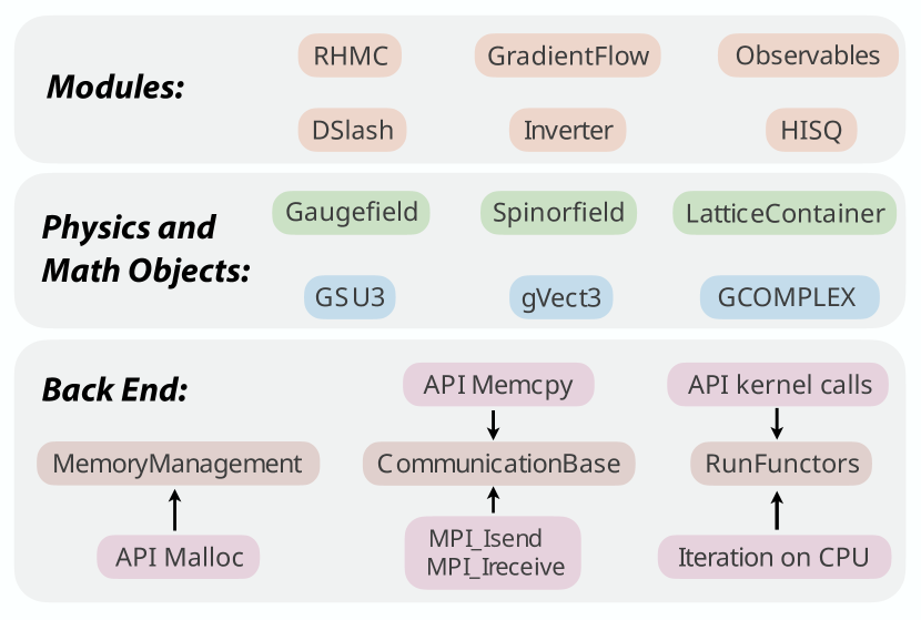
Figure 1: Diagram illustrating the code’s inheritance hierarchy by listing some example classes. Generally speaking, modules inherit from physics and math objects, which in turn inherit from the back end. Image adapted from Ref. [36].

SIMULATeQCD is a multi-GPU, multi-node lattice code written using C++17 and utilizing the Object Oriented Paradigm (OOP) and modern C++ features. In the following we discuss key ideas guiding the code’s design and mention some of the tools already available for lattice calculations. In order to adequately address the challenges highlighted in Section 1, we have worked to develop code that

1. is high-performing;

2. works efficiently on multiple GPUs and nodes;

3. is flexible to changing architecture and hardware; and

4. is easy to use for lattice practitioners with intermediate C++ knowledge.

Besides support for multi-GPU via various APIs, the major difference between SIMULATeQCD and its predecessors lies in the clear distinction between organizational levels of the code, where much of the technical details are hidden from the highest level. This allows physicists without advanced C++ or hardware knowledge to write highly efficient code without having to understand low-level subtleties.

At the highest organizational level are the modules, described in Section 3. Here, we strive to write code that closely and obviously mimics mathematical formulas or short descriptive English sentences. The modules utilize general physics and mathematics classes, which sit at an intermediate level. In turn, these classes inherit from classes of the back end, which is the lowest organizational level. An overview of our code’s inheritance scheme is depicted in Fig. 1.

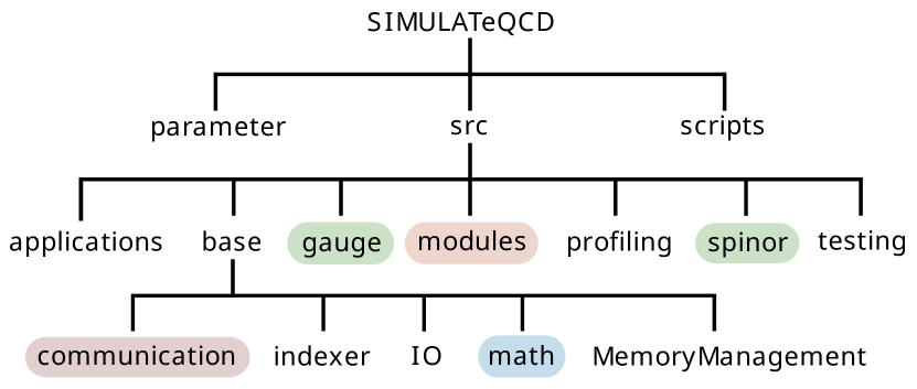
Figure 2: Folder layout of SIMULATeQCD.

The folder structure of SIMULATeQCD is given in Fig. 2. The root directory features the parameter folder, which contains example files that can be used as input for executables. We discuss these files in Section 4.7. The scripts folder contains Bash and Python scripts that assist in using the code, such as scripts that run tests or estimate the memory usage. Finally the src folder contains the main source code, which is further partitioned as follows:

• applications: Ready-to-use applications for generating configurations and carrying out measurements, see Section 2.1.

• base: Low-level code implementation, which is discussed in detail in Section 4.

• gauge: Implementation of objects, described in Section 4.

• modules: Modules that are built up from math and physics objects, such as the classes for carrying out updates. These are described in Section 3.

• profiling: Ready-to-use applications to profile and check the performance of SIMULATeQCD, see
  Section 2.2.

• spinor: Implementation of objects, described in Section 4.

• testing: Ready-to-use applications for testing the code, see Section 2.2.

2.1 Applications

Due to its design strategy, SIMULATeQCD makes it easy for developers to create new multi-GPU applications out of already existing modules. However, many well-tested applications for LQCD calculations already exist. These applications can serve as a starting point for new code, and they have already been used extensively for production in various physics projects. Our applications include, but are not limited to, the following:

• RHMC: Generate 2+1 flavor HISQ gauge configurations using a rational hybrid Monte Carlo algorithm. Utilized in Refs. [37, 17, 16, 14, 15] for $\mu_{B}=0$ and Refs. [38, 39] for pure imaginary $\mu_{B}$. $N_{f}=3$ degenerate quarks at $\mu_{B}=0$ were generated for Ref. [40]. For details see Section 3.1.

• GenerateQuenched: Generate pure gauge configurations with the Wilson gauge action by applying heat bath and over-relaxation updates. Utilized in Refs. [41, 42, 43]. For details see Section 3.1.

• gradientFlow: Integrate the gradient flow equation using the Wilson or Zeuthen action with fixed or adaptive step sizes and measure various gauge constructs at each step. Utilized in Refs. [41, 42, 44, 43, 45].

• gaugeFixing: Fix the gauge of a configuration to the Coulomb or Landau gauge. Can optionally measure various gauge constructs at the end. Utilized in Refs. [46, 47, 48].

• wilsonLinesCorrelator: Measure the trace of the product of two Wilson lines going in opposite time directions separated by a distance $r$. Utilized in Refs. [47, 48].

• sublatticeUpdates: Measure the color-electric correlators and energy-momentum-tensor correlators using multilevel algorithm.

2.2 Testing and profiling

SIMULATeQCD is constantly being expanded and improved by multiple physicists working in multiple places of the code, and it is of utmost importance that physics results and performance remain stable under these changes. To help check and protect against bugs, we have a large suite of tests as well as some profilers. We only allow code to be merged into the main branch when it is confirmed that all executables compile and all tests pass. Changes to lower level code are asked to further demonstrate no significant loss of performance, for which we use the profilers. When a new feature is implemented, we require the implementer to set up a testing script. Testing strategies vary depending on the feature, but they include comparisons to old code; comparisons to analytic results; performing a calculation in another, independent way; and link-by-link checks against trusted configurations.

3 Physics modules

A typical lattice calculation is divided into two main parts: First gauge configurations are generated, then physical observables are measured on the configurations. Many observables are extracted from correlation functions. Sometimes the observables are extremely noisy, and hence it is necessary to employ various noise-reduction techniques. SIMULATeQCD has modules to accomplish all of these tasks, which we discuss in the present section.

3.1 Configuration generation

Gauge configurations are generated via Markov Chain Monte Carlo using Metropolis-type algorithms [49]. To generate the required random numbers we use a hybrid Tausworthe [50, 51].

Currently, SIMULATeQCD can generate pure SU(3) configurations and HISQ configurations with $N_{f}=N_{l}+N_{s}$ for $N_{l}$ light and $N_{s}$ strange dynamical quarks. Non-integer numbers of flavors are supported as well. To enable simulations of four or more degenerate flavors, the fermion determinant was split up into $N_{\rm pf}$ pseudofermion fields, since the rational approximation requires $N_{i}<4$.

$$\prod^{N_{\rm pf}}_{i=1}\left(\frac{\det(\not{D}_{l,i}+m_{l})}{\det(\not{D}_{s,i}+m_{s})}\right)^{\frac{N_{l}}{4N_{\rm pf}}}\prod^{N_{\rm pf}}_{j=1}\left(\det(\not{D}_{s,j}+m_{s})\right)^{\frac{N_{l}+N_{s}}{4N_{\rm pf}}}$$ (1)

Note that $N_{l}$ and $N_{s}$ are input parameters of the rational approximation, while only $N_{\rm pf}$ is an input parameter of SIMULATeQCD. An extension of the code to support different numbers of pseudofermions in the light and strange mass would be straightforward to implement. By default, simulations run with $N_{\rm pf}=1$. Also by default, dynamical quark configurations are generated at $\mu_{B}=0$, but it is also possible to simulate at pure imaginary $\mu_{B}$ [52].

For pure SU(3) we have implemented the standard Wilson gauge action [53], with efficient sampling through heat bath (HB) [54, 55, 56] and over-relaxation (OR) [57, 58] updates. For dynamical fermions, we use the HISQ action [59] and generate configurations using a Rational Hybrid Monte Carlo (RHMC) algorithm [60, 61].

To carry out matrix inversions we use a conjugate gradient algorithm, for which multiple right-hand sides [62] (MRHS), multiple shifts [63], and mixed precision implementations are available to improve performance. The RHMC uses a three-scale integrator [64], which naturally profits from the Hasenbusch trick [65]. By default, the integration uses a leapfrog, but an Omelyan ($2{}^{\rm nd}$ order minimal norm) integrator for the largest scale is also available [66].

HISQ fermions utilize two levels of smearing [67]. The first-level link treatment is

$$c_{1} =1/8$$ (2)

$$c_{3} =1/16$$

$$c_{5} =1/64$$

$$c_{7} =1/384,$$

where $c_{1}$ is the coefficient for the 1-link, and $c_{3}$, $c_{5}$, and $c_{7}$ are for the 3-link staple, 5-link staple, and 7-link staples, respectively. The first-level smeared link is then projected back to U$(3)$ before the application of the second-level smearing. The second level uses

$$c_{1} =1$$ (3)

$$c_{3} =1/16$$

$$c_{5} =1/64$$

$$c_{7} =1/384$$

$$c_{\text{Lepage}} =-1/8$$

$$c_{\text{Naik}} =-1/24+\epsilon/8,$$

where $c_{\text{Naik}}$ and $c_{\text{Lepage}}$ are the coefficients for the Naik and Lepage terms [68]. This is the same link treatment used by the MILC collaboration [69]. We use the HISQ/tree action, which is a tree-level improved Lüscher-Weisz action in the gauge sector [70]. The relative weights of the plaquette and rectangle terms are

$$c_{\text{plaq}} =5/3,$$ (4)

$$c_{\text{rect}} =-1/12.$$

The value of the parameter in the force cut-off that we use in the force filter is $\delta=10^{-5}$ [69]. This value may need to be tuned when one wants to perform QCD thermodynamics calculations very close to the chiral limit.

3.2 Measurement of observables

Implementations for physical observables consisting of gauge constructs include: the Polyakov loop, Polyakov loop correlators in the singlet, average, and octet channels, the chiral condensate, the topological charge, topological charge density, its correlator, and the Weinberg operator

calculated from the field strength tensor and $\order{a^{2}}$- and $\order{a^{4}}$-improved field strength tensor [71], the plaquette, the clover, the color-electric and color-magnetic correlator, and energy-momentum tensor correlators.

There is a method that measures the chiral condensate for a small number of random vectors. This method is used to report in situ measurements of the chiral condensate while the RHMC is running. Hadronic correlation functions along any direction are implemented using HISQ fermions (point sources) to compute, for example, (screening) masses of mesons in various channels. We also support measurement of Taylor coefficients for the expansion of $\log\mathcal{Z}_{\rm QCD}$ in $\mu_{B}/T$.

Some observables, such as certain Polyakov loop correlators, must be measured in special gauges. To this end, Coulomb and Landau gauge fixing are implemented via over-relaxation [72] updating, with over-relaxation parameter $\omega=1.3$.

3.3 Noise reduction

For applications where one needs to attenuate short-distance gauge fluctuations, we have implemented the gradient flow [73] with Wilson and Symanzik-improved actions [74] (Zeuthen flow). The numerical integration is carried out using a third-order Runge-Kutta method for Lie groups [75, 76] with fixed or adaptive step sizes. The blocking method [44] can be a good supplement to the gradient flow method to substantially improve the signal-to-noise ratio of bosonic correlators or other correlators with disconnected contributions. It is implemented by breaking two planes at different time slices into bins and computing bin-bin correlators.

We have also implemented hypercubic blocking (HYP) smearing [77], which uses hypercubic fat links to minimize the largest fluctuations of the plaquette by maximizing the smallest plaquettes.

The multi-level algorithm [78, 79] is implemented by incorporating sublattice updates and observable calculation. The lattice in the temporal direction is divided uniformly into sublattices. Within each sublattice, HB and OR updates are performed in parallel several times followed by a measuring of the observable. At the moment the Polyakov loop, color-electric correlators, and energy-momentum tensor correlators can be measured using this algorithm.

3.4 General calculation of all-to-all correlators

One of the most common types of observable needed to calculate in lattice computations is the correlator. Generically a correlator is an operator

$$\text{correlator}=\expectationvalue{f(A,B;r)}\Big{|}_{D},$$ (5)

where $A$ and $B$ are some operators evaluated at space-time positions $x$ and $y$ belonging to the domain $D$, $r=|x-y|$, and $f$ is an arbitrary function of $A$ and $B$. In order to calculate this quantity, one has to find all possible pairs of sites at a given $r$; hence we have implemented a general framework.

The class handles these general calculations. The fundamental method is the method

$$\texttt{correlateAt<f>("domain",A,B)}.$$ (6)

This correlates arrays and of arbitrary type according to the correlator archetype . The site pairing scheme is controlled by . This returns an array of $\expectationvalue{f(A,B)}$ indexed by $r^{2}$. At the moment, this framework is only available for single GPU use.

4 Low-level implementation

The back end of SIMULATeQCD operates close to the hardware level to achieve high performance, for example through dedicated classes for memory management and communication between host and devices, as lattice applications are usually bound by bandwidth. The four-dimensional lattice also needs to be translated to one-dimensional memory, which is handled by an indexing class. Furthermore, there is a class that maps sets of lattice sites to GPU threads, such that operations on multiple sites are run in parallel. The big advantage of this class is that the operations on each site can be written as high-level functors that do not require any knowledge about the specifics of GPU programming. The back end of the code is finally completed with classes that manage file input/output and logging.

4.1 Allocating and deallocating memory

The memory demands for lattice calculations can increase with increasing lattice size in a nontrivial way, depending on the algorithm being used. Thus, for complex applications it can be difficult to keep track of all dynamically allocated memory on both host and device, especially since GPU memory allocation and deallocation has to be handled via the appropriate API, depending on the hardware. Additionally, to avoid memory leaks, memory should be automatically deallocated when appropriate. Finally, memory (de)allocation can take a non-negligible amount of time, so one can gain a performance boost by allowing large chunks of memory to be shared.

To address these issues, we developed the centralized class, which manages and knows about all instances of dynamically allocated memory. This is accomplished through the member class, which can hold the raw pointer to dynamically allocated memory along with API-independent wrappers for memory allocation and deallocation. objects are pointed to by our custom smart pointer, the . A is labelled by a SmartName, a descriptive string chosen by the user that by default prevents that two pointers point to the same memory. However, the memory can be shared by choosing a SmartName beginning with the string SHARED. Each object also informs the when it is created and destroyed.

The is never explicitly instantiated, as all necessary methods are static. This includes those needed to create new dynamic memory, destroy it, and report to the user which dynamic memory exists, along with its size and SmartName.

4.2 Communication

To work with multiple devices, SIMULATeQCD splits a lattice into multiple sublattices, with partitioning possible along any space-time direction. Each sublattice is given to a single GPU, and we call this sublattice the bulk. In addition, the GPU holds a copy of the outermost borders of neighboring sublattices, which we call the halo. This halo is necessary because many measurement and update processes are stencil operations, which means that a calculation performed at some site may need information from a neighboring sublattice. Every so often, information from all sublattices must be injected into their neighbors’ halos. A schematic drawing of the exchange of halo information between different GPUs is shown in Fig. 3 (top).

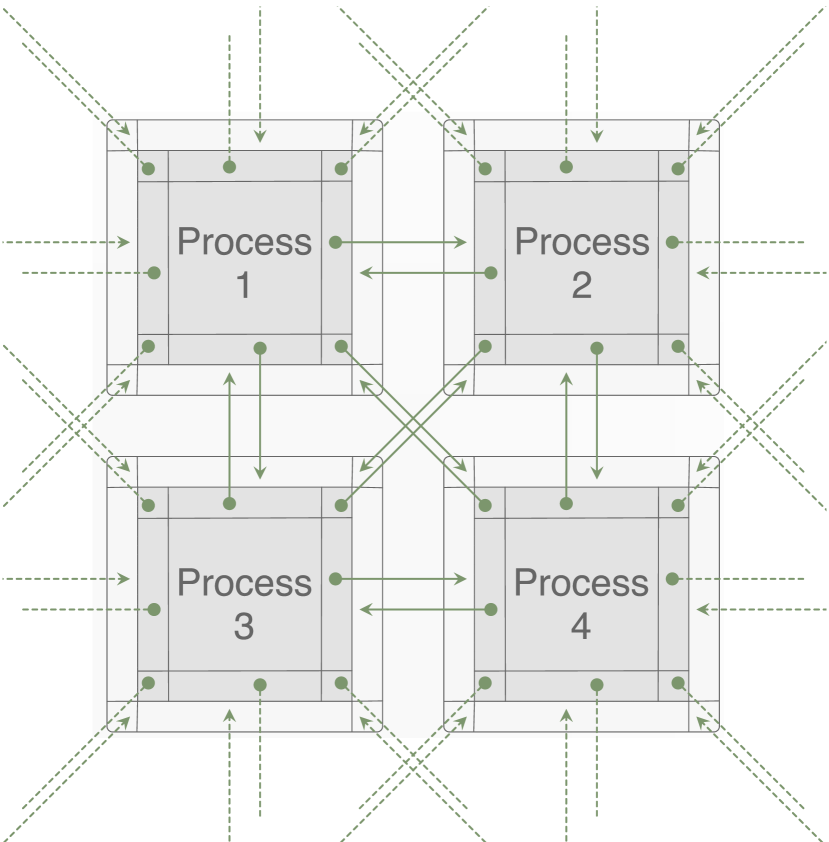
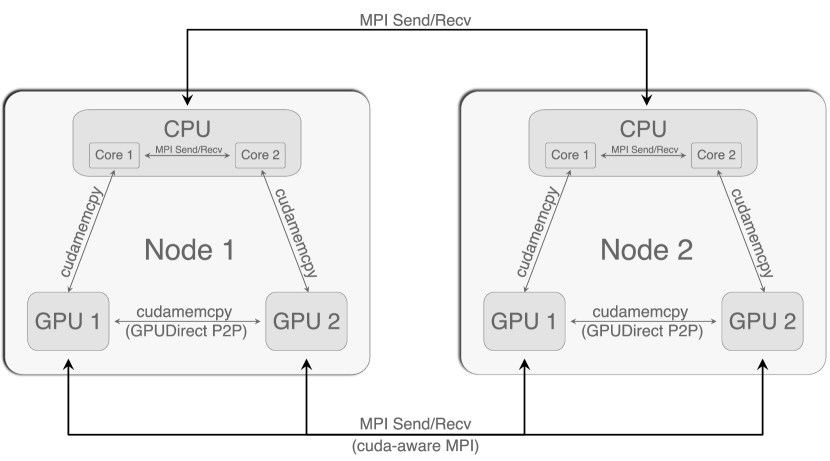
Figure 3: Top: Schematic halo exchange for four processes in two dimensions, each process containing a sublattice. The bulk is indicated by the dark gray squares, and the halo is indicated by light grey squares. Copies of sites located near the borders of the bulk, set off here by solid grey lines, are stored in the halos. Information starts at solid green circles and is injected into the halos following the arrows. Dotted lines indicate injections following periodic boundary conditions. Bottom: Diagram summarizing different possible communication channels for hardware. Images taken from Ref. [1].

Figure 4: Dependence structure of the and on communication classes.

List of Listings 1 An example functor, , utilizing functor syntax. It is templated to allow for arbitrary precision , to run on GPU with , for arbitrary , and to allow the to use arbitrary . This functor takes a object as argument, whose elements are accessed in memory through the , set to point to the accessor in the initializer list. The argument of indicates that this functor will be iterated over objects. We indicate with that we run over both even and odd parity sites. The method multiplies all links starting at , following a path in the specified directions. We compute the real part of the trace with . Due to our functor syntax, all lattice splitting, communication, and distribution to GPU threads is done behind the scenes.

List of Listings 2 Using an iterator to calculate the plaquette with the functor given in Listing 1. We instantiate our object and a , which is needed for the reduction across threads and nodes. Our iterator, will assign each in the bulk of a sublattice to a GPU thread; hence it needs to have $N_{\sigma,\hskip 0.28453pt\text{sub}}^{3}\times N_{\tau,\hskip 0.28453pt\text{sub}}=\texttt{vol4}$ elements. The reduction happens over the global lattice, so in the last time we normalize by $N_{\sigma}^{3}\times N_{\tau}$, three colors, and six plaquettes per site in four dimensions.

List of Listings 3 Sketch of low level functor and iterator implementation. API-dependent constructions are wrapped inside and methods. The user can decide at compile time whether to use the CUDA or HIP API, which is implemented here using . These methods are templated to allow memory access to an arbitrary return type using memory accessor . The operation is at this level completely unspecified; it will be defined at a higher level through a functor, for example the plaquette functor shown in Listing 1. The types and respectively translate from GPU thread index to input memory index and from input to output memory index. The object in is set to to allow use with arbitrary indexing object, for example the and objects defined in Section 4.3.

List of Listings 4 An excerpt from the implementation showing the specialization of to add two “Class” objects.

Communication between multiple CPUs and multiple nodes is handled with MPI, which also allows for communication between multiple GPUs. We use MPI two-sided communication. For NVIDIA hardware, we handle communication between GPUs on the same node using CUDA GPUDirect P2P. CUDA-aware MPI is used for internode communication. We boost performance by allowing the code to carry out certain computations while communicating, such as copying halo buffers into the bulk, whenever possible. An example of different communication channels for two nodes is given in Fig. 3 (bottom).

Wrappers for methods used in these various communication libraries are collected in the class. The will also detect whether CUDA-aware MPI or GPUDirect P2P is available, and if it is, use it (or both) automatically since these channels have less communication overhead than standard MPI.

Halo communication proceeds by first copying halo information contiguously into a buffer. This requires translating from the sublattice’s indexing scheme to the buffer’s indexing scheme. The class provides offsets for different halo segments (stripe halo, corner halo, etc). These offsets and the buffer base pointer are used to place the halo data at the correct position in the buffer. An example for the corner halo would be:

$$\text{corner buffer pointer}={}$$ buffer base pointer

$$+\text{corner halo offset}.$$

The class is the lowest level class from which all objects that need to communicate across sublattices, such as the introduced in the next section, inherit. It uses the to allocate memory for the buffer, uses the to translate the local index to the buffer index, copies information into the buffer, and finally uses the to carry out the exchange. This chain of dependencies is illustrated in Fig 4.

4.3 Indexing and fields

LQCD is restricted to a finite region of discretized 4-$d$ space-time with spatial extensions $N_{\sigma}$ and temporal extension $N_{\tau}$, such that the total number of sites is $N_{\sigma}^{3}\times N_{\tau}$. Sites are separated by the lattice spacing $a$. These quantities are related to the physical volume by $V=(aN_{\tau})^{3}$ and temperature by $T=1/aN_{\tau}$. Each site has coordinates $(x,y,z,t)\in\mathbb{Z}^{4}$ with $x,y,z\in\{0,...,N_{\sigma}-1\}$ and $t\in\{0,...,N_{\tau}-1\}$, and each direction is represented by $\mu\in\{0,1,2,3\}$. The gluon fields $U_{\mu}(x)\in\operatorname{SU}(3)$ are the links, and staggered fermion (spinor) field objects $\chi^{c}(x)\in\mathbb{C}^{3}$ [3], where $c\in\{{0,1,2}\}$, rest on the sites. Links are implemented straightforwardly as $3\times 3$ complex matrices and the spinor fields as complex 3-vectors. These fundamental variables are stored in and objects, which contain arrays of links and spinors, respectively. objects have periodic boundary conditions (BCs) while objects have periodic spatial BCs and an anti-periodic time BC.

Our site indexing is done in lexicographic order, but for many purposes, it is convenient to characterize sites with an even/odd parity.

For applications where this is the case, it is more efficient to organize sites in memory such that all even sites are in the first half of the memory and all odd sites are in the second half. Therefore we convert the 4-$d$ coordinate of a site to the 1-$d$ memory index as

$$\text{index}= ~{}\frac{1}{2}\left(x+yN_{\sigma}+zN_{\sigma}^{2}+tN_{\sigma}^{3}\right)$$ (7)

$$+\frac{1}{2}N_{\sigma}^{3}N_{\tau}\left(x+y+z+t\right)\bmod 2.$$

Building up from this, links are indexed by

$$\text{index}= ~{}\frac{1}{2}\left(x+yN_{\sigma}+zN_{\sigma}^{2}+tN_{\sigma}^{3}\right)$$ (8)

$$+\frac{1}{2}N_{\sigma}^{3}N_{\tau}\left(x+y+z+t\right)\bmod 2+\mu N_{\sigma}^{3}N_{\tau}.$$

When using multiple GPUs, similar formulae hold for the sublattices, except that the extensions are replaced by $N_{\sigma}\to N_{\sigma,\hskip 0.28453pt\text{sub}}$ and $N_{\tau}\to N_{\tau,\hskip 0.28453pt\text{sub}}$. Hence we distinguish between the local index and global index. Moreover, as explained in the previous section and as depicted in Fig. 3, information about neighboring fields is stored in a halo surrounding the bulk. Therefore besides bulk indexing, each sub-lattice has so-called “full” indices that include the halos. This scheme is computed by

$$\text{index}_{\texttt{\hskip 0.28453ptFull}}= ~{}\frac{1}{2}\left(x+yN_{x}+zN_{x}N_{y}+tN_{x}N_{y}N_{z}\right)$$ (9)

$$+\frac{1}{2}N_{x}N_{y}N_{z}N_{t}\left(x+y+z+t\right)\bmod 2,$$

while the links are indexed by

$$\text{index}_{\texttt{\hskip 0.28453ptFull}}= ~{}\frac{1}{2}\left(x+yN_{x}+zN_{x}N_{y}+tN_{x}N_{y}N_{z}\right)$$ (10)

$$+\frac{1}{2}N_{x}N_{y}N_{z}N_{t}(x+y+z+t)\bmod 2$$

$$+\mu N_{x}N_{y}N_{z}N_{t},$$

with

$$N_{i}= ~{}N_{\sigma}+H_{i},\qquad i\in x,y,z,$$

$$N_{t}= ~{}N_{\tau}+H_{t},$$

where $H_{i}$, $H_{t}$ are the halo depths in different directions.

In order to abstract these difficulties away from the user, we have implemented objects. A object holds all information about a site, including its coordinates and index in the local, global, and full context. All methods for calculating indices, coordinates, and movement along the lattice are contained in the class. The user can easily control odd/even indexing by passing a template parameter, which can be set to , , or . Similarly, the class holds all information about link indexing.

4.4 Functor syntax

Much of the effort in this code goes into abstracting away highly complex parallelization, which depends on the API, whether GPUs or CPUs are used, the number of processes, the node layout being used, and so on. In order to accomplish this for the general case, we have implemented a system where one can iterate an arbitrary operation that depends on arbitrary arguments over an arbitrary set of coordinates.

One common task in lattice calculations is to perform the same calculation on each lattice site, which involves link variables at or close to that site, for example, computing the plaquette,

$$U^{\square}_{\mu\nu}(x)=U_{\mu}(x)U_{\nu}(x+a\hat{\mu})U^{\dagger}_{\mu}(x+a\hat{\nu})U^{\dagger}_{\nu}(x).$$ (11)

An example kernel computing the plaquette is shown in 1. The code for the kernel is wrapped in a functor, i.e. a with its overloaded, which in this case takes a object as argument. The functor is passed to a function which we call an iterator. This function iterates over all required lattice sites and calls the functor on each one, thereby distributing the calls on the available computing resources. An example usage of this is given in Listing 2, where the iterator is called using the functor as a template parameter. By using functors as template parameters for iterators, we can conveniently iterate arbitrary calculations over sites, without the need to write specialized code each time.

Iterators like , which calls the

’s at bulk sites, inherit from the

class, which contains the lowest-level methods that iterate functors over the desired target set. In Listing 3 we provide sketches of the most salient methods in the class, namely , which applies a functor to a or object, and , which carries out using CUDA or HIP.

If we are not using GPUs and just evaluate the computation kernel on multiple CPUs, then the iterator method iterates sequentially over the sites/links of a sublattice using -loops, with one sublattice per CPU core in parallel. But if we use GPUs, then there are no -loops. Instead, the computation of each iteration of these nested -loops will also be parallelized on threads of the GPUs. For example with the plaquette computation,

$${\rm number\ of\ GPU\ threads}=\frac{N_{\sigma}^{3}\times N_{\tau}}{{\rm number\ of\ GPUs}}$$ (12)

are spawned, where each thread is doing the work corresponding to a certain site.

As mentioned in Section 4.3, we index sites and links through and objects, respectively; hence one usually passes either a or object to the functor. The class also contains several methods that tell the iterator how to translate from these objects to GPU thread indices.

4.5 Expression templates

To facilitate an efficient but intuitive composition of math expressions involving basic physics objects such as spinorfields and gaugefields, we implement general math operations such as additions, subtractions, multiplications and divisions via expression templates [80].

We define a set of functions such as and that, instead of performing the corresponding math operation, return a functor that holds the information to carry out the desired calculation. The execution of this calculation is triggered by the copy assignment operator (=) of the basic physics object, which passes the functor to an method.

Using the “Substitution failure is not an error” (SFINAE) principle, we specialize the struct for different type combinations such as “Class + Class” and “Class + scalar”. In this context, “Class” means an object that has a -method and operator() defined. This object could be a , a or another . Nesting of expressions such as $a\cdot b+c\cdot d$, where $a,b,c,d$ are physics objects, and combinations of operators and scalars such as $(a\cdot b)\cdot 2.0$ are also implemented. This highly templated, low-level code allows users to write high-level physics code involving s, s, etc. that closely resembles familiar mathematical equations while also avoiding superfluous evaluations of temporary expressions.

Listing 4 shows an excerpt of the implementation detailing the specialization of additions of two class objects.

4.6 Instantiation macros

In order to make our code as flexible as possible and to reduce code repetition, we make extensive use of C++ templates. At the same time, we would like to put kernel implementations into cpp files in order to reduce build times. This often requires explicitly instantiating all possible template parameter combinations, which is repetitive, messy, and tedious.

In order to help streamline this process we make use of explicit instantiation macros, which help automate the instantiation of the most commonly used template parameters. For example, one can instantiate a generic class for all possible precisions (P), halo depths (H), and gauge field compression template parameters (C) by using .

4.7 Parameter handling and IO

Parameter files hold input parameters such as quark masses and couplings, as well as information like the lattice dimension, random number seed, etc. These are implemented through our class . More specialized parameter classes, for example the parameter class for the RHMC, inherit from this. Default parameter files are in the parameter folder mentioned in Section 2, but one can also pass a custom parameter file as argument to any executable.

Another challenge facing large-scale LQCD projects is finding the storage space for petabytes of configurations. Furthermore, configurations are highly flexible to many kinds of measurements, so it is conducive for open science to store these configurations in a standardized, accessible way, find long-term storage elements on which to place them, and to responsibly collect and curate metadata to help lattice practitioners find these configurations, for example through a search tool. In this context, it is nowadays stressed that scientific data should be FAIR [81].

The most well equipped scheme to effectively carry out such a task in LQCD is the International Lattice Data Grid (ILDG) [82], which provides a common format and metadata scheme in order to facilitate configuration sharing among lattice groups, and which is now being resuscitated [83]. ILDG configuration binaries must be written out in LIME format [84] and packaged together with a corresponding XML metadata file that validates against the QCDml [85] schema. To this end we allow that our configurations comply with the format of the ILDG, written out as LIME files. To assist with forming a QCDml file, one can pass optional ILDG-compliant parameters to the class that are printed to the standard output. These metadata can then be captured by custom scripts.

In addition to ILDG format, SIMULATeQCD also has support for MILC [86], NERSC, and openQCD [87] configuration formats, three other commonly used formats in the lattice community.

Figure 5: Performance of the HISQ Dirac operator with varying number of RHS vectors on a single JUWELS Booster node.

Figure 6: Scaling of HISQ Dirac operator with a single RHS on Perlmutter. Top: Strong scaling for a $96^{4}$ lattice. Bottom: Weak scaling for a $32^{4}$ local lattice.

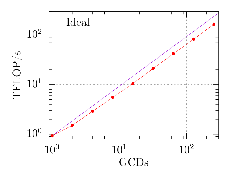
Figure 7: Scaling of HISQ Dirac operator with single RHS on Frontier. Top: Strong scaling for a $96^{4}$ lattice. Bottom: Weak scaling for a $32^{4}$ local lattice.

5 Performance

In order to save memory without losing too much precision, especially in performance-critical situations, we use link compression. For instance our HISQ smearing implementation needs several temporary objects, and for the Naik term it is not necessary to represent a link with 18 reals. Uncompressed gauge fields can be reconstructed for example through unitarization.

When generating HISQ configurations for typical parameters, about 60% of our RHMC run time is spent inverting the Dirac matrix via conjugate gradient, and in it, applying the $\not{D}$ operator to a vector is the most performance-critical kernel. Hence this and related kernels are important benchmarks. The kernel’s performance is limited by the available memory bandwidth, but its arithmetic intensity can be increased by applying the gauge field to multiple RHS simultaneously. Furthermore, it benefits from gauge field compression. Only a subset of the link matrix entries are stored in memory, and the missing entries are recomputed from the stored ones based on the symmetries, either $\operatorname{SU}(3)$ or $\operatorname{U}(3)$, of the link matrix.

To improve performance, we overlap certain computations, such as the kernels that prepare halo buffers, with communication.

5.1 Benchmarks on A100 GPUs

The performance of our multi-RHS Dslash implementation for varying number of RHS and GPUs is given in Fig. 5. It was performed on Juwels Booster, where each node is configured with 4 NVIDIA A100 GPUs. We see performance improvements from Gaugefield re-use with increasing number of RHS up to about 8 RHS, regardless of the number of GPUs. The scaling on a single node is close to ideal and we achieve a maximum of about 11.4 TFLOP/s on a full node while using 8 RHS.

Profiling the Dslash kernel using NVIDIA’s Nsight compute software reveals that we achieve a memory throughput of up to 1.36 TB/s on a single A100 GPU, thus coming very close to the cards peak memory bandwidth of about 1.55 TB/s.

In Fig. 6 we show strong- and weak-scaling benchmarks of our HISQ DSlash on Perlmutter, which, like Juwels Booster, has 4 NVIDIA A100 GPUs per node. Nodes are interconnected via HPE Slingshot 11 fabric and have 4 NICs providing 25GB/s bandwidth each. We find good weak scaling on this system up to 256 GPUs. A slight decrease in speedup can be seen as soon as node-to-node communication starts. Strong scaling benchmarks with a $96^{4}$ global lattice size start deviating from ideal scaling earlier. As the local lattice sizes and thus the compute workloads of the individual GPUs keep getting smaller, hiding the HISQ DSlash’s communication becomes increasingly difficult.

5.2 Preliminary Benchmarks on MI250X GPUs

In Fig. 7 we show HISQ DSlash benchmarks on Frontier. This system is configured with 4 AMD MI250X per node. Each MI250X is comprised of 2 Graphic Compute Dies (GCDs); i.e. there are 8 GCDs per node. GCDs inside an MI250X are connected via Infinity Fabric with 200GB/s bi-directional bandwidth, and the 4 MI250X cards on a node are connected via Infinity Fabric with bi-directional bandwidths between 50-100GB/s depending on their arrangement. Nodes are connected via four HPE Slingshot NICs each providing 25GB/s of bandwidth. The weak scaling benchmark with a $32^{4}$ local lattice volume shows close to ideal scaling all the way up to 256 GCDs. Going from 8 GCDs to 16 GCDs shows no significant drop in speedup although node-to-node communications kick in. The strong scaling benchmark scales well up until 16 GCDs. After that point, communication can no longer be hidden effectively and the speedup decreases. First tests on LUMI-G produced comparable single GCD performance as that in Frontier. We note that the single GPU performance achieved on MI250X is currently lagging behind what we would expect given the cards specifications. A single GCD has a memory bandwidth similar to that of a single A100 GPU, and we would therefore expect to see performance differences between both to be smaller. As more machines equipped with MI250X cards transition from early access into production mode and as profiling tools for AMD hardware mature, we are investigating what is causing this decreased performance and continue to optimize our code for this new hardware.

no. of RHS	4 GPUs	3 GPUs	2 GPUs	1 GPU
1	4.73079	3.64066	2.43864	1.27963
2	7.66433	5.93165	3.95775	2.10292
3	9.3739	7.30559	4.89197	2.66587
4	10.5115	8.20125	5.54996	3.06388
5	11.0659	8.64023	5.87168	3.27174
6	11.317	8.82256	6.06521	3.3924
7	11.0128	8.6586	5.98085	3.37701
8	11.4201	9.00431	6.27061	3.57343
9	10.7651	8.54542	5.94003	3.36035
10	11.1947	8.86835	6.18	3.51152

Table 1: Data for Figure 5, showing the performance of the HISQ Dirac operator on a JUWELS Booster node for different numbers of right hand side vectors (RHS).

strong scaling		weak scaling
GPUs	TFLOP/s	GPUs	TFLOP/s
1	-	1	1.35746
4	5.06892	4	4.53759
8	8.58352	8	6.85441
16	12.5533	16	9.87794
32	19.5635	32	17.9565
64	35.0211	64	33.0596
128	47.6174	128	63.4786
256	96.4686	256	120.445

Table 2: Data for Figure  6, showing the strong and weak scaling of the HISQ Dirac operator on Perlmutter with a $96^{4}$ global lattice and $32^{4}$ local lattice, respectively.

strong scaling		weak scaling
GCDs	TFLOP/s	GCDs	TFLOP/s
1	-	1	0.92974
2	1.63049	2	1.51439
4	3.00675	4	2.89454
8	4.69513	8	5.57654
16	9.17246	16	10.5269
32	12.6743	32	21.2049
64	21.8216	64	42.1544
128	35.3419	128	82.5013
256	40.6282	256	165.718

Table 3: Data for Figure  7, showing the strong and week scaling of the HISQ Dirac operator on Frontier with a $96^{4}$ global lattice and $32^{4}$ local lattice, respectively.

6 Outlook

We presented SIMULATeQCD, a multi-GPU, multi-node lattice code that allows simulation of dynamical fermions using the HISQ action and works for both NVIDIA and AMD back ends. We chose the HISQ action since it is widely used for state-of-the-art, high-statistics QCD studies. In writing SIMULATeQCD, we sought to write clean code that is highly modularized, so that anyone with modest knowledge of C++ can get started writing production code right away. We believe this is an important and sometimes overlooked characteristic of code in a lattice context, where personnel and hardware are constantly changing. At the same time, we did our best to ensure good performance by writing code close to the hardware that is both mindful of and flexible to the computing system. We leveraged functor syntax to balance both of these needs. SIMULATeQCD has many production-ready applications, which are listed in Section 2.1. We gave some details on the implementation of our physics modules in Section 3 for easy and transparent reference in the future.

What exists in SIMULATeQCD presently mostly includes code that has been relevant to HotQCD projects. One of the most important characteristics of SIMULATeQCD is that it is relatively straightforward to implement new algorithms; hence wherever there is desire and manpower, our code can be extended to suit the needs of a new project in an uncomplicated, undemanding way. One of the obvious avenues of extension for SIMULATeQCD on the physics side includes implementation of other 4-$d$ actions, such as the Wilson action for fermions. While the code already works for $N_{f}=2+1$ and degenerate $N_{f}$ systems, some work is still needed to include a dynamical charm quark. A relatively new feature allows measurement of Taylor coefficients of the pressure, however this still needs deflation to be suitable for efficient use with lighter quarks. Finally, the code is already relatively integrated with ILDG, and this should ideally be continued in parallel with the ILDG revival.

Turning to low-level implementation, machines such as Aurora will utilize Intel GPUs, so it will be valuable to introduce also a Sycl back end. Along this vein, while most modules require a GPU back end, everything can also be compiled and run on CPUs only by adding a few macros, which so far has been done for a few selected modules.

CRediT authorship contribution statement

Lukas Mazur: Conceptualization, Methodology,
Project administration, Software, Validation. Writing – Review & Editing. Dennis Bollweg: Software, Validation. Writing – Review & Editing. David A. Clarke: Software, Validation. Writing – Original Draft, Review & Editing. Luis Altenkort: Software, Validation. Writing – Review & Editing. Olaf Kaczmarek: Conceptualization, Supervision, Project administration, Funding acquisition. Rasmus Larsen: Software. Hai-Tao Shu: Software. Jishnu Goswami: Software. Philipp Scior: Software, Validation. Hauke Sandmeyer: Conceptualization, Software. Marius Neumann: Software. Henrik Dick: Software. Sajid Ali: Software. Jangho Kim: Software. Christian Schmidt: Software, Supervision, Funding acquisition. Peter Petreczky: Writing – Review & Editing. Swagato Mukherjee: Supervision,
Funding acquisition.

References

- [1] L. Mazur, Topological Aspects in Lattice QCD, Ph.D. thesis, Bielefeld U. (2021). doi:10.4119/unibi/2956493.
- [2] SIMULATeQCD public code repository, https://github.com/LatticeQCD/SIMULATeQCD. doi:10.5281/zenodo.7994983.
- [3] J. B. Kogut, L. Susskind, Hamiltonian Formulation of Wilson’s Lattice Gauge Theories, Phys. Rev. D 11 (1975) 395–408. doi:10.1103/PhysRevD.11.395.
- [4] A. S. Kronfeld, Lattice Gauge Theory with Staggered Fermions: How, Where, and Why (Not), PoS LATTICE2007 (2007) 016. arXiv:0711.0699, doi:10.22323/1.042.0016.
- [5] C. Bernard, M. Golterman, Y. Shamir, Effective field theories for QCD with rooted staggered fermions, Phys. Rev. D 77 (2008) 074505. arXiv:0712.2560, doi:10.1103/PhysRevD.77.074505.
-
[6]
K. Orginos,
Innovations
in lattice QCD algorithms, J. Phys.: Conf. Ser. 46 (2006) 132–141.
doi:10.1088/1742-6596/46/1/018.
URL https://iopscience.iop.org/article/10.1088/1742-6596/46/1/018 - [7] E. Follana et al. [HPQCD, UKQCD collaboration], Highly improved staggered quarks on the lattice, with applications to charm physics, Phys. Rev. D 75 (2007) 054502. arXiv:hep-lat/0610092, doi:10.1103/PhysRevD.75.054502.
- [8] A. Bazavov, et al., The chiral and deconfinement aspects of the QCD transition, Phys. Rev. D 85 (2012) 054503. arXiv:1111.1710, doi:10.1103/PhysRevD.85.054503.
- [9] H.-T. Ding, F. Karsch, S. Mukherjee, Thermodynamics of strong-interaction matter from Lattice QCD, Int. J. Mod. Phys. E 24 (10) (2015) 1530007. arXiv:1504.05274, doi:10.1142/S0218301315300076.
- [10] C. Schmidt, S. Sharma, The phase structure of QCD, J. Phys. G 44 (10) (2017) 104002. arXiv:1701.04707, doi:10.1088/1361-6471/aa824a.
- [11] J. N. Guenther, Overview of the QCD phase diagram: Recent progress from the lattice, Eur. Phys. J. A 57 (4) (2021) 136. arXiv:2010.15503, doi:10.1140/epja/s10050-021-00354-6.
- [12] A. Bazavov, et al., Chiral crossover in QCD at zero and non-zero chemical potentials, Phys. Lett. B 795 (2019) 15–21. arXiv:1812.08235, doi:10.1016/j.physletb.2019.05.013.
- [13] A. Bazavov, et al., Equation of state in ( 2+1 )-flavor QCD, Phys. Rev. D 90 (2014) 094503. arXiv:1407.6387, doi:10.1103/PhysRevD.90.094503.
- [14] D. Bollweg, J. Goswami, O. Kaczmarek, F. Karsch, S. Mukherjee, P. Petreczky, C. Schmidt, P. Scior, Taylor expansions and Padé approximants for cumulants of conserved charge fluctuations at nonvanishing chemical potentials, Phys. Rev. D 105 (7) (2022) 074511. arXiv:2202.09184, doi:10.1103/PhysRevD.105.074511.
- [15] D. Bollweg, D. A. Clarke, J. Goswami, O. Kaczmarek, F. Karsch, S. Mukherjee, P. Petreczky, C. Schmidt, S. Sharma, Equation of state and speed of sound of (2+1)-flavor QCD in strangeness-neutral matter at non-vanishing net baryon-number densityarXiv:2212.09043.
- [16] D. Bollweg, J. Goswami, O. Kaczmarek, F. Karsch, S. Mukherjee, P. Petreczky, C. Schmidt, P. Scior, Second order cumulants of conserved charge fluctuations revisited: Vanishing chemical potentials, Phys. Rev. D 104 (7). arXiv:2107.10011, doi:10.1103/PhysRevD.104.074512.
- [17] A. Bazavov, et al., Skewness, kurtosis, and the fifth and sixth order cumulants of net baryon-number distributions from lattice QCD confront high-statistics STAR data, Phys. Rev. D 101 (7) (2020) 074502. arXiv:2001.08530, doi:10.1103/PhysRevD.101.074502.
- [18] A. Bazavov, et al., Skewness and kurtosis of net baryon-number distributions at small values of the baryon chemical potential, Phys. Rev. D 96 (7) (2017) 074510. arXiv:1708.04897, doi:10.1103/PhysRevD.96.074510.
- [19] H. T. Ding, S. Mukherjee, H. Ohno, P. Petreczky, H. P. Schadler, Diagonal and off-diagonal quark number susceptibilities at high temperatures, Phys. Rev. D 92 (7) (2015) 074043. arXiv:1507.06637, doi:10.1103/PhysRevD.92.074043.
- [20] A. Bazavov, H. T. Ding, P. Hegde, F. Karsch, C. Miao, S. Mukherjee, P. Petreczky, C. Schmidt, A. Velytsky, Quark number susceptibilities at high temperatures, Phys. Rev. D 88 (9) (2013) 094021. arXiv:1309.2317, doi:10.1103/PhysRevD.88.094021.
- [21] A. Bazavov, et al., Strangeness at high temperatures: from hadrons to quarks, Phys. Rev. Lett. 111 (2013) 082301. arXiv:1304.7220, doi:10.1103/PhysRevLett.111.082301.
- [22] A. Bazavov, et al., Fluctuations and Correlations of net baryon number, electric charge, and strangeness: A comparison of lattice QCD results with the hadron resonance gas model, Phys. Rev. D 86 (2012) 034509. arXiv:1203.0784, doi:10.1103/PhysRevD.86.034509.
- [23] D. Bala, O. Kaczmarek, R. Larsen, S. Mukherjee, G. Parkar, P. Petreczky, A. Rothkopf, J. H. Weber, Static quark-antiquark interactions at nonzero temperature from lattice QCD, Phys. Rev. D 105 (5) (2022) 054513. arXiv:2110.11659, doi:10.1103/PhysRevD.105.054513.
- [24] B. Chakraborty, C. T. H. Davies, B. Galloway, P. Knecht, J. Koponen, G. C. Donald, R. J. Dowdall, G. P. Lepage, C. McNeile, High-precision quark masses and QCD coupling from lattice QCD, Phys. Rev. D 91 (5) (2015) 054508. arXiv:1408.4169, doi:10.1103/PhysRevD.91.054508.
- [25] A. Bazavov, F. Karsch, Y. Maezawa, S. Mukherjee, P. Petreczky, In-medium modifications of open and hidden strange-charm mesons from spatial correlation functions, Phys. Rev. D 91 (5) (2015) 054503. arXiv:1411.3018, doi:10.1103/PhysRevD.91.054503.
- [26] P. Petreczky, J. H. Weber, Strong coupling constant and heavy quark masses in ( 2+1 )-flavor QCD, Phys. Rev. D 100 (3) (2019) 034519. arXiv:1901.06424, doi:10.1103/PhysRevD.100.034519.
- [27] A. Bazavov, et al., Meson screening masses in (2+1)-flavor QCD, Phys. Rev. D 100 (9) (2019) 094510. arXiv:1908.09552, doi:10.1103/PhysRevD.100.094510.
- [28] P. Petreczky, S. Sharma, J. H. Weber, Bottomonium melting from screening correlators at high temperature, Phys. Rev. D 104 (5) (2021) 054511. arXiv:2107.11368, doi:10.1103/PhysRevD.104.054511.
- [29] A. Bazavov, et al., decay from lattice QCD, Phys. Rev. D 100 (3) (2019) 034501. arXiv:1901.02561, doi:10.1103/PhysRevD.100.034501.
- [30] C. T. H. Davies, et al., Windows on the hadronic vacuum polarisation contribution to the muon anomalous magnetic momentarXiv:2207.04765.
- [31] X. Gao, A. D. Hanlon, S. Mukherjee, P. Petreczky, P. Scior, S. Syritsyn, Y. Zhao, Lattice QCD Determination of the Bjorken-x Dependence of Parton Distribution Functions at Next-to-Next-to-Leading Order, Phys. Rev. Lett. 128 (14) (2022) 142003. arXiv:2112.02208, doi:10.1103/PhysRevLett.128.142003.
- [32] A. Bazavov, N. Brambilla, X. G. Tormo, I, P. Petreczky, J. Soto, A. Vairo, Determination of from the QCD static energy: An update, Phys. Rev. D 90 (7) (2014) 074038, [Erratum: Phys.Rev.D 101, 119902 (2020)]. arXiv:1407.8437, doi:10.1103/PhysRevD.90.074038.
- [33] Y. Maezawa, P. Petreczky, Quark masses and strong coupling constant in 2+1 flavor QCD, Phys. Rev. D 94 (3) (2016) 034507. arXiv:1606.08798, doi:10.1103/PhysRevD.94.034507.
- [34] A. Bazavov, N. Brambilla, X. Garcia i Tormo, P. Petreczky, J. Soto, A. Vairo, J. H. Weber, Determination of the QCD coupling from the static energy and the free energy, Phys. Rev. D 100 (11) (2019) 114511. arXiv:1907.11747, doi:10.1103/PhysRevD.100.114511.
- [35] P. Petreczky, J. H. Weber, Strong coupling constant from moments of quarkonium correlators revisited, Eur. Phys. J. C 82 (1) (2022) 64. arXiv:2012.06193, doi:10.1140/epjc/s10052-022-09998-0.
- [36] D. Bollweg, L. Altenkort, D. A. Clarke, O. Kaczmarek, L. Mazur, C. Schmidt, P. Scior, H.-T. Shu, HotQCD on multi-GPU Systems, PoS LATTICE2021 (2022) 196. arXiv:2111.10354, doi:10.22323/1.396.0196.
- [37] D. A. Clarke, O. Kaczmarek, F. Karsch, A. Lahiri, M. Sarkar, Sensitivity of the Polyakov loop and related observables to chiral symmetry restoration, Phys. Rev. D 103 (1) (2021) L011501. arXiv:2008.11678, doi:10.1103/PhysRevD.103.L011501.
- [38] P. Dimopoulos, L. Dini, F. Di Renzo, J. Goswami, G. Nicotra, C. Schmidt, S. Singh, K. Zambello, F. Ziesché, Contribution to understanding the phase structure of strong interaction matter: Lee-Yang edge singularities from lattice QCD, Phys. Rev. D 105 (3) (2022) 034513. arXiv:2110.15933, doi:10.1103/PhysRevD.105.034513.
- [39] F. Cuteri, J. Goswami, F. Karsch, A. Lahiri, M. Neumann, O. Philipsen, C. Schmidt, A. Sciarra, Toward the chiral phase transition in the Roberge-Weiss plane, Phys. Rev. D 106 (1) (2022) 014510. arXiv:2205.12707, doi:10.1103/PhysRevD.106.014510.
- [40] L. Dini, P. Hegde, F. Karsch, A. Lahiri, C. Schmidt, S. Sharma, Chiral phase transition in three-flavor QCD from lattice QCD, Phys. Rev. D 105 (3) (2022) 034510. arXiv:2111.12599, doi:10.1103/PhysRevD.105.034510.
- [41] L. Altenkort, A. M. Eller, O. Kaczmarek, L. Mazur, G. D. Moore, H.-T. Shu, Heavy quark momentum diffusion from the lattice using gradient flow, Phys. Rev. D 103 (1) (2021) 014511. arXiv:2009.13553, doi:10.1103/PhysRevD.103.014511.
-
[42]
L. Altenkort, A. M. Eller, O. Kaczmarek, L. Mazur, G. D. Moore, H.-T. Shu,
Sphaleron rate
from euclidean lattice correlators: An exploration, Phys. Rev. D 103 (2021)
114513.
doi:10.1103/PhysRevD.103.114513.
URL https://link.aps.org/doi/10.1103/PhysRevD.103.114513 -
[43]
L. Altenkort, A. M. Eller, A. Francis, O. Kaczmarek, L. Mazur, G. D. Moore,
H.-T. Shu, Viscosity of pure-glue qcd
from the lattice (2022).
doi:10.48550/ARXIV.2211.08230.
URL https://arxiv.org/abs/2211.08230 - [44] L. Altenkort, A. M. Eller, O. Kaczmarek, L. Mazur, G. D. Moore, H. T. Shu, Lattice QCD noise reduction for bosonic correlators through blocking, Phys. Rev. D 105 (2022) 094505. arXiv:2112.02282, doi:10.1103/PhysRevD.105.094505.
- [45] L. Altenkort, O. Kaczmarek, R. Larsen, S. Mukherjee, P. Petreczky, H.-T. Shu, S. Stendebach, Heavy Quark Diffusion from 2+1 Flavor Lattice QCDarXiv:2302.08501.
- [46] D. A. Clarke, O. Kaczmarek, F. Karsch, A. Lahiri, Polyakov Loop Susceptibility and Correlators in the Chiral Limit, PoS LATTICE2019 (2020) 194. arXiv:1911.07668, doi:10.22323/1.363.0194.
- [47] G. Parkar, D. Bala, O. Kaczmarek, R. Larsen, S. Mukherjee, P. Petreczky, A. Rothkopf, J. H. Weber, Static quark anti-quark interactions at non-zero temperature from lattice QCD, EPJ Web Conf. 274 (2022) 04006. arXiv:2211.12937, doi:10.1051/epjconf/202227404006.
- [48] G. Parkar, O. Kaczmarek, R. Larsen, S. Mukherjee, P. Petreczky, A. Rothkopf, J. H. Weber, Complex potential at T 0 from fine lattices, PoS LATTICE2022 (2023) 188. doi:10.22323/1.430.0188.
-
[49]
N. Metropolis, A. W. Rosenbluth, M. N. Rosenbluth, A. H. Teller, E. Teller,
Equation of State
Calculations by Fast Computing Machines, J. Chem. Phys. 21 (6)
(1953) 1087–1092.
doi:10.1063/1.1699114.
URL http://aip.scitation.org/doi/10.1063/1.1699114 - [50] W. H. Press, S. A. Teukolsky, W. T. Vetterling, B. P. Flannery, Numerical recipes: the art of scientific computing, 2nd Edition, 1992.
-
[51]
P. L’Ecuyer,
Maximally
equidistributed combined Tausworthe generators, Math. Comp. 65 (213)
(1996) 203–213.
doi:10.1090/S0025-5718-96-00696-5.
URL https://www.ams.org/mcom/1996-65-213/S0025-5718-96-00696-5/ - [52] P. Hasenfratz, F. Karsch, Chemical Potential on the Lattice, Phys. Lett. B 125 (1983) 308–310. doi:10.1016/0370-2693(83)91290-X.
- [53] K. G. Wilson, Confinement of Quarks, Phys. Rev. D 10 (1974) 2445–2459. doi:10.1103/PhysRevD.10.2445.
- [54] N. Cabibbo, E. Marinari, A new method for updating SU(N) matrices in computer simulations of gauge theories, Phys. Lett. B 119 (4-6) (1982) 387–390. doi:10.1016/0370-2693(82)90696-7.
-
[55]
K. Fabricius, O. Haan,
Heat bath
method for the twisted Eguchi-Kawai model, Phys. Lett. B 143 (4-6)
(1984) 459–462.
doi:10.1016/0370-2693(84)91502-8.
URL http://linkinghub.elsevier.com/retrieve/pii/0370269384915028 - [56] A. D. Kennedy, B. J. Pendleton, Improved heatbath method for Monte Carlo calculations in lattice gauge theories, Phys. Lett. B 156 (5-6) (1985) 393–399. doi:https://doi.org/10.1016/0370-2693(85)91632-6.
- [57] S. L. Adler, Over-relaxation method for the Monte Carlo evaluation of the partition function for multiquadratic actions, Phys. Rev. D 23 (12) (1981) 2901–2904. doi:10.1103/PhysRevD.23.2901.
- [58] M. Creutz, Overrelaxation and Monte Carlo simulation, Phys. Rev. D 36 (2) (1987) 515–519. doi:10.1103/PhysRevD.36.515.
- [59] E. Follana, Q. Mason, C. Davies, K. Hornbostel, G. P. Lepage, J. Shigemitsu, H. Trottier, K. Wong, Highly improved staggered quarks on the lattice, with applications to charm physics, Phys. Rev. D 75 (2007) 054502. arXiv:hep-lat/0610092, doi:10.1103/PhysRevD.75.054502.
- [60] A. D. Kennedy, I. Horvath, S. Sint, A New exact method for dynamical fermion computations with nonlocal actions, Nucl. Phys. B Proc. Suppl. 73 (1999) 834–836. arXiv:hep-lat/9809092, doi:10.1016/S0920-5632(99)85217-7.
- [61] M. A. Clark, A. D. Kennedy, The RHMC algorithm for two flavors of dynamical staggered fermions, Nucl. Phys. B Proc. Suppl. 129 (2004) 850–852. arXiv:hep-lat/0309084, doi:10.1016/S0920-5632(03)02732-4.
- [62] S. Mukherjee, O. Kaczmarek, C. Schmidt, P. Steinbrecher, M. Wagner, HISQ inverter on Intel® Xeon PhiTM and NVIDIA® GPUs, PoS LATTICE2014 (2015) 044. arXiv:1409.1510, doi:10.22323/1.214.0044.
- [63] B. Jegerlehner, Krylov space solvers for shifted linear systemsarXiv:hep-lat/9612014.
- [64] J. C. Sexton, D. H. Weingarten, Hamiltonian evolution for the hybrid Monte Carlo algorithm, Nucl. Phys. B 380 (1992) 665–677. doi:10.1016/0550-3213(92)90263-B.
- [65] M. Hasenbusch, Speeding up the hybrid Monte Carlo algorithm for dynamical fermions, Phys. Lett. B 519 (2001) 177–182. arXiv:hep-lat/0107019, doi:10.1016/S0370-2693(01)01102-9.
-
[66]
I. Omelyan, I. Mryglod, R. Folk,
Symplectic
analytically integrable decomposition algorithms: classification, derivation,
and application to molecular dynamics, quantum and celestial mechanics
simulations, Computer Physics Communications 151 (3) (2003) 272–314.
doi:https://doi.org/10.1016/S0010-4655(02)00754-3.
URL https://www.sciencedirect.com/science/article/pii/S0010465502007543 -
[67]
T. Blum, C. DeTar, S. Gottlieb, K. Rummukainen, U. M. Heller, J. E. Hetrick,
D. Toussaint, R. L. Sugar, M. Wingate,
Improving flavor
symmetry in the Kogut-Susskind hadron spectrum 55 (3) (199) R1133–R1137.
doi:10.1103/PhysRevD.55.R1133.
URL https://link.aps.org/doi/10.1103/PhysRevD.55.R1133 -
[68]
P. Lepage, Perturbative
improvement for lattice QCD: An Update, Nucl. Phys. B (Proc. Suppl.) 60
(1998) 267–278.
arXiv:hep-lat/9707026, doi:10.1016/S0920-5632(97)00489-1.
URL https://doi.org/10.1016/S0920-5632(97)00489-1 - [69] A. Bazavov, et al., Scaling studies of QCD with the dynamical HISQ action, Phys. Rev. D 82 (2010) 074501. arXiv:1004.0342, doi:10.1103/PhysRevD.82.074501.
- [70] A. Bazavov, et al., Nonperturbative QCD Simulations with 2+1 Flavors of Improved Staggered Quarks, Rev. Mod. Phys. 82 (2010) 1349–1417. arXiv:0903.3598, doi:10.1103/RevModPhys.82.1349.
-
[71]
S. O. Bilson-Thompson, D. B. Leinweber, A. G. Williams,