Multi-study R-learner for heterogeneous treatment effect estimation

Abstract

Estimating heterogeneous treatment effects is crucial for informing personalized treatment strategies and policies. While multiple studies can improve the accuracy and generalizability of results, leveraging them for estimation is statistically challenging. Existing approaches often assume identical heterogeneous treatment effects across studies, but this may be violated due to various sources of between-study heterogeneity, including differences in study design, confounders, and sample characteristics. To this end, we propose a unifying framework for multi-study heterogeneous treatment effect estimation that is robust to between-study heterogeneity in the nuisance functions and treatment effects. Our approach, the multi-study $R$-learner, extends the $R$-learner to obtain principled statistical estimation with modern machine learning (ML) in the multi-study setting. The multi-study $R$-learner is easy to implement and flexible in its ability to incorporate ML for estimating heterogeneous treatment effects, nuisance functions, and membership probabilities, which borrow strength across heterogeneous studies. It achieves robustness in confounding adjustment through its loss function and can leverage both randomized controlled trials and observational studies. We provide asymptotic guarantees for the proposed method in the case of series estimation and illustrate using real cancer data that it has the lowest estimation error compared to existing approaches in the presence of between-study heterogeneity.

1 Introduction

Heterogeneous treatment effect estimation is central to many modern statistical applications ranging from precision medicine (Collins and Varmus, 2015) to optimal policy making (Hitsch and Misra, 2018). Unlike average treatment effects that assume a constant effect for the whole population, heterogeneous treatment effects vary across individuals based on their unique characteristics and, as a result, are crucial in informing personalized treatment strategies or policies (Kosorok and Laber, 2019; Wang and Yang, 2022). Recently, facilitation of systematic data sharing led to increased access to multiple studies that target the same treatment, providing promising opportunities for improving the accuracy, precision, and generalizability of results (Kannan et al., 2016; Manzoni et al., 2018; of Us Research Program Investigators, 2019).

Despite this, estimating heterogeneous treatment effects on multiple studies is statistically challenging due to various sources of between-study heterogeneity, including differences in study design, confounders, data collection methods, and sample characteristics, among others. In this paper, there are two concepts of heterogeneity: heterogeneity in the treatment effect across individuals and heterogeneity of various distributions between studies. The former refers to variation in the treatment effect across individuals with different covariates. For example, the effect of a targeted cancer treatment can vary across different cancer sub-types depending on whether the genetic alteration targeted by the drug is present in the sub-type (Habeeb et al., 2016). In contrast, between-study heterogeneity refers to differences in study-level characteristics. These concepts are distinct in that heterogeneous treatment effects can occur within studies in the absence of between-study heterogeneity. They are also connected, as the presence of between-study heterogeneity may result in heterogeneous treatment effects that differ across studies.

Adapting statistical or machine learning (ML) methods for heterogeneous treatment effect estimation is attractive because of their flexibility and strong empirical performance. Notable examples include tree-based approaches (Hill, 2011; Wager and Athey, 2018; Hahn et al., 2020), boosting (Powers et al., 2018), neural networks (Shalit et al., 2017), Lasso (Imai and Ratkovic, 2013), and combinations of ML techniques (Künzel et al., 2019); see Tran et al. (2023) for a recent review. Despite growing interest in these adaptations, developing them can be labor-intensive. Moreover, they generally do not have theoretical guarantees for improvement in isolating causal effects compared to simple nonparametric regressions. To this end, Nie and Wager (2021) proposed the $R$-learner, a unifying framework that is not only algorithmically flexible, allowing any off-the-shelf ML method to be employed, but also quasi-oracle in the case of penalized kernel regression. Briefly, the $R$-learner is a class of two-step algorithms motivated by Robinson’s transformation in the context of partially linear models (Robinson, 1988). In the first step, the $R$-learner estimates two nuisance functions, the mean outcome and propensity score models, to form the $R$-loss that isolates the causal component of the signal. In the second step, the $R$-loss is optimized to estimate the heterogeneous treatment effect. These steps give the $R$-learner several advantages, including algorithmic flexibility, promising empirical performance, asymptotic guarantees, and robustness in confounding adjustment.

Recently, there is growing interest in causal ML approaches for estimating heterogeneous treatment effects on multiple studies; see Brantner et al. (2023) for a recent survey. In their work, Wu and Yang (2021) proposed a variant of the $R$-learner, called integrative $R$-learner, that leverages data from two sources: a randomized clinical trial for identification and an observational study for improving efficiency. The integrative $R$-learner assumes that heterogeneous treatment effects are identical across studies, which is common in existing literature, to allow transporting causal inference (Pearl and Bareinboim, 2011; Kallus et al., 2018; Buchanan et al., 2018; Dahabreh and Hernán, 2019; Dahabreh et al., 2019; Yang et al., 2020; Cheng and Cai, 2021; Hatt et al., 2022). Recently, Tan et al. (2022) proposed a tree-based approach for estimating heterogeneous treatment effects at a target site by leveraging models derived from a collection of source sites. The authors relaxed the transportability assumption such that it only needs to hold for some sites (e.g., partial transportability). In practice, this assumption will be violated if treatment effects differ across these sites due to site-level heterogeneity.

To the best of our knowledge, there is no unifying causal ML framework for multi-study heterogeneous treatment effect estimation that accounts for study-level heterogeneity without relying on transportability. To this end, we propose the multi-study $R$-learner, a general approach for estimating heterogeneous treatment effects on multiple studies that explicitly accounts for between-study heterogeneity. Our approach extends Nie and Wager (2021)’s $R$-learner, a framework combining ideas on doubly robust estimation, oracle inequalities, and cross-validation, to obtain principled statistical estimation with ML techniques in the multi-study setting.

Our work makes several contributions. 1) We propose a unifying framework for multi-study heterogeneous treatment effect estimation that is robust to between-study heterogeneity in the nuisance functions and heterogeneous treatment effects. Specifically, the proposed framework involves a multi-study data-adaptive objective function that links study-specific treatment effects with nuisance functions through membership probabilities. These probabilities enable cross-study learning, thereby allowing strength to be borrowed across potentially heterogeneous studies. Nie and Wager (2021)’s $R$-learner is a special case of the proposed approach in the absence of between-study heterogeneity. 2) We show analytically that the multi-study $R$-learner is asymptotically unbiased and normally distributed in the series estimation framework. 3) We provide extensive evaluations on real ovarian and breast cancer data of the proposed approach. Results show that the multi-study $R$-learner has higher estimation accuracy than other methods as between-study heterogeneity increases. 4) The multi-study $R$-learner is easy to implement and allows flexible estimation of nuisance functions, heterogeneous treatment effects, and membership probabilities using modern ML techniques. In addition, the proposed framework is general in its ability to incorporate both randomized and observational studies.

2 Methods

2.1 Problem

Suppose we have data from $K$ studies, indexed by $k=1,\ldots,K$. For individual $i=1,\ldots,n$, we observe the random tuples $(Y_{i},X_{i},A_{i},S_{i})$ where $Y_{i}\in\mathbb{R}$ denotes the outcome, $X_{i}\in\mathcal{X}\subset\mathbb{R}^{p}$ the covariates, $A_{i}\in\{0,1\}$ the treatment assignment, and $S_{i}\in\{1,2,\ldots,K\}$ the study membership. Study $k$ consists of $n_{k}$ independent and identically distributed tuples, and $n:=\sum_{k=1}^{K}n_{k}$ is the combined sample size. We adopt the potential outcomes framework (Rubin, 1974) and let $\{Y_{i}(1),Y_{i}(0)\}$ denote the counterfactual outcomes that would have been observed given the treatment assignments $A_{i}=1$ and $A_{i}=0,$ respectively. We now define study-specific heterogeneous treatment effects for the multi-study case.

Definition 1

The study-specific heterogeneous treatment effect, given covariates $x\in\mathcal{X}$, in study $k$ is

$$\tau_{k}(x)=E[Y_{i}(1)-Y_{i}(0)|X_{i}=x,S_{i}=k],\;\;\;\;\;\;i=1,\ldots,n\;\;\;\;\;\;k=1,\ldots,K.$$

Our goal is to estimate the treatment effect for a new individual from whom the study label is unspecified and whose covariates are $x\in\mathcal{X}$, by leveraging data from the $K$ studies. We refer to this simply as heterogeneous treatment effect without the “study-specific” designation, and denote it by $\tau(x)$. Formally,

Definition 2

The heterogeneous treatment effect given covariates $x\in\mathcal{X}$ is

$$\tau(x)=E[Y_{i}(1)-Y_{i}(0)|X_{i}=x],\;\;\;\;\;\;i=1,\ldots,n.$$

Let $p(k|x)=P(S_{i}=k|X_{i}=x)$ denote the membership probability of belonging to study $k=1,\ldots,K$ given covariates $x$. From Definitions 1 and 2, it follows that

$$\tau(x)=\sum_{k=1}^{K}\tau_{k}(x)p(k|x).$$

In practice, $\tau(x)$ has important implications for informing personalized treatment strategies or policies, as clinicians (policy-makers) would want to understand the effect of a treatment (policy) for a new individual with covariates $x$ based on information from $K$ related but somewhat heterogeneous studies. Because $\tau(\cdot)$ is a weighted average of $\tau_{k}(\cdot)$, $k=1,\ldots,K$, we proceed by estimating $\tau_{k}(\cdot)$ from the $K$ studies and consider properties of our procedure for this estimation step as well. To this end, we make the following identifiability assumptions:

Assumption 1 (Consistency).    $Y_{i}=Y_{i}(1)A_{i}+Y_{i}(0)(1-A_{i})$    for $i=1,\ldots,n.$

Assumption 2 (Mean unconfoundedness within study).

$$E[Y_{i}(a)|A_{i}=a,X_{i}=x,S_{i}=k]=E[Y_{i}(a)|X_{i}=x,S_{i}=k],$$

for $k=1,\ldots,K$, $a=0,1$ and $i=1,\ldots,n$.

Assumption 3 (Positivity of treatment within study).

$$0<P(A_{i}=a|X_{i}=x,S_{i}=k)<1$$

for $k=1,\ldots,K$, $a=0,1$ and $i=1,\ldots,n$.

Assumption 1 states that the observed outcome is equal to the potential outcome under the treatment actually received. This is expected to hold if the treatment is well-defined and that there is no causal interference (i.e., one individual’s outcome is not affected by whether another individual was treated). Assumption 2 posits that there is no unmeasured confounding in the mean outcome function conditional on the observed covariates within each study. This is less restrictive than $\{Y_{i}(1),Y_{i}(0)\}\perp\!\!\!\perp A_{i}|X_{i},S_{i}$ and still leads to the same optimization problem based on the multi-study $R$-loss, which we formally define in a later section. Assumption 3 ensures that it’s possible for individuals to receive either treatment in any study.

2.2 Multi-study Robinson’s Transformation

To motivate the multi-study $R$-learner, we extend Robinson’s transformation (Robinson, 1988) to the multi-study setting. Our goal is to leverage this transformation for heterogeneous treatment effect estimation using flexible ML techniques. To begin, let $m(x):=E[Y_{i}|X_{i}=x]$ denote the conditional mean outcome function. It’s helpful to first re-write $m(x)$ as

$$m(x)=\sum_{k=1}^{K}\{\mu_{k}^{(0)}(x)+e_{k}(x)\tau_{k}(x)\}p(k|x),$$ (1)

where $\mu_{k}^{(0)}(x):=E[Y_{i}(0)|X_{i}=x,S_{i}=k]$ denotes the study-specific conditional response under treatment $a=0$, $e_{k}(x):=P(A_{i}=1|X_{i}=x,S_{i}=k)$ the study-specific treatment propensity function, and $p(k|x)$ the membership probability describing how likely an individual with covariates $x$ belongs in study $k$. These membership probabilities, which can be estimated empirically on $\{(X_{i},S_{i})\}_{i=1}^{n}$ using a multi-class model, weight study-specific functions and enable borrowing information across studies. Intuitively, the more similar an individual’s covariates are to those in study $k$, the higher his/her membership probability of belonging in that study. We let

$$\epsilon_{i}:=Y_{i}-\sum_{k=1}^{K}\left\{\mu_{k}^{(0)}(X_{i})+A_{i}\tau_{k}(X_{i})\right\}p(k|X_{i})$$

denote the error term. Then, it follows that

$$Y_{i}-m(X_{i})=\sum_{k=1}^{K}\{A_{i}-e_{k}(X_{i})\}\tau_{k}(X_{i})p(k|X_{i})+\epsilon_{i},\hskip 10.00002pti=1,\ldots,n.$$ (2)

We establish the validity of Equation (2) as the multi-study Robinson’s transformation in Proposition 1.

Proposition 1

Under Assumption 2, $E[\epsilon_{i}|A_{i},X_{i}]=0.$

A proof is provided in the supplement. When there is no between-study heterogeneity in the treatment propensity functions or heterogeneous treatment effects, that is when, for all $k$’s, $e_{k}(\cdot)=e(\cdot)$ or $\tau_{k}(\cdot)=\tau(\cdot)$, then Equation (2) becomes identical to the single-study Robinson’s transformation,

$$Y_{i}-m(X_{i})=(A_{i}-e(X_{i}))\tau(X_{i})+\epsilon_{i}$$ (3)

with error $\epsilon_{i}=Y_{i}-\mu^{(0)}(X_{i})+A_{i}\tau(X_{i})$. Thus, Nie and Wager (2021)’s $R$-learner is a special case of the multi-study $R$-learner, which we formally introduce in the next section.

2.3 Multi-study $R$-Learner

The multi-study Robinson’s transformation in Equation (2) implies a duality between the estimation of the study-specific heterogeneous treatment effects $\tau_{1}(\cdot),\ldots,\tau_{K}(\cdot)$ and the regression problem with outcome $Y_{i}-m(X_{i})$ and covariate $(A_{i}-e_{k}(X_{i}))p(k|X_{i})$, for $k=1,\ldots,K$. To this end, we define the following optimization procedure.

Begin by considering the multi-study oracle $R$-loss, defined, for fixed nuisance functions and membership probabilities, as

$$L_{n}\left(\tau_{1}(\cdot),\ldots,\tau_{K}(\cdot)\right)=\frac{1}{n}\sum_{i=1}^{n}\left[\{Y_{i}-m(X_{i})\}-\sum_{k=1}^{K}\{A_{i}-e_{k}(X_{i})\}p(k|X_{i})\tau_{k}(X_{i})\right]^{2}.$$ (4)

In practice, the true nuisance functions and membership probabilities are unknown and need to be estimated from data to obtain $\hat{m}(\cdot),\hat{e}_{1}(\cdot),\ldots,\hat{e}_{K}(\cdot)$, and $\hat{p}(1|\cdot),\ldots,\hat{p}(K|\cdot)$. This can be done using any ML technique appropriate for the problem at hand, such as penalized regression, deep neural networks, or boosting. Next, to mitigate potential overfitting, consider a regularizer $\Lambda_{\tau}$ on the complexity of $\tau_{1}(\cdot),\ldots,\tau_{K}(\cdot)$. Putting these pieces together, the optimal study specific heterogeneous treatment effects satisfy: $\{\hat{\tau}_{1}(\cdot),\ldots,\hat{\tau}_{K}(\cdot)\}=$

$$=\operatorname*{arg\,min}_{{\tau}_{1},\ldots,{\tau}_{K}}\left\{\frac{1}{n}\sum_{i=1}^{n}\left[\{Y_{i}-\hat{m}(X_{i})\}-\sum_{k=1}^{K}\{A_{i}-\hat{e}_{k}(X_{i})\}\hat{p}(k|X_{i}){\tau}_{k}(X_{i})\right]^{2}+\Lambda_{\tau}\right\}.$$ (5)

In summary, the multi-study $R$-learner is a general class of algorithms defined by the following three steps:

1. Estimate study-specific nuisance functions $e_{1}(\cdot),\ldots,e_{K}(\cdot)$ by separate analyses of the $K$ studies.

2. Estimate nuisance function $m(\cdot)$ and membership probabilities $p(1|\cdot),\ldots,p(K|\cdot)$ by a pooled analysis of the $K$ studies.

3. Estimate heterogeneous treatment effects $\tau_{1}(\cdot),\ldots,\tau_{K}(\cdot)$ using the multi-study version of Robinson’s transformation and a pooled analysis of the $K$ studies.

In our specific implementation, to obtain estimates of the nuisance functions $\hat{m}(\cdot)$, $\hat{e}_{k}(\cdot)$, and $\hat{p}(k|\cdot)$, we leverage a sample-splitting strategy called cross-fitting (Schick, 1986; Chernozhukov et al., 2018). We randomly divide $n$ samples into $Q$ evenly-sized folds, where $Q$ is typically between 5 and 10. Let $q(i)\in\{1,\ldots,Q\}$ denote the index of the fold to which individual $i\hskip 3.00003pt(i=1,\ldots,n)$ belongs. We denote the estimates of $m(\cdot)$ and $p(k|\cdot)$ based on all samples except for those in fold $q(i)$ as $\hat{m}^{-q(i)}(\cdot)$ and $\hat{p}^{-q(i)}(k|\cdot)$, respectively. To obtain cross-fitted estimates of study-specific quantities such as $e_{k}(\cdot)\hskip 3.00003pt(k=1,\ldots,K)$, the process is similar except we randomly divide the $n_{k}$ samples from study $k$ into $Q$ evenly-sized folds. We let $\hat{e}_{k}^{-q_{k}(i)}(\cdot)$ denote the estimate based on all $n_{k}$ samples from study $k$ except for those in $q_{k}(i)$, where $q_{k}(i)\in\{1,\ldots,Q\}$ denotes the index of the fold to which individual $i$ of study $k$ belongs. We minimize $\hat{L}_{n}(\{\tau_{k}(\cdot)\}_{k=1}^{K})+\Lambda_{\tau}$ with respect to $\{\tau_{k}(\cdot)\}_{k=1}^{K}$, where

$$\hat{L}_{n}\left(\{\tau_{k}(\cdot)\}_{k=1}^{K}\right)=\frac{1}{n}\sum_{i=1}^{n}\left[\{Y_{i}-\hat{m}^{-q(i)}(X_{i})\}-\sum_{k=1}^{K}\{A_{i}-\hat{e}^{-q_{k}(i)}_{k}(X_{i})\}\hat{p}^{-q(i)}(k|X_{i}){\tau}_{k}(X_{i})\right]^{2}$$ (6)

is the plug-in multi-study $R$-loss. In the multi-study $R$-learner framework, we estimate nuisance functions with cross-fitting in Steps 1 and 2 and substitute the estimates into the multi-study $R$-loss (6) to estimate study-specific heterogeneous treatment effects in Step 3. Because $\tau(x)=\sum_{k=1}^{K}\tau_{k}(x)p(k|x)$ by definition, we can obtain $\hat{\tau}(x)$ for a new individual with covariates $x$ by calculating the weighted average of study-specific heterogeneous treatment effects, i.e., $\hat{\tau}(x)=\sum_{k=1}^{K}\hat{\tau}_{k}(x)\hat{p}(k|x)$, where the weights are the estimated membership probabilities.

The structure of the multi-study $R$-loss provides insight on how the proposed approach serves as a unifying framework for multi-study heterogeneous treatment effect estimation. We highlight two special cases: 1) pooled and 2) study-specific analysis. First, the single-study Robinson’s transformation in Equation (3) corresponds to pooling the studies and fitting an $R$-learner on the merged data. Second, if the studies are designed such that, for all $k$, individuals in study $k$ have $p(k|\cdot)=1$ and $p(k^{\prime}|\cdot)=0$ where $k^{\prime}\neq k$, then this corresponds to optimizing the $R$-loss on each study separately. An example is when a study’s exclusion criteria match the inclusion criteria of another study exactly. These special cases represent opposite ends of the multi-study learning spectrum: pooled analysis for homogeneous studies and separate analysis for entirely heterogeneous studies. Between these extremes is the case where information is borrowed across heterogeneous studies via the membership probabilities. Intuitively, these probabilities represent dials controlling the degree of cross-study learning in the multi-study $R$-learner framework. In practice, they are usually unknown and need to be estimated from data.

3 Theoretical Analysis

Originally used to estimate parametric components in partially linear models (Robinson, 1988), the Robinson’s transformation in Equation (3) underpins the structure of the $R$-loss (and by extension, the multi-study $R$-loss). This transformation leads to orthogonalized or double ML estimation based on the Neyman-orthogonal condition, which is a key ingredient in Chernozhukov et al. (2018)’s work on ensuring principled semiparametric inference with ML techniques. Nie and Wager (2021)’s $R$-learner builds on this line of work (Van Der Laan and Dudoit, 2003; Laan et al., 2006; Luedtke and van der Laan, 2016; Chernozhukov et al., 2018) in the context of heterogeneous treatment effect estimation and established error bounds that match the best available bounds for the oracle with penalized kernel regression. In this paper, we provide large sample guarantees for the multi-study $R$-learner within the framework of series estimation, another flexible nonparametric regression method that is widely-studied (Newey, 1994; Wasserman, 2006; Chen, 2007; Cattaneo and Farrell, 2013; Belloni et al., 2015) and thus serves as an ideal case study for examining the asymptotic behavior of our approach.

3.1 Goal

The goal of our theoretical analysis is two-fold. First, we show that the difference between the oracle multi-study $R$-loss $L_{n}\left(\{\tau_{k}(\cdot)\}_{k=1}^{K}\right)$ in (4) and the plug-in version $\hat{L}_{n}\left(\{\tau_{k}(\cdot)\}_{k=1}^{K}\right)$ in (6) diminishes at a relatively fast rate with $n$. Second, we show that the multi-study $R$-learner is asymptotically unbiased and normally distributed in the case of series estimation. Under this framework, $\tau_{k}(x)$ can be approximated by a linear combination of some pre-specified basis functions $v_{k}(x):=(v_{k,1}(x),\ldots,v_{k,d_{k}}(x))^{\intercal}$. That is,

$$\tau_{k}(x)\approx v_{k}^{\intercal}(x)\beta_{k},$$

where $\beta_{k}\in\mathbb{R}^{d_{k}}$ are the corresponding combination weights. Examples of basis functions include polynomial (i.e., $v_{k}(x)=(1,x,x^{2},\ldots,x^{d_{k}-1})^{\intercal}$) and regression splines (e.g., a regression spline series of order 3, with equally spaced knots $l_{1},\ldots,l_{d_{k}-4}$ is $v_{k}(x)=(1,x,x^{2},x^{3},(x-l_{1})^{3}_{+},\ldots,(x-l_{d_{k}-4})^{3}_{+})^{\intercal}$), among others. We allow $d_{k}$ to grow with the sample size $n_{k}$ to balance the trade-off between bias and variance. Note that the set of basis functions is not necessarily the same across studies. If the approximation error of $\tau_{k}(x)$ is asymptotically negligible, then the multi-study $R$-loss becomes a quadratic function of the combination weights $\beta=(\beta_{1}^{\intercal},\ldots,\beta_{K}^{\intercal})^{\intercal}$. Let $d=\sum_{k=1}^{K}d_{k}$, $v(x)=(v_{1}(x)^{\intercal},\ldots,v_{K}(x)^{\intercal})^{\intercal}$, and $\mathbb{I}_{n}$ denote the $n$-dimensional identity matrix. It follows that

$$\sum_{k=1}^{K}(a-e_{k}(x))p(k|x)\tau_{k}(x)=:f(a,x)=:u(a,x)^{\intercal}\beta+r_{f}(a,x),$$ (7)

where $r_{f}(a,x)$ is the approximation error for function $f$, $u(a,x):=W(a,x)Z(x)v(x)$, and

$$W(a,x):=\text{blkdiag}(\{W_{k}(a,x)\}_{k=1}^{K})\in\mathbb{R}^{d\times d}, \quad W_{k}(a,x):=(a-e_{k}(x))\mathbb{I}_{d_{k}}\in\mathbb{R}^{d_{k}\times d_{k}},$$

$$Z(x):=\text{blkdiag}(\{Z_{k}(x)\}_{k=1}^{K})\in\mathbb{R}^{d\times d}, \quad Z_{k}(x):=p(k|x)\mathbb{I}_{d_{k}}\in\mathbb{R}^{d_{k}\times d_{k}}.$$

We can now re-express the oracle multi-study $R$-loss in (4) as a quadratic function of $\beta$. That is,

$$L_{n}(\beta)=\frac{1}{n}\sum_{i=1}^{n}\left[\{Y_{i}-{m}(X_{i})\}-u_{i}^{\intercal}\beta\right]^{2},$$ (8)

where $u_{i}=u(A_{i},X_{i})$. The analog of the plug-in multi-study $R$-loss is

$$\hat{L}_{n}(\beta)=\frac{1}{n}\sum_{i=1}^{n}\left[\{Y_{i}-\hat{m}^{-q(i)}(X_{i})\}-\hat{u}_{i}^{\intercal}\beta\right]^{2},$$ (9)

where $\hat{u}_{i}:=\hat{W}_{i}\hat{Z}_{i}v_{i}$, and

$$\hat{W}_{i}:=\text{blkdiag}(\{\hat{W}_{k,i}\}_{k=1}^{K})\in\mathbb{R}^{d\times d}, \quad\hat{W}_{k,i}:=(A_{i}-\hat{e}^{-q_{k}(i)}_{k}(X_{i}))\mathbb{I}_{d_{k}}\in\mathbb{R}^{d_{k}\times d_{k}},$$

$$\hat{Z}_{i}:=\text{blkdiag}(\{\hat{Z}_{k,i}\}_{k=1}^{K})\in\mathbb{R}^{d\times d}, \quad\hat{Z}_{k,i}:=\hat{p}^{-q(i)}(k|x)\mathbb{I}_{d_{k}}\in\mathbb{R}^{d_{k}\times d_{k}}.$$

In practice, estimates of $\tau_{k}(\cdot)$, $k=1,\ldots,K$, can be obtained by first deriving the optimizer

$$\hat{\beta}=\operatorname*{arg\,min}_{b}\frac{1}{n}\sum_{i=1}^{n}\left[\{Y_{i}-\hat{m}^{-q(i)}(X_{i})\}-\hat{u}_{i}^{\intercal}b\right]^{2}$$ (10)

from (9) and then setting $\hat{\tau}_{k}(x)=u_{k}^{\intercal}(x)\hat{\beta}_{k}$. Because $\tau(\cdot)$ is a weighted average of $\tau_{k}(\cdot)$, we calculate $\hat{\tau}(x)=\sum_{k=1}^{K}\hat{\tau}_{k}(x)\hat{p}(k|x)$.

3.2 Assumptions

To show that the multi-study $R$-learner estimator $\hat{\tau}(x)$ is asymptotically unbiased and normal for any $x\in\mathcal{X}$, we make a number of assumptions. We use the notation $a\lesssim b$ to denote $a\leq cb$ for some constant $c>0$ that does not depend on $n$.

Assumption 4 (Boundedness). $\lVert\tau_{k}(x)\rVert_{\infty}$ and $E\left[(Y_{i}-m(X_{i}))^{2}|X_{i}=x,A_{i}=a\right]$ are bounded, for any $x\in\mathcal{X}$, $a=0,1$, $k=1,\ldots,K$ and $i=1,\ldots,n$.

Assumption 5 (Estimation accuracy). Let

$$b_{k}(X_{i},A_{i}):=\left((e_{k}(X_{i})-A_{i})p(k|X_{i})-(\hat{e}_{k}(X_{i})-A_{i})\hat{p}(k|X_{i})\right)v_{k}^{\intercal}(X_{i})\beta_{k}.$$

We assume that

$$E\left[(m(X_{i})-\hat{m}(X_{i}))^{2}\right] = O(a_{n}^{2})$$

$$E\left[(b_{k}(X_{i},A_{i}))^{2}\right] = O(a^{2}_{n})$$

$$E\left[b_{k}(X_{i},A_{i})b_{k^{\prime}}(X_{i},A_{i})\right] = O(a^{2}_{n}),\;\;\;\;\;\;k,k^{\prime}=1,\ldots,K$$

where $a_{n}$ is a sequence such that $a_{n}=O(n^{-r})$ with $r>1/4$.

Assumption 6 (Eigenvalues). Eigenvalues of $Q:=E[u_{i}u_{i}^{\intercal}]$ are bounded above and away from zero.

Assumption 7 (Approximation).
(a) For each $n$ and $d$, there are finite constants $c_{d}$ and $l_{d}$ such that for each $f\in\mathcal{G}$,

$$\left\|r_{f}\right\|_{F,2}:=\sqrt{\sum_{a=0}^{1}\left(\int_{x\in\mathcal{X}}r_{f}^{2}(a,x)dF(x)\right)}\leq c_{d}$$

and

$$\left\|r_{f}\right\|_{F,\infty}:=\sup_{x\in\mathcal{X},a\in\{0,1\}}\left|r_{f}(a,x)\right|\leq l_{d}c_{d},$$

where $\mathcal{G}$ is a function class.

(b) Uniformly over $n$,

$$\sup_{x\in\mathcal{X}}E[\epsilon_{i}^{2}I\{|\epsilon_{i}|>M\}|X_{i}=x]\rightarrow 0$$

as $M\rightarrow\infty$.

(c) Let $\underline{\sigma}^{2}=\inf_{x\in\mathcal{X}}E[\epsilon_{i}^{2}|X_{i}=x]$. We assume that $\underline{\sigma}^{2}\gtrsim 1$.

(d) Let $\xi_{d}=\sup_{a,x}\lVert u(a,x)\rVert$, we assume that

$$(\xi_{d}^{2}\log(d)/n)^{1/2}\left(1+\sqrt{d}l_{d}c_{d}\right)\rightarrow 0~{}~{}\text{and}~{}~{}l_{d}c_{d}\rightarrow 0.$$

(e) $\lim\limits_{n\to\infty}\sqrt{n/d}\cdot l_{d}c_{d}=0.$

Assumption 4 ensures boundedness. Assumption 5 requires the convergence rate of estimators for the nuisance functions to be faster than $n^{-1/4}$. This is plausible because the Neyman orthogonality of the loss function renders the impact of the estimated nuisance functions negligible (Chernozhukov et al. (2018)). Assumptions 5-6 are required for the pointwise normality result for the multi-study $R$-learner estimator (c.f. Theorem 4.2 in Belloni et al. (2015)). Assumption 6 is a regularity condition ensuring that $u_{i}$ does not suffer from multi-collinearity. In Assumption 7a, the finite constants $c_{d}$ and $l_{d}$ together characterize the approximation properties of $u(a,x)^{\intercal}\beta$ to $f(a,x)$. Assumption 7b is a mild uniform integrability condition, and it holds if for some $m>2,\sup_{x\in\mathcal{X}}E[|\epsilon_{i}|^{m}|X_{i}=x]\lesssim 1$. Assumption 7c is used to standardize the multi-study $R$-learner estimator $\hat{\tau}(x)$. Assumption 7d ensures that the impact of unknown design and approximation error on the sampling error of the estimator is negligible, and Assumption 7e ensures the approximation error is negligible relative to the estimation error.

3.3 Results

Lemma 1

Under Assumptions 4-5, $\hat{L}_{n}(\beta)=L_{n}(\beta)+O_{p}(a^{2}_{n})$.

Theorem 1

Under Assumptions 1-7, for any $x\in\mathcal{X}\subseteq\mathbb{R}^{p},$

$$\sqrt{n}\frac{\hat{\tau}(x)-\tau(x)}{\lVert s(x)\rVert}\overset{d}{\rightarrow}N(0,1)$$

where $s(x)=\Omega^{1/2}Z(x)v(x)$ and $\Omega=Q^{-1}E[\epsilon^{2}_{i}u_{i}u_{i}^{\intercal}]Q^{-1}$.

Proofs of the above results are provided in the supplement. Lemma 1 states that the difference between the oracle (4) and plug-in (6) loss functions diminishes with rate $a^{2}_{n}$, where $a_{n}=O(n^{-r})$ and $r>1/4.$ This implies that $\hat{\beta}=\operatorname*{arg\,min}_{b}\frac{1}{n}\sum_{i=1}^{n}\{Y_{i}-m(X_{i})-u_{i}^{\intercal}b\}^{2}+O_{p}(a^{2}_{n}).$ Using this result, Theorem 1 provides the pointwise convergence in distribution result for the multi-study $R$-learner estimator $\hat{\tau}(x)$ at any $x\in\mathcal{X}$.

4 Data Experiment

4.1 Ovarian Cancer Data Experiment

We conducted extensive simulations to compare the performance of the multi-study $R$-learner to the original $R$-learner (Nie and Wager, 2021) for estimating heterogeneous treatment effects on unseen individuals. Specifically, we considered four scenarios (A-D) to explore combinations of different functional forms of $\tau_{k}(\cdot)$ (linear vs. nonlinear) and study designs (randomized vs. observational). For each scenario, we generated $K=4$ studies with a combined size of $n=400$. We randomly sampled $p=40$ covariates (gene expression data) from the curatedOvarianData R package (Ganzfried et al. (2013)) to reflect realistic and potentially heterogeneous covariate distributions. For study $k=1,\ldots,4$, we generated study-specific heterogeneous treatment effects,

$$\tau_{k}(\tilde{X}_{i})=\tilde{X}_{i}\beta^{\tau}_{k}+Z_{i}\gamma_{k}^{\tau},$$ (11)

where $\tilde{X}_{i}\in\mathbb{R}^{b}$ was the basis-expanded predictor vector, $\beta^{\tau}_{k}\sim\mbox{MVN}(2,I)$, and $Z_{i}\in\mathbb{R}^{q}$ was a subset of $\tilde{X}_{i}$ that corresponded to the random effects $\gamma^{\tau}_{k}\in\mathbb{R}^{q}.$ The random effects have $E[\gamma^{\tau}_{k}]=0$ and $Cov(\gamma^{\tau}_{k})=\text{diag}(\sigma^{2}_{1},\ldots,\sigma^{2}_{q}).$ If $\sigma^{2}_{j}>0$, then the effect of the $j$th basis-expanded covariate varies across studies; if $\sigma^{2}_{j}=0,$ then the covariate has the same effect in each study. In Scenarios A and B, we assumed that $\tau_{k}(\cdot)$s were linear; in Scenarios C and D, we assumed nonlinear $\tau_{k}(\cdot)$s, where the first coordinate in $X_{i}$ was expanded with a cubic spline at knot = 0, i.e.,

$$\tilde{X}_{i}=[X_{i1}\hskip 5.0ptX_{i1}^{2}\hskip 5.0ptX_{i1}^{3}\hskip 5.0pt(X_{i1}-0)^{3}_{+}\hskip 5.0ptX_{i2}\hskip 5.0pt\cdots\hskip 5.0ptX_{ip}]^{\intercal}.$$

We generated the treatment assignment and outcome as

$$A_{i}|X_{i},S_{i}=k\sim\mbox{Bernoulli}(e_{k}(X_{i})),\quad\epsilon_{i}|X_{i}\sim N(0,1),$$

$$Y_{i}=\sum_{k=1}^{K}\left[\mu_{k}^{(0)}(X_{i})+A_{i}\tau_{k}(X_{i})\right]p(k|X_{i})+\epsilon_{i},$$

respectively. We assigned each observation to one of $K=4$ studies based on its membership probability:

$$p(k|X_{i})\sim\text{Multinom}\left(n=400,K=4,p_{k}=\frac{exp(X_{i}\beta_{k})}{1+\sum_{k=1}^{K-1}exp(X_{i}\beta_{k})}\text{ for }k=2,3,4\right)$$

where $\sum_{k=1}^{K}p_{k}=1$ and $\beta_{k}\sim\text{MVN}(0,I)$. We generated the mean counterfactual model under treatment $a=0$ as

$$\mu_{k}^{(0)}(X_{i})=X_{i}\beta^{(0)}_{k},$$

with $\beta^{(0)}_{k}\sim\text{MVN}(0,I)$. In Scenarios A and C, the studies were randomized, so $e_{k}(x)=0.5$ for all $x$. In B and D, the studies were observational, so we generated $e_{k}(X_{i})=\text{expit}(X_{i}\beta^{e}_{k})$, where $\beta^{e}_{k}\sim MVN(0,I)$. We estimated the nuisance functions $m(\cdot),e_{k}(\cdot),$ and $p(k|\cdot)$, $k=1,\ldots K$, with elastic net.

Under each scenario, we introduced between-study heterogeneity in two ways. First, we introduced heterogeneity in the magnitude of the covariates’ regression coefficients by varying $\sigma^{2}_{\tau}$. Second, we varied the degree of overlap in covariates’ support by changing the proportion of overlap $p_{o}.$ For each study, we randomly selected eight of the 40 covariates to have an effect on the outcome and assigned them random effects. This selection also applied to basis-expanded covariates, i.e., if $X_{i1}$ was selected, then its entire basis-expanded covariate vector $[X_{i1}\hskip 5.0ptX_{i1}^{2}\hskip 5.0ptX_{i1}^{3}\hskip 5.0pt(X_{i1}-0)^{3}_{+}]^{\intercal}$ was assigned random effects. We assumed equal variance, that is, $\sigma^{2}_{j}=\sigma^{2}_{\tau}$ for $j=1,\ldots,q$. Without loss of generality, suppose for instance that we selected $X_{i33},\ldots,X_{i40}$. If $p_{o}=1$, then all studies shared the same support, i.e., $\text{supp}_{k}(X_{i})=\{X_{i33},\ldots,X_{i40}\}$ $\forall k$. If $p_{o}=0.5$, then all studies shared the same support for four covariates, and each study had four study-specific ones. Suppose $\{X_{i33},\ldots,X_{i36}\}$ was common to all studies, then $\text{supp}_{k}(X_{i})\cap\text{supp}_{k^{\prime}}(X_{i})=\{X_{i33},\ldots,X_{i36}\}$ for all $k\neq k^{\prime}$. If $p_{o}=0,$ then the studies did not overlap in their covariates’ support, i.e., $\text{supp}_{k}(X_{i})\cap\text{supp}_{k^{\prime}}(X_{i})=\emptyset$ for all $k\neq k^{\prime}$. In Scenarios B and D, varying the magnitude and support of regression coefficients corresponded to different confounding mechanisms because $\{X_{i33},\ldots,X_{i40}\}$ influenced both the treatment assignment and the mean outcome model. For each simulation replicate, we randomly divided each study into training and testing with a 70/30 split. All analyses were performed using R version 4.0.2.

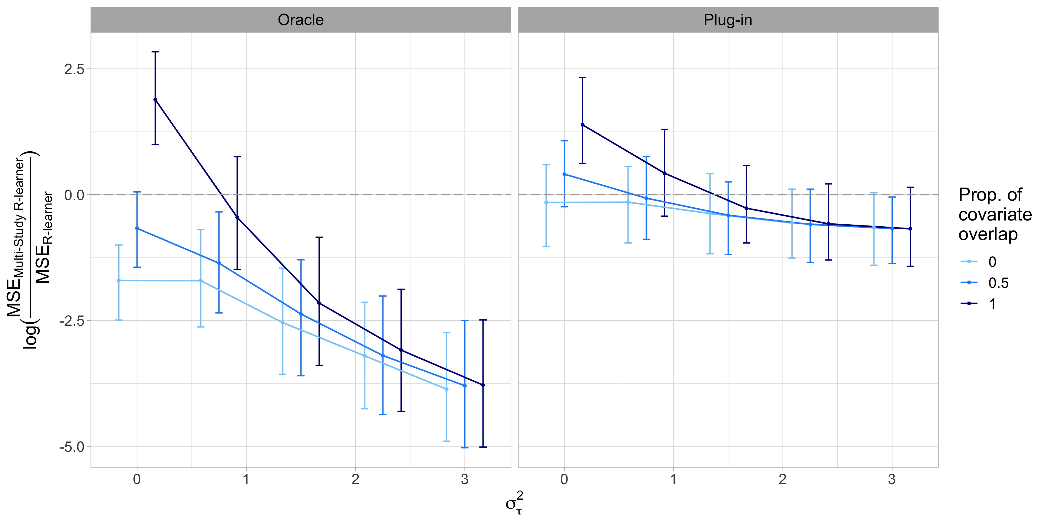
(a) Scenario C - Nonlinear treatment effect; Randomized studies

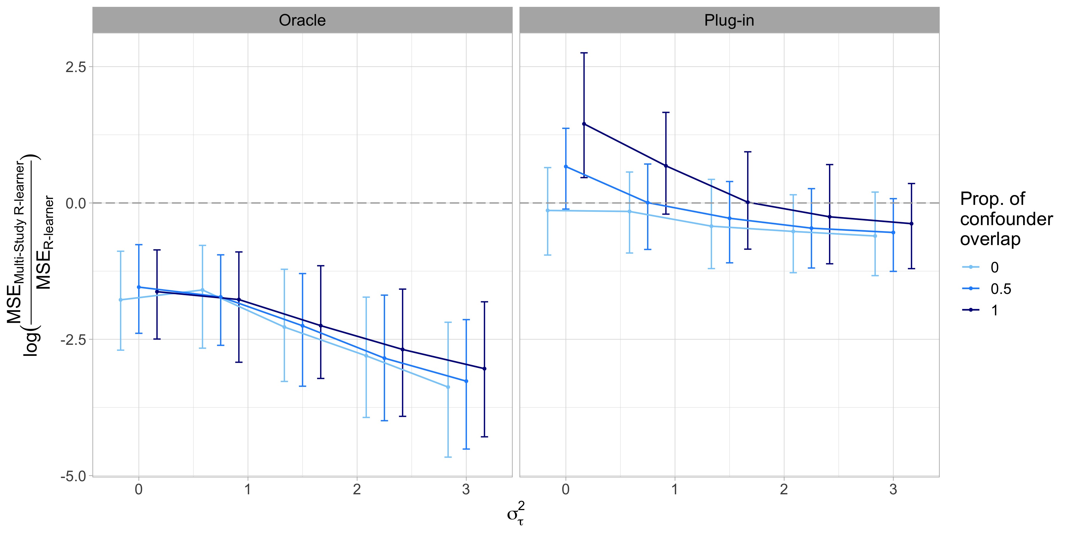
(b) Scenario D - Nonlinear treatment effect; Observational studies

Figure 2: $\log_{2}$ mean squared error (MSE) ratio comparing the multi-study $R$-learner to the $R$-learner across different levels of between-study heterogeneity. Specifically, we varied $\sigma^{2}_{\tau}$ and the proportion of covariate/confounder overlap $p_{o}$. The solid circles and vertical bars represent the average performance ratios and 95% confidence intervals, respectively, based on 500 replicates. The left panel corresponds to optimizing the oracle multi-study $R$-loss with known nuisance functions and membership probabilities, and the right panel corresponds to optimizing the plug-in multi-study $R$-loss.

Figure 2 shows the $\log_{2}$ mean squared error (MSE) ratio, i.e., $\log\left(\frac{\text{MSE}_{\text{Multi-study $R$-learner}}}{\text{MSE}_{\text{$R$-learner}}}\right)$, comparing the multi-study $R$-learner to the $R$-learner on the unseen test set. We define $\text{MSE}_{\text{model}}$ as $\frac{1}{n_{\text{test}}}\sum_{j=1}^{n_{\text{test}}}(\tau(x_{j})-\hat{\tau}_{\text{model}}(x_{j}))^{2}$, where $n_{\text{test}}$ is the number of observations in the test set. Under each scenario, we considered two optimization settings: the oracle setting where the true nuisance functions are known (left panel) and the plug-in setting where the nuisance functions need to be estimated from data (right panel). Specifically, we used elastic net to estimate the nuisance functions in the plug-in setting. Overall, as between-study heterogeneity increases, the multi-study $R$-learner outperforms the $R$-learner on the test set, and this difference in performance is more prominent in the oracle setting. When treatment is randomized (Fig. 1(a), 2(a)), merging the data and fitting an $R$-learner is preferred when between-study heterogeneity ($\sigma^{2}_{\tau}$) is low. As $\sigma^{2}_{\tau}$ increases, however, there exists a transition point beyond which the multi-study $R$-learner outperforms the $R$-learner. When studies are observational (Fig. 1(b), 2(b)), the multi-study $R$-learner shows favorable performance across all levels of $p_{o}$ and $\sigma^{2}_{\tau}$ in the oracle setting (left panel). On the other hand, the multi-study $R$-learner is preferred when between-study heterogeneity is high in the plug-in setting (right panel).

4.2 Breast Cancer Data Experiment

To illustrate the multi-study $R$-learner in a second realistic application, we used data from the curatedBreastData R package (Planey et al. (2015)). In contrast to the data experiments on ovarian cancer from the previous section, we now let both the baseline signal and the propensity scores come from real data. We considered the challenge of estimating heterogeneous treatment effects of neoadjuvant chemotherapy on breast cancer patients using randomized and observational data. Breast cancer is a molecularly heterogeneous disease consisting of four main sub-types: 1) HR+/HER2-, 2) HR-/HER2-, 3) HR+/HER2+, and 4) HR-/HER2+ (Hwang et al., 2019). HR+ means that tumor cells have excessive levels of hormone receptors (HR) for estrogen or progesterone, which promote the growth of HR+ tumors; on the other hand. HER2+ means that tumor cells produce high levels of the protein HER2 (human epidermal growth factor receptor 2), which has been shown to be associated with aggressive tumor behavior (Slamon et al. (1987)); conversely, HER2- means that tumor cells do not produce high levels of HER2. In practice, neoadjuvant chemotherapy is critical for reducing the size breast cancer before the main treatment (e.g., surgery). Because different breast cancer sub-types behave and proliferate in different ways, it’s important to characterize the heterogeneity of neoadjuvant chemotherapy, as individuals who don’t respond to chemotherapy run the additional risk of delaying surgery. Thus, the purpose of our data experiment was to characterize the heterogeneous treatment effect of anthracyline ($A$) versus taxane ($T$), two neoadjuvant chemotherapy regimens for early breast cancer.

The outcome of interest was pathological complete response, defined as disappearance of all invasive cancer in the breast after completion of neoadjuvant chemotherapy ($Y=1$) or otherwise ($Y=0$). We identified $K=2$ studies where patients were administered the neoadjuvant chemotherapy of interest. The first study (GSE21997) was a randomized trial of $n_{1}=94$ women aged between 18 and 79 with stage II-III breast cancer (Martin et al. (2011)). Patients were assigned to receive four cycles of either therapy before surgery. The second study (GSE25065) was an observational study of $n_{2}=168$ women who were HER2- with stage I-III breast cancer (Hatzis et al. (2011)). We focused on $p=105$ predictors that featured a mix of five clinical and 100 genetic covariates. The clinical covariates include age, histology grade (1-3), HR+ (1 = yes, 0 = no), PR+ (1 = yes, 0 = no), and HER2+ (1 = yes, 0 = no). In addition to these clinical features, oncologists use results from Oncotype DX, a 21-gene assay that predicts whether a patient will benefit from having chemotherapy, to help inform treatment decisions in practice (Sparano et al. (2008)). Gene expression data on eight of the 21 genes (SCUBE2, MMP11, BCL2, MYBL2, CCNB1, ACTB, TFRC, GSTM1) were available in the curatedBreastData package, and we randomly selected 92 other genes as predictors for both the treatment and outcome variables.

A challenge with illustrating heterogeneous treatment effect estimators on real data is that we do not observe both counterfactual outcomes. Therefore, we simulated study-specific treatment effects to make the task of estimating heterogeneous treatment effects non-trivial. For $k\in\{1,2\}$, $x\in\mathcal{X}$, and $i\in\{1,\ldots,n\}$, we generated

$$\tau_{k}(x)=P(Y_{i}(1)|X_{i}=x,S_{i}=k)-P(Y_{i}(0)|X_{i}=x,S_{i}=k)=:p^{(1)}_{k}(x)-p^{(0)}_{k}(x),$$

where $p^{(1)}_{k}(x)$ and $p^{(0)}_{k}(x)$ are study-specific counterfactual probabilities. We generated $p^{(1)}_{k}(x)$ and $p^{(0)}_{k}(x)$ as linear functions of the five clinical features (age, histology grade, HR+, PR+, HER2+) and eight genes (SCUBE2, MMP11, BCL2, MYBL2, CCNB1, ACTB, TFRC, GSTM1) on the logit scale. The other 92 genes were not modeled to have an effect on $p^{(1)}_{k}(x)$ and $p^{(0)}_{k}(x)$ $(k=1,2)$. Because all participants in study 2 were HER2-, we generated their counterfactual probabilities such that the HER2 effect is the same for all participants in that study. To this end, HER2 status was not a confounder in study 2. To introduce between-study heterogeneity, we assigned random effects with mean 0 and variance $\sigma^{2}_{\tau}$ to the five clinical features (age, histology grade, HR+, PR+, HER2+) and eight genes (SCUBE2, MMP11, BCL2, MYBL2, CCNB1, ACTB, TFRC, GSTM1); we varied $\sigma^{2}_{\tau}$ from 0 to 2. Details on the functional forms of $p^{(1)}_{k}(x)$ and $p^{(0)}_{k}(x)$ $(k=1,2)$ are provided in the supplement. For individuals in study $k$ with covariate $x$, we generated counterfactual outcomes $Y(a)$ from Bernoulli with probability $p^{(a)}_{k}(x)$. Finally, we set $Y=Y(a)$. We randomly divided the data into a training ($n_{\text{train}}=232$) and test set ($n_{\text{test}}=30$).

In addition to the $R$-learner, we compared our method to Wu and Yang (2021)’s integrative $R$-learner, which estimates heterogeneous treatment effects by leveraging data from a randomized controlled trial and observational study. Briefly, the integrative $R$-learner accounts for confounding bias in the observational study via the confounding function,

$$c(X)=E[Y|X,A=1,S=2]-E[Y|X,A=0,S=2]-\tau(X),$$

where $S=2$ corresponds to the observational study. This approach estimates $\tau(\cdot)$ and $c(\cdot)$ by minimizing an empirical loss function with the Neyman-orthogonal condition. To implement the $R$-learner, integrative $R$-learner, and multi-study $R$-learner, we estimated the nuisance functions from the training data using Lasso with tuning parameters selected by cross-validation. Because study 1 was a randomized trial, we used 0.5 as the propensity score, and we estimated $\hat{e}_{2}(\cdot)$ using training data from study 2. To estimate the membership probabilities for the multi-study $R$-learner, we fit a logistic regression model to the training data’s study labels, $S\in\{1,2\}$. Next, we optimized the loss functions to estimate the heterogeneous treatment effects and calculated the MSE on the test set for each approach. For the integrative $R$-learner, we used the penalty scale searching procedure to select optimal shrinkage parameters (c.f. Algorithm 1 in Wu and Yang (2021)). We applied the transformation $2\times\text{expit}(\hat{\tau}(\cdot))-1$ to ensure that $\hat{\tau}(\cdot)$ was between -1 and 1. This transformation is intuitive in that positive values of $\hat{\tau}(\cdot)$ correspond to treatment $A$ being more beneficial than $T$, and vice-versa for negative values.

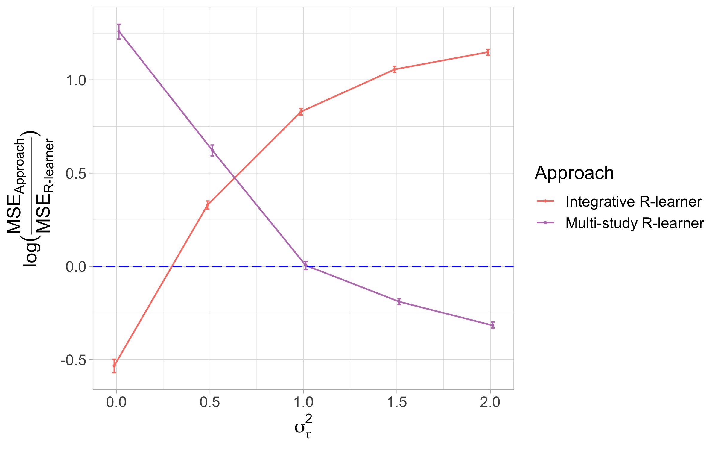
Figure 3: $\log_{2}$ mean squared error (MSE) ratio comparing the integrative $R$-learner and multi-study $R$-learner to the $R$-learner across different levels of $\sigma^{2}_{\tau}$. The solid circles and vertical bars represent the average performance ratios and 95% confidence intervals, respectively, based on 500 replicates. Red corresponds to the integrative $R$-learner and purple the multi-study $R$-learner.

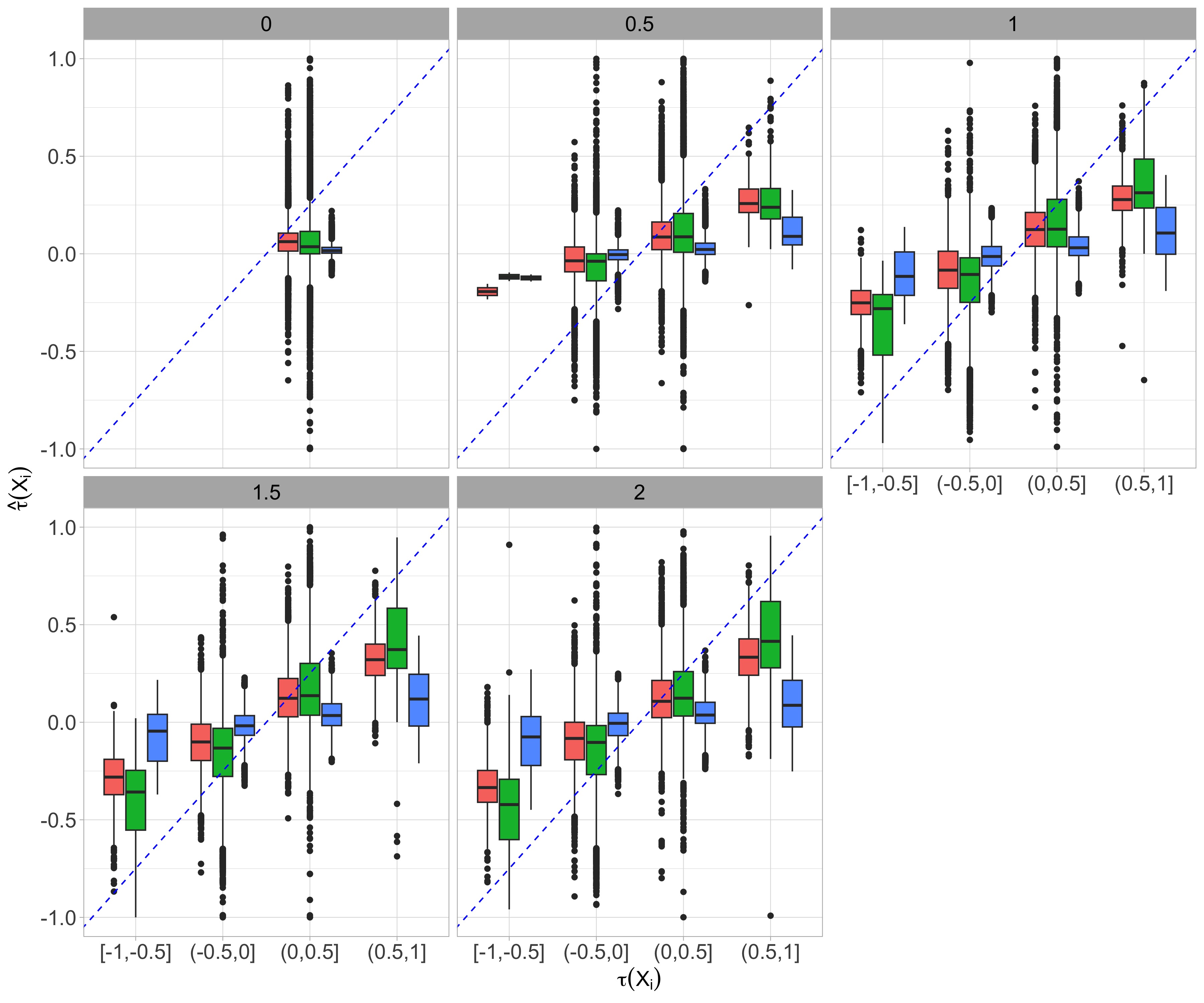
Figure 4: Estimated vs. true heterogeneous treatment effects of the $R$-learner (red), integrative $R$-learner (blue), and multi-study $R$-learner (green) across different levels of $\sigma^{2}_{\tau}$. Each panel corresponds to a specific value of $\sigma^{2}_{\tau}\in\{0,0.5,1,1.5,2\}$. The boxplots represent the distribution of $\hat{\tau}(X_{i})$ across 500 replicates.

Figure 3 shows the $\log_{2}$ MSE ratio comparing the performance of the multi-study $R$-learner and integrative $R$-learner to the original $R$-learner. Across all three methods, when there is no between-study heterogeneity $(\sigma_{\tau}=0)$, the integrative $R$-learner outperformed both the $R$-learner and the multi-study $R$-learner. As between-study heterogeneity increased, multi-study $R$-learner showed better performance compared to its counterparts. The integrative $R$-learner demonstrated the opposite trend, with worsening performance as study-level heterogeneity increased. This finding was unsurprising, as increasing the between-study heterogeneity led to the departure from the integrative $R$-learner’s transportability assumption, i.e., $\tau_{1}(x)=\tau_{2}(x)$ for all $x\in\mathcal{X}$. Figure 4 shows the true $\tau(\cdot)$ and estimated $\hat{\tau}(\cdot)$ obtained from the $R$-learner (red), multi-study $R$-learner (green), and integrative $R$-learner (blue) on the test set. Each sub-panel corresponded to the between-study heterogeneity $\sigma^{2}_{\tau}$, which ranged from 0 to 2 in increments of 0.5. When between-study heterogeneity is low, the $R$-learner has smaller bias and variance than the multi-study $R$-learner. As between-study heterogeneity increased, bias increased; in particular, the $R$-learner tended to have larger bias at more extreme values of $\tau(X_{i})$ (i.e., $\tau(X_{i})\in[-1,-0.5]$ and $\tau(X_{i})\in(0.5,1]$) than the multi-study $R$-learner. Thus, when $\sigma^{2}_{\tau}$ was high (e.g., $\sigma^{2}_{\tau}>1$), the multi-study $R$-learner had smaller estimation error compared to the $R$-learner (Figure 3). The integrative $R$-learner had higher MSE than its counterparts when $\sigma^{2}_{\tau}$ was relatively low, suggesting that it was sensitive to even small departures from the transportability assumption.

5 Discussion

In this work, we proposed the multi-study $R$-learner for estimating heterogeneous treatment effects in the presence of between-study heterogeneity. By leveraging cross-study estimates of nuisance functions and heterogeneous treatment effects via membership probabilities, the multi-study $R$-learner is able to borrow strength across potentially heterogeneous studies. The structure of the multi-study $R$-loss not only eliminates spurious effects between nuisance functions, making the resulting estimator robust to between-study heterogeneity in confounding adjustment, but also enables us to estimate the causal effect of interest accurately in terms of empirical performance and asymptotic guarantees. In the presence of between-study heterogeneity, our approach showed preferable performance over the $R$-learner and integrative $R$-learner. The latter is the only other multi-study variant of the $R$-learner that we know of. The integrative $R$-learner was developed for the setting where $K=2$ studies have identical heterogeneous treatment effects. In comparison, the multi-study $R$-learner is more flexible, as it can be broadly applied to $K>2$ studies that have between-study heterogeneity in the treatment effects.

Our proposed framework provides considerable flexibility for multi-study learning. For example, the choice of merging vs. study-specific learning for the mean outcome model may impact the estimation of heterogeneous treatment effects. The former refers to pooling all studies and training a single model, and the latter training a separate model on each study and ensembling the resulting predictions. When studies are relatively homogeneous, Patil and Parmigiani (2018) showed that merging can lead to improved performance over ensembling due to increase in sample size; as between-study heterogeneity increases, multi-study ensembling is preferred. The trade-off between merging and multi-study ensembling has been explored in detail for ML techniques, including linear regression (Guan et al. (2019)), random forest (Ramchandran et al. (2020)), and gradient boosting (Shyr et al. (2022)). Ren et al. (2020) explored cross-validation approaches for multi-study stacking, an ensemble learning approach where each ML model is weighted by their ability to make cross-study replicable predictions. While we estimated the mean outcome function via a pooled analysis of the $K$ studies, an alternative strategy is to estimate study-specific functions and combine them using membership probabilities. As such, an interesting generalization of the current work is to explore different cross-study ML strategies, such as model stacking (Breiman, 1996), when estimating the mean outcome function.

We draw parallels between the multi-study $R$-learner and several related lines of work. The first is federated learning across distributed data networks. In this setting, information exchange between data sites may be restricted due to privacy or feasibility considerations, prohibiting pooled analyses (Maro et al., 2009; McMahan et al., 2017). As such, study sites leverage models or parameters derived from other sites without sharing individual-level data. In the context of heterogeneous treatment effect estimation, Tan et al. (2022) proposed a tree-based ensemble approach that combines models across data sites. Vo et al. (2022) performed federated causal inference through adaptive kernel functions on observational studies. Similar to this line of work, the multi-study $R$-learner performs cross-site learning by computing study-specific nuisance functions and heterogeneous treatment effects for all individuals. Currently, our approach requires centralized access to individual-level data from all sites, and, as a result, is not directly applicable to distributed data. Adapting the multi-study $R$-learner to the federated setting would require the addition of a transportability (or partial transportability) assumption, i.e., $\{Y(1),Y(0)\}\perp\!\!\!\perp S|X$, and the new loss function cannot be interpreted as easily. Thus, we leave this extension to future work.

Another related line of work is transporting causal effects to a target population by leveraging data from source studies. This has been explored in detail for average treatment effects (Buchanan et al., 2018; Dahabreh et al., 2019; Dahabreh and Hernán, 2019) and heterogeneous treatment effects (Wu and Yang, 2021; Kallus et al., 2018; Cheng and Cai, 2021; Hatt et al., 2022). Similar to this line of work, the multi-study $R$-learner estimates treatment effect in a target population by leveraging information from $K$ source studies through membership probabilities, which reflect how similar individuals in the target population are to those in the source studies. Specifically, the target population consists of new individuals from whom we don’t observe the study label $S$ or treatment assignment $A$. In precision medicine, these individuals represent patients for whom the clinician will tailor the treatment regime based on their covariates. In contrast to this line of work, the multi-study $R$-learner is more general because it does not assume identical treatment effects across all or a subset of source studies. Domain adaption or transfer learning on heterogeneous feature spaces is another related avenue to our work (Johansson et al., 2018; Shi et al., 2021). Recently, Bica and van der Schaar (2022) used representation learning to transfer heterogeneous treatment effects across different feature spaces. Specifically, the authors’ approach to domain-specific and shared confounders is pertinent and can be incorporated into the multi-study $R$-learner framework as an extension of the current work.

In many areas of research, facilitation of systematic data-sharing increased access to multiple studies that target the same treatment. While this offers new opportunities for estimating treatment effects, it is critical to simultaneously consider and systematically integrate multiple studies in the presence of between-study heterogeneity.

6 Funding

This work was supported by the NIH grant 5T32CA009337-40 (Shyr) and NSF-DMS 2113707 (Parmigiani and Ren).

7 Data availability and code

Data and code to reproduce results from this paper can be found at
https://github.com/cathyshyr/multi-study-r-learner.

8 Figures

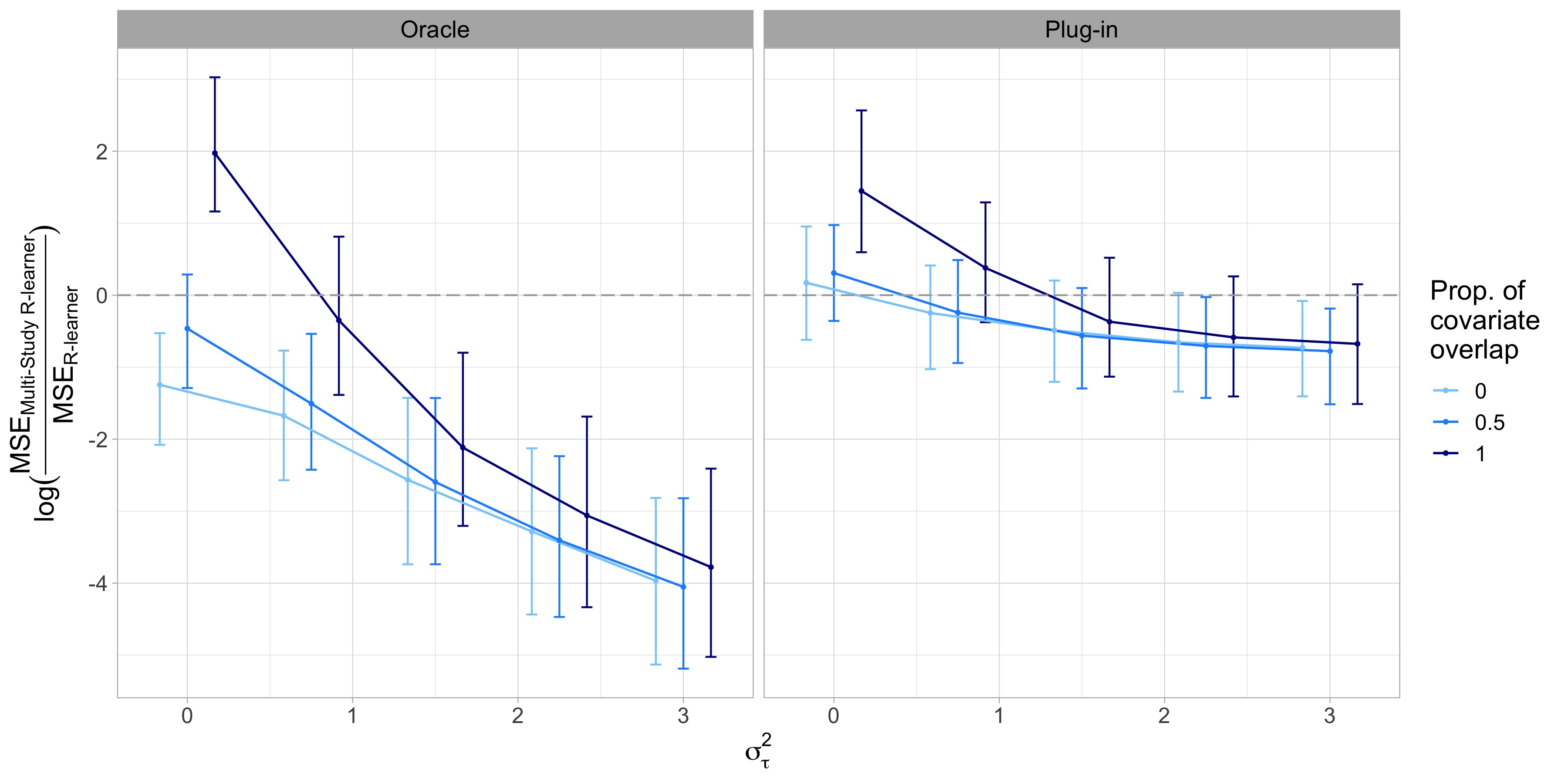
(a) Scenario A - Linear treatment effect; Randomized studies

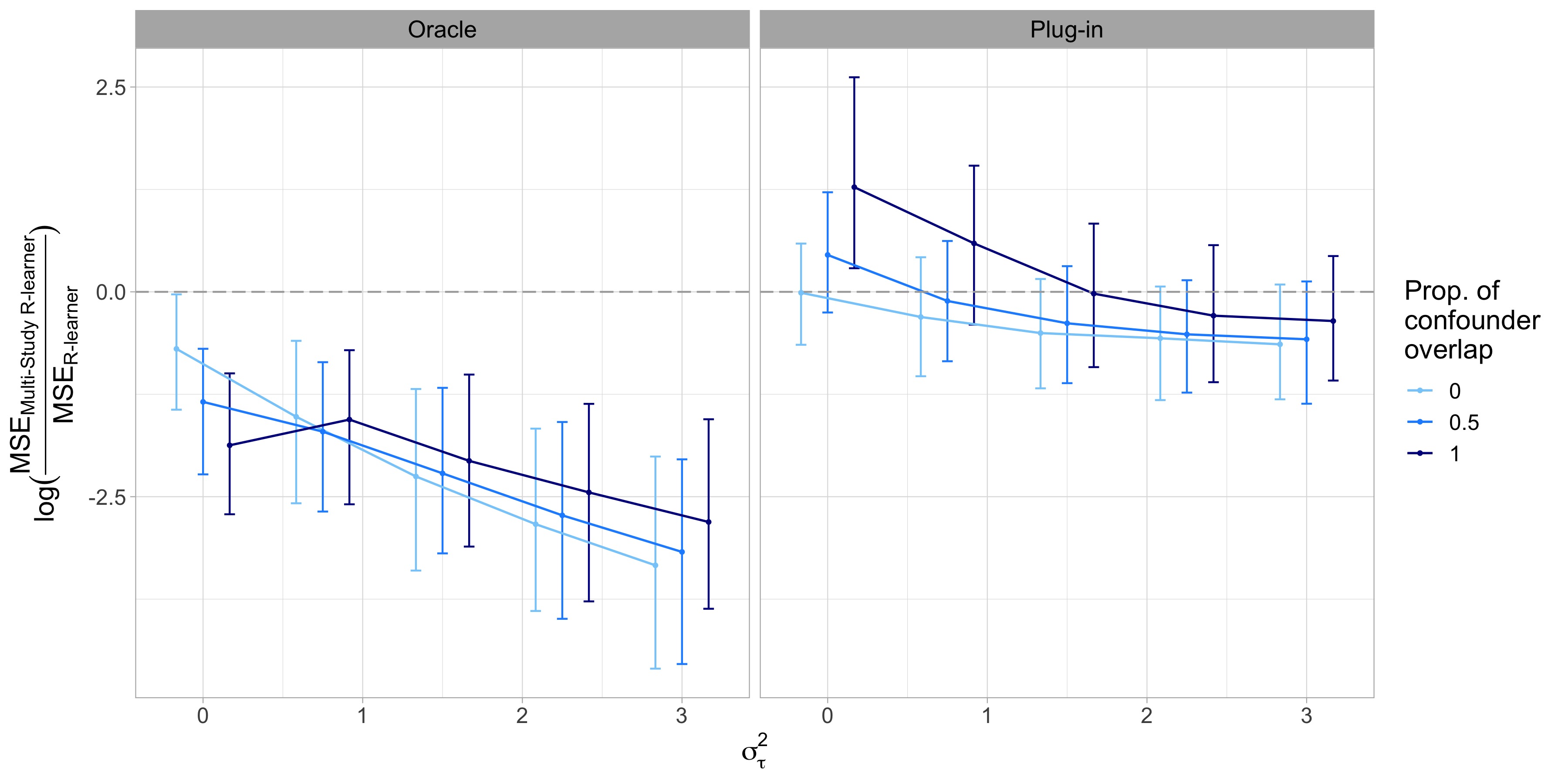
(b) Scenario B - Linear treatment effect; Observational studies

9 Supplement

9.1 Simulation parameters for the membership probability

$$X_{i}\beta_{2} =-0.841+1.384X_{i1}-0.158X_{i13}-1.072X_{i14}+1.499X_{i27}$$

$$\quad-1.010X_{i36}-2X_{i37}-0.143X_{i39}+1.55X_{i40}$$

$$X_{i}\beta_{3} =-0.113+0.233X_{i2}-1.272X_{i11}-0.205X_{i13}+0.347X_{i15}$$

$$\quad+0.0323X_{i16}+0.121X_{i20}+0.926X_{i33}-1.062X_{i34}$$

$$X_{i}\beta_{4} =-1.351-0.202X_{i5}+1.059X_{i10}+1.243X_{i13}+0.732X_{i20}$$

$$\quad+0.456X_{i21}+0.648X_{i24}-0.392X_{i35}+0.752X_{i37}.$$

9.2 Parameters for the breast cancer data experiment

Let $\gamma^{(1)}_{k,j},\gamma^{(0)}_{k,j}\sim N(0,\sigma^{2}_{\tau})$ denote the random effects associated with the $j$th covariate in study $k$ for counterfactual outcomes when $A=1$ and $A=0$, respectively.

$$p^{(1)}_{1}(x)=expit( (-0.28-0.087\cdot\text{age}+(0.077+\gamma^{(1)}_{1,1})\cdot I(\text{ER+}=1)-(0.34+\gamma^{(1)}_{1,2})\cdot I(\text{PR+}=1)$$

$$+(0.058+\gamma^{(1)}_{1,3})\cdot I(\text{HER2+}=1)+(0.009+\gamma^{(1)}_{1,4})\cdot\text{histology}+(0.025+\gamma^{(1)}_{1,5})\cdot\textit{SCUBE2}$$

$$+(0.33+\gamma^{(1)}_{1,6})\cdot\textit{MMP11}-(0.36+\gamma^{(1)}_{1,7})\cdot\textit{BCL2}+(0.38+\gamma^{(1)}_{1,8})\cdot\textit{MYBL2}$$

$$-(0.22+\gamma^{(1)}_{1,9})\cdot\textit{CCNB1}-(0.33+\gamma^{(1)}_{1,10})\cdot\textit{ACTB}-(0.21+\gamma^{(1)}_{1,11})\cdot\textit{TFRC}$$

$$+(0.075+\gamma^{(1)}_{1,12})\cdot\textit{GSTM1})/50)$$

$$p^{(0)}_{1}(x)=expit( (0.062-0.56\cdot\text{age}-(0.20+\gamma^{(0)}_{1,1})\cdot I(\text{ER+}=1)+(0.14+\gamma^{(0)}_{1,2})\cdot I(\text{PR+}=1)$$

$$(-0.13+\gamma^{(0)}_{1,3})\cdot I(\text{HER2+}=1)-(0.083+\gamma^{(0)}_{1,4})\cdot\text{histology}-(0.12+\gamma^{(0)}_{1,5})\cdot\textit{SCUBE2}$$

$$+(0.48+\gamma^{(0)}_{1,6})\cdot\textit{MMP11}-(0.21+\gamma^{(0)}_{1,7})\cdot\textit{BCL2}-(0.13+\gamma^{(0)}_{1,8})\cdot\textit{MYBL2}$$

$$+(0.004+\gamma^{(0)}_{1,9})\cdot\textit{CCNB1}+(0.064+\gamma^{(0)}_{1,10})\cdot\textit{ACTB}+(0.056+\gamma^{(0)}_{1,11})\cdot\textit{TFRC}$$

$$-(0.015+\gamma^{(0)}_{1,12})\cdot\textit{GSTM1})/50)$$

$$p^{(1)}_{2}(x)=expit( (-0.28-0.087\cdot\text{age}+(0.077+\gamma^{(1)}_{2,1})\cdot I(\text{ER+}=1)-(0.34+\gamma^{(1)}_{2,2})\cdot I(\text{PR+}=1)$$

$$+(0.009+\gamma^{(1)}_{2,3})\cdot\text{histology}+(0.025+\gamma^{(1)}_{2,4})\cdot\textit{SCUBE2}+(0.33+\gamma^{(1)}_{2,5})\cdot\textit{MMP11}$$

$$-(0.36+\gamma^{(1)}_{2,6})\cdot\textit{BCL2}+(0.38+\gamma^{(1)}_{2,7})\cdot\textit{MYBL2}-(0.22+\gamma^{(1)}_{2,8})\cdot\textit{CCNB1}$$

$$-(0.33+\gamma^{(1)}_{2,9})\cdot\textit{ACTB}-(0.21+\gamma^{(1)}_{2,10})\cdot\textit{TFRC}+(0.075+\gamma^{(1)}_{2,11})\cdot\textit{GSTM1})/50)$$

$$p^{(0)}_{2}(x)=expit( (0.062-0.56\cdot\text{age}-(0.20+\gamma^{(0)}_{2,1})\cdot I(\text{ER+}=1)+(0.14+\gamma^{(0)}_{2,2})\cdot I(\text{PR+}=1)$$

$$-(0.083+\gamma^{(0)}_{2,3})\cdot\text{histology}-(0.12+\gamma^{(0)}_{2,4})\cdot\textit{SCUBE2}+(0.48+\gamma^{(0)}_{2,5})\cdot\textit{MMP11}$$

$$-(0.21+\gamma^{(0)}_{2,6})\cdot\textit{BCL2}-(0.13+\gamma^{(0)}_{2,7})\cdot\textit{MYBL2}+(0.004+\gamma^{(0)}_{2,8})\cdot\textit{CCNB1}$$

$$+(0.064+\gamma^{(0)}_{2,9})\cdot\textit{ACTB}+(0.056+\gamma^{(0)}_{2,10})\cdot\textit{TFRC}-(0.015+\gamma^{(0)}_{2,11})\cdot\textit{GSTM1})/50)$$

9.3 Proofs

Proof 9.2 (Proposition 1).

$$E[\epsilon_{i}|X_{i},A_{i}]= E[Y_{i}(A_{i})|A_{i},X_{i}]-E\left[\left.\sum_{k=1}^{K}\left\{\mu_{k}^{(0)}(X_{i})+A_{i}\tau_{k}(X_{i})\right\}p(k|X_{i})\right|A_{i},X_{i}\right]$$

$$= E[Y_{i}(A_{i})|A_{i},X_{i}]-\sum_{k=1}^{K}p(k|X_{i})E[\underbrace{E[Y_{i}(0)|X_{i},S_{i}=k]}_{\mu_{k}^{(0)}(X_{i})}|A_{i},X_{i}]$$

$$-A_{i}\sum_{k=1}^{K}p(k|X_{i})E[\underbrace{E[Y_{i}(1)-Y_{i}(0)|X_{i},S_{i}=k]}_{\tau_{k}(X_{i})}|A_{i},X_{i}]$$

$$= E[Y_{i}(A_{i})|A_{i},X_{i}]-(1-A_{i})\sum_{k=1}^{K}p(k|X_{i})E[E[Y_{i}(0)|X_{i},S_{i}=k]|A_{i},X_{i}]$$

$$-A_{i}\sum_{k=1}^{K}p(k|X_{i})E[E[Y_{i}(1)|X_{i},S_{i}=k]|A_{i},X_{i}]$$

$$= E[Y_{i}(A_{i})|A_{i},X_{i}]-(1-A_{i})\sum_{k=1}^{K}p(k|X_{i})E[E[Y_{i}(0)|A_{i}=0,X_{i},S_{i}=k]|A_{i},X_{i}]$$

$$-A_{i}\sum_{k=1}^{K}p(k|X_{i})E[E[Y_{i}(1)|A_{i}=1,X_{i},S_{i}=k]|A_{i},X_{i}]$$

$$= 0$$

The second to last equality holds by Assumption 2. The last equality holds because for $A_{i}=a\in\{0,1\}$, we have

$$E[Y_{i}(a)|A_{i}=a,X_{i}]-\sum_{k=1}^{K}p(k|X_{i})E[E[Y_{i}(a)|A_{i}=a,X_{i},S_{i}=k]|A_{i}=a,X_{i}]$$

$$= E[Y_{i}(a)|A_{i}=a,X_{i}]-\sum_{k=1}^{K}p(k|X_{i})E[Y_{i}(a)|A_{i}=a,X_{i}]$$

$$= E[Y_{i}(a)|A_{i}=a,X_{i}]-E[Y_{i}(a)|A_{i}=a,X_{i}]$$

$$= 0.$$

Proof 9.3 (Lemma 1).

Recall that

$$\hat{L}_{n}(\beta)=\frac{1}{n}\sum_{i=1}^{n}\left[\{Y_{i}-\hat{m}^{-q(i)}(X_{i})\}-\hat{u}_{i}^{\intercal}\beta\right]^{2}$$

and

$$L_{n}(\beta)=\frac{1}{n}\sum_{i=1}^{n}\left[\{Y_{i}-{m}(X_{i})\}-u_{i}^{\intercal}\beta\right]^{2}.$$

We can re-write $\hat{L}_{n}(\beta)$ as

$$\hat{L}_{n}(\beta)=\frac{1}{n}\sum_{i=1}^{n}\left[\{Y_{i}-\hat{m}^{-q(i)}(X_{i})\}-\sum_{k=1}^{K}\{A_{i}-\hat{e}^{-q_{k}(i)}_{k}(X_{i})\}\hat{p}^{-q(i)}(k|X_{i})v_{k}(X_{i})^{\intercal}\beta_{k}\right]^{2},$$

where $\beta_{k}\in\mathbb{R}^{d_{k}}$ is the vector of coefficients for study $k$. Similarly, we can re-write $L_{n}(\beta)$ as

$$L_{n}(\beta)=\frac{1}{n}\sum_{i=1}^{n}\left[\{Y_{i}-m(X_{i})\}-\sum_{k=1}^{K}\{A_{i}-e_{k}(X_{i})\}p(k|X_{i})v_{k}(X_{i})^{\intercal}\beta_{k}\right]^{2}.$$

We define the following notation:

$$A_{m,i} =m(X_{i})-\hat{m}^{-q(i)}(X_{i})$$

$$A_{e_{k},i} =(e_{k}(X_{i})-A_{i})p(k|X_{i})-(\hat{e}^{-q_{k}(i)}_{k}(X_{i})-A_{i})\hat{p}^{-q(i)}(k|X_{i})\hskip 30.00005ptk=1,\ldots,K$$

$$B_{m,i} =Y_{i}-m(X_{i})$$

$$B_{e_{k},i} =(A_{i}-e_{k}(X_{i}))p(k|X_{i})\hskip 30.00005ptk=1,\ldots,K$$

$$g_{k}(X_{i},\beta_{k}) =v_{k}(X_{i})^{\intercal}\beta_{k}$$

$$A_{e,i} =\sum_{k=1}^{K}A_{e_{k},i}g_{k}(X_{i};\beta_{k})$$

$$B_{e,i} =\sum_{k=1}^{K}B_{e_{k},i}g_{k}(X_{i};\beta_{k}),$$

By algebra, we have

$$\hat{L}_{n}(\beta)= \frac{1}{n}\sum_{i=1}^{n}\left[B_{m,i}+A_{m,i}-\sum_{k=1}^{K}(B_{e_{k},i}+A_{e_{k},i})g_{k}(X_{i};\beta_{k})\right]^{2}$$

$$= \frac{1}{n}\sum_{i=1}^{n}\left[B_{m,i}+A_{m,i}-B_{e,i}-A_{e,i}\right]^{2}$$

$$= L_{n}(\beta)+\frac{1}{n}\sum_{i=1}^{n}\left[A_{m,i}-A_{e,i}\right]^{2}+\frac{2}{n}\sum_{i=1}^{n}(B_{m,i}-B_{e,i})(A_{m,i}-A_{e,i})$$

$$= L_{n}(\beta)+\frac{1}{n}\sum_{i=1}^{n}A^{2}_{m,i}+\frac{1}{n}\sum_{i=1}^{n}A_{e,i}^{2}-\frac{2}{n}\sum_{i=1}^{n}A_{m,i}A_{e,i}$$

$$+\frac{2}{n}\sum_{i=1}^{n}B_{m,i}A_{m,i}-\frac{2}{n}\sum_{i=1}^{n}B_{m,i}A_{e,i}-\frac{2}{n}\sum_{i=1}^{n}B_{e,i}A_{m,i}+\frac{2}{n}\sum_{i=1}^{n}B_{e,i}A_{e,i}$$

First term: $\frac{1}{n}\sum_{i=1}^{n}A^{2}_{m,i}=\frac{1}{n}\sum_{i=1}^{n}(m(X_{i})-\hat{m}^{-q(i)}(X_{i}))^{2}$

By Markov’s inequality and Assumption 5, $\frac{1}{n}\sum_{i=1}^{n}A^{2}_{m,i}$ is $O_{p}(a^{2}_{n}).$

Second term: $\frac{1}{n}\sum_{i=1}^{n}A^{2}_{e,i}=\frac{1}{n}\sum_{i=1}^{n}\left[\sum_{k=1}^{K}A_{e_{k},i}g_{k}(X_{i};\beta_{k})\right]^{2}$

We have

$$\frac{1}{n}\sum_{i=1}^{n}A^{2}_{e,i} =\sum_{k=1}^{K}\left[\frac{1}{n}\sum_{i=1}^{n}\left\{(e_{k}(X_{i})-A_{i})p(k|X_{i})-(\hat{e}^{-q_{k}(i)}_{k}(X_{i})-A_{i})\hat{p}^{-q(i)}(k|X_{i})\right\}^{2}g_{k}(X_{i};\beta_{k})^{2}\right]$$

$$\quad+\sum_{k\neq k^{\prime}}\left[\frac{2}{n}\sum_{i=1}^{n}\left\{(e_{k}(X_{i})-A_{i})p(k|X_{i})-(\hat{e}^{-q_{k}(i)}_{k}(X_{i})-A_{i})\hat{p}^{-q(i)}(k|X_{i})\right\}g_{k}(X_{i};\beta_{k})\right.$$

$$\hskip 44.10011pt\left.\times\left\{(e_{k^{\prime}}(X_{i})-A_{i})p(k^{\prime}|X_{i})-(\hat{e}^{-q_{k}(i)}_{k^{\prime}}(X_{i})-A_{i})\hat{p}^{-q(i)}(k^{\prime}|X_{i})\right\}g_{k^{\prime}}(X_{i};\beta_{k^{\prime}})\right]$$

By Markov’s inequality and Assumption 5, the first sum is $O_{p}(a^{2}_{n}).$ Similarly, the cross term is also $O_{p}(a^{2}_{n}).$ Therefore, we can conclude that $\frac{1}{n}\sum_{i=1}^{n}A^{2}_{e,i}$ is $O_{p}(a^{2}_{n}).$

Third term: $\frac{1}{n}\sum_{i=1}^{n}A_{m,i}A_{e,i}$

We have

$$\frac{1}{n}\sum_{i=1}^{n}A_{m,i}A_{e,i} =\frac{1}{n}\sum_{i=1}^{n}\left\{(m(X_{i})-\hat{m}^{-q(i)}(X_{i}))\left[\sum_{k=1}^{K}\left\{(e_{k}(X_{i})-A_{i})p(k|X_{i})-(\hat{e}^{-q_{k}(i)}_{k}(X_{i})-A_{i})\hat{p}^{-q(i)}(k|X_{i})\right\}g_{k}(X_{i};\beta_{k})\right]\right\}$$

$$\leq\frac{C_{1}}{n}\sum_{i=1}^{n}\left\{(m(X_{i})-\hat{m}^{-q(i)}(X_{i}))\left[\sum_{k=1}^{K}(e_{k}(X_{i})-A_{i})p(k|X_{i})-(\hat{e}^{-q_{k}(i)}_{k}(X_{i})-A_{i})\hat{p}^{-q(i)}(k|X_{i})\right]\right\}$$

$$\leq C_{1}\sqrt{\left(\frac{1}{n}\sum_{i=1}^{n}\left\{m(X_{i})-\hat{m}^{-q(i)}(X_{i})\right\}^{2}\right)\left\{\frac{1}{n}\sum_{i=1}^{n}\left[\sum_{k=1}^{K}(e_{k}(X_{i})-A_{i})p(k|X_{i})-(\hat{e}^{-q_{k}(i)}_{k}(X_{i})-A_{i})\hat{p}^{-q(i)}(k|X_{i})\right]^{2}\right\}}$$

$$=O_{p}(a^{2}_{n})$$

for some constant $C_{1}$. The second line holds by Assumption 4, and the third line holds by Cauchy-Schwarz inequality.

Fourth term: $\frac{1}{n}\sum_{i=1}^{n}B_{m,i}A_{m,i}=\frac{1}{n}\sum_{i=1}^{n}(Y_{i}-m(X_{i}))(m(X_{i})-\hat{m}^{-q(i)}(X_{i}))$

We define

$$B^{q}_{mm}=\frac{1}{|\{i:q(i)=q\}|}\sum_{i:q(i)=q}B_{m,i}A_{m,i}$$

to be the sample average of $B_{m,i}A_{m,i}$ in the $q$th cross-fitting fold. By the triangle inequality,

$$\left|\frac{1}{n}\sum_{i=1}^{n}(Y_{i}-m(X_{i}))(m(X_{i})-\hat{m}^{-q(i)}(X_{i}))\right|\leq\sum_{q=1}^{Q}|B^{q}_{mm}|.$$

Therefore, it suffices to show that $B^{q}_{mm}=O_{p}(a^{2}_{n}).$ Let $\mathcal{I}^{-q}=\{X_{i},A_{i},Y_{i},S_{i}:q(i)\neq q\}$ denote the set of observations that do not belong to the same data fold as observation $i.$ $B^{q}_{mm}$’s expectation is

$$E\left(B^{q}_{mm}\right) =E(B_{m,i}A_{m,i})$$

$$=E\left(E\left[B_{m,i}A_{m,i}|\mathcal{I}^{-q},X_{i}\right]\right)$$

$$=E(A_{m,i}E\left[B_{m,i}|\mathcal{I}^{-q},X_{i}\right])$$

$$=0,$$

where the last line follows from Assumption 1 and Assumption 2.

Next, its variance is

$$Var\left(B_{mm}^{q}\right) =E\left\{\left(B_{mm}^{q}\right)^{2}\right\}$$

$$=\frac{E\left\{\sum_{i:q(i)=q}B_{m,i}^{2}A_{m,i}^{2}+\sum_{i\neq j:q(i)=q,q(j)=q}B_{m,i}B_{m,j}A_{m,i}A_{m,j}\right\}}{|\{i:q(i)=q\}|^{2}}$$

$$=\frac{E\left(B_{m,i}^{2}A_{m,i}^{2}\right)}{|\{i:q(i)=q\}|}+\frac{\sum_{i\neq j:q(i)=q,q(j)=q}E\left(B_{m,i}B_{m,j}A_{m,i}A_{m,j}\right)}{|\{i:q(i)=q\}|^{2}}$$

For the first term, we have

$$E\left(B_{m,i}^{2}A_{m,i}^{2}\right) =E\left(E\left[B_{m,i}^{2}A_{m,i}^{2}|\mathcal{I}^{-q},X_{i}\right]\right)$$

$$=E\left(A_{m,i}^{2}E\left[B_{m,i}^{2}|\mathcal{I}^{-q},X_{i}\right]\right)$$

$$\leq C_{2}E(A_{m,i}^{2})$$

$$=O(a^{2}_{n})$$

for some constant $C_{2}.$ The second to last line holds from Assumption 4. And the last line holds from Assumption 5.

For the second term, we have

$$E\left(B_{m,i}B_{m,j}A_{m,i}A_{m,j}\right) =E\left[E\left(B_{m,i}B_{m,j}A_{m,i}A_{m,j}|\mathcal{I}^{-q},X_{i}\right)\right]$$

$$=E\left[A_{m,i}A_{m,j}E\left(B_{m,i}B_{m,j}|\mathcal{I}^{-q},X_{i}\right)\right]$$

$$=E\left[A_{m,i}A_{m,j}E\left(B_{m,j}|\mathcal{I}^{-q},X_{i}\right)E\left(B_{m,i}|\mathcal{I}^{-q},X_{i}\right)\right]$$

$$=0$$

The second to last line follows because $B_{m,i}$ is independent of $B_{m,j}$ for $i\neq j$. The last line follows by the definition of $B_{m,i}$. Therefore, we have that

$$Var(B^{q}_{mm})=\frac{Q}{n}O(a^{2}_{n})=O({a^{2}_{n}}/n),$$

where the first equality holds if the $Q$ folds have equal number of observations (i.e., $n/Q$ for each fold). Then by Chebychev’s inequality, $\frac{1}{n}\sum_{i=1}^{n}B_{m,i}A_{m,i}=O_{p}(a^{2}_{n}/n).$

Fifth term:

$$\frac{1}{n}\sum_{i=1}^{n}B_{m,i}A_{e,i}$$

$$= \frac{1}{n}\sum_{i=1}^{n}\left[(Y_{i}-m(X_{i}))\left\{\sum_{k=1}^{K}\left\{(e_{k}(X_{i})-A_{i})p(k|X_{i})-(\hat{e}^{-q_{k}(i)}_{k}(X_{i})-A_{i})\hat{p}^{-q(i)}(k|X_{i})\right\}g_{k}(X_{i};\beta_{k})\right\}\right]$$

We define

$$B^{q}_{me}=\frac{1}{|\{i:q(i)=q\}|}\sum_{i:q(i)=q}B_{m,i}A_{e,i}$$

to be the sample average of $B_{m,i}A_{e,i}$ in the $q$th cross-fitting fold. By the triangle inequality,

$$\left|\frac{1}{n}\sum_{i=1}^{n}\left[(Y_{i}-m(X_{i}))\left\{\sum_{k=1}^{K}\left\{(e_{k}(X_{i})-A_{i})p(k|X_{i})-(\hat{e}^{-q_{k}(i)}_{k}(X_{i})-A_{i})\hat{p}^{-q(i)}(k|X_{i})\right\}g_{k}(X_{i};\beta_{k})\right\}\right]\right|\leq\sum_{q=1}^{Q}|B^{q}_{me}|.$$

Therefore, it suffices to show that $B^{q}_{me}=O_{p}(a^{2}_{n}).$ Its expectation is

$$E\left(B^{q}_{me}\right) =E(B_{m,i}A_{e,i})$$

$$=E\left(E\left[B_{m,i}A_{e,i}|\mathcal{I}^{-q},X_{i},A_{i}\right]\right)$$

$$=E(A_{e,i}E\left[B_{m,i}|\mathcal{I}^{-q},X_{i},A_{i}\right])$$

$$=0,$$

where the last line follows from the definition of $B_{m,i}.$

Next, its variance is

$$Var\left(B_{me}^{q}\right) =E\left\{\left(B_{me}^{q}\right)^{2}\right\}$$

$$=\frac{E\left\{\sum_{i:q(i)=q}B_{m,i}^{2}A_{e,i}^{2}+\sum_{i\neq j:q(i)=q,q(j)=q}B_{m,i}B_{m,j}A_{e,i}A_{e,j}\right\}}{|\{i:q(i)=q\}|^{2}}$$

$$=\frac{E\left(B_{m,i}^{2}A_{e,i}^{2}\right)}{|\{i:q(i)=q\}|}+\frac{\sum_{i\neq j:q(i)=q,q(j)=q}E\left(B_{m,i}B_{m,j}A_{e,i}A_{e,j}\right)}{|\{i:q(i)=q\}|^{2}}$$

For the first term, we have

$$E\left(B_{m,i}^{2}A_{e,i}^{2}\right) =E\left(E\left[B_{m,i}^{2}A_{e,i}^{2}|\mathcal{I}^{-q},X_{i},A_{i}\right]\right)$$

$$=E\left(A_{e,i}^{2}E\left[B_{m,i}^{2}|\mathcal{I}^{-q},X_{i},A_{i}\right]\right)$$

$$\leq C_{2}E(A_{e,i}^{2})$$

$$=O(a^{2}_{n})$$

for some constant $C_{2}.$ The second to last line holds from Assumption 4. And the last line holds from Assumption 5.

For the second term, we have

$$E\left(B_{m,i}B_{m,j}A_{e,i}A_{e,j}\right) =E\left[E\left(B_{m,i}B_{m,j}A_{e,i}A_{e,j}|\mathcal{I}^{-q},X_{i},A_{i}\right)\right]$$

$$=E\left[A_{e,i}A_{e,j}E\left(B_{m,i}B_{m,j}|\mathcal{I}^{-q},X_{i},A_{i}\right)\right]$$

$$=E\left[A_{e,i}A_{e,j}E\left(B_{m,j}|\mathcal{I}^{-q},X_{i},A_{i}\right)E\left(B_{m,i}|\mathcal{I}^{-q},X_{i},A_{i}\right)\right]$$

$$=0$$

The second to last line follows because $B_{m,i}$ is independent of $B_{m,j}$ for $i\neq j$. The last line follows the definition of $B_{m,i}$. Therefore, we have that

$$Var(B^{q}_{me})=\frac{Q}{n}O(a^{2}_{n})=O({a^{2}_{n}}/n),$$

where the first equality holds if the $Q$ folds have equal number of observations (i.e., $n/Q$ for each fold). Then by Chebychev’s inequality, $\frac{1}{n}\sum_{i=1}^{n}B_{m,i}A_{e,i}=O_{p}(a^{2}_{n}/n).$

Sixth term:

$$\frac{1}{n}\sum_{i=1}^{n}B_{e,i}A_{m,i}$$

$$= \frac{1}{n}\sum_{i=1}^{n}\left[\left\{\sum_{k=1}^{K}(A_{i}-e_{k}(X_{i}))p(k|X_{i})g_{k}(X_{i};\beta_{k})\right\}(m(X_{i})-\hat{m}^{-q(i)}(X_{i}))\right]$$

We define

$$B^{q}_{em}=\frac{1}{|\{i:q(i)=q\}|}\sum_{i:q(i)=q}B_{e,i}A_{m,i}$$

to be the sample average of $B_{e,i}A_{m,i}$ in the $q$th cross-fitting fold. By the triangle inequality,

$$\left|\frac{1}{n}\sum_{i=1}^{n}\left[\left\{\sum_{k=1}^{K}(A_{i}-e_{k}(X_{i}))p(k|X_{i})g_{k}(X_{i};\beta_{k})\right\}(m(X_{i})-\hat{m}^{-q(i)}(X_{i}))\right]\right|\leq\sum_{q=1}^{Q}|B^{q}_{em}|.$$

Therefore, it suffices to show that $B^{q}_{em}=O_{p}(a^{2}_{n}).$ Its expectation is

$$E(B^{q}_{em}) =E(B_{e,i}A_{m,i})$$

$$=E(E\left[B_{e,i}A_{m,i}|\mathcal{I}^{-q},X_{i},S_{i}=k\right])$$

$$=E(A_{m,i}E\left[B_{e,i}|\mathcal{I}^{-q},X_{i},S_{i}=k\right])$$

$$=0$$

where the last line follows because

$$E[B_{e,i}|\mathcal{I}^{-q},X_{i},S_{i}=k] =\sum_{k=1}^{K}p(k|X_{i})g_{k}(X_{i};\beta_{k})E\left[A_{i}-e_{k}(X_{i})|X_{i},S_{i}=k\right]$$

$$=\sum_{k=1}^{K}p(k|X_{i})g_{k}(X_{i};\beta_{k})\left\{E\left[A_{i}|X_{i},S_{i}=k\right]-e_{k}(X_{i})\right\}$$

$$=\sum_{k=1}^{K}p(k|X_{i})g_{k}(X_{i};\beta_{k})\left\{e_{k}(X_{i})-e_{k}(X_{i})\right\}$$

$$=0$$

Next, its variance is

$$Var\left(B_{em}^{q}\right) =E\left\{\left(B_{em}^{q}\right)^{2}\right\}$$

$$=\frac{E\left\{\sum_{i:q(i)=q}B_{e,i}^{2}A_{m,i}^{2}+\sum_{i\neq j:q(i)=q,q(j)=q}B_{e,i}B_{e,j}A_{m,i}A_{m,j}\right\}}{|\{i:q(i)=q\}|^{2}}$$

$$=\frac{E\left(B_{e,i}^{2}A_{m,i}^{2}\right)}{|\{i:q(i)=q\}|}+\frac{\sum_{i\neq j:q(i)=q,q(j)=q}E\left(B_{e,i}B_{e,j}A_{m,i}A_{m,j}\right)}{|\{i:q(i)=q\}|^{2}}$$

For the first term, we have

$$E\left(B_{e,i}^{2}A_{m,i}^{2}\right) =E\left(E\left[B_{e,i}^{2}A_{m,i}^{2}|\mathcal{I}^{-q},X_{i}\right]\right)$$

$$=E\left(A_{m,i}^{2}E\left[B_{e,i}^{2}|\mathcal{I}^{-q},X_{i}\right]\right)$$

$$\leq C_{3}E(A_{m,i}^{2})$$

$$=O(a^{2}_{n})$$

for some constant $C_{3}.$ The last line holds from Assumption 5.

For the second term, we have

$$E(B_{e,i}B_{e,j}A_{m,i}A_{m,j}) =E[E(B_{e,i}B_{e,j}A_{m,i}A_{m,j}|\mathcal{I}^{-q},X_{i},S_{i}=k)]$$

$$=E[A_{m,i}A_{m,j}E(B_{e,i}B_{e,j}|\mathcal{I}^{-q},X_{i},S_{i}=k)]$$

$$=E[A_{m,i}A_{m,j}E(B_{e,i}|\mathcal{I}^{-q},X_{i},S_{i}=k)E(B_{e,j}|\mathcal{I}^{-q},X_{i},S_{i}=k)]$$

$$=0$$

The second to last line follows because $B_{e,i}$ is independent of $B_{e,j}$ for $i\neq j$. The last line follows by the definition of $B_{e,i}$. Therefore, we have that

$$Var(B^{q}_{em})=\frac{Q}{n}O(a^{2}_{n})=O(a^{2}_{n}/n)$$

where the first inequality holds if the $Q$ folds have equal number of observations (i.e, $n/Q$ for each fold). Then by Chebychev’s inequality, $\frac{1}{n}\sum_{i=1}^{n}B_{e,i}A_{m,i}=O_{p}(a^{2}_{n}/n).$

Seventh term:

$$\frac{1}{n}\sum_{i=1}^{n}B_{e,i}A_{e,i} \leq\frac{C_{4}}{n}\sum_{i=1}^{n}A_{e,i}$$

$$=\frac{C_{4}}{\sqrt{n}}\sqrt{\frac{1}{n}\left(\sum_{i=1}^{n}A_{e,i}\right)^{2}}$$

$$=\frac{C_{4}}{\sqrt{n}}\sqrt{\frac{1}{n}\left(\sum_{i=1}^{n}A_{e,i}^{2}+\sum_{i\neq j}A_{e,i}A_{e,j}\right)}$$

$$\leq\frac{C_{5}}{\sqrt{n}}\sqrt{\frac{1}{n}\sum_{i=1}^{n}A_{e,i}^{2}}$$

$$\leq\frac{C_{6}}{\sqrt{n}}\sqrt{\left(\frac{1}{n}\sum_{i=1}^{n}A_{e,i}^{2}\right)\left(\frac{1}{n}\sum_{i=1}^{n}A_{e,i}^{2}\right)}$$

$$=O_{p}(a^{2}_{n}/\sqrt{n})$$

for some constants $C_{4}$, $C_{5}$, and $C_{6}$. The first line holds by Assumption 4, and the last line holds by Assumption 5.

Altogether, $\hat{L}_{n}(\beta)-L_{n}(\beta)$ is dominated by $O_{p}(a^{2}_{n})$ terms, so $\hat{L}_{n}(\beta)-L_{n}(\beta)=O_{p}(a^{2}_{n}).$

Proof 9.4 (Theorem 1).

By Lemma 1, we have

$$\hat{\beta}=\operatorname*{arg\,min}_{b}\frac{1}{n}\sum_{i=1}^{n}\{Y_{i}-m(X_{i})-u_{i}^{\intercal}b\}^{2}+O_{p}(a^{2}_{n}).$$

Under Assumptions 5-6 and Lemma 4.1 (Pointwise Linearization) in Belloni et al. (2015), we have that for any $\alpha\in V^{d-1}$ where $V^{d-1}$ is the space of vectors $\alpha$ such that $\lVert\alpha\rVert=1,$

$$\sqrt{n}\alpha^{\intercal}(\hat{\beta}-\beta)=\alpha^{T}\mathbb{G}_{n}[u_{i}\epsilon_{i}]+o_{p}(1)+O_{p}(\sqrt{n}a^{2}_{n}),$$

where $\mathbb{G}_{n}[f(w_{i})]=\frac{1}{\sqrt{n}}\sum_{i=1}^{n}(f(w_{i})-E[f(w_{i})]).$ Under Assumption 5, $O_{p}(\sqrt{n}a^{2}_{n})$ is negligible compared to $o_{p}(1).$ Therefore, we have

$$\sqrt{n}\alpha^{\intercal}(\hat{\beta}-\beta)=\alpha^{T}\mathbb{G}_{n}[u_{i}\epsilon_{i}]+o_{p}(1).$$

Recall $Q=E(u_{i}u_{i}^{\intercal})$. By Theorem 4.2 (Pointwise Normality) in Belloni et al. (2015), we have that for any $\alpha\in V^{d-1},$

$$\sqrt{n}\frac{\alpha^{\intercal}(\hat{\beta}-\beta)}{\left\|\alpha^{\intercal}\Omega^{1/2}\right\|}\overset{d}{\rightarrow}N(0,1),$$

where $\Omega:=Q^{-1}E[\epsilon_{i}^{2}u_{i}u_{i}^{\intercal}]Q^{-1}$. Moreover, for any $x\in\mathcal{X}$, if we take $\alpha=Z(x)v(x)$, and $s(x)=\Omega^{1/2}\alpha,$ then under Assumption 7e, we have

$$\sqrt{n}\frac{\hat{\tau}(x)-\tau(x)}{\|s(x)\|}\overset{d}{\rightarrow}N(0,1)$$

References

- Belloni et al. (2015) Belloni, A., Chernozhukov, V., Chetverikov, D. and Kato, K. (2015) Some new asymptotic theory for least squares series: Pointwise and uniform results. Journal of Econometrics, 186, 345–366.
- Bica and van der Schaar (2022) Bica, I. and van der Schaar, M. (2022) Transfer learning on heterogeneous feature spaces for treatment effects estimation. arXiv preprint arXiv:2210.06183.
- Brantner et al. (2023) Brantner, C. L., Chang, T.-H., Nguyen, T. Q., Hong, H., Di Stefano, L. and Stuart, E. A. (2023) Methods for integrating trials and non-experimental data to examine treatment effect heterogeneity. arXiv preprint arXiv:2302.13428.
- Breiman (1996) Breiman, L. (1996) Stacked regressions. Machine learning, 24, 49–64.
- Buchanan et al. (2018) Buchanan, A. L., Hudgens, M. G., Cole, S. R., Mollan, K. R., Sax, P. E., Daar, E. S., Adimora, A. A., Eron, J. J. and Mugavero, M. J. (2018) Generalizing evidence from randomized trials using inverse probability of sampling weights. Journal of the Royal Statistical Society: Series A (Statistics in Society), 181, 1193–1209.
- Cattaneo and Farrell (2013) Cattaneo, M. D. and Farrell, M. H. (2013) Optimal convergence rates, bahadur representation, and asymptotic normality of partitioning estimators. Journal of Econometrics, 174, 127–143.
- Chen (2007) Chen, X. (2007) Large sample sieve estimation of semi-nonparametric models. Handbook of econometrics, 6, 5549–5632.
- Cheng and Cai (2021) Cheng, D. and Cai, T. (2021) Adaptive combination of randomized and observational data. arXiv preprint arXiv:2111.15012.
- Chernozhukov et al. (2018) Chernozhukov, V., Chetverikov, D., Demirer, M., Duflo, E., Hansen, C., Newey, W. and Robins, J. (2018) Double/debiased machine learning for treatment and structural parameters.
- Collins and Varmus (2015) Collins, F. S. and Varmus, H. (2015) A new initiative on precision medicine. New England journal of medicine, 372, 793–795.
- Dahabreh and Hernán (2019) Dahabreh, I. J. and Hernán, M. A. (2019) Extending inferences from a randomized trial to a target population. European journal of epidemiology, 34, 719–722.
- Dahabreh et al. (2019) Dahabreh, I. J., Robertson, S. E., Petito, L. C., Hernán, M. A. and Steingrimsson, J. A. (2019) Efficient and robust methods for causally interpretable meta-analysis: transporting inferences from multiple randomized trials to a target population. arXiv preprint arXiv:1908.09230.
- Ganzfried et al. (2013) Ganzfried, B. F., Riester, M., Haibe-Kains, B., Risch, T., Tyekucheva, S., Jazic, I., Wang, X. V., Ahmadifar, M., Birrer, M. J., Parmigiani, G. et al. (2013) curatedovariandata: clinically annotated data for the ovarian cancer transcriptome. Database, 2013.
- Guan et al. (2019) Guan, Z., Parmigiani, G. and Patil, P. (2019) Merging versus ensembling in multi-study machine learning: Theoretical insight from random effects. arXiv preprint arXiv:1905.07382.
- Habeeb et al. (2016) Habeeb, N. W.-A., Kulasingam, V., Diamandis, E. P., Yousef, G. M., Tsongalis, G. J., Vermeulen, L., Zhu, Z. and Kamel-Reid, S. (2016) The use of targeted therapies for precision medicine in oncology. Clinical Chemistry, 62, 1556–1564.
- Hahn et al. (2020) Hahn, P. R., Murray, J. S. and Carvalho, C. M. (2020) Bayesian regression tree models for causal inference: Regularization, confounding, and heterogeneous effects (with discussion). Bayesian Analysis, 15, 965–1056.
- Hatt et al. (2022) Hatt, T., Berrevoets, J., Curth, A., Feuerriegel, S. and van der Schaar, M. (2022) Combining observational and randomized data for estimating heterogeneous treatment effects. arXiv preprint arXiv:2202.12891.
- Hatzis et al. (2011) Hatzis, C., Pusztai, L., Valero, V., Booser, D. J., Esserman, L., Lluch, A., Vidaurre, T., Holmes, F., Souchon, E., Wang, H. et al. (2011) A genomic predictor of response and survival following taxane-anthracycline chemotherapy for invasive breast cancer. Jama, 305, 1873–1881.
- Hill (2011) Hill, J. L. (2011) Bayesian nonparametric modeling for causal inference. Journal of Computational and Graphical Statistics, 20, 217–240.
- Hitsch and Misra (2018) Hitsch, G. J. and Misra, S. (2018) Heterogeneous treatment effects and optimal targeting policy evaluation. Available at SSRN 3111957.
- Hwang et al. (2019) Hwang, K.-T., Kim, J., Jung, J., Chang, J. H., Chai, Y. J., Oh, S. W., Oh, S., Kim, Y. A., Park, S. B. and Hwang, K. R. (2019) Impact of breast cancer subtypes on prognosis of women with operable invasive breast cancer: a population-based study using seer database. Clinical Cancer Research, 25, 1970–1979.
- Imai and Ratkovic (2013) Imai, K. and Ratkovic, M. (2013) Estimating treatment effect heterogeneity in randomized program evaluation.
- Johansson et al. (2018) Johansson, F. D., Kallus, N., Shalit, U. and Sontag, D. (2018) Learning weighted representations for generalization across designs. arXiv preprint arXiv:1802.08598.
- Kallus et al. (2018) Kallus, N., Puli, A. M. and Shalit, U. (2018) Removing hidden confounding by experimental grounding. Advances in neural information processing systems, 31.
- Kannan et al. (2016) Kannan, L., Ramos, M., Re, A., El-Hachem, N., Safikhani, Z., Gendoo, D. M., Davis, S., Gomez-Cabrero, D., Castelo, R., Hansen, K. D. et al. (2016) Public data and open source tools for multi-assay genomic investigation of disease. Briefings in bioinformatics, 17, 603–615.
- Kosorok and Laber (2019) Kosorok, M. R. and Laber, E. B. (2019) Annual review of statistics and its application. Precis Med, 6, 263–286.
- Künzel et al. (2019) Künzel, S. R., Sekhon, J. S., Bickel, P. J. and Yu, B. (2019) Metalearners for estimating heterogeneous treatment effects using machine learning. Proceedings of the national academy of sciences, 116, 4156–4165.
- Laan et al. (2006) Laan, M. J. v. d., Dudoit, S. and Vaart, A. W. v. d. (2006) The cross-validated adaptive epsilon-net estimator. Statistics & Decisions, 24, 373–395.
- Luedtke and van der Laan (2016) Luedtke, A. R. and van der Laan, M. J. (2016) Super-learning of an optimal dynamic treatment rule. The international journal of biostatistics, 12, 305–332.
- Manzoni et al. (2018) Manzoni, C., Kia, D. A., Vandrovcova, J., Hardy, J., Wood, N. W., Lewis, P. A. and Ferrari, R. (2018) Genome, transcriptome and proteome: the rise of omics data and their integration in biomedical sciences. Briefings in bioinformatics, 19, 286–302.
- Maro et al. (2009) Maro, J. C., Platt, R., Holmes, J. H., Strom, B. L., Hennessy, S., Lazarus, R. and Brown, J. S. (2009) Design of a national distributed health data network. Annals of internal medicine, 151, 341–344.
- Martin et al. (2011) Martin, M., Romero, A., Cheang, M., López García-Asenjo, J. A., García-Saenz, J. A., Oliva, B., Román, J. M., He, X., Casado, A., De La Torre, J. et al. (2011) Genomic predictors of response to doxorubicin versus docetaxel in primary breast cancer. Breast cancer research and treatment, 128, 127–136.
- McMahan et al. (2017) McMahan, B., Moore, E., Ramage, D., Hampson, S. and y Arcas, B. A. (2017) Communication-efficient learning of deep networks from decentralized data. In Artificial intelligence and statistics, 1273–1282. PMLR.
- Newey (1994) Newey, W. K. (1994) Series estimation of regression functionals. Econometric Theory, 10, 1–28.
- Nie and Wager (2021) Nie, X. and Wager, S. (2021) Quasi-oracle estimation of heterogeneous treatment effects. Biometrika, 108, 299–319.
- Patil and Parmigiani (2018) Patil, P. and Parmigiani, G. (2018) Training replicable predictors in multiple studies. Proceedings of the National Academy of Sciences, 115, 2578–2583.
- Pearl and Bareinboim (2011) Pearl, J. and Bareinboim, E. (2011) Transportability of causal and statistical relations: A formal approach. In Proceedings of the AAAI Conference on Artificial Intelligence, vol. 25, 247–254.
- Planey et al. (2015) Planey, K., Planey, M. K., biocViews ExperimentData, E. and TissueMicroarrayData, G. (2015) Package ‘curatedbreastdata’.
- Powers et al. (2018) Powers, S., Qian, J., Jung, K., Schuler, A., Shah, N. H., Hastie, T. and Tibshirani, R. (2018) Some methods for heterogeneous treatment effect estimation in high dimensions. Statistics in medicine, 37, 1767–1787.
- Ramchandran et al. (2020) Ramchandran, M., Patil, P. and Parmigiani, G. (2020) Tree-weighting for multi-study ensemble learners. In Pacific Symposium on Biocomputing. Pacific Symposium on Biocomputing, vol. 25, 451. NIH Public Access.
- Ren et al. (2020) Ren, B., Patil, P., Dominici, F., Parmigiani, G. and Trippa, L. (2020) Cross-study learning for generalist and specialist predictions. arXiv preprint arXiv:2007.12807.
- Robinson (1988) Robinson, P. M. (1988) Root-n-consistent semiparametric regression. Econometrica: Journal of the Econometric Society, 931–954.
- Rubin (1974) Rubin, D. B. (1974) Estimating causal effects of treatments in randomized and nonrandomized studies. Journal of educational Psychology, 66, 688.
- Schick (1986) Schick, A. (1986) On asymptotically efficient estimation in semiparametric models. The Annals of Statistics, 1139–1151.
- Shalit et al. (2017) Shalit, U., Johansson, F. D. and Sontag, D. (2017) Estimating individual treatment effect: generalization bounds and algorithms. In International Conference on Machine Learning, 3076–3085. PMLR.
- Shi et al. (2021) Shi, C., Veitch, V. and Blei, D. M. (2021) Invariant representation learning for treatment effect estimation. In Uncertainty in Artificial Intelligence, 1546–1555. PMLR.
- Shyr et al. (2022) Shyr, C., Sur, P., Parmigiani, G. and Patil, P. (2022) Multi-study boosting: Theoretical considerations for merging vs. ensembling. arXiv preprint arXiv:2207.04588.
- Slamon et al. (1987) Slamon, D. J., Clark, G. M., Wong, S. G., Levin, W. J., Ullrich, A. and McGuire, W. L. (1987) Human breast cancer: correlation of relapse and survival with amplification of the her-2/neu oncogene. science, 235, 177–182.
- Sparano et al. (2008) Sparano, J. A., Paik, S. et al. (2008) Development of the 21-gene assay and its application in clinical practice and clinical trials. Journal of Clinical Oncology, 26, 721–728.
- Tan et al. (2022) Tan, X., Chang, C.-C. H., Zhou, L. and Tang, L. (2022) A tree-based model averaging approach for personalized treatment effect estimation from heterogeneous data sources. In International Conference on Machine Learning, 21013–21036. PMLR.
- Tran et al. (2023) Tran, C., Burghardt, K., Lerman, K. and Zheleva, E. (2023) Data-driven estimation of heterogeneous treatment effects. arXiv preprint arXiv:2301.06615.
- of Us Research Program Investigators (2019) of Us Research Program Investigators, A. (2019) The “all of us” research program. New England Journal of Medicine, 381, 668–676.
- Van Der Laan and Dudoit (2003) Van Der Laan, M. J. and Dudoit, S. (2003) Unified cross-validation methodology for selection among estimators and a general cross-validated adaptive epsilon-net estimator: Finite sample oracle inequalities and examples.
- Vo et al. (2022) Vo, T. V., Bhattacharyya, A., Lee, Y. and Leong, T.-Y. (2022) An adaptive kernel approach to federated learning of heterogeneous causal effects. Advances in Neural Information Processing Systems, 35, 24459–24473.
- Wager and Athey (2018) Wager, S. and Athey, S. (2018) Estimation and inference of heterogeneous treatment effects using random forests. Journal of the American Statistical Association, 113, 1228–1242.
- Wang and Yang (2022) Wang, M. and Yang, Q. (2022) The heterogeneous treatment effect of low-carbon city pilot policy on stock return: A generalized random forests approach. Finance Research Letters, 47, 102808.
- Wasserman (2006) Wasserman, L. (2006) All of nonparametric statistics. Springer Science & Business Media.
- Wu and Yang (2021) Wu, L. and Yang, S. (2021) Integrative -learner of heterogeneous treatment effects combining experimental and observational studies. In First Conference on Causal Learning and Reasoning.
- Yang et al. (2020) Yang, S., Gao, C., Zeng, D. and Wang, X. (2020) Elastic integrative analysis of randomized trial and real-world data for treatment heterogeneity estimation. arXiv preprint arXiv:2005.10579.