Turbulence model augmented physics informed neural networks for mean flow reconstruction

Abstract

Experimental measurements and numerical simulations of turbulent flows are characterised by a trade-off between accuracy and resolution. In this study, we bridge this gap using Physics Informed Neural Networks (PINNs) constrained by the Reynolds-Averaged Navier-Stokes (RANS) equations and accurate sparse pointwise mean velocity measurements for data assimilation (DA). Firstly, by constraining the PINN with sparse data and the under-determined RANS equations without closure, we show that the mean flow is reconstructed to a higher accuracy than a RANS solver using the Spalart-Allmaras (SA) turbulence model. Secondly, we propose the SA turbulence model augmented PINN (PINN-DA-SA), which outperforms the former approach - up to 73% reduction in mean velocity reconstruction error with coarse measurements. The additional SA physics constraints improve flow reconstructions in regions with high velocity and pressure gradients and separation. Thirdly, we compare the PINN-DA-SA approach to a variational data assimilation using the same sparse velocity measurements and physics constraints. The PINN-DA-SA achieves lower reconstruction error across a range of data resolutions. This is attributed to discretisation errors in the variational methodology that are avoided by PINNs. We demonstrate the method using high fidelity measurements from direct numerical simulation of the turbulent periodic hill at $Re=5600$.

I Introduction

Whilst the Navier-Stokes equations describe accurately the evolution of fluid flow in space and time, their direct numerical simulation (DNS) is intractable in turbulent regimes. As a compromise, industrial simulation is dominated by Reynolds-Averaged Navier-Stokes simulations (RANS), which govern the time-averaged flow quantities instead of unsteady time-varying values. Whilst solutions of the RANS equations are computationally tractable, they are also less accurate due to their under-determined nature and the lack of exact turbulence closure models [1]. On the other hand, experimental methods are often more expensive, with extra costs such as test part manufacture, and require access to laboratory facilities (i.e. wind tunnels). Error from sources, such as imperfect test parts and sensor noise can also make measurements less reliable while measurement tools can also be limited. Particle Image Velocimetry (PIV) is often used to measure flow velocity but its resolution may be hardware restricted and limited to specific planes of interest (2D planes in a full 3D field), whilst pressure measurements are difficult to obtain in the bulk flow without being intrusive.

Data assimilation methods have enabled the augmentation of low-fidelity numerical simulations with high-fidelity experimental data for correcting turbulence RANS models, such as with the parameter correction [2], addition of corrective terms [3] and development of new models [4]. The goal of this work is to approach the inverse problem, where a set of flow observations (data) is used to discover the factors which caused them. This contrasts the forward problem, where factors (boundary conditions) are defined, and the resultant effects of the system are calculated. By leveraging sparse high-fidelity time-averaged measurements, which obey the governing RANS equations, we extract information not present in the original dataset: interpolate missing data by super-resolving the flow fields (such as coarse PIV fields); and infer missing fields (such as pressure and Reynolds stresses).

Despite the heavy use of RANS in engineering, there is a fundamental challenge with the RANS equations. They are not in closed form: solving for the first order statistics (mean flow quantities) requires knowledge of the second order velocity statistics, known as the Reynolds stresses. To tackle the closure problem, turbulence models are used. By far the most common class of turbulence models rely upon the Boussinesq linear eddy viscosity model (LEVM). These include the Spalart-Allmaras(SA) model [5], $k-\omega$ [6], $k-\varepsilon$ [7] models. These models add additional equations, fully closing the system of equations for the mean flow quantities. However, these eddy viscosity models have typically relied on empirical estimates and parameter tuning, lacking accuracy and generality. The quantification of these errors is shown in a review by Xiao et al. [1]. Non-linear eddy viscosity models (NEVM) and Reynolds stress transport models (RSTM), which aim to formulate equations which directly model the individual Reynolds stress terms, have been developed, such as in  [8] and  [9]. However, their improvement has only been demonstrated under certain conditions, such as discussed in  [10], along with worse convergence, and thus their use is limited in industry.

The increasing availability of data and the wider development of data-driven techniques has given rise to a large growth in the use of data-based methodologies to tackle a range of fluid dynamics problems, as highlighted in the review papers by Duraisamy et al. [11] and Brunton et al. [12]. Specifically, the rise of data-assimilation techniques has led to a growing number of alternate approaches to tackle the closure problem. Early approaches often focused on improving existing turbulence models by tuning the constants within them, such as Yarlanki et al. [2]. Likewise, Cherroud et al. [13] improved the LEVM by introducing an additional anisotropic term, tuned with data, resulting in improved accuracy for velocity fields and skin friction coefficient. Similarly, the work by Volpiani et al. [14] uses a neural network to model a corrective term to the RANS momentum equations (instead of corrections to the turbulence model equations) as a function of RANS outputs. This acts in combination with a SA turbulence model. Holland et al.  [15] also apply machine learning techniques to find an additional corrective production term to the SA equation, by applying the field inversion process first proposed by  [16].

However, current data-driven turbulence models have still not yet reached mainstream application. Wu et al. [17] showed that improved predictions of Reynolds stress tensors using data-driven turbulence models do not always improve mean velocity solutions of the RANS equations. Brener et al. [18] show how different reformulations of the Reynolds stresses (such as the decomposition of the Reynolds stresses into eddy viscosity and non eddy viscosity based terms) result in different mean velocity errors. Furthermore, black-box machine learning turbulence models often suffer from a lack of generalisability, as tackled by Edeling et al. [19] (Bayesian Model-Scenario Averaging) and Beetham et al. [20] (Gallilean invariance embedding), and interpretability, explored by He et al. (Shapley Additive Explanation analysis).

Given the limitations of current data-driven turbulence models, using partial measurements, the inverse problem can be solved instead, to construct a model for flow reconstruction. Constraining the optimisation with fully or partially known governing equations (i.e. Navier Stokes or Reynolds-averaged Navier-Stokes), in addition to measurement data, can improve model performance, ensures that solutions are physical, reduces the possible solution space during optimisation and also reduces the dependence on high volumes of data to produce models. One particular physics-augmented paradigm is the Physics-Informed Neural Network (PINN) approach first presented by Raissi et al. [21]. In conventional neural network approaches, models are optimised based on minimising a cost function which is purely driven by error to data. The PINN framework enforces weakly the governing equations by adding the residual PDE errors to the cost function. By adding this residual error to the data loss function, one can drive the optimisation to both match the data, whilst ensuring the solution obeys the governing equations. This approach has already shown great promise across a range of problems, in particular the inverse problem), in varying fields. In Eivazi et al. [22] and Hasanuzzman et al. [23], a PINN is used to solve the RANS equations within a subdomain, by providing data for all flow fields (from experimental PIV data) at the domain boundaries. Gao et al. [24] have demonstrated the use of convolutional neural networks to super-resolve or denoise steady flow fields by enforcing weakly the steady Navier-Stokes equations during training. Kelshaw et al. [25] embed physical laws (unsteady Navier-Stokes) to the training of a convolutional neural network (CNN) that maps between coarse measurements and high resolution fields. Applied to the Kolmogorov flow, the CNN model was able to super-resolve finer turbulent scales that would not be possible with classical interpolation methods, through successful augmentation of the governing laws.

Alternatively, numerical methods, such as variational data assimilation, have been used for the inverse problem (instead of the neural network based approaches). The work by Foures et al. [26] applies an adjoint-based variational data assimilation method to super-resolve the mean flow for a laminar 2D circular cylinder. By providing sparse, synthetic experimental data (data that has been generated using high fidelity computational methods but treated as experimentally generated) on a rectangular grid, the mean flow was successfully super-resolved at a range of resolutions. Notably, a Helmoltz decomposition is applied to the divergence of the Reynolds stress tensor, separating it into a potential component and a divergence free component. This work was expanded by Symon et al. [27] using the same variational data assimilation method but applied to a turbulent mean flow around an aerofoil at $Re=13500$ using experimental two-component planar PIV data. The work by Franceschini et al [28] extends this work further. Instead of the Helmholtz decomposition, the Reynolds stress is broken down into a eddy viscosity term and a non eddy viscosity forcing term (similar to  [18]). The eddy viscosity term is solved by including the SA model to the governing equations, whilst the variational data assimilation is used to find the non eddy viscosity forcing and also a corrective forcing within the SA equation itself. This is intended to reduce the corrections required in regions where the LEVM is insufficient. With data assimilation techniques, sensor placement becomes an important problem. Where data is available can have a big effect on the performance of the flow reconstruction. Symon et al.  [29] used a resolvent analysis to guide the placement of sensors, such that the maximum information can be extracted the flow data, when using variational data assimilation for mean flow of a cylinder. Agarwal et al. [30] demonstrate the use of a constrained cost minimisation (CCM) technique to reconstruct velocity and pressure fields from both noisy and sparse data (synthetic particle tracks), by adding several physical constraints.

Sliwinski and Rigas [31] approached the same problem as Foures et al. [26], albeit using the PINN framework instead. Whilst the PINN approach shows similar mean flow reconstruction errors, no direct comparison has been completed. Two versions of the PINN were trialled. The first was the same as in Foures et al. [26], with a Helmholtz decomposition of the unknown divergence of the Reynolds stress tensor (forcing vector) and providing only mean velocity data (first order statistics). The second considered as an unknown the full Reynolds stress tensor by also providing Reynolds stress data during training. By providing sparse first- and second-order velocity statistics, the pressure field was also successfully extracted. A similar approach was taken by von Saldern et al. [32], using PINNs in combination with velocity data, to reconstruct the mean flow of a swirling turbulent jet. Additional research by Molnar et al. [33] proposed a new process for background-oriented Schlieren imaging (BOS), called “physics-informed BOS”, using PINNs. The density field reconstruction (from experimental data) was more accurate than traditional image processing algorithms typically used in BOS. Du et al. [34] compares both these approaches (PINN and adjoint-variational) for a turbulent channel flow using sparse spatio-temporal velocity measurements, concluding that the variational approach was a better forecaster.

This article aims to demonstrate the advantages and challenges, when using PINNs for turbulent mean flow reconstruction from sparse measurements. By introducing turbulence model augmented PINNs (RANS with SA), as opposed to PINNs constrained by RANS without turbulence models, our study shows significant improvement in turbulent flow reconstruction. Furthermore, the turbulence augmented PINNs can be favourably compared against the equivalent variational assimilation methodology in Franceshini et al. [28].

The following sections will be set out as follows. Section II will begin with presentation of the mean flow RANS equations and detail the use of the SA turbulence model, which will be used in this work. This is followed by a description of the data assimilation procedure and its implementation using PINNs or a variational approach. Section III introduces the test case and its numerical set up: a turbulent periodic hill at $Re=5600$. This is followed by a description of the PINN architecture and training procedure in addition to the numerical setup for the variational data assimilation. Section IV will present the data assimilation results of two parts. The first segment presents results of the PINN mean flow reconstruction, without use of a turbulence model. This will demonstrate the basic PINN’s capabilities and its limitations. The second part will present results, showing the use of turbulence model augmentation (SA) with PINNs. These results will be compared first to the baseline PINN (without turbulence model) and then compared with results from the equivalent variational-based method. This will demonstrate the first successful use of turbulence model augmentation with PINNs and highlight the positive isolated effect of its inclusion for mean flow reconstruction. Section V contains concluding remarks.

II Flow Equations and Data Assimilation Methodology

In this article, the inverse problem is solved, where a mean (time-averaged) flow field is reconstructed from a set of partial observations. The observations are $N_{m}$ sparse high-fidelity mean velocity measurements at points $\mathbf{x_{m}}=(x_{m},y_{m},z_{m})$, i.e. $U_{m,i}$, where $U_{i}$ is the $i$-th component of the mean velocity and the subscript $m$ denotes the $m$-th sparse measurement. The reconstructed flow field is sought by solving the constrained optimisation problem, such that error to measurements, $J$, is minimised, where

$$J=\sum_{m=1}^{N_{m}}\sum_{i=1}^{3}\left(U_{m,i}-\hat{U}_{i}(\mathbf{x_{m}})\right)^{2},$$ (1)

while simultaneously the reconstructed field satisfies the under-determined mean flow governing equations. Here, $\hat{U}_{i}(\mathbf{x_{m}})$ is the reconstructed mean velocity at $\mathbf{x_{m}}$.

Firstly, the governing mean flow equations without (baseline) and with (SA) turbulence model are presented in Section II.1. Secondly, in Section II.2, the details of two data assimilation approaches used to solve the optimisation are described - an adjoint-based variational approach and a PINN approach.

II.1 Formulation of the Reynolds stress closure

The data-driven techniques used in this study will be applied to mean flow data, which satisfy the RANS equations

$$\frac{\partial U_{i}}{\partial x_{i}}=0,$$ (2a)

$$U_{j}\frac{\partial U_{i}}{\partial x_{j}}+\frac{1}{\rho}\frac{\partial P}{\partial x_{i}}-\frac{\partial(2\nu S_{ij})}{\partial x_{j}}+\frac{\partial\overline{u_{i}^{\prime}u_{j}^{\prime}}}{\partial x_{j}}=0,$$ (2b)

where $P$ is the mean pressure field and $\overline{{u_{i}}^{\prime}{u_{j}}^{\prime}}$ are the Reynolds stress tensor terms. $S_{ij}$ is the mean strain rate tensor equivalent to $\frac{1}{2}\left(\frac{\partial U_{i}}{\partial x_{j}}+\frac{\partial U_{j}}{\partial x_{i}}\right)$. For a three-dimensional flow (3D), this results in a system of 4 equations with 10 unknowns (assuming no spanwise mean flow, this can be reduced down to 3 equations and 6 unknowns). Given the dependence of the mean flow solution, $\left(U_{i},P\right)$, on the terms of the unknown Reynolds stress tensor, $\overline{u_{i}^{\prime}u_{j}^{\prime}}$, determination of these terms is critical to the performance and capability of data-assimilation methods for reconstructing the mean flow field. The remainder of Section II.1 will present formulations of the mean flow equations, such that data can be used to infer the Reynolds stress (closure) terms.

II.1.1 Baseline formulation of mean flow equations

To solve the inverse problem, an additional constraint is placed on the closure term to improve its inference. Firstly, the divergence of the Reynolds stress tensor (as it appears in the RANS equations (2b)) is considered as a forcing vector (Reynolds forcing vector). This reduces the closure term from 6 individual Reynolds stresses to 3 individual forcing terms (or 2 forcing terms from 3 stresses with no spanwise mean flow). Subsequently, a Helmholtz decomposition is applied, as in Foures et al. [26] and Sliwinski and Rigas [31],

$$f_{i}\equiv-\frac{\partial\overline{{u_{i}}^{\prime}{u_{j}}^{\prime}}}{\partial x_{j}}=\frac{1}{\rho}\frac{\partial\phi}{\partial x_{i}}+f_{s,i},$$ (3)

decomposing the forcing into a scalar, potential part ($\phi$) and a divergence-free, solenoidal, vectorial component ($f_{s,i}$). This later condition (divergence-free) provides an additional equation. Introducing decomposition (3) to the RANS equations (2b), gives

$$\frac{\partial U_{i}}{\partial x_{i}}=0,$$ (4a)

$$U_{j}\frac{\partial U_{i}}{\partial x_{j}}+\frac{1}{\rho}\frac{\partial\left(P-\phi\right)}{\partial x_{i}}-\frac{\partial(2\nu S_{ij})}{\partial x_{j}}-f_{s,i}=0,$$ (4b)

$$\frac{\partial f_{s,i}}{\partial x_{i}}=0.$$ (4c)

In addition to the new equation, the Reynolds forcing vector now consists of 4 terms (3 in two dimensions), in the form of a solenoidal forcing vector and a scalar potential field. In this system, there are now 5 equations and 8 unknowns (4 equations and 6 unknowns in 2D). By combining the pressure and potential terms into a single scalar field ($P-\phi$), another unknown can be removed. The resultant flow field, $\left(U_{i},P-\phi,f_{s,i}\right)$ is composed of the mean velocity components, combined pressure and potential forcing term and the solenoidal forcing components. Providing mean velocity data alone, at discrete locations, is sufficient to close the system at those points. However, the $P-\phi$ term can not be separated into its constituent parts and the pressure field cannot be determined.

II.1.2 Turbulence-model augmentation of mean flow equations

Whilst the above approach combines data with a formulation of the governing equations to infer the unclosed divergence of the Reynolds stress tensor, the closure problem still poses a challenge away from data points, since an infinite number of potentially physically unrealisable solutions satisfy the under-determined governing equations. The following methodology is proposed to augment the aforementioned approach, by adding additional physical constraints.

When performing numerical simulations of the RANS equations, turbulence modelling is utilised to approximate the Reynolds stresses and close the equations. Typically, the Boussinesq approximation is used, where the Reynolds stresses are assumed to be isotropic and depend on the eddy viscosity $\nu_{t}$. However, neglecting the anisotropic component, as well as other modelling assumptions made in the calculation of $\nu_{t}$, introduce errors which propagate to the mean flow solution. Instead, as applied in Franceschini et al. [28], one can decompose the Reynolds forcing into a modelled, isotropic part and a corrective component which can include the anisotropic part, in addition to any isotropic component not captured by the modelled part, such that

$$f_{i}=\frac{\partial(2\nu_{t}S_{ij})}{\partial x_{j}}+f_{c,i}=\frac{\partial(2\nu_{t}S_{ij})}{\partial x_{j}}+\underset{f_{c,i}}{\underbrace{\frac{1}{\rho}\frac{\partial\phi}{\partial x_{i}}+f_{s,i}}}.$$ (5)

The first term represents the modelled forcing component and the second term the corrective forcing component, such that the mean flow solution matches the data (high-fidelity measurements). In this work, the Helmholtz decomposition is also applied to $f_{c,i}$. By augmenting the system with a turbulence model, one can solve for $\nu_{t}$. This work will use the one equation turbulence model, the Spalart-Allmaras model, to determine $\tilde{\nu}$. The eddy viscosity is then a function of $\tilde{\nu}$. The SA equations are given in Appendix A.1. The decomposition (5) has a closed (modelled) part, $\nu_{t}$, and unclosed (corrective) part, $f_{c,i}$. Equation (5) can then be substituted into Equation (2b) to derive the final SA augmented RANS equations,

$$\frac{\partial U_{i}}{\partial x_{i}}=0,$$ (6a)

$$U_{j}\frac{\partial U_{i}}{\partial x_{j}}+\frac{1}{\rho}\frac{\partial\left(P-\phi\right)}{\partial x_{i}}-\frac{\partial(2\left(\nu+\nu_{t}\right)S_{ij})}{\partial x_{j}}-f_{s,i}=0,$$ (6b)

$$\frac{\partial f_{s,i}}{\partial x_{i}}=0,$$ (6c)

$$U_{j}\frac{\partial\tilde{\nu}}{\partial x_{j}}-S_{p}-S_{diff}-S_{c}-S_{d}=0.$$ (6d)

Applying the turbulence model allows an isotropic component of Reynolds stresses to be approximated using the SA equation, leaving the anisotropic (and potentially an isotropic) component underdetermined. As a large portion of the Reynolds forcing is now modelled, data-assimilation techniques only need to apply smaller corrections, compared with Equation (4c), to close the solution.

II.2 Data assimilation techniques

Using data assimilation techniques, to solve the constrained optimisation, a solution $\hat{U}_{i}(\mathbf{x}),\hat{P}(\mathbf{x})-\hat{\phi}(\mathbf{x}),\hat{f}_{s,i}(\mathbf{x}),\hat{\tilde{\nu}}(\mathbf{x})$ to the mean flow equations (4c) or (6d) is sought, such that $J$, the measurement error (1), is minimised. In the specific case where turbulence model augmentation is not applied, as in Equation (4c), the eddy viscosity field $\tilde{\nu}(\mathbf{x})=0$. Two techniques are implemented to solve the constrained optimisation problem: an adjoint-based variational approach, used by Foures et al. [26] and Franceschini et al. [28] and a neural network approach, specifically the PINN approach from Sliwinski and Rigas [31].

II.2.1 Physics informed neural network

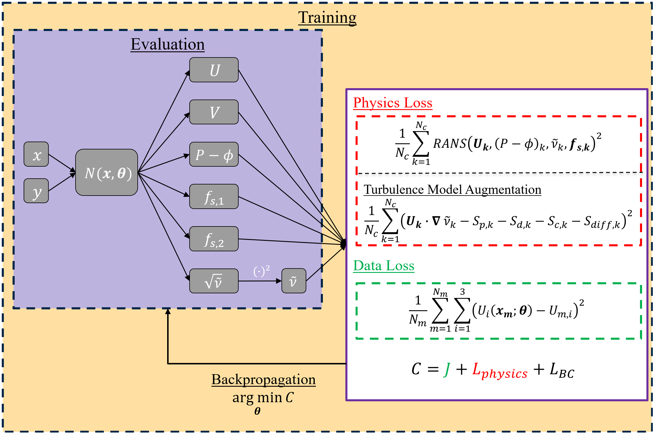
Figure 1: Structure of the Physics-Informed Neural Network. A continuous mapping between spatial coordinates and flow variables is approximated by a deep neural network, denoted by $N$, defined by a set of weights and biases, $\mathbf{\theta}$. High-fidelity coarse data measurements and the (turbulence model augmented) RANS equations constrain the training of the network.

For a PINN, the solution $(\hat{U}_{i},\hat{P}-\hat{\phi},\hat{f}_{s,i},\hat{\tilde{\nu}})(\mathbf{x;\theta})$, is defined by weights and biases, $\mathbf{\theta}$, which define a neural network. Figure 1 shows this PINN schematic. For any neural network, the optimal set of weights and biases, $\mathbf{\hat{\theta}}$, is sought by minimising some loss function $C$,

$$\hat{\theta}=\operatorname*{arg\,min}_{\mathbf{\theta}}C(U_{i},P-\phi,f_{s,i},\tilde{\nu})(\mathbf{x;\theta}).$$ (7)

In the case of PINNs, the loss function, $C$, is used to enforce the governing equations and the boundary conditions. Whilst these two terms are sufficient to define an optimisation for the forward problem, when using data assimilation (the inverse problem) the cost function must also include the measurement error term, $J$. To distinguish the use of PINNs for the inverse problem (as in this paper) compared to the forward problem, it will be referred to as PINN-DA hereon-in to emphasise the use of data. For the mean flow problem described in Section II.1, the loss function can be defined as

$$\begin{split}C=\frac{\lambda^{D}}{N_{m}}J&+\frac{\lambda^{P}}{N_{c}}\sum_{k=1}^{N_{c}}RANS\left((U_{i},P-\phi,f_{s,i},\tilde{\nu})(\mathbf{x_{k};\theta})\right)^{2}+\frac{\lambda^{P}}{N_{c}}\sum_{k=1}^{N_{c}}\left(U_{j}\frac{\partial\tilde{\nu}}{\partial x_{j}}-S_{p}-S_{diff}-S_{c}-S_{d}\right)(\mathbf{x_{k};\theta})^{2}\\ &+\frac{\lambda^{B}}{N_{b}}\sum_{b=1}^{N_{b}}BC\left((U_{i},P-\phi,f_{s,i},\tilde{\nu})(\mathbf{x_{b};\theta})\right)^{2}+\frac{\lambda^{R}}{2}\frac{1}{N_{c}}\sum_{k=1}^{N_{c}}\sum_{i=1}^{3}f_{s,i}(\mathbf{x_{k};\theta})^{2},\end{split}$$ (8)

where the governing laws are evaluated at $N_{c}$ collocation points, and boundary conditions are imposed at $N_{b}$ points along the boundary. $RANS$ is the residual of the mean flow equations ((4c) or (6d)) and $BC$ is the error to the imposed boundary conditions. To evaluate the governing laws, the gradients in the RANS equations are calculated accurately to machine-precision using automatic differentiation (leveraging the chain rule to trace the derivatives of all the constituent operations in the mapping $N(\mathbf{x,\theta})$ from Figure 1). The data term, physics term and boundary condition terms are weighted by factors $\lambda^{D},\lambda^{P}$ and $\lambda^{B}$ respectively.

The decomposition of the forcing into a modelled and corrective component (5) is not unique, as discussed in Foures et al. [26]. As a result, additional regularisation is applied to ensure uniqueness of the distribution between modelled and corrective forcing during optimisation. A regularisation term (also evaluated at collocation points) is used to control the magnitude of the corrective forcing field and subsequently the decomposition between modelled and corrective forcing, weighted by $\lambda^{R}$. For the PINN-DA, an $L_{2}$ regularisation is used. In the case without turbulence-model augmentation (effectively $\tilde{\nu}(\mathbf{x})=0$), $\lambda^{R}=0$ and the SA equation can be removed from the loss function. The total loss $C$ function (7) is minimised using backpropagation by iteratively adjusting the weights and biases based on the gradient of loss with respect to the network parameters, ${\partial C}/{\partial\mathbf{\theta}}$.

II.2.2 Variational assimilation

In the variational approach, the corrective forcing $f_{s,i}$ is adjusted such that the measurement error, $J$, is minimised, constrained by the RANS equations (6d). The solution to this minimisation problem is given by the stationary points of the Lagrangian

$$\begin{split}\mathcal{L}\left(\left[U_{i},P-\phi,\tilde{\nu},f_{s,i}\right],\left[U_{i}^{*},P^{*},\tilde{\nu}^{*}\right]\right)=J&-\langle P^{*},\frac{\partial U_{i}}{\partial x_{i}}\rangle-\langle U_{i}^{*},U_{j}\frac{\partial U_{i}}{\partial x_{j}}+\frac{1}{\rho}\frac{\partial\left(P-\phi\right)}{\partial x_{i}}-\frac{\partial(2\left(\nu+\nu_{t}\right)S_{ij})}{\partial x_{j}}-f_{s,i}\rangle\\ &-\langle\tilde{\nu}^{*},U_{j}\frac{\partial\tilde{\nu}}{\partial x_{j}}-S_{p}-S_{diff}-S_{c}-S_{d}\rangle.\end{split}$$ (9)

The inner product is defined as

$$\langle\mathbf{a},\mathbf{b}\rangle=\int_{\Omega}\mathbf{a}\cdot\mathbf{b}d\Omega,$$ (10)

where $\mathbf{a,b}$ are two spatial fields and $\Omega$ is the volume over which the field is defined. $U_{i}^{*},P^{*},\tilde{\nu}^{*}$ are the Lagrange multipliers (or adjoint variables) enforcing the constraints. By setting the variation of the Lagrangian with respect to the direct flow variables $U_{i},P-\phi,\tilde{\nu}$, one can derive the adjoint equations

$$\frac{\partial U_{i}^{*}}{\partial x_{i}}=0,$$ (11a)

$$U_{j}^{*}\frac{\partial U_{j}}{\partial x_{i}}-U_{j}\frac{\partial U_{i}^{*}}{\partial x_{j}}-\frac{\partial P^{*}}{\partial x_{i}}-\frac{\partial(2\left(\nu+\nu_{t}\right)S_{ij}^{*})}{\partial x_{j}}+\tilde{\nu}^{*}\frac{\partial\tilde{\nu}}{\partial x_{i}}+\frac{\partial}{\partial x_{j}}\left(\tilde{\nu}^{*}\partial_{\nabla U_{i}}\left(S_{p}+S_{d}\right)\right)=\frac{\partial J}{\partial U_{i}},$$ (11b)

$$-U_{j}\frac{\partial\tilde{\nu}^{*}}{\partial x_{j}}+2\frac{\partial\nu_{t}}{\partial\tilde{\nu}}\frac{\partial U_{i}^{*}}{\partial x_{j}}S_{ij}-\tilde{\nu}^{*}\frac{\partial(S_{p}+S_{d})}{\partial\tilde{\nu}}+\frac{\partial}{\partial x_{j}}\left(\tilde{\nu}^{*}\partial_{\nabla\tilde{\nu}}\left(S_{c}+S_{diff}\right)\right)=0.$$ (11c)

Furthermore, by calculating the gradient of Lagrangian, $\mathcal{L}$, with respect to changes in forcing, $\frac{\partial\mathcal{L}}{\partial f_{s,i}}$, one finds $\frac{\partial\mathcal{L}}{\partial f_{s,i}}=\frac{dJ}{df_{s,i}}=U_{i}^{*}$. Specifically, this means the gradient $\frac{dJ}{df_{s,i}}$ used to set the minimisation direction for optimisation is the solution to the adjoint equations (11c).

As with the PINN-DA-SA, regularisation is required to ensure uniqueness of the corrective forcing. Furthermore, the measurements are sparse, inducing a pointwise forcing of the adjoint momentum equations (11b) according to $\frac{\partial J}{\partial U_{i}}=2\sum_{m=1}^{N_{m}}\delta(\mathbf{x}-\mathbf{x_{m}})(U_{i}(\mathbf{x_{m}})-U_{m,i})$, which may lead to discontinues in the adjoint field and in the gradient $\frac{dJ}{df_{s,i}}$, and thus ultimately in the reconstructed forcing and corresponding mean-flow solution. This can be circumvented through $H_{1}$-like regularisation of the gradient, which consists in getting a smoothed gradient $\frac{dJ^{R}}{d\mathbf{f_{s}}}$ from the original gradient $\frac{dJ}{d\mathbf{f_{s}}}$ through the inversion of the following system

$$\begin{pmatrix}\frac{1}{1+\beta}(I-\beta\Delta)\circ&\nabla\circ\\ -\nabla\cdot\circ&0\end{pmatrix}\begin{pmatrix}\frac{dJ^{R}}{d\mathbf{f_{s}}}\\ \pi\end{pmatrix}=\begin{pmatrix}\frac{dJ}{d\mathbf{f_{s}}}\\ 0\end{pmatrix},$$ (12)

where $\beta=l_{r}^{2}$ and $l_{r}$ may be interpreted as a filter length. In the following, $l_{r}$ is chosen as the spacing between measurement locations. Eq. (12) also involves a pseudo-pressure field $\pi$ which is introduced to preserve the divergence-free character of the gradient through the regularisation procedure. A complete derivation and details of the variational approach can be found in  [26],  [28] and  [35].

It has to be noted that for high Reynolds numbers turbulent cases, the variational-based data assimilation requires the use of the SA turbulence model augmentation in order to numerically solve the discretised equations, unlike the PINNs which work (albeit with different accuracy) with and without the SA model. Previously, the laminar studies at transitional Reynolds numbers in  [26] have not required this augmentation. To distinguish this approach it shall be referred to as variational-DA-SA.

II.2.3 Comparison: PINNs vs variational assimilation

Equations (8) and (9) highlight the similarities as well as key differences between the variational-DA-SA and PINN-DA approaches. Firstly, whilst the variational-DA-SA directly adjusts the corrective forcing, through the gradient ${dJ}/{df_{s,i}}$, the PINN-DA indirectly adjusts this forcing through adjustment of the network parameters, $\mathbf{\theta}$. Secondly, by the nature of PINNs, a continuous mapping of the flow solution is obtained, which can be queried at any spatial location. Additionally, the governing equations are evaluated and enforced at discrete locations within the domain (collocation points) and the spatial gradients in this mesh-free approach are determined through automatic differentiation. In the variational-DA-SA approach, solution of the direct and adjoint equations introduces mesh dependency, where the conservation laws are enforced across the entire domain, whilst spatial gradients are calculated through discretisation (here Finite Element Method). As a result, discretisation errors are introduced, which are not present in PINNs. PINNs softly constrain the conservation laws in their continuous form whilst these are hard constraints in their discrete form for the variational-DA-SA. Lastly, the forcing regularisation method applied to the two approaches are different. The PINN-DA uses an $L_{2}$-based regularisation which was found to be sufficient to produce a smooth forcing solution. However, for the variational-DA-SA, an $L_{2}$ approach with pointwise data enforcement leads to unsmooth, pointwise forcing, thus the use of a $H_{1}$-based method, as discussed in Section II.2.2. Appendix B contains a detailed breakdown on the effect of regularisation on PINNs and the effect of different regularisers for the variational-DA-SA approach.

III Numerical Simulations and Model Setup

The PINN and variational approaches described above are applied to a canonical turbulent test case, the flow over a periodic hill. This section will describe the details of the flow case and the numerical setup of the two methods employed.

III.1 The periodic hill set-up

(a)		(b)		(c)

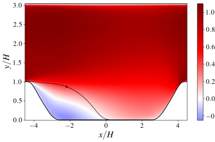
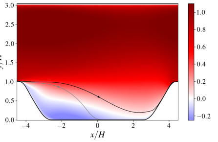
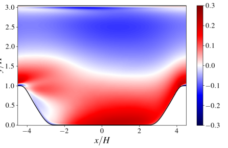
Figure 2: High-fidelity (DNS) solution of the flow over a periodic hill compared with the RANS solution using an SA model. The dividing streamline between the recirculation region and rest of the flow is shown. (a) Streamwise mean velocity - DNS; (b) streamwise mean velocity - RANS; (c) absolute error of streamwise velocity relative to DNS solution ($U_{err}=U_{DNS}-U_{RANS}$). For comparison, the DNS dividing streamline is shown in grey.

The high-fidelity data for the periodic hill is obtained from the DNS database found in using the Impact3D solver [37] and the simulation setup is detailed in Xiao et al. [38]. The DNS mean flow (time-averaged) solution, for streamwise velocity $U$ is shown in Figure 2(a). The streamline (solution to the streamfunction) dividing the recirculation region from the rest of the flow is also shown. The periodic hill is simulated at $Re=U_{b}H/{\nu}=5600$, where $H$ is the hill height, $U_{b}$ is the bulk velocity over the hill apex and $\nu$ the kinematic viscosity. Out of the several geometry configurations in the database, this work uses the canonical configuration with the domain length given by $L_{x}/{H}=3.858\alpha+5.142$ for which the hill stretch factor is $\alpha=1.0$. At this Reynolds number, separation, recirculation and reattachment are present. The no-slip condition is enforced along the upper and lower walls, whilst periodicity is enforced in the streamwise direction. In order to maintain the required massflow and thus Reynolds number, body forcing is applied in the periodic streamwise direction. This is determined at each iteration, such that the Reynolds number matches the preset Reynolds number.

To analyse the effect of data resolution on mean flow reconstruction accuracy, the high-fidelity DNS data is spatially sampled on a square grid at nine data resolutions - $0.05\leq\Delta L\leq 1.0$, where $\Delta L=\Delta x/H=\Delta y/H$. All results and figures hereon-in will compare the results from the $\Delta L=0.5$ resolution, unless otherwise stated. The measurement locations are shown in Figure 3.

The low-fidelity RANS solution with the SA turbulence model is shown in Figure 2(b,c). Whilst the DNS reattachment occurs at $x/H=0$, the RANS solver massively overpredicts the size of the recirculation region, as shown. The error field likewise shows high error across the entire domain.

III.2 PINN set-up

The PINNs are implemented using the DeepXDE Python library by Lu et al. [39], as in  [31]. This toolbox simplifies the process of building PINNs (with the Raissi et al. [21] paradigm). The code (and data) to run the PINN cases from this paper is available at https://github.com/RigasLab/PINN_SA.

All PINNs use the same architecture. The neural network was constructed as a multilayer perceptron with 7 fully connected hidden layers, each with 50 nodes. This is consistent with PINN architectures from  [31] and  [22]. The input layer consists of two nodes, representing spatial coordinates, $x/H$ and $y/H$. The output layer consists of varying number of nodes depending on the test case. The PINN initially contains five output nodes with two mean velocity components, the combined mean pressure and potential forcing field, $P-\phi$, and two solenoidal forcing nodes. When the SA turbulence model augmentation was used, an additional output node is required for $\tilde{\nu}$. Each node used a $\tanh$ activation function for its smoothness and its second order differentiability. This architecture was deemed to perform well across a range of data resolutions - further increase in nodes and layers did not equate to better performance. For PINNs, the weights and biases defining the network are randomly initialised using the Glorot uniform algorithm. This contrasts the variational-DA-SA approach, in which an “initial guess” (the RANS-SA solution) was used, around which the system is initially linearised.

For PINN optimisation, collocation points must be specified, in order to define where the governing laws are evaluated. In this work, the PINNs use 10000 collocations points which are distributed using a Hammersely distribution, such that there are sufficient points across all regions of the domain. This number of collocation points for the PINNs was selected after the reconstruction performance showed little sensitivity to further increases of the number of points. An additional 1000 points were distributed to the walls and periodic boundaries to enforce the boundary conditions. The collocation points (and domain) are shown in Figure 3. As in  [31], a two step optimisation was used for the PINNs. Initially an ADAM optimisation is applied, followed by an L-BFGS-B phase. Details on PINN convergence is discussed further in Section IV.1.

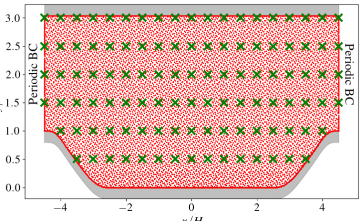
Figure 3: Turbulent periodic hill domain used for data assimilation, with $\Delta L=0.5$ data resolution (green crosses) used to compare the variational and PINN approaches. The collocation points, where the PINN evaluates residual error are in red.

III.3 Modification to PINNs for Spalart-Allmaras augmentation

Using PINNs in combination with the SA turbulence model introduces additional complexity, which require modifications to the neural network architecture and the problem formulation to achieve convergence.

Firstly, the SA transport equation contains $\frac{1}{d^{2}}$ terms in the production and destruction terms, where $d$ is the true wall distance, resulting in singularities at the wall, where $d=0$. This is not a problem for the finite element method (RANS and variational) where the residual is evaluated at a cell centre, which is not on the wall. For the PINN paradigm used, however, the governing equations are evaluated exactly at the wall boundaries and so this leads to singularities and subsequently failure to convergence. Consequently, the equation was reformulated by multiplying the SA equation with $d^{2}$ to eliminate the singularity. This new formulation can be found in Appendix A.2. Problems arising from singularities when used with PINNs have also been mentioned in [33].

The second change is to eliminate the effect of clipping negative values of $\tilde{\nu}$. The negative SA equation formulation used in the variational approach has distinct equations for positive and negative $\tilde{\nu}$ (detailed in Appendix A.1) to ensure the transport equation is continuous across both positive and negative $\tilde{\nu}$. The final eddy viscosity, $\nu_{t}$, is then clipped at negative values of $\tilde{\nu}$ and set to zero, resulting in only positive values of $\nu_{t}$. Convergence of the PINNs is improved when the complexity caused by the discontinuity from clipping $\nu_{t}$ is removed. Thus, to enforce positive $\tilde{\nu}$, the output of the neural network is defined as $\sqrt{\tilde{\nu}}$. A transformation is then applied to the output, squaring the value, to produce a positive $\tilde{\nu}$. This is shown in Figure 1.

III.4 Variational assimilation set-up

Both the solution of the RANS-SA system (shown in Figure 2(b)) and the variational assimilation system are obtained using a finite-element method (FEM) spatial discretisation implemented in FreeFEM++ [40]. Piecewise-linear functions that are enriched by bubble functions are used for velocity and pseudo-turbulent viscosity variables, while piecewise-linear functions are used for pressure. The FEM is known to be unstable at high Reynolds numbers. Accordingly, both streamline-upwind Petrov-Galerkin (SUPG) [41, 28] and grad-div [42] formulations are here employed to stabilise the method. A low-memory Broyden–Fletcher–Goldfarb–Shanno (L-BFGS) [43] algorithm is used to exploit the gradient $\frac{dJ^{R}}{d\mathbf{f_{s}}}$ from (12) in order to perform the minimisation of the cost function $J$ in (1). Further details on the implementation of the variational-DA-SA can be found in [28, 35].

IV Results

(a)		(b)		(c)

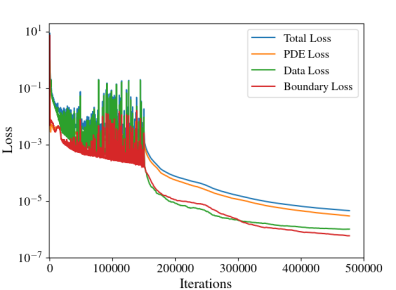
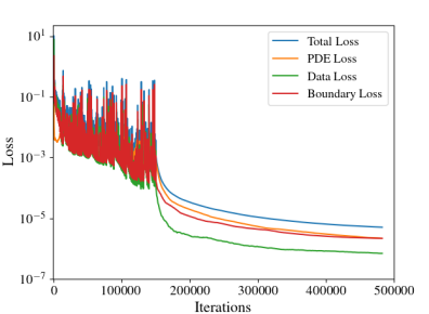
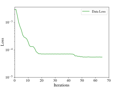
Figure 4: Residual loss during optimisation for (a) PINN-DA-Baseline, (b) PINN-DA-SA and (c) Variational-DA-SA. For PINN optimisation (training), there are two distinct phases: the ADAM (stochastic gradient descent based) optimisation for 150000 iterations followed by the L-BFGS-B phase.

Table 1: Loss function weights used in PINN optimisation. For PINN-DA-Baseline, the $\tilde{\nu}$ weight can be ignored.

Weight	$\lambda^{P}$	$\lambda^{D}$	$\lambda^{B}(U_{i})$ - Wall	$\lambda^{B}(\tilde{\nu},f_{s,i})$ - Wall	$\lambda^{B}$ - Periodic
Value	1	10	2.5	10	1

We compare the mean flow reconstruction from sparse mean velocity measurements for the turbulent periodic hill case using three approaches: PINN-DA-Baseline (without turbulence model), PINN-DA-SA (with SA) and variational-DA-SA (with SA). Firstly, an evaluation of the PINN-DA-Baseline approach is presented. Secondly, we will show that significant reduction in reconstruction error is achieved by augmenting the PINN-DA-Baseline approach with the SA turbulence model (PINN-DA-SA). Thirdly, we compare it directly to the variational-DA-SA showing the increased accuracy of the PINN-DA-SA relative to the variational-DA-SA.

To evaluate the mean flow reconstruction accuracy, a volume weighted $L_{2}$ error will be used and is calculated as

$$\varepsilon_{2}=\sqrt{\frac{1}{\Omega}\sum_{n=1}^{N}\delta\Omega_{n}\sum_{i=1}^{2}\left(U_{n,i}-\hat{U}_{i}(\mathbf{x_{n}})\right)^{2}},$$ (13)

where $\Omega$ is the volume of the domain, $\delta\Omega_{n}$ is the cell volume of each point used to determine the error (as defined by the DNS grid) and $N$ is the number of points across the domain. $U_{n,i}$ is the high fidelity, DNS mean velocity at $\mathbf{x_{n}}$ and $\hat{U}_{i}(\mathbf{x_{n}})$ is the corresponding reconstructed mean velocity.

IV.1 Optimisation

Figure 4 shows the optimisation convergence of the PINN-DAs (a,b) and the variational-DA-SA approach (c). The PINN-DA loss convergence curve is decomposed into three loss components - PDE residual, data error and boundary condition error. For PINN-DA-SA the additional loss from the SA transport equation contributes also to the PDE loss. Each individual loss component appearing in Eq. (8) was given initial weight values $\lambda$ based on the relative magnitudes of the flow variables. This was followed by several weight tuning steps to find the best combination, as compiled in Table 1. During the first phase of the training, ADAM optimisation is performed for 150000 iterations. The second phase applies L-BFGS-B optimisation for 300000 iterations or until the model has sufficiently converged to the floating point tolerance. Figures 4(a,b) shows that during optimisation (for both PINN-DA methodologies), the ADAM phase reduces loss from the high value caused by the initial randomised state to approximately $10^{-3}$. The L-BFGS-B phase is then used to fine tune the optimisation, reducing total loss to below $10^{-5}$.

The convergence of the variational-DA-SA, seen in Figure 4(c) shows the data loss, corresponding to $J/N_{m}$, where $J$ is defined in (1). This data loss is equivalent to the corresponding curves in Figures 4(a,b). Whilst convergent, the data loss is an order of magnitude higher for the variational-DA-SA compared with the PINN-DAs.

IV.2 PINN-DA-Baseline

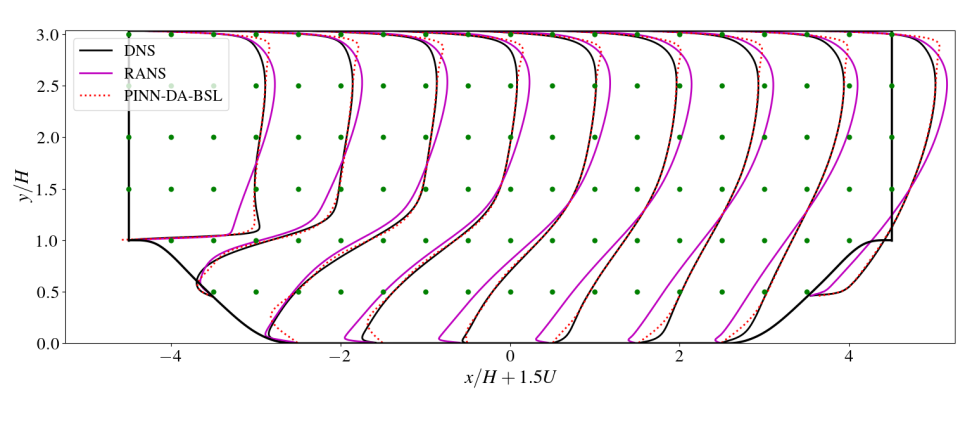
Figure 5: Streamwise velocity profiles for DNS, RANS-SA and PINN-DA-Baseline.

Here, the PINN-DA-Baseline approach is applied to reconstruct the mean flow velocity field when coarse mean flow velocity data is available with spacing $\Delta L=0.5$. This is compared against the DNS and RANS-SA velocity profiles in Figure 5. The data assimilation of the high fidelity measurements has improved the prediction of the velocity field compared to RANS-SA. The total mean velocity $L_{2}$ error is $3.60\times 10^{-2}$ instead of the $8.99\times 10^{-2}$ error from RANS-SA. High accuracy of reconstruction is observed in the bulk flow domain. However, high mean velocity reconstruction error is observed in areas with high velocity gradients, such as near the walls and at separation. This is most apparent at the upper wall boundary layer. This near wall error accounts for over 40% of the total $L_{2}$ error as the PINN-DA-Baseline fails to accurately capture high-gradient flow features. These trends are highlighted in the streamwise velocity contours in Figure 6(a,d). At data points, the PINN-DA-Baseline reproduces the measurements accurately. Furthermore, in spite of the higher near-wall reconstruction errors, Figure 6(a) shows improved reconstruction of the recirculation bubble, even with limited data in this area. This is most noticeable when comparing the PINN-DA-Baseline bubble from Figure 6(a) with the RANS bubble in Figure 2(b). The provision of sparse high-fidelity datapoints in the PINN-DA-Baseline approach has enabled better prediction of the shape of the recirculation region. However, the error field makes the limitation of the PINN-DA-Baseline approach more apparent, with the near wall errors particularly noticeable.

The results of PINN-DA-Baseline show that the methodology used in  [31] for laminar flow can also be used for turbulent flows. In  [31], the base formulation of the RANS equations (as in (2b)) was also tested. It was shown that by providing data for both first order (mean velocity) and second order (Reynolds stresses) statistics, the PINN-DA-Baseline was able to reconstruct the pressure field for the laminar case. This approach has been demonstrated in Appendix C. With similar mean velocity reconstruction accuracy, this second approach was also able to infer the pressure field for this turbulent case.

IV.3 PINN-DA-SA

This section contains results from the augmentation of the SA model to PINNs. First, a comparison between the PINN-DA-Baseline and PINN-DA-SA results will be presented, followed by a discussion on the improved reconstruction when the SA model is used. Finally, the results of the variational data assimilation using SA (variational-DA-SA) are also presented, followed by a parametric analysis of the data resolution.

IV.3.1 PINN-DA-SA vs PINN-DA-Baseline

		PINN-DA-Baseline		PINN-DA-SA		Variational-DA-SA
	(a)		(b)		(c)
$\hat{U}$
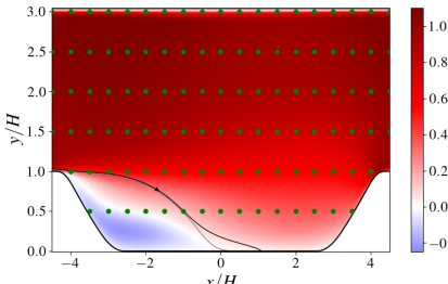
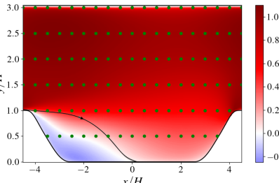
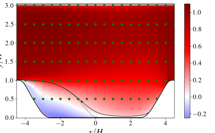
	(d)		(e)		(f)
$U_{err}$

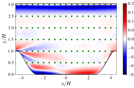
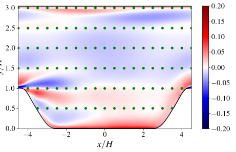
Figure 6: Reconstructed $U$ velocity component for the PINN-DA-Baseline (left), PINN-DA-SA (middle), variational-DA-SA (right) approaches. (a,b,c) - $U$ reconstruction. (d,e,f) - Absolute $U$ error. PINN-DA-SA performs best, significantly reducing the separation error seen in other approaches, whilst also reducing the near wall error seen in PINN-DA-Baseline. The dividing streamline (separating the recirculation region) is shown in (a,b,c) and compared with the DNS equivalent (in grey). Whilst the PINN-DA-SA recirculation region is indistinguishable, there is a small but noticeable difference for the PINN-DA-Baseline and variational-DA-SA solutions.

Figure 6(a,d) shows the PINN-DA-Baseline and Figure 6(b,e) the PINN-DA-SA reconstruction results. Streamwise velocity and error contours relative to the DNS solution are shown, with similar trends holding for the vertical velocity component (not shown here). Whilst the error field topologies are qualitatively similar, the magnitude error is significantly reduced. For PINN-DA-SA, the recirculation bubble is almost indistinguishable from the DNS one. As a consequence of introducing the Spalart-Allmaras model, reconstruction error has reduced by 63% ($\varepsilon_{2}=1.35\times 10^{-2}$). For the bulk flow region above the hills and away of the walls (between $y/H=1.5$ and $y/H=2.5$) and at datapoints, the PINN-DA-SA and PINN-DA-Baseline show similarly low reconstruction errors. This is expected in this region given the lack of mean shear and production of turbulent kinetic energy.

Comparing the PINN-DA-Baseline error against the PINN-DA-SA highlights the effect of augmenting the PINN with the SA turbulence model. The high mean flow error along the upper wall has largely reduced indicating that use of the SA model has enabled a better reconstruction of the near-wall region. There are also similarly significant improvements along the lower wall both at separation but also after reattachment. The improvements of PINN-DA-SA compared to PINN-DA-Baseline corroborate well with the original design purpose and performance of the SA turbulence model, which shows improved performance for turbulent boundary layers in adverse pressure gradients.

IV.3.2 Why PINN-DA-SA?

In order to understand the difference in performance between PINN-DA-Baseline and PINN-DA-SA, we examine the individual terms of the cost function, $C$, for each approach. This consists of the measurement error term (data loss) and the enforcement of the governing equations (PDE loss).

Firstly, we examine the data loss component. Inspection of Figure 6(d) reveals that the PINN-DA-Baseline reconstructs the mean velocity measurements accurately. This is comparable to the performance of the PINN-DA-SA, with the convergence plots in Figure 4(a,b) showing similar converged data loss values. Away from the data points, the reconstruction error increases substantially for the PINN-DA-Baseline. This is most apparent along the upper wall where a high error region exists above the data at $y/H=2.5$. Given that the reconstruction error is low at the data points for PINN-DA-Baseline (and also similar to PINN-DA-SA), further decrease of the error to measurements, $J$, does not reduce the mean velocity error away from datapoints, where most of the reconstruction error lies.

Secondly, one can consider the other component of the cost function, the residual PDE error. Figure 7(a) shows the PINN-DA-Baseline momentum residual error (for x- and y-momentum equations). The PDE residual error contour shows that there is a limited correlation between mean velocity reconstruction error and residual error from the conservation laws - most apparent along the upper and lower walls. A similar analysis for the PINN-DA-SA corroborates this trend (Figure 7(b)). The total residual PDE loss from both PINN-DA-Baseline and PINN-DA-SA (seen in Figure 4) are of similar magnitudes (approx. $10^{-5}$) and the residual PDE fields are comparable, despite the significant differences in reconstruction accuracy between the two PINN-DA approaches. This indicates that further reduction in the residual PDE error does not lead to increase in reduction in reconstruction error and thus cannot be attributed as the cause of the difference between PINN-DA-Baseline and PINN-DA-SA.

The difference between PINN-DA-Baseline and PINN-DA-SA can be consequently attributed to the effect of the turbulence model augmentation. Due to the unclosed (underdetermined) nature of the RANS equations, there are infinite solutions to the forcing (divergence of Reynolds stress tensor) in the mean flow equations. Providing high-fidelity data measurements “anchors” the PINN-DA solution at these discrete data points. However, away from them, there are still many candidate solutions to the mean flow, as the governing equations are still under-determined. These solutions all satisfy the governing equations and thus all have low residual PDE error. There are consequently no terms within the optimised cost function (Eq. (8)) that can be minimised further, to reduce the mean velocity reconstruction error across the domain for PINN-DA-Baseline. The current optimisation for PINN-DA-Baseline is converged towards a solution that obeys the under-determined RANS equations. This is also briefly mentioned in Foures et al. [26]. The SA model adds physics constraints that limit further the infinite number of admissible solutions far from the measurement points and as a direct consequence lead to improved reconstruction.

	PINN-DA-Baseline		PINN-DA-SA
(a)		(b)

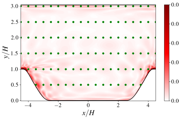
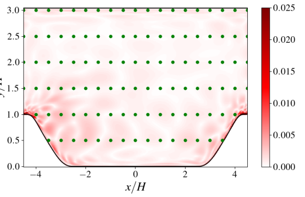
Figure 7: PDE residual error (x-momentum and y-momentum). (a) PINN-DA-Baseline and (b) PINN-DA-SA. The residual error between approaches are comparable despite the considerable improvements in mean velocity reconstruction error demonstrated by the PINN-DA-SA.

IV.3.3 Variational-DA-SA results and comparison with PINNs

The PINN-DA-SA can be directly compared to the variational-DA-SA, which also uses SA augmentation, since both methods use the same data and physics constraints. Figures 6(c,f) show the reconstructed mean streamwise velocity and the respective absolute error for the variational-DA-SA. As with all the data assimilation results presented, the key flow features (separation, recirculation bubble and reattachment) are well reconstructed. As with both PINN-DA methodologies, the variational-DA-SA reconstructs the shape of the recirculation bubble more accurately than the RANS-SA, despite the limited measurements in this region. The reconstruction error matches the features seen in the PINN-DA results as well as in [26], with high error between data points, near walls and at the initial separation.

The key feature seen in the comparison between variational-DA-SA and PINN-DA-SA is that the latter has demonstrably lower error across all regions of flow. The highest reduction in error in the PINN-DA-SA is observed in the region between hills ($y/H\leq 1.0$), specifically the recirculation and separation. Whilst all approaches have topologically similar error fields (such as the initial the separation), the PINN-DA-SA demonstrates a vastly reduced error. At data points, the reconstruction error is much lower for PINN-DA approaches than the variational-DA-SA. Figure 4 shows that the PINN-DA’s have measurement error of the order of $10^{-7}$ whilst the variational-DA-SA is $10^{-5}$. The relative performance of the variational-DA-SA and PINN-DA-SA compared with both RANS-SA and the DNS flow can be summarised in the velocity profiles in Figure 8. Whilst both data assimilation methods represent a significant improvement over a RANS-SA simulation, the PINN-DA-SA is almost identical to the DNS results, whilst small discrepancies are still more apparent for the variational-DA-SA.

Comparing both PINN-DA-SA and variational-DA-SA to PINN-DA-Baseline show that application of SA has been successfully used to reduce error for near-wall gradients, as a result of the additional physical description provided by the turbulence model. The specific choice of turbulence model (SA) is also a contributing factor, given the aforementioned good performance in boundary layers with adverse pressure gradients.

The lower reconstruction error of the PINN-DA-SA approach compared to the variational-DA-SA approach has been confirmed also for the laminar case, in the absence of the SA model. The test case for this was the unsteady cylinder flow at low Reynolds numbers. Appendix D includes details on the laminar flow case, followed by a comparison of results.

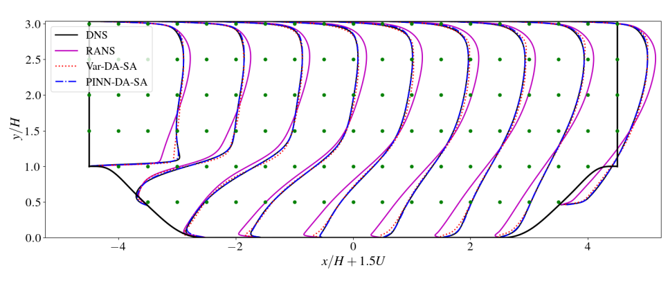
Figure 8: Mean flow reconstruction of streamwise velocity profiles for DNS, RANS-SA, PINN-DA-SA and variational-DA-SA.

		$f_{1}$		$f_{2}$
	(a)		(b)
PINN-DA-Baseline
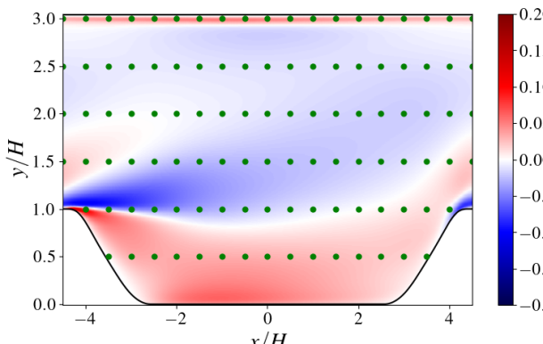
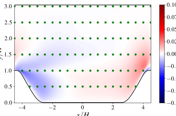
	(c)		(d)
PINN-DA-SA
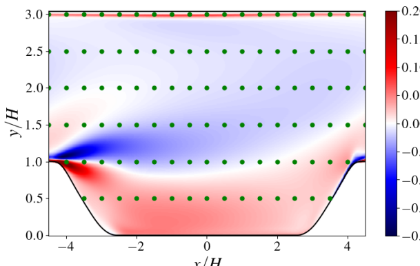
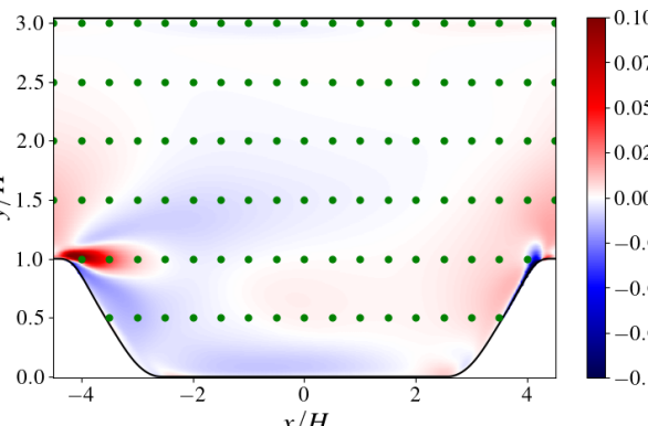
	(e)		(f)
Variational-DA-SA

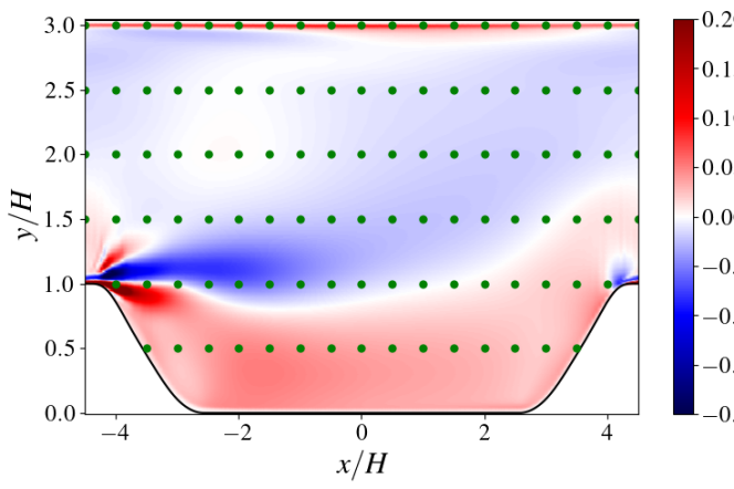
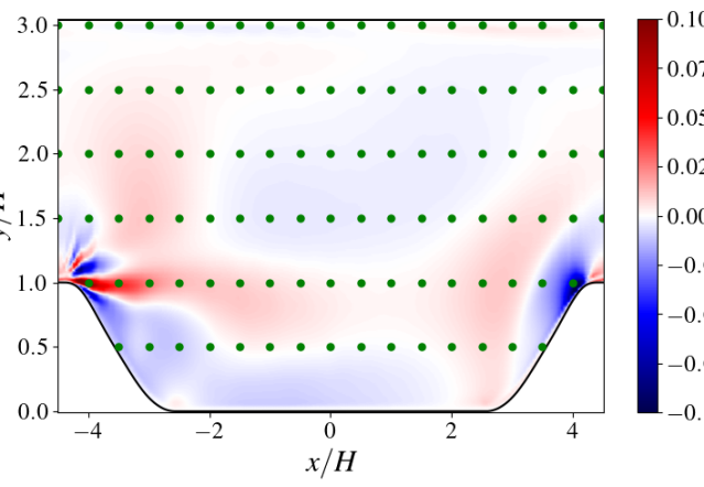
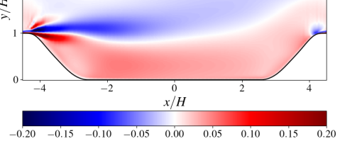
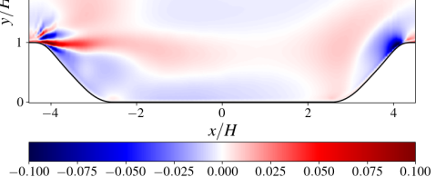
Figure 9: A breakdown of the Reynolds forcing (excluding the potential field) $f_{1}$ (left) and $f_{2}$ (right) from the different methodologies: $f_{i}=\frac{\partial(2\nu_{t}S_{ij})}{\partial x_{j}}+f_{s,i}$. For PINN-DA-Baseline, $\nu_{t}=0$. These are (a,b) - PINN-DA-Baseline, (c,d) - PINN-DA-SA, (e,f) - Variational-DA-SA.

(a)	DNS	(b)	Variational-DA-SA
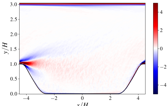
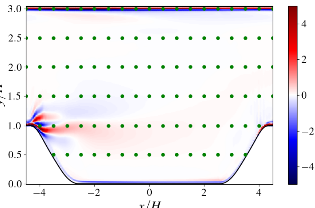
(c)	PINN-DA-Baseline	(d)	PINN-DA-SA

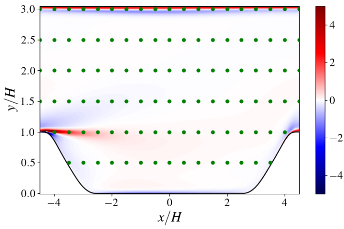
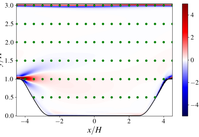
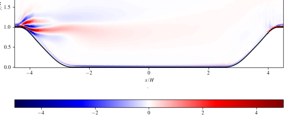
Figure 10: $\nabla\times\mathbf{f}$. Comparison of curl(f) between the ground truth (DNS) and the different data assimilation techniques presented in this paper. (a) DNS, (b) Variational-DA-SA, (c) PINN-DA-Baseline, (d) PINN-DA-SA.

IV.3.4 Forcing fields

The inferred forcing given by Eq. (5) consists of solenoidal and modelled eddy viscosity (SA contribution) components. For PINN-DA-Baseline, the modelled eddy viscosity component is zero. A further analysis of the forcing terms allows isolation of the effect of SA in the accurate reconstruction of the mean flow field.

The PINN-DA-Baseline and PINN-DA-SA forcing fields shown in Figure 9 are qualitatively similar in the uniform flow region between $y/H=1.5$ and $y/H=2.5$, where turbulent production is low. However, the regions of the flow where PINN-DA-Baseline shows high levels of error (as seen in Figure 6(d)) result in larger forcing changes in the PINN-DA-SA solution. Introduction of a modelled component (via SA) has led to a significant changes to the corrective forcing, most notably at the separation but also near the walls. These changes underpin the differences in reconstruction error between PINN-DA-Baseline and PINN-DA-SA. Constraining the solution with additional physical definition (via SA) has provided additional modelled forcing in regions where data-assimilation methods with the under-determined RANS had the highest errors. Whilst the PINN-DA-Baseline had converged to a poor solution, the PINN-DA-SA has reduced the “amount” of under-determined forcing resulting in lower reconstruction errors. However, the addition of the corrective term, which is still unclosed, has allowed the data-assimilation approach to correct the SA model.

The PINN-DA-SA forcing is different to the variational-DA-SA forcing, in accordance to the differences in mean flow reconstruction. In general, the PINN-DA-SA forcing is closer to the variational-DA-SA forcing than the PINN-DA-Baseline forcing. However, there are several differences in forcing, appearing in regions with the largest differences in reconstruction. This is most apparent in the significantly less smooth forcing around the separation in the variational-DA-SA forcing compared to PINN-DA-SA. There is also a large difference in $f_{2}$ forcing along the rear hill, centred around a datapoint. This datapoint (in the $\Delta L=0.5$ case) has shown to be particularly sensitive.

To evaluate the accuracy of the data assimilation methods, the forcing is also compared with the true DNS forcing. As the potential forcing field is absorbed into the pressure term and thus is inseparable, we instead compare the curl of forcing, to remove the contribution of the potential forcing (since $\mathbf{\nabla\times\nabla}\phi)=0$).

$$(\mathbf{\nabla\times f})_{3}=\frac{\partial f_{s,2}}{\partial x}-\frac{\partial f_{s,1}}{\partial y}+\left(\frac{\partial^{2}}{\partial x^{2}}-\frac{\partial^{2}}{\partial y^{2}}\right)2\nu_{t}S_{12}+\frac{\partial^{2}}{\partial x\partial y}\left(2\nu_{t}(S_{22}-S_{11})\right).$$ (14)

A direct comparison can be performed then against the curl of the DNS forcing

$$(\mathbf{\nabla\times f})_{3}=\frac{\partial f_{2}}{\partial x}-\frac{\partial f_{1}}{\partial y}=\left(\frac{\partial^{2}}{\partial x^{2}}-\frac{\partial^{2}}{\partial y^{2}}\right)\overline{{u}^{\prime}{v}^{\prime}}+\frac{\partial^{2}}{\partial x\partial y}\left(\overline{{v}^{\prime}{v}^{\prime}}-\overline{{u}^{\prime}{u}^{\prime}}\right).$$ (15)

The curl of the inferred forcing for all three reconstruction methods employed here is shown in Figure 10. Best agreement with the DNS is achieved for PINN-DA-SA, which aligns with the most accurate mean flow reconstruction. The PINN-DA-Baseline differs from DNS in several key regions - the initial separation, the recirculation, the rearward hill apex and along the walls. Differences between the variational-DA-SA and PINN-DA-SA forcing (and curl) correlate with differences in the error fields. These are most apparent at the separation region and along the upper and lower walls.

IV.3.5 Data Assimilation with varying data resolution

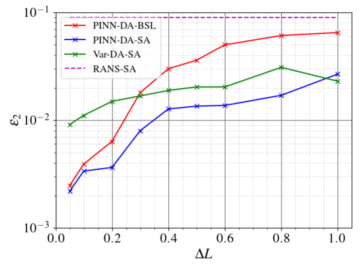
Figure 11: Volume-weighted $L_{2}$ mean velocity reconstruction error (as defined in Eq. (13)) versus data resolution for the three reconstruction methodologies (solid lines with symbols). All three approaches improve the RANS-SA predictions (dashed line).

Here, we evaluate the dependence of the reconstruction error on the data resolution of the available high-fidelity measurements. In Figure 11, we compare variational-DA-SA, PINN-DA-Baseline and PINN-DA-SA approaches, for a range of data-resolutions, ranging form $\Delta L=0.05$ to $\Delta L=1.0$. The reconstruction error increases monotonically as the (equidistant/square) spacing between data points increases. All data assimilation methods improve the RANS-SA solution, irrespective of resolution. For data spacing $\Delta L<1$, the turbulence model augmented PINN-DA-SA method achieves the lowest reconstruction error against all the other methods.

Comparing the PINN-DA-Baseline to the PINN-DA-SA results shows the significant improvement achieved through the turbulence model augmentation. The gap between the two can mostly be attributed to the error near the walls and in the separation. Additionally, the rate of error increase with respect to data resolution is steeper for PINN-DA-Baseline, suggesting reduced dependence on data with the addition of a modelled (closed) forcing component. In fact, as data resolution becomes finer, the two PINN-DA approaches converge. This is expected - as more data is provided, there are more points at which the PINN-DA-Baseline can close the solution and thus the advantage the turbulence model augmentation provides is diminished.

Comparing the PINN-DA-SA versus the variational-DA-SA solution shows that, for most of the resolution range, the PINN-DA-SA also demonstrates consistently lower error at equivalent resolutions. In fact, the PINN-DA-SA at $\Delta L=0.8$ matches the reconstruction accuracy of the variational-DA-SA at $\Delta L=0.3$. However, at the extreme end of coarse data ($\Delta L=1.0$), whilst the PINN-DA-SA is still a significant improvement over the PINN-DA-Baseline (and also RANS-SA), the variational-DA-SA approach has a lower reconstruction error. This suggests that the PINNs have a greater dependence on data for good performance. As data resolution reduces (spacing increases), the optimisation problem converges to solving the direct RANS-SA problem, for which the numerical framework within the variational-DA-SA method is more robust i.e. PINNs are less effective forward solvers. Algorithmic improvements for PINNs, including adaptive weighting algorithms, can potentially provide further improvements of the PINN approach, which is currently under investigation. On the opposite end, for fine data resolutions, the variational-DA-SA is less accurate than the PINN-DA-Baseline.

One may attribute the difference between the reconstruction accuracy of the PINN-DA-SA and variational-DA-SA to the differences in the way the RANS equations are enforced in the data assimilation procedure. Concerning the variational-DA-SA approach, it may be first noticed that the latter solves for only the weak form of the RANS equations, following the finite-element approach. In addition, as mentioned in Section III.4, stabilisation terms are added in the governing equations. Then there is the process of spatial discretisation through, among others, the choice of shape functions, which will determine the order of spatial accuracy. In contrast, PINNs enforce the RANS equations in their original, strong formulation, and in a continuous way. Moreover, the effect of applying discrete pointwise forcing at measurement locations poses a greater challenge for the variational approach than PINNs and thus the method of regularisation has a greater impact on reconstruction performance. Appendix B.2 contains analysis of regularisation choice. By avoiding both these sources of error, PINN-DA-SA achieve a lower reconstruction error than the variational-DA-SA. This is evidenced by the reconstruction error for finer data resolutions. Even as data resolution increases, the aforementioned discretisation error remains. Consequently, the reconstruction error of the variational-DA-SA reduces at a much slower rate than both PINN-DAs.

V Conclusion

Three approaches to turbulent mean flow reconstruction from sparse data measurements have been presented and compared. For all methods, inferring the closure of the underdetermined RANS equations or the corrective closure of the RANS-SA equations by assimilating high-fidelity sparse data improved the mean flow reconstruction compared to RANS-SA predictions. The use of Spalart-Allmaras turbulence model, as used in  [28] (in the variational-DA-SA approach) was proposed for use in PINNs, particularly in the context of turbulent flows. The SA turbulence model augmented PINN (PINN-DA-SA) proved to be the most accurate flow reconstruction method followed by the equivalent approach albeit with a variational formulation.

Comparing the PINN-DA-Baseline (PINN without turbulence SA model) with PINN-DA-SA showed the isolated effect of turbulence model augmentation. The PINN-DA-SA performs significantly better in regions with complex flow features, such as near walls and at separation. Injection of additional physical constraints in the form of a turbulence model provides an additional modelled component to the underdetermined Reynolds forcing, reducing the complexity of the optimisation and narrowing the solution space for the optimisation. A corrective forcing term is then tuned to correct the rest of the closure. The variational-DA-SA approach, whilst an improvement over the PINN-DA-Baseline, has higher errors compared to the PINN-DA-SA, most notably off the separation. These observations for mean flow reconstruction accuracy are also associated with equivalent error in Reynolds forcing. The difference in variational-DA-SA and PINN-DA-SA can be attributed to the effect of discretisation, which is avoided by PINNs. These observations are consistent across different data resolutions.

Given that PINNs is a growing field of research, there are potentially many avenues to improve the reconstruction capability further. The most apparent example is hyper-parameter tuning, such as loss weighting. In this study, a static weighting method was used with manual iterations to tune them. This is a laborious exercise, particularly as systems become more complex with more boundary conditions and less uniform topologies. Adaptive weighting algorithms [44, 45] or novel architectures, such as Competitive PINNs [46], would both simplify this problem and also generalise the process to selecting weights.

Appendix A Spalart-Allmaras equations

The full definition of the SA transport equations, as mentioned in Equation (6d), is described here.

A.1 Formulation of Spalart-Allmaras equations

The Spalart-Allmaras equations are solved for $\tilde{\nu}$. Then, the eddy viscosity, $\nu_{t}$, is obtained as

$$\nu_{t}=\begin{cases}0&\text{ if }\tilde{\nu}<0,\\ f_{v1}\tilde{\nu}&\text{ if }\tilde{\nu}\geq 0,\end{cases}$$ (16)

where

$$f_{v1}=\frac{\chi^{3}}{\chi^{3}+c_{v1}^{3}},\hskip 10.0pt\chi=\frac{\tilde{\nu}}{\nu}.$$ (17)

The SA transport equation takes the form

$$U_{j}\frac{\partial\tilde{\nu}}{\partial x_{j}}-S_{p}-S_{diff}-S_{c}-S_{d}=0,$$ (18)

where $S_{p},S_{diff},S_{c},S_{d}$ are production, diffusion, cross-diffusion and destruction terms respectively. These are defined as

$$\begin{array}[]{cc}S_{p}=\begin{cases}c_{b1}S\tilde{\nu}g_{n}&\text{ if }\tilde{\nu}<0,\\ c_{b1}\tilde{S}\tilde{\nu}&\text{ if }\tilde{\nu}\geq 0,\end{cases}&S_{d}=\begin{cases}c_{w1}\frac{\tilde{\nu}^{2}}{d^{2}}&\text{ if }\tilde{\nu}<0,\\ -c_{w1}f_{w}\frac{\tilde{\nu}^{2}}{d^{2}}&\text{ if }\tilde{\nu}\geq 0,\end{cases}\\ S_{diff}=\frac{1}{\sigma}\nabla\cdot(\eta\nabla\tilde{\nu})=\frac{1}{\sigma}\left(\eta\frac{\partial^{2}\tilde{\nu}}{\partial x_{j}^{2}}+\frac{\partial\eta}{\partial x_{j}}\frac{\partial\tilde{\nu}}{\partial x_{j}}\right),&\hskip 15.0ptS_{c}=\frac{c_{b2}}{\sigma}\left\|\nabla\tilde{\nu}\right\|^{2}=\frac{c_{b2}}{\sigma}\left(\frac{\partial\tilde{\nu}}{\partial x_{j}}\right)^{2}.\end{array}$$ (19)

where the auxillary functions and constants are defined as

$$\begin{array}[]{ccc}\eta=\begin{cases}\nu(1+\chi+\frac{1}{2}\chi^{2})&\text{ if }\tilde{\nu}<0,\\ \nu(1+\chi)&\text{ if }\tilde{\nu}\geq 0,\end{cases}&{S}^{\prime}=\left\|\nabla\times\mathbb{U}\right\|,&{S}=\sqrt{{S}^{\prime 2}+M^{2}}-M,\\ \overline{S}=\frac{\tilde{\nu}f_{v2}}{\kappa^{2}d^{2}},&f_{v2}=1-\frac{\chi}{1+\chi f_{v1}},&\tilde{S}=max(10^{-10},S+\overline{S}),\\ {r}^{\prime}=\frac{\tilde{\nu}}{\tilde{S}\kappa^{2}d^{2}},&r=\begin{cases}{r}^{\prime}&\text{ if }0\geq{r}^{\prime}\geq 10,\\ 0&\text{ otherwise, }\end{cases}&g=r+c_{w2}(r^{6}-r),\\ f_{w}=g\left(\frac{1+c_{w3}^{6}}{g^{6}+c_{w3}^{6}}\right)^{\frac{1}{6}},&&g_{n}=1-\frac{1000\chi^{2}}{1+\chi^{2}}.\end{array}$$ (20)

The constants in the SA transport equations are $c_{v1}=7.1$, $c_{v2}=0.7$, $c_{v1}=0.9$, $\kappa=0.41$, $\sigma=\frac{2}{3}$, $c_{b1}=0.1355$, $c_{b2}=0.622$, $c_{w1}=\frac{c_{b1}}{\kappa^{2}}+\frac{1+c_{b2}}{\sigma}$, $c_{w2}=0.3$, $c_{w3}=2$.

A.2 Wall-Distance multiplied Spalart-Allmaras Equations

To remove singularities, which causes problems for the PINN-DA-SA formulation at points evaluated at (or near) the wall (as discussed in Section III.3), the modified SA equations take the form

$$d^{2}\left(U_{j}\frac{\partial\tilde{\nu}}{\partial x_{j}}-S_{diff}-S_{c}\right)-S_{p}^{N}-S_{d}^{N}=0,$$ (21)

where $S_{p}^{N},S_{d}^{N}$ are new modified production and destruction terms respectively. These are defined as

$$\begin{array}[]{cc}S_{p}^{N}=d^{2}S_{p}=\begin{cases}c_{b1}S^{N}\tilde{\nu}g_{n}&\text{ if }\tilde{\nu}<0,\\ c_{b1}\tilde{S}^{N}\tilde{\nu}&\text{ if }\tilde{\nu}\geq 0,\end{cases}&\hskip 15.0ptS_{d}^{N}=d^{2}S_{d}=\begin{cases}c_{w1}\tilde{\nu}^{2}&\text{ if }\tilde{\nu}<0,\\ -c_{w1}f_{w}\tilde{\nu}^{2}&\text{ if }\tilde{\nu}\geq 0.\end{cases}\end{array}$$ (22)

The modified auxiliary functions are thus

$$\begin{array}[]{cc}S^{N}=d^{2}S=d^{2}\left(\sqrt{{S}^{\prime 2}+M^{2}}-M\right),&\overline{S}^{N}=d^{2}\overline{S}=\frac{\tilde{\nu}f_{v2}}{\kappa^{2}},\\ \tilde{S}^{N}=d^{2}\tilde{S}=max(10^{-10},d^{2}\left(S+\overline{S}\right))=max(10^{-10},S^{N}+\overline{S}^{N}),&{r}^{\prime}=\frac{\tilde{\nu}}{\tilde{S}^{N}\kappa^{2}}.\end{array}$$ (23)

Appendix B Effect of regularisation on data assimilation techniques

As mentioned in Section II.2, the forcing decomposition between modelled and corrective parts is not unique and thus the regularisation of corrective forcing is critical. This section will show the effect of regularisation for both PINN-DA and variational approaches and highlight its importance.

B.1 Effect of solenoidal forcing regularisation on PINNs

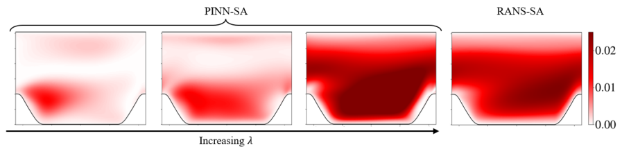
Figure 12: Effect of regularisation parameter (solenoidal forcing magnitude penalisation), $\lambda^{R}$ on PINN-SA solution for $\tilde{\nu}$. $\tilde{\nu}$ for increasing $\lambda^{R}$ compared with the RANS-SA $\tilde{\nu}$ shows that increasing regularisation causes eddy viscosity to converge towards the RANS solution. The presented values of $\lambda^{R}$ are $10^{-8}$, $10^{-4}$, $10^{0}$ left to right

For PINN-DA-SA, an $L_{2}$ penalisation of the solenoidal forcing magnitude was applied. During PINN-DA-SA hyper parameter tuning, it was found that the final solution was strongly influenced by the regularisation of solenoidal forcing. Clearly as regularisation weight, $\lambda^{R}$, increases, the magnitude of solenoidal forcing is penalised more and thus there is a greater dependence on the modelled eddy viscosity forcing component. In effect, the greater the value of $\lambda$, the closer the governing equations tend towards a pure RANS-SA problem. However, for the PINN-DA, enforcement of data loss at measurement points results in differences. This is demonstrated in Figure 12. As solenoidal forcing magnitude is penalised more and more, the solution tends towards RANS-SA. However, this is an imperfect solution as the PINN-DA-SA is attempting to fit high fidelity (mean) DNS data to the RANS-SA equations. This is most notable at the point around the rear hill apex. As a result, the residual PDE loss begins to increase at very high $\lambda^{R}$. On the other hand, without penalisation ($\lambda^{R}=0$), the PINN-DA-SA solution tends towards the PINN-DA-Baseline solution with a negligible contribution from the eddy viscosity component ($\tilde{\nu}\approx 0$).

As the data coarsens, and thus the dependence on data reduces, the requirement for a modelled component becomes more important, as the corrective Reynolds forcing can be closed at fewer points using data. Less data means the solution will move closer to a RANS-SA solution. As a result, the coarser the data, the greater the value for the optimal $\lambda^{*}$, as the modelled forcing component becomes a greater component of the forcing. This is seen in Figure 13.

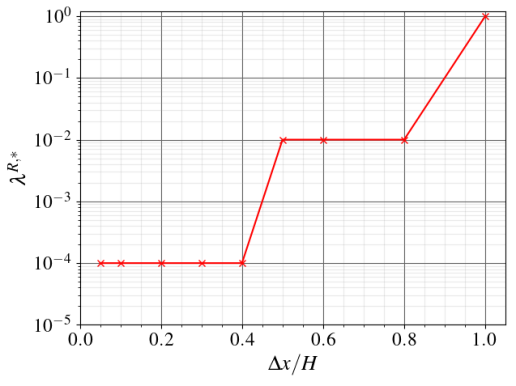
Figure 13: The optimised regularisation parameter, $\lambda^{R,*}$, with respect to data resolution.

B.2 Importance of regularisation for variational DA

For the variational DA, the choice of regularisation (of solenoidal forcing $f_{s,i}$) was more important. Three approaches were trialled: no regularisation; $L_{2}$ regularisation; $H_{1}$ regularisation.

		No Regularisation		$L_{2}$ Regularisation		$H_{1}$ Regularisation
	(a)		(b)		(c)
$U_{err}$
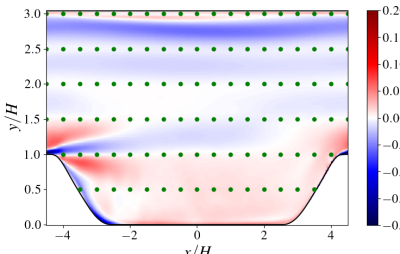
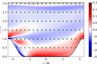
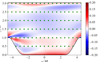
	(d)		(e)		(f)
$\left\|f_{s,i}\right\|$

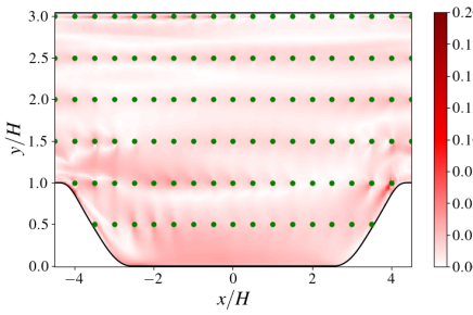
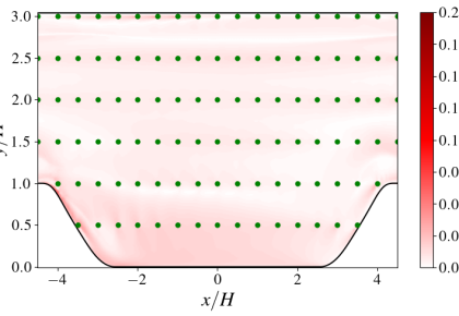
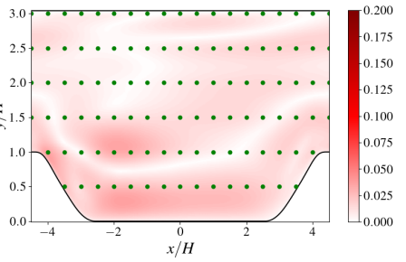
Figure 14: Absolute $U$ error (a,b,c) and corrective solenoidal forcing, $\left\|f_{s,i}\right\|$,(d,e,f) for variational-DA-SA method using different regularisation approaches: No regularisation (left), $L_{2}$ regularisation (middle) and $H_{1}$ regularisation (right).

Firstly, without regularisation, whilst data is well enforced (as seen in Figure 14(a) even compared with the final $H_{1}$ based approach, it results in a non-physical solenoidal forcing that appears strongly pointwise, clearly seen in Figure 14(d), as large corrections are applied at the data locations. The final reconstruction is thus less physical. Additionally, regularisation is needed to enforce convergence to a unique decomposition.

For the $L_{2}$ regularisation approach, error is higher than either $H_{1}$ or no regularisation methods. This is due to the inefficiency of the approach in the variational framework. To achieve sufficient smoothing of the solution, avoiding the problems of the none regularised approach, very large penalisation weighting is needing. However, this comes at the cost of poor data enforcement, as seen in Figure 14(b).

For the variational-DA-SA, $H_{1}$ regularisation was selected to smooth out the solution. As demonstrated, for the variational approach, $H_{1}$ regularisation is a much more suitable approach. It allows much better matching of the data (as compared with $L_{2}$ regularisation), whilst also giving a more physical solution. As a result this was selected as the final regularisation method.

For PINN-DA-SA, good data enforcement and a smooth non-pointwise solenoidal forcing was always ensured. Regularisation is exclusively used to control the distribution between modelled and corrective forcing. Given its computational simplicity, $L_{2}$ was selected for PINN-DA-SA. This was not the case for variational-DA-SA and regularisation was needed to smooth the solution in addition to the distribution of modelled and corrective forcing.

Appendix C Reconstructing pressure with PINN-DA-Baseline

Instead of applying the Helmholtz decomposition (4c) with the PINN-DA-Baseline, as in Section IV.2, one can alternatively enforce the base RANS equations as presented in (2b), using both high-fidelity first order statistics (mean flow) and second order statistics (Reynolds stress) ($U_{i},\overline{u_{i}^{\prime}u_{j}^{\prime}}$) at discrete locations to reconstruct the flow field. This approach enables reconstruction of both mean velocity and Reynolds stresses fields, but also allows the inference of the pressure field.

Table 2: Weights used in PINN optimisation when both mean velocity and Reynolds stress data are provided

Weight	$\lambda^{P}$	$\lambda^{D}(U_{i})$	$\lambda^{D}(\overline{u_{i}^{\prime}u_{j}^{\prime}})$	$\lambda^{B}(U_{i})$ - Wall	$\lambda^{B}(\overline{u_{i}^{\prime}u_{j}^{\prime}})$ - Wall	$\lambda^{B}$ - Periodic
Value	1	10	100	2.5	10	1

(a)

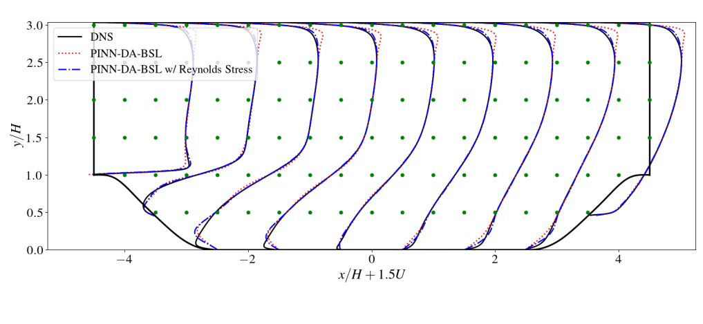
(b)      $\hat{P}$ (c) $P_{truth}$ (d) $P_{err}$

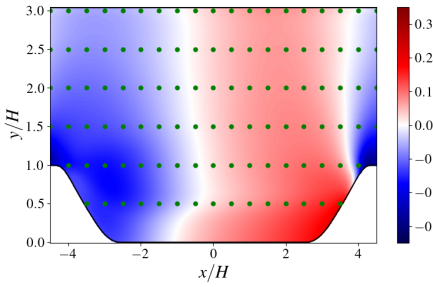
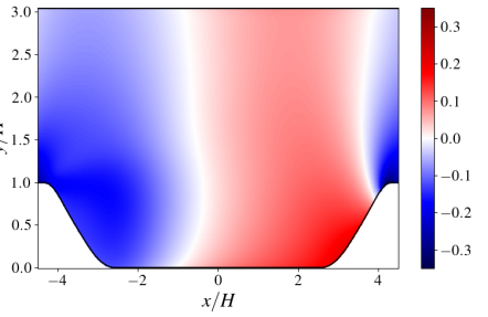
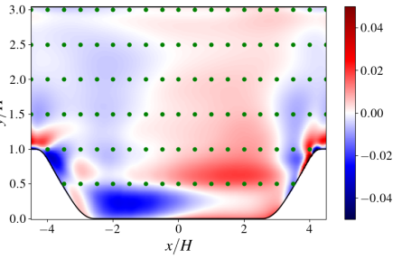
Figure 15: PINN-DA-Baseline mean flow reconstruction. (a) Comparison between the DNS, PINN-DA-Baseline and PINN-DA-Baseline (with Reynolds stress data) velocity profiles for the $U$ component. (b) Pressure field inferred from the PINN-DA-Baseline approach from sparse mean velocity and Reynolds stress data. (c) Absolute mean pressure error from PINN-DA-Baseline pressure reconstruction.

Using the data spacing $\Delta L=0.5$, shows that this alternate PINN-Baseline approach produces comparable mean velocity reconstruction as the PINN-DA-Baseline, as seen in Figure 15(a). The $L_{2}$ error is $3.37\times 10^{-2}$ for this second approach compared with $3.60\times 10^{-2}$ for the former approach. Likewise the key trends discussed in Section IV.2 all still hold. However, this alternate formulation has more output variables and fewer equations when compared to the approach used in the main paper.

Although both approaches achieve similar reconstruction error, this second approach requires second order statistics (Reynolds stress measurements) along with first order ones (mean flow field). However, this formulation can be used to reconstruct the pressure field, as shown before for laminar cases [31]. This is demonstrated in the turbulent case, as seen in Figure 15(b,c). This has a high potential for practical applications in order to obtain the pressure field without performing intrusive measurements. Examination of the RANS equations (2b) shows how provision of mean velocity and Reynolds stress data at discrete points defines all terms in the equations except for the pressure term. At these measurement locations, the equations are closed and the resultant neural network can infer a pressure field, both at data points but also away from them as well. This resultant pressure field has highest reconstruction error in the regions with highest pressure gradients in the flow, matching the trend seen with mean velocity error. The pressure reconstruction error is less correlated with the location of data points, than the mean velocity. It should be highlighted that the neural network pressure output must also include an integration constant (as the RANS equations only contain derivatives of pressure). To determine this constant and recover the actual, unshifted pressure field, one needs to fix the pressure at one point. This can be done during training (by providing pressure data at a single point) or as in this case, the pressure field is shifted in post processing. Taking the pressure data at a singular point, one can find a constant, such that by adding it to the model pressure at that point, the predicted pressure exactly matches the measurement. This constant can then be applied to the full solution.

Appendix D Laminar Cylinder Flow

	DNS
(a)

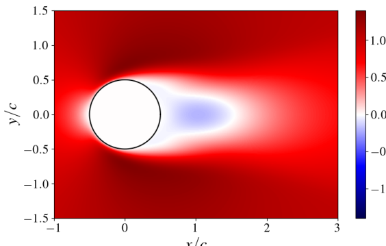
		Variational-DA		PINN-DA-Baseline
	(b)		(c)
$\hat{U}$
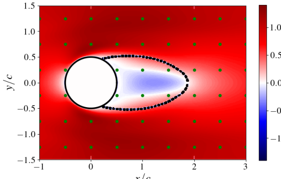
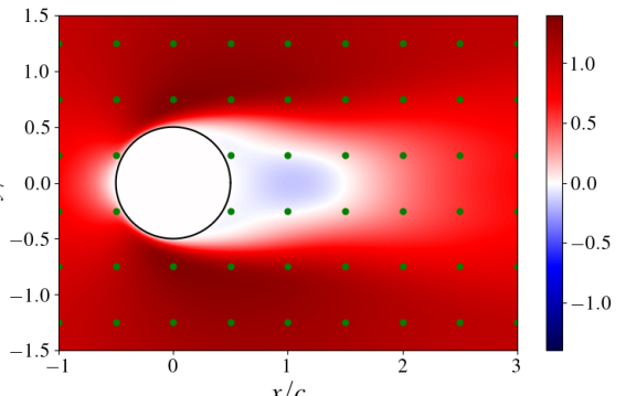
	(d)		(e)
$U_{err}$

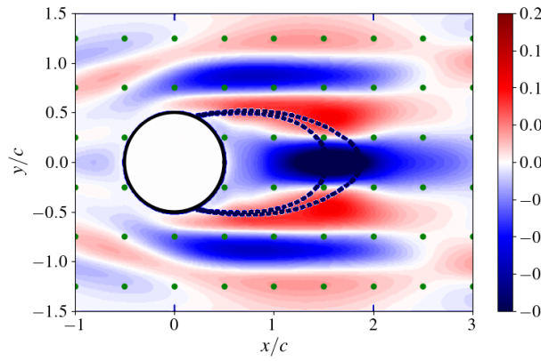
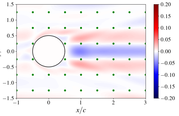
Figure 16: Comparison of the $U$ (x-component) mean velocity component reconstructions for $d=0.5$ data resolution with DNS (top). The variational-DA approach (left) and the PINN-DA-Baseline (right) figures are taken from [26] and [31] respectively. (a) - $U$ truth. (b,c) - $U$ prediction. (d,e) - Absolute $U$ error.

Both the variational-DA [26] and PINN-DA-Baseline [31] techniques (without the use of turbulence model augmentation) have already been successfully demonstrated on a laminar circular cylinder case. However, a quantitative comparison has not been completed, which is presented in this section.

A direct numerical simulation of a 2D circular cylinder flow at $Re=150$ is performed in order to generate the high fidelity database, which is used to extract sparse mean velocity measurements for use in the above data-driven techniques. The details of the simulation setup and methodologies can be found in  [26] and  [31] for the variational and PINN case respectively. Figure 16(a) shows the time-averaged mean $U$ field for the circular cylinder. For this work, the data spacing, $d=0.5$, on a rectangular grid is used to compare approaches as a comparison case. The aforementioned papers also contain results of differing data resolutions.

This direct comparison of both variational-DA and PINN-DA approaches was used as a benchmark for what the turbulent applications can achieve (as shown in the main paper). These results will demonstrate that for laminar flow, the PINN-DA approach flow reconstruction can match and improve the variational-DA reconstructions.

Figure 16 shows the reconstructed $U$ field (b,c) and the prediction error (d,e). This highlights several trends, which are consistent across all velocity components and were also seen in the turbulent cases. Firstly, the reconstructed mean velocity fields are very similar to the true fields and accurately capture the expected physical features, such as the symmetrical wake and the stagnation at the front of the cylinder. Additionally, a key pattern emerged from this result that was consistent across both the laminar and turbulent cases. Both the variational-DA and PINN-DA approaches have almost identical reconstruction error fields. These occur between datapoints, in the wake and recirculation regions and near the wall. Finally, as one moves away from the cylinder (in $y$), the error reduces as the flow becomes more uniform

Whilst the reconstruction error fields are comparable, it is clear that the absolute error for the PINN-DA-Baseline is much smaller in magnitude. The variational-DA has a maximum error magnitude of $0.3$ (for absolute $U$ error), whereas for PINN-DA it is around a third of this at $0.11$. This comparison is important as it suggests, all else equal for a laminar cylinder flow, the PINN-DA produces better results. This is most apparent when comparing the length of the wake. Whilst the variational approach predicts the wake recirculation region closes at $x=1.85$, the PINN approach closes at $x=1.55$ (compared with $x=1.55$ for the DNS flow field). Furthermore, the decay in error, observed as one moves away from the body, is much more apparent in the PINN-DA results. This may indicate the fundamental nature of PINNs and their construction, allows them to better generalise these simple uniform regions.

References

- Xiao and Cinnella [2019] H. Xiao and P. Cinnella, Quantification of model uncertainty in RANS simulations: A review, Progress in Aerospace Sciences 108, 1 (2019).
- Yarlanki et al. [2012] S. Yarlanki, B. Rajendran, and H. Hamann, Estimation of turbulence closure coefficients for data centers using machine learning algorithms, in 13th InterSociety Conference on Thermal and Thermomechanical Phenomena in Electronic Systems (IEEE, 2012) pp. 38–42.
- Zhang and Duraisamy [2015] Z. Zhang and K. Duraisamy, Machine learning methods for data-driven turbulence modeling, in 22nd AIAA computational fluid dynamics conference (2015) p. 2460.
- Ling et al. [2016] J. Ling, A. Kurzawski, and J. Templeton, Reynolds averaged turbulence modelling using deep neural networks with embedded invariance, Journal of Fluid Mechanics 807, 155 (2016).
- Spalart and Allmaras [1992] P. Spalart and S. Allmaras, A one-equation turbulence model for aerodynamic flows, in 30th aerospace sciences meeting and exhibit (1992) p. 439.
- Wilcox [1988] D. Wilcox, Reassessment of the scale-determining equation for advanced turbulence models, AIAA journal 26, 1299 (1988).
- Launder and Sharma [1974] B. Launder and B. Sharma, Application of the energy-dissipation model of turbulence to the calculation of flow near a spinning disc, Letters in heat and mass transfer 1, 131 (1974).
- Launder et al. [1975] B. Launder, G. Reece, and W. Rodi, Progress in the development of a Reynolds-stress turbulence closure, Journal of fluid mechanics 68, 537 (1975).
- Wallin and Johansson [2000] S. Wallin and A. Johansson, An explicit algebraic Reynolds stress model for incompressible and compressible turbulent flows, Journal of fluid mechanics 403, 89 (2000).
- Gatski and Speziale [1993] T. Gatski and C. Speziale, On explicit algebraic stress models for complex turbulent flows, Journal of fluid Mechanics 254, 59 (1993).
- Duraisamy et al. [2019] K. Duraisamy, G. Iaccarino, and H. Xiao, Turbulence modeling in the age of data, Annual Review of Fluid Mechanics 51, 357 (2019).
- Brunton et al. [2020] S. Brunton, B. Noack, and P. Koumoutsakos, Machine learning for fluid mechanics, Annual review of fluid mechanics 52, 477 (2020).
- Cherroud et al. [2022] S. Cherroud, X. Merle, P. Cinnella, and X. Gloerfelt, Sparse Bayesian Learning of Explicit Algebraic Reynolds-Stress models for turbulent separated flows, International Journal of Heat and Fluid Flow 98, 109047 (2022).
- Volpiani et al. [2021] P. Volpiani, M. Meyer, L. Franceschini, J. Dandois, F. Renac, E. Martin, O. Marquet, and D. Sipp, Machine learning-augmented turbulence modeling for RANS simulations of massively separated flows, Physical Review Fluids 6, 064607 (2021).
- Holland et al. [2019] J. Holland, J. Baeder, and K. Duraisamy, Towards integrated field inversion and machine learning with embedded neural networks for RANS modeling, in AIAA Scitech 2019 Forum (2019) p. 1884.
- Singh [2018] A. Singh, A framework to improve turbulence models using full-field inversion and machine learning, Ph.D. thesis (2018).
- Wu et al. [2019] J. Wu, H. Xiao, R. Sun, and Q. Wang, Reynolds-averaged Navier–Stokes equations with explicit data-driven Reynolds stress closure can be ill-conditioned, Journal of Fluid Mechanics 869, 553 (2019).
- Brener et al. [2021] B. Brener, M. Cruz, R. Thompson, and R. Anjos, Conditioning and accurate solutions of Reynolds average Navier–Stokes equations with data-driven turbulence closures, Journal of Fluid Mechanics 915 (2021).
- Edeling et al. [2014] W. Edeling, P. Cinnella, and R. Dwight, Predictive RANS simulations via Bayesian model-scenario averaging, Journal of Computational Physics 275, 65 (2014).
- Beetham and Capecelatro [2020] S. Beetham and J. Capecelatro, Formulating turbulence closures using sparse regression with embedded form invariance, Physical Review Fluids 5, 084611 (2020).
- Raissi et al. [2019] M. Raissi, P. Perdikaris, and G. Karniadakis, Physics-informed neural networks: A deep learning framework for solving forward and inverse problems involving nonlinear partial differential equations, Journal of Computational physics 378, 686 (2019).
- Eivazi et al. [2022] H. Eivazi, M. Tahani, P. Schlatter, and R. Vinuesa, Physics-informed neural networks for solving Reynolds-averaged Navier–Stokes equations, Physics of Fluids 34, 075117 (2022).
- Hasanuzzaman et al. [2023] G. Hasanuzzaman, H. Eivazi, S. Merbold, C. Egbers, and R. Vinuesa, Enhancement of PIV measurements via physics-informed neural networks, Measurement Science and Technology 34, 044002 (2023).
- Gao et al. [2021] H. Gao, L. Sun, and J. Wang, Super-resolution and denoising of fluid flow using physics-informed convolutional neural networks without high-resolution labels, Physics of Fluids 33, 073603 (2021).
- Kelshaw et al. [2022] D. Kelshaw, G. Rigas, and L. Magri, Physics-Informed CNNs for Super-Resolution of Sparse Observations on Dynamical Systems, arXiv preprint arXiv:2210.17319 (2022).
- Foures et al. [2014] D. Foures, N. Dovetta, D. Sipp, and P. Schmid, A data-assimilation method for Reynolds-averaged Navier–Stokes-driven mean flow reconstruction, Journal of fluid mechanics 759, 404 (2014).
- Symon et al. [2017] S. Symon, N. Dovetta, B. McKeon, D. Sipp, and P. Schmid, Data assimilation of mean velocity from 2D PIV measurements of flow over an idealized airfoil, Experiments in fluids 58, 1 (2017).
- Franceschini et al. [2020] L. Franceschini, D. Sipp, and O. Marquet, Mean-flow data assimilation based on minimal correction of turbulence models: Application to turbulent high Reynolds number backward-facing step, Physical Review Fluids 5, 094603 (2020).
- Symon et al. [2020] S. Symon, D. Sipp, P. Schmid, and B. McKeon, Mean and unsteady flow reconstruction using data-assimilation and resolvent analysis, AIAA Journal 58, 575 (2020).
- Agarwal et al. [2021] K. Agarwal, O. Ram, J. Wang, Y. Lu, and J. Katz, Reconstructing velocity and pressure from noisy sparse particle tracks using constrained cost minimization, Experiments in Fluids 62, 1 (2021).
- Sliwinski and Rigas [2022] L. Sliwinski and G. Rigas, Mean flow reconstruction of unsteady flows using Physics-Informed Neural Networks, Data-Centric Engineering 2021, 1 (2022).
- von Saldern et al. [2022] J. von Saldern, J. Reumschüssel, T. Kaiser, M. Sieber, and K. Oberleithner, Mean flow data assimilation based on physics-informed neural networks, Physics of Fluids 34, 115129 (2022).
- Molnar et al. [2023] J. Molnar, L. Venkatakrishnan, B. Schmidt, T. Sipkens, and S. Grauer, Estimating density, velocity, and pressure fields in supersonic flows using physics-informed BOS, Experiments in Fluids 64, 14 (2023).
- Du et al. [2023] Y. Du, M. Wang, and T. Zaki, State estimation in minimal turbulent channel flow: A comparative study of 4DVar and PINN, International Journal of Heat and Fluid Flow 99, 109073 (2023).
- Mons et al. [2022] V. Mons, O. Marquet, B. Leclaire, P. Cornic, and F. Champagnat, Dense velocity, pressure and Eulerian acceleration fields from single-instant scattered velocities through Navier–Stokes-based data assimilation, Measurement Science and Technology 33, 124004 (2022).
- Note [1] The data is available from https://github.com/xiaoh/para-database-for-PIML.
- Laizet and Li [2011] S. Laizet and N. Li, Incompact3d: A powerful tool to tackle turbulence problems with up to O (105) computational cores, International Journal for Numerical Methods in Fluids 67, 1735 (2011).
- Xiao et al. [2020] H. Xiao, J. Wu, S. Laizet, and L. Duan, Flows over periodic hills of parameterized geometries: A dataset for data-driven turbulence modeling from direct simulations, Computers & Fluids 200, 104431 (2020).
- Lu et al. [2021] L. Lu, X. Meng, Z. Mao, and G. Karniadakis, DeepXDE: A deep learning library for solving differential equations, SIAM Review 63, 208 (2021).
- Hecht [2012] F. Hecht, New development in FreeFem++, J. Numer. Math. 20, 251 (2012).
- Brooks and Hughes [1982] A. Brooks and T. Hughes, Streamline upwind/Petrov-Galerkin formulations for convection dominated flows with particular emphasis on the incompressible Navier-Stokes equations, Computer methods in applied mechanics and engineering 32, 199 (1982).
- Olshanskii et al. [2009] M. Olshanskii, G. Lube, T. Heister, and J. Löwe, Grad–div stabilization and subgrid pressure models for the incompressible Navier–Stokes equations, Computer Methods in Applied Mechanics and Engineering 198, 3975 (2009).
- Nocedal [1980] J. Nocedal, Updating Quasi-Newton Matrices With Limited Storage, Mathematics of Computation 35, 773 (1980).
- Wang et al. [2021] S. Wang, Y. Teng, and P. Perdikaris, Understanding and mitigating gradient flow pathologies in physics-informed neural networks, SIAM Journal on Scientific Computing 43, A3055 (2021).
- Van [2022] Optimally weighted loss functions for solving pdes with neural networks, author=van der Meer, R and Oosterlee, C W and Borovykh, A, Journal of Computational and Applied Mathematics 405, 113887 (2022).
- Zeng et al. [2022] Q. Zeng, S. Bryngelson, and F. Schäfer, Competitive Physics Informed Networks, arXiv preprint arXiv:2204.11144 (2022).