Chaos persists in large-scale multi-agent learning
despite adaptive learning rates

Abstract.

Multi-agent learning is intrinsically harder, more unstable and unpredictable than single agent optimization. For this reason, numerous specialized heuristics and techniques have been designed towards the goal of achieving convergence to equilibria in self-play. One such celebrated approach is the use of dynamically adaptive learning rates. Although such techniques are known to allow for improved convergence guarantees in small games, it has been much harder to analyze them in more relevant settings with large populations of agents. These settings are particularly hard as recent work has established that learning with fixed rates will become chaotic given large enough populations [17, 9]. In this work, we show that chaos persists in large population congestion games despite using adaptive learning rates even for the ubiquitous Multiplicative Weight Updates algorithm, even in the presence of only two strategies. At a technical level, due to the non-autonomous nature of the system, our approach goes beyond conventional period-three techniques [29] by studying fundamental properties of the dynamics including invariant sets, volume expansion and turbulent sets. We complement our theoretical insights with experiments showcasing that slight variations to system parameters lead to a wide variety of unpredictable behaviors.

1. Introduction

Arguably one of the most thorny problems on the intersection of learning and games is the development of simple and practical algorithms that converge to Nash equilibria. The problem in its full generality is known to be intractable [18, 23], however, recent developments in Machine Learning have lead to a revived interest in the problem even in special classes of games. Unfortunately, the additional scrutiny has only helped crystallize the severity of the problem at hand through a diverse set of non-convergence, instability results even in well motivated special classes of games [31, 5, 19, 2, 22, 28, 4, 24, 6, 7]. Worse yet, standard online learning meta-algorithms, such as Multiplicative Weights Updates (MWU), have been shown to exhibit chaos [33, 13, 14, 15, 9, 17], which has be shown to be rather common in more complex games, e.g., as we increase the number of agents  [21, 37, 9, 17]. Given this proliferation of negative results, what other approaches are left to explore?

An interesting hint can be found in some of the earliest AI work on the subject. [42] established arguably one of the first non-convergence results in the area, showing that gradient dynamics do not suffice to achieve point-wise convergence even in the trivial case of two agent, two strategy games. On the positive side, when those dynamics are non-convergent, time-average convergence results can be established. Building up on their work, [12] showed that a modification of these standard dynamics where the agents can dynamically update their step-size based on payoff cues from their environment suffices to stabilize these dynamics in all $2\times 2$ games. Informally, the specific heuristic, Win or Learn Fast (WoLF), has the agents increase their learning rate when they are "losing" in an effort to escape from a non-promising region of the state space. Unfortunately, WoLF requires that each agent has knowledge to a Nash equilibrium strategy for themselves, which means it can only be applied in small games. On the positive side, this first result has led to several other more similar heuristics, with promising results in small games [8, 11, 1, 25, 26, 10]. While staying in the realm of small games, such heuristics have been shown to robustly improve the stability of other popular learning heuristics such as Proximal Policy Optimization [38, 35]. On the negative side, even for slightly larger games most positive results are largely empirical in nature and effectively very little is known about the behavior of such techniques in games with many agents. These works raise our key motivating question:

Does the simple idea of judiciously increasing the learning rate to “escape" barren regions of the state space scale to games with a large number of agents? If not, what type of formal instability results can be established?

Our approach. We focus on one of the most well studied class of large population games, non-atomic congestion games [36, 32] where the agents learn using the ubiquitous MWU update rule [3, 20, 30]. Furthermore, given the recent works of [17, 9], we focus on games with exactly two strategies/routes and linear cost functions, since such settings are already sufficiently hard for dynamics. Specifically, given fixed, non-adaptive learning rates, MWU dynamics typically will bifurcate to chaotic behavior for a large enough population size. Critically, however, these previous results are based on the celebrated "Period three implies chaos" methodology pioneered by Li-Yorke [29], which is only applicable in autonomous, i.e., time-invariant systems. In contrast, understanding the emergent behavior in our case will require totally different techniques.

Our model will allow for a wide range of dynamically adaptive learning rates. In particular, instead of having only two learning rates, fast and slow, as, e.g., in [12], we will allow for a continuous range of learning rates. Moreover, the decision to increase/decrease the learning rate will be driven by a regret-like measure [39]. Intuitively, each agent compares the historical time-average performance of both routes available to them. If both routes appear very similar to each other then the agents favor large learning rates so as to reach sufficiently different configurations where they can hopefully find informative payoff signals to exploit. On the other hand, if one route is significantly better than the other then the agents will take smaller but non-vanishing step sizes so as to take advantage of such opportunities without overcorrecting.

Our main result. We prove that our class of dynamics exhibits Li-Yorke chaotic behavior, implying the existence of an uncountable set of initial conditions that become “scrambled" by the dynamics (Theorem 4). Formally, for any two initial conditions from this set, the trajectories of the game dynamics come arbitrarily close to each other and move away from each other infinitely often.

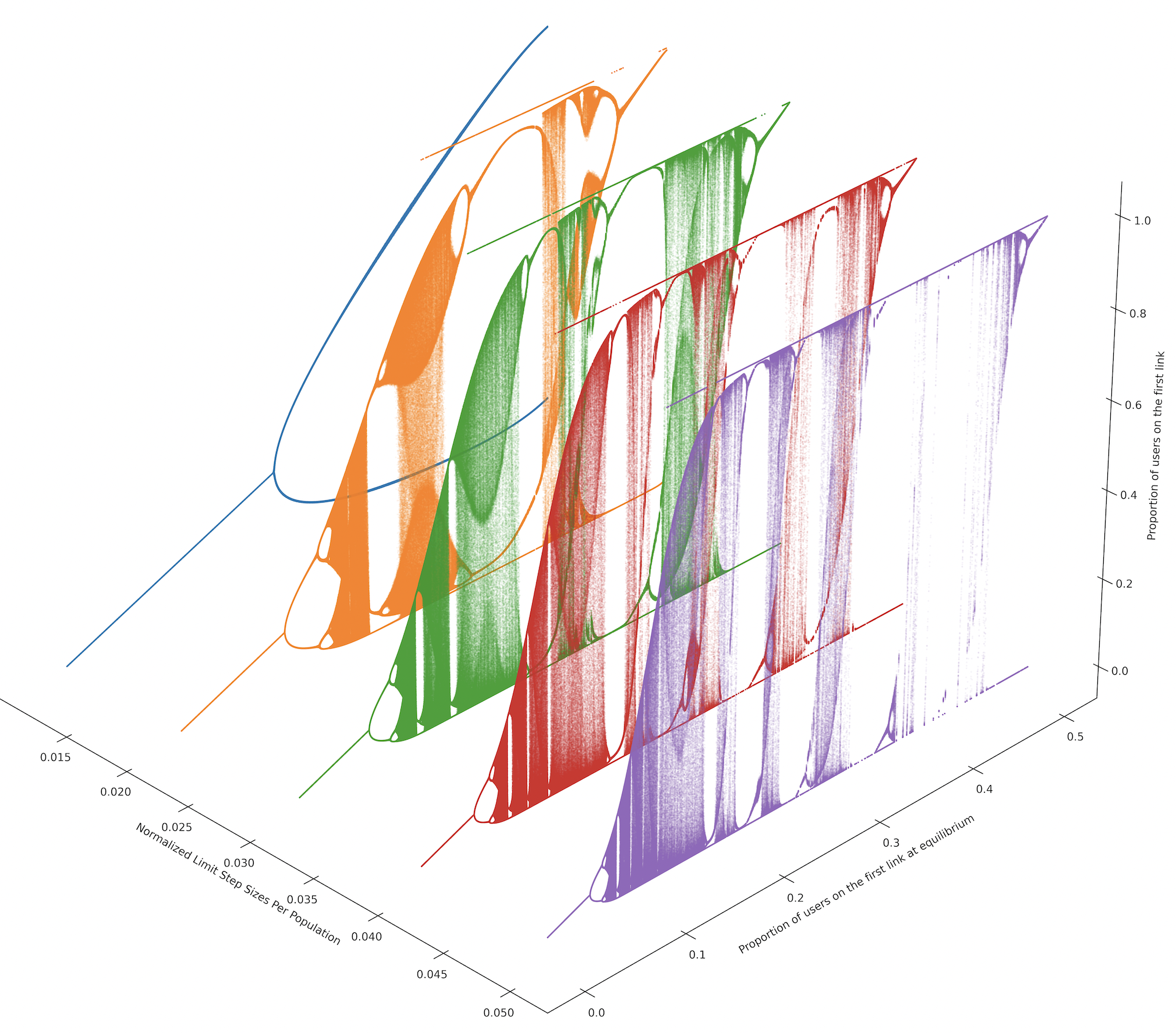
Figure 1. An assortment of bifurcation diagrams for different adaptive learning rate schemes. Larger volatility (larger limit step-size) leads to more prominently unpredictable, chaotic behavior (dense limit-sets for large fraction of the parameter space).

Our techniques. Despite the intense recent interest in developing formal arguments about chaos in game settings [9, 17, 27, 34] proving chaos in non-autonomous dynamical systems is a challenging endeavor, as the departure from one-dimensional autonomous systems gives up from many established equivalences among different notions of chaos, such as volume expansion, topological entropy, and arbitrarily long periodic points.

One possible approach to addressing this challenge would be to first establish that the sequence of employed maps converges uniformly to a fixed chaotic map, and then transfer the resulting scrambled set of the limit system to the non-autonomous one.

Although this property is not true for our system, it suffices to use a slightly relaxed version of it. We establish uniform convergence guarantees for initialization sets that are confined to the interior of the strategy space (Lemma 10), while tolerating the discrepancy between the varying-step and the corresponding MWU map in the limit. To confirm the existence of an uncountable scrambled set, we propose a novel connection between the behavior of MWU maps with varying learning rates and symbolic dynamics. Essentially, our proof strategy entails assigning every binary sequence to a different initialization such that scrambled binary strings correspond to scrambled initializations of the our non-autonomous dynamical system (Proof of Theorem 4).

The first part of our analysis (Section 3) involves enhancing previously existing results for the case of fixed learning rate dynamics. Specifically, we present an explicit construction of a perpetual set $\mathcal{F}(a)$, i.e., a forward invariant set where our dynamical system is surjective, $f_{a}(\mathcal{F}(a))=\mathcal{F}(a)$, where $f_{a}$ represents the MWU system with fixed learning rate $a$. (Lemma 3). Next we further show that, even in the presence of agent volatility due to their high learning rates, if their initial strategies lie within the interior of the strategy space, their strategies will eventually be absorbed into the perpetual set we have constructed (Lemma 4).

In the case of fixed learning rate, we are able to quantify an even stronger volume expansion result. Specifically, we show that the image of any arbitrarily small neighborhood of the mixed equilibrium of our game will converge exactly to the perpetual set we have constructed (Theorem 2).

Turning our attention to the adaptively dynamic learning rate (Section 4), we show that thanks to $\mathcal{F}(a)$, while learning rate may vary over iterations and initializations, there exists a set $\Delta$ –the closure of all perpetual sets $\mathcal{F}(a_{n})$ –to which our dynamics eventually will be absorbed (Lemmas 5,6), provided the initialization set lies in the interior of solution space. Leveraging this property, we show that despite the volatility due to agents employing potentially high learning rates, our average regret-like concepts converge for nearly all initial conditions (Lemmas 7,8,9). It is noteworthy that this result requires a substantial degree of additional technicality in contrast to its analogue for the fixed rate regime [17].

Before developing our machinery for the symbolic dynamics reduction in Section 5, our proof strategy includes an additional step of demonstrating that our system does not collapse early in any fixed point or subspace of strategies that lacks volume expansion, as this would eliminate chaos. To achieve this, we rely on Theorem 3 which guarantees that almost all neighborhoods of mixed equilibrium will avoid this scenario by volume expanding and approximately covering $\mathcal{F}(\displaystyle\lim_{n\to\infty}a_{n})$. Putting everything together our main result about chaotic limit behavior follows.

2. Problem setup and preliminaries

2.1. Dynamical systems & Li Yorke chaos

A discrete autonomous $m$-dimensional dynamical system is described by an equation $x_{n+1}=f(x_{n})$ for a function $f:\mathbb{R}^{m}\to\mathbb{R}^{m}$. In contrast a discrete $m$-dimensional non-autonomous dynamical system is described by an equation $x_{n+1}=f(x_{n},n)$ for a function $f:\mathbb{R}^{m}\times\mathbb{N}\to\mathbb{R}^{m}$. In both of these cases we can view the $x_{n}(x_{0})$ iterate as a function of the initialization $x_{0}$. We thus term the sequence $\{x_{n}(x_{0})\}_{n\in\mathbb{N}}$ the orbit of the dynamical system of $x_{0}$.

We call two initializations $p,q$ of a dynamical system scrambled if $\limsup_{n\to\infty}\|x_{n}(p)-x_{n}(q)\|>0$ and $\liminf_{n\to\infty}\|x_{n}(p)-x_{n}(q)\|=0$. Intuitively the orbits of $p,q$ continuously alternate between moving apart and arbitrarily close respectively. A set $S$ is scrambled if every pair $p,q\in S$ is scrambled. We are now ready to define the notion of Li Yorke chaos for both autonomous and non-autonomous dynamical systems.

Definition 1.

An autonomous/non-autonomous dynamical system is called Li Yorke chaotic if there is an uncountably infinite set $S$ that is scrambled.

A famous result for the case of one dimensional autonomous dynamical systems provides a simple and easily verified sufficient condition for chaos based on periodic orbits:

Theorem 1 ([29]).

Let $J$ be an interval and $f:J\to J$ be a continuous map of a dynamical system. If $f$ has a period-three orbit, then it is Li-Yorke chaotic.

2.2. Linear congestion games

In this work we consider the case of non-atomic two strategy linear congestion games. In a non-atomic congestion game, there is a continuum of agents each of which controls an infinitesimal fraction of the total flow $N$. In each iteration, a fraction of agents $x$ choose the first action and $1-x$ the second one, suffering costs $c_{1}(x)=\gamma Nx$ and $c_{2}(1-x)=\delta N(1-x)$ respectively where $\gamma,\delta>0$ are the linear cost coefficients of each action respectively.

2.3. Multiplicative Weights Update

The dynamics of the MWU meta-algorithm correspond to an autonomous dynamical system. Given the common learning rate of all agents $\eta>0$, the MWU update is as follows

$$x_{n+1}=\frac{x_{n}e^{-\eta c_{1}(x_{n})}}{x_{n}e^{-\eta c_{1}(x_{n})}+(1-x_{n})e^{-\eta c_{2}(1-x_{n})}}=\frac{x_{n}}{x_{n}+(1-x_{n})e^{-\eta(c_{2}(1-x_{n})-c_{1}(x_{n}))}}$$

We can further simplify the MWU update rule by making the following changes of variables

$$a=\frac{N\eta}{\delta+\gamma} b=\frac{\delta}{\delta+\gamma}$$

where $a$ corresponds to a normalized learning rate that accounts for the scale of $c_{1}$ and $c_{2}$ and $(b,1-b)$ is the Nash equilibrium of the game. The simplified update rule can be expressed via a parametric map $f$ over $a$ and $b$ that captures the whole class of games we are interested in

$$x_{n+1}=f(x_{n},a,b)=\frac{x_{n}}{x_{n}+(1-x_{n})\exp(a(x_{n}-b))}.$$ (1)

When $a,b$ are fixed we may skip them from the notation of MWU map and use just $f(x)$.

2.4. Dynamic Learning Rate Model

Here we extend the MWU meta-algorithm to adaptive learning rates $\eta$. The basis of our adapting dynamics is a notion of pseudo-regret that the agents suffer when choosing the first action over the second one. The definition captures the average difference of costs between the two actions weighted by the learning rate at each iteration $\eta_{i}$:

$$r_{n+1}=\frac{1}{n+1}\sum_{i=0}^{n}\eta_{i}[c_{1}(x_{i})-c_{2}(1-x_{i})].$$

Based on this calculation of pseudo-regret, the agents may seek to adapt their learning rates $\eta_{i}$ in order to balance between exploration and exploitation. When $|r_{n}|$ is big then it is clear than one action dominates over the other so the agents seek to move in the direction of improving costs but hopefully not too aggressively so as not to overshoot, akin to a gradient-like dynamics. In contrast, when $|r_{n}|$ is close to zero the average penalty of switching between actions is small since they suffer the same weighted cost in average. Thus there is an opportunity for the agents to increase their learning rate to encourage exploration while the cost differences are low. To hedge between exploration and exploitation as above, agents can pick appropriate function $h:\mathbb{R}\to\mathbb{R}^{+}$ that peaks at $0$ and setting $\eta_{n}=h(r_{n})$.

This dynamics of adapting $\eta_{i}$ to the pseudo-regret can be implemented as a 2-dimensional non-autonomous dynamical system with $x_{n}$ and $r_{n}$ as its state variables:

$$x_{n+1}=f\left(x_{n},\frac{Ng(r_{n})}{\gamma+\delta},b\right)\quad r_{n+1}=\frac{nr_{n}+h(r_{n})(c_{1}(x_{n})-c_{2}(1-x_{n}))}{n+1}.$$ (2)

The system is non-autonomous in the 2-dimensional space as the update rule of $r_{n}$ depends on $n$. We can always view $d$-dimensional non-autonomous systems as autonomous systems in $d+1$ dimensions by treating $n$ as an additional dimension. However, this does not really simplify things as Theorem 1 does not apply beyond a single dimension.

For simplicity, we rewrite the dynamics in terms of the normalized learning rates $a_{i}$. Let $a_{i}$ be the normalized learning rates corresponding to $\eta_{i}$ based on Eq. 1. We can then rewrite $r_{n+1}$ as

$$r_{n+1}=\frac{1}{n+1}\sum_{i=0}^{n}a_{i}[x_{i}-b].$$

Similarly, given that $\eta_{i}$ and $\alpha_{i}$ are equivalent up to game specific scale parameters, we can always find a $g$ such that $a_{n}=g(r_{n})$ . Instead of working in terms of the cumbersome dynamical system update rule Eq. 2, we will be be performing our analysis in terms of these simpler equations

$$x_{n+1}=f(x_{n},a_{n},b) a_{n+1}=g\left(\frac{\sum_{i=0}^{n}a_{i}(x_{i}-b)}{n+1}\right).$$

In the following sections we will make some assumptions on $g$. We will chose $g$ to be a continuous function bounded in $[a_{\min},a_{\max}]\subset\mathbb{R}^{+}$. We will also assume that the initialization $a_{0}$ is also a constant in $[a_{\min},a_{\max}]$.

Throughout this work we will think of $x_{n}$ and $a_{n}$ as functions of the initialization $x_{0},a_{0}$. Thus, the complete notation of the $n$-th iterate would be $x_{n}(x_{0},a_{0})$ and $a_{n}(x_{0},a_{0})$, however, when it does not hinder understanding we will drop the explicit description of all the dependencies.

3. Refinements in Fixed Learning rates

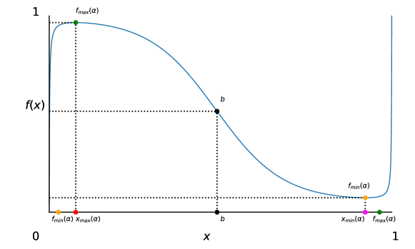
Figure 2. The order of $f_{min}(a)$, $x_{\max}(a)$, $b$, $x_{\min}(a)$, $f_{max}(a)$ in $x$-axis.

We start our analysis by providing a refined analysis in the regime of fixed learning rate as in [17]. In the following we will examine conditions of such systems under the assumption of $a>4$. Let us study the local minima and maxima of $f$:

$$x_{\min/\max}(a)=\frac{1}{2}\pm\sqrt{\frac{1}{4}-\frac{1}{a}}$$

Correspondingly we will denote $f_{\max}(a)=f(x_{\max}(a),a,b)$ and $f_{\min}(a)=f(x_{\min}(a),a,b)$. Our first observation is connected with the order of these values for high enough learning rate:

Lemma 1.

For every $b\in(0,1)$, there is a $a_{b}$ such that for all $a>a_{b}$

$$f_{\min}(a)<x_{\max}(a)<b<x_{\min}(a)<f_{\max}(a)$$

and $f_{\min}(a)$ is decreasing and $f_{\max}(a)$ is increasing.

Additionally, by construction, we can show that the interval $\mathcal{F}(a)=[f_{min}(a),f_{max}(a)]$ consists a forward invariant set for our dynamical system. In other words, if the MWU map with fixed learning rate $a$ starts in a state that is within $I$, it will remain in that set for all future times.

Lemma 2.

For every $b\in(0,1)$ there is a $s_{b}$ such that $\mathcal{F}(a)$ is forward invariant for all $a>s_{b}$, i.e.

$$x\in\mathcal{F}(a)\Rightarrow f(x,a,b)\in\mathcal{F}(a).$$

We can also prove that $f$ is surjective on $\mathcal{F}(a)$ for high enough learning rates.

Lemma 3.

For $a>a_{b}$, $f$ is surjective on $\mathcal{F}(a)$, i.e. $f(\mathcal{F}(a),a,b)=\mathcal{F}(a).$

When $\mathcal{F}(a)$ is both surjective and forward invariant as is the case for $a>a_{b},s_{b}$, we will call $\mathcal{F}(a)$ a perpetual set. Actually, $\mathcal{F}(a)$ is also an absorbing set for all $x\in(0,1)$, in the following sense:

Lemma 4.

Let $a>s_{b}$, $x_{0}\in[\gamma,\zeta]\Rightarrow\exists n_{0}:\ \forall n\geq n_{0}\text{ s.t }\ x_{n}\in\mathcal{F}(a)$, for every $[\gamma,\zeta]\subset(0,1)$.

We now turn to the chaotic properties of $f$. Given that period-three orbits do not carry over to the dynamic learning rate case, we choose to study an alternative property of chaotic maps, namely volume expansion. In autonomous maps, the existence of period-three orbits together with Theorem 1 imply that there is an initialization set whose volume under the dynamics expands quickly. Intuitively, the more volume this initialization set covers the more chaotic the dynamic is. While Theorem 1 guarantees the existence of volume expansion, it does not quantify how much volume it eventually covers. We prove that any interval around $b$ is sufficient to eventually cover $\mathcal{F}(a)$:

Theorem 2.

For every $b\in(0,1)$, there is a $v_{b}$ such that for all $a>v_{b}$ and any interval $[\gamma,\delta]$ : $\{b\}\subset[\gamma,\delta]\subset(0,1)$, it holds that

$$\exists n_{0}:\ \forall n\geq n_{0}\quad f^{n}([\gamma,\delta],a,b)=\mathcal{F}(a).$$

The proof of this theorem, which notably has not been established in any prior work, relies on a novel argument that is based on the monotonicity of $f$ on $\mathcal{D}=[x_{\max}(a),x_{\min}(a)]$, the lack of period-2 trajectories in $\mathcal{D}$ and the instability of fixed point $x=b$.

The key takeaway for the next section is that we can focus our efforts on analyzing the behavior of the non autonomous system in the interior of $(0,1)$ with special attention to neighborhoods of $b$ that alone can exhibit chaotic behavior. This is especially important because as we will see our notion of pseudo-regret converges uniformly in closed intervals in the interior of $(0,1)$ but not on $[0,1]$.

4. Chaos in Uniformly Convergent Non-autonomous Dynamical Systems

Turning our attention to the dynamic learning rate setting, we will refer to $x_{n}(x_{0})$ as the $n$-th iterate given the initialization $x_{0}$, and $a_{n}(x_{0})$ the learning rate at the same iteration, respectively.

Leveraging the existence of the perpetual set $\mathcal{F}(a)$ in the fixed rate case, we can construct a forward invariant absorbing set. This set will be crucial in proving the Li-Yorke chaotic behavior for the non-autonomous case. Intuitively, although the learning rate is varying both among different initializations and iterations, there exists a set which corresponds to the closure of all perpetual sets $\{\mathcal{F}(a_{n})\}$, to which our dynamics are always absorbed. This motivates the definition of set $\Delta$ as

$$\Delta=\left[\min_{a\in[a_{\min},a_{\max}]}f_{\min}(a),\max_{a\in[a_{\min},a_{\max}]}f_{\max}(a)\right]$$

where $a_{\min}$ and $a_{\max}$ are the $\min_{x_{0}\in[0,1]}g(x_{0})$ and $\max_{x_{0}\in[0,1]}g(x_{0})$ correspondingly.

Lemma 5 (Forward Invariance Property).

For all $a_{\min}>s_{b}$ we get that $\Delta$ is forward invariant, i.e.

$$x_{n}(x_{0})\in\Delta\implies x_{n+1}(x_{0})\in\Delta.$$

More interestingly, we show that eventually, any subinterval of $(0,1)$ will be absorbsed within $\Delta$.

Lemma 6 (Absorption Property).

For all $a_{\min}>s_{b}$ and $[\gamma,\zeta]\subset(0,1)$, there is an $n_{0}\geq 0$ so that

$$\forall n\geq n_{0}\quad x_{n}([\gamma,\zeta])\subseteq\Delta.$$

The key observation for the proof of the aforementioned lemmas is the fact that at any iteration $x_{n}(x_{0})$ will always come closer to the perpetual absorbing set $\mathcal{F}(a_{n}(x_{0}))$ and thus to its closure $\Delta$.

An immediate consequence of this lemma is the following corollary which will be dominant element for the uniform convergence both of our proposed pseudo-regret notion and the Césaro mean of the iterations. Analytically, for a given subinterval $[\gamma,\zeta]$ of $(0,1)$, we can always choose some $\delta>0$ such that $\Delta\cup[\gamma,\zeta]\subseteq(\delta,1-\delta)$. Again such choice of $\delta$ is possible because the attraction to $\Delta$ is not eventual phenomenon – at each iteration, $\mathrm{dist}(x_{n}(x_{0}),\Delta)$ will be either zero or always decreasing . This argumentation is expressed by the following statement:

Corollary 1.

Let $a_{\min}>s_{b}$, then for every $[\gamma,\zeta]\subset(0,1)$, there is an $\delta>0$ so that

$$\forall n\geq 0\quad x_{n}([\gamma,\zeta])\subseteq(\delta,1-\delta).$$

Having established Corollary 1, we are now in a position to present our claims regarding the average convergence for any initialization in $(0,1)$. Notably, while the individual iterates of the system, as we shall demonstrate in the ensuing section, exhibit chaotic characteristics, the iterate averages display stabilization over time.

Corollary 1 indicates that for any $x_{0}\in(0,1)$, $x_{n}(x_{0})$ will remain bounded away from the endpoints ${0,1}$. We now seek to connect how the boundness away from ${0,1}$ affects the average iterate of a trajectory. By induction on $x_{n+1}=f(x_{n},a_{n},b)$ we can prove the following

$$x_{n}=\frac{x_{0}}{x_{0}+(1-x_{0})\exp\left(\sum_{i=0}^{n-1}a_{i}(x_{i}-b)\right)}.$$ (3)

Observe that if we choose a $x_{0}\in(0,1)$, then $x_{n}$ is bounded away from ${0,1}$ if and only if $\sum_{i=0}^{n-1}a_{i}(x_{i}-b)$ is bounded. Specifically we can prove:

Lemma 7.

Let $a_{\min}>s_{b}$ and $x_{0}\in(0,1)$, then

$$\lim_{n\to\infty}\frac{1}{n+1}\sum_{i=0}^{n}a_{i}(x_{0})(x_{i}(x_{0})-b)=0.$$

Upon examination of the proof, a salient conclusion is that as $x_{0}$ moves farther away from the absorbing set $\Delta$ and closer to the endpoints ${0,1}$, the aforementioned convergence rate becomes increasingly slow, and fails in the case that $x_{0}\in\{0,1\}$, precluding a blanket result for the closed interval $[0,1]$. Conversely, if we restrict our attention to an arbitrary subinterval $[\gamma,\zeta]$, bounded away from the endpoints, we can always exploit the minimum convergence rate of this interval to derive a uniform convergence bound for the learning rate

Lemma 8.

Let $a_{\min}>s_{b}$. The sequence of functions $a_{n}(\cdot)$ is converging uniformly to the constant function $a^{\star}(\cdot)=g(0)$ in every interval $[\gamma,\zeta]\subset(0,1)$.

Having established that $a_{n}(x_{0})$ converges to $a^{\star}=g(0)$ for any $x_{0}\in(0,1)$, we are able to strengthen Lemma 7, demonstrating that its unweighted version of the Césaro mean (i.e. the average iterate in the limit of infinite time) also converges to $b$.

Lemma 9.

Let $a_{\min}>s_{b}$ and $x_{0}\in(0,1)$, then

$$\lim_{n\to\infty}\frac{1}{n+1}\sum_{i=0}^{n}x_{i}(x_{0})=b.$$

It is noteworthy that, despite this being equivalent to the guarantee provided in prior work, e.g. [17], for the fixed learning rate case, the machinery developed here for the adaptive rate regime has been more complex and involved.

The next lemma will be essential in our proofs of chaos and examines the relationship between $(x_{n}(x_{0}),a_{n}(x_{0}))$ and the MWU map with a fixed learning rate $f(x_{n}(x_{0}),a^{\star},b)$.

Lemma 10.

Let $a_{\min}>s_{b}$. For every $k$, $\epsilon>0$ and $[\gamma,\zeta]\subset(0,1)$

$$\exists n_{0}:\forall n\geq n_{0}\ \max_{x_{0}\in[\gamma,\zeta]}\lvert x_{n+k}(x_{0})-f^{k}(x_{n}(x_{0}),a^{\star},b)\rvert\leq\epsilon.$$

We can intuitively think of this result as a form of uniform convergence result for the sequence of MWU maps with varying learning rates to the fixed learning rate map. We establish this result by showing that for small changes in the learning rate, i.e., $a\in(a_{n}(x_{0})-\tilde{\epsilon},a_{n}(x_{0})+\tilde{\epsilon})$, the sensitivity of $f(x_{n}(x_{0}),a,b)$ is independent of the choice of $x_{0}$. It is thus not sufficient to prove that $f(x,a,b)$ is continuous in $a$. Instead we use the Mean Value Theorem to argue that $f(x,a,b)$ is Lipschitz continuous in $a$ with a Lipschitz constant independent of $x$. It is crucial to note that this uniform convergence result holds only in intervals $[\gamma,\zeta]\subset(0,1)$ because only then does the learning rate $a_{n}$ converge uniformly to $a(\cdot)=a^{\star}$.

We now prove our first volume expansion lemma for the dynamic learning rate case, namely that neighborhoods of $b$ within $\mathcal{D}(a_{\min})$ eventually expand to at least $\mathcal{F}(a_{\min})$. The intuition behind this result is based on the monotonicity property of $\mathcal{F}(a)$. Specifically, for high enough learning rates $a_{1}\leq a_{2}$, we have that $\mathcal{F}(a_{1})\subseteq\mathcal{F}(a_{2})$.

Lemma 11.

For every $b\in(0,1)$, there is an $z_{b}$ such that for all $a_{\min}>z_{b}$ it holds that for every $[\gamma,\delta]$ such that $\{b\}\subset[\gamma,\delta]\subseteq\mathcal{D}(a_{\min})=[x_{\max}(a_{\min}),x_{\min}(a_{\min})]$

$$\exists n_{0}:\ \forall n\geq n_{0}\ \ x_{n}([\gamma,\delta])\supseteq\mathcal{F}(a_{\min}).$$

Remark 1.

It is worth mentioning that the series of Lemmas 6,5,7 and 9,11 of this section –pertaining to forward invariance, absorption, volume expansion, and convergence of Césaro means –hold actually regardless of the choice of the update rule and are of independent interest.

For the case of the fixed learning rate, Theorem 2 makes a more refined prediction compared to Lemma 11 as the former provides an equality. In the dynamic learning rate case there is a gap between the eventual image upper bound, $\Delta$ and the volume expansion lower bound $\mathcal{F}(a_{\min})$. In order to close this gap we will make use of the fact that the learning rate converges to $g(0)$.

Building upon the full range of the developed machinery of this section, we will strengthen the above volume expansion result by showing that $a_{\min}$ could be actually substituted by any $\tilde{a}=a^{\star}-\epsilon$ for any sufficient small $\epsilon>0$ such that $a^{\star}-\epsilon>a_{\min}>z_{b}$. Our first observation is that thanks to the uniform convergence of $a_{n}\to a^{\star}$ in $[\gamma,\delta]\subset(0,1)$ there exists a $n^{{\dagger}}$ such that

$$\forall n>n^{{\dagger}}\quad\forall x\in[\gamma,\delta]\quad a_{n}(x)>a^{\star}-\epsilon=\tilde{a}$$

This strengthens the previous volume expansion result to at least the set $\mathcal{F}(\tilde{a})$ for any $\tilde{a}$ close to $a^{\star}$.

Theorem 3.

For $a_{\min}>z_{b}$ and for any sufficient small $\epsilon>0$ such that $a^{\star}-\epsilon>a_{\min}>z_{b}$ we have that for all $[\gamma,\delta]$ such that $\{b\}\subset[\gamma,\delta]\subset(0,1)$, it holds that

$$\exists n_{0}:\ \forall n\geq n_{0}\quad x_{n}([\gamma,\delta])\supseteq\mathcal{F}(a^{\star}-\epsilon).$$

In a completely similar fashion we can show that the absorbing set $\Delta$ can also be refined. For a given interval $[\gamma,\delta]\subset(0,1)$, as the learning rates converge to $a^{*}$, the trajectories will tend to be absorbed by $\mathcal{F}(a^{\star})$. Thus the dynamic learning rate volume expansion behavior matches fixed learning rate case in the long run.

5. Turbulent Sets and Chaos in MWU map

The roadmap of this section is our construction of the turbulent sets and their connection with the symbolic dynamics in order to prove Li-Yorke chaos in our non-autonomous dynamical system. It should be noticed that our novel approach is a major departure from the standard techniques of 3-period orbit arguments that have been extensively used in the case of fixed learning rates.

We start with some useful definition for our reduction.

Definition 2 ([40]).

A continuous map $f:I\to I$ is called turbulent if there exist compact subintervals $J,K$ with at most one common point such that $J\cup K\subseteq f(J)\cap J(K)$ Additionally, the map is called strictly turbulent if the subintervals can be chosen to be disjoint. Finally, the corresponding set $J,K$ are called turbulent sets.

Delving into the proof of [29], it becomes clear that the chaotic map $f(x,a,b)$ has a periodic orbit of period 3 that exists within the interior of $\mathcal{F}(a)$. We take advantage of this property to demonstrate that $f^{2}(\cdot,a,b)$ is in fact a strictly turbulent map.

Lemma 12.

For every $b\in(0,1)$, there is a $u_{b}$ such that for all $a>u_{b}$, there exist closed and disjoint intervals $K_{a}$ and $J_{a}$ in the interior of $\mathcal{F}(a)$ such that $f^{2}(K_{a},a,b)$ and $f^{2}(J_{a},a,b)$ are neighborhoods of $K_{a}\cup J_{a}$.

We begin by examining the properties of a fixed learning rate MWU map and its ability to create exponential decaying volume (length) turbulent sets. Our analysis centers around the key observation that since $f^{2}(K_{a})$ covers $K_{a}\cup J_{a}$, then there exist necessarily, by continuity of $f^{2}$, at least two distinct subintervals, $Z_{1},Z_{2}$, within $K_{a}$ whose $f^{2}$-image is precisely $K_{a}$ and $J_{a}$, respectively. By repeatedly applying this principle, we demonstrate that the $f^{4}$-image of these subintervals cover again $K_{a}\cup J_{a}$, and through induction, we can extend this property to higher compositions of $f$.

Lemma 13.

For every $a>u_{b}$, there exist closed intervals $V_{a}^{k}\subseteq K_{a}$ and $U_{a}^{k}\subseteq J_{a}$ such that

$$\lim_{k\to\infty}\textrm{diam}(V_{a}^{k})=\lim_{k\to\infty}\textrm{diam}(U_{a}^{k})=0$$

and for every $k\geq 0$ it holds that $f^{2k+2}(V_{a}^{k},a,b)$ and $f^{2k+2}(U_{a}^{k},a,b)$ are neighborhoods of $K_{a}\cup J_{a}$.

Figure 3. Illustration of the inductive construction of $V_{a}^{k}$ sets. In order to construct an exponential decaying sequence, we choose as $V_{a}^{1}=\arg\min_{Z\in\{Z_{1},Z_{2}\}}\textrm{diam}(Z)\leq\textrm{diam}(V_{a}^{0}=K_{a})$.

The following lemma plays an essential role in our symbolic dynamic proof of the Li-Yorke chaotic behavior. It allows us to construct a scrambled set of initial conditions through a set of abstract symbolic orbits.

On a technical level, we utilize a range of machinery developed in this paper to prove this lemma. Specifically, we use Theorem 3 to firstly describe turbulent sets $J_{a^{\star}}\cup K_{a^{\star}}$ that lie within the interior of $\mathcal{F}(a^{\star})$ and, for small enough $\epsilon$, within $\mathcal{F}(a^{\star}-\epsilon)$, and secondly to ensure that the non-autonomous dynamical system covers $J_{a^{\star}}\cup K_{a^{\star}}$. Furthermore, to extend the implication of Lemma 13 for the turbulent map $f^{2}(\cdot,a^{\star},b)$ to the non-autonomous system $x_{n}$ map for the sets $J_{a^{\star}},K_{a^{\star}}$, we employ the uniform convergence guarantee provided by Lemma 10, which controls the discrepancy between $x_{n+2}(S)$ and $f^{2}(x_{n}(S),a^{\star},b)$ for any subinterval $S$ of $J_{a^{\star}},K_{a^{\star}}$.

Lemma 14 (Tracking Lemma).

If $b\in(0,1)\setminus\{\frac{1}{2}\}$, there exists a $d_{b}$ such that if $a_{\min}>d_{b}$, we can construct an increasing sequence $n_{i}$ with the following properties. For every sequence of intervals $A_{i}$ with $A_{i}=V_{a^{*}}^{i}$ or $A_{i}=U_{a^{*}}^{i}$, there exists a $x_{0}\in[0,1]$ such that for all $i\geq 0$ it holds that $x_{n_{i}}(x_{0})\in A_{i}$ .

It is important to note that Lemma 14 ensures the ability to construct the same sequence of $n_{i}$ for any distinct sequence of $A_{i}$. Our approach to demonstrate the Li-Yorke chaotic behavior through symbolic dynamics is summarized in the following high-level steps:

• Assume that we can construct an uncountable set $\mathcal{S}$ of scrambled infinite length binary sequences, i.e., for every pair of sequences $\sigma,\tau\in\mathcal{S}$ there exist $(i)$ an infinite length subsequence $(k_{i})_{i\in\mathbb{N}}$ where the two sequences differ, i.e., $\sigma_{k_{i}}\neq\tau_{k_{i}}$ and $(ii)$ an infinite length subsequence $(\ell_{i})_{i\in\mathbb{N}}$ where the two sequences are equal, i.e., $\sigma_{\ell_{i}}=\tau_{\ell_{i}}$.

• For each element of $\sigma\in\mathcal{S}$ we construct a sequence of sets $\mathcal{A}_{\sigma}=(A_{i})_{i\in\mathbb{N}}$ as follows: If the $k$-th place element is $0$ we use $V_{a^{*}}^{k}$, whereas if it is $1$ we pick $U_{a^{*}}^{k}$. We now apply Lemma 14 for each of the sequence of sets to get a corresponding initialization $x_{0}^{\sigma}$. We call this set of initializations $Q$.

• Since every pair of strings $\sigma,\tau$ is scrambled, we know that we can construct two infinite subsequences $(\mu_{i})_{i\in\mathbb{N}},(\nu_{i})_{i\in\mathbb{N}}$ such that $\{x_{\mu_{i}}(x_{0}^{\sigma})\}$, $\{x_{\mu_{i}}(x_{0}^{\tau})\}$ belong to the same turbulent sets and $\{x_{\nu_{i}}(x_{0}^{\sigma})\}$, $\{x_{\nu_{i}}(x_{0}^{\tau})\}$ belong to the disjoint turbulent ones. Therefore, we can show that for every pair $\sigma,\tau\in Q$: $(i)\liminf\|\{x_{n}(x_{0}^{\sigma})-x_{n}(x_{0}^{\tau})\}\|=0\quad(ii)\limsup\|\{x_{n}(x_{0}^{\sigma})-x_{n}(x_{0}^{\tau})\}\|>0$

Formalizing the outlined proof sketch, our final result follows:

Theorem 4.

If $b\in(0,1)\setminus\{\frac{1}{2}\}$, there exists a $d_{b}$ such that if $a_{\min}>d_{b}$, the dynamics of Equation 2 are Li-Yorke chaotic.

In this work we have focused on the dynamics of Eq. 2. But our proof strategy can be readily generalized to any rule $a_{n}(\cdot)$ as long as it uniformly converges to a sufficiently high constant rate.

Corollary 2.

Let $a_{n}(\cdot)$ be a sequence of maps uniformly converging in $[0,1]$ to $a^{*}>d_{b}$. Then the resulting dynamic learning rate system is Li-Yorke chaotic.

6. Conclusion

We have formally analyzed and established chaotic behavior for a class of multi-agent learning systems with a heuristically updated, variable learning rate. At the technical crux of all prior formal analysis of Li-Yorke chaos in games (e.g., [9, 17, 27, 16, 34]) lied the celebrated methodology based on period three orbits [29], which is only applicable in autonomous, i.e., time-invariant systems. In contrast, we had to delve deeper into the geometry and structural properties of these dynamics, which itself evolve with time showing that formal analysis of chaos is still possible. This opens the possibility of extending prior results to more realistic time-varying models.

Appendix A Omitted Proofs of Section 3

In this section we will focus on the case where the dynamical system has a fixed learning rate.

$$x_{n+1}=f(x_{n},a,b)=\frac{x_{n}}{x_{n}+(1-x_{n})\exp(a(x_{n}-b))}$$

The derivative of $f$ for a fixed $a$ and $b$ is

$$f^{\prime}(x,a,b)=\frac{(ax^{2}-ax+1)\exp(a(x-b))}{(x+(1-x)\exp(a(x-b)))^{2}}$$

Critical/stationary points of $f$ are solutions of $ax^{2}-ax+1=0$. By taking the determinant, we get than for $0<a\leq 4$, there is no solution so $f$ is increasing and no chaos can exist, instead the system converges to equilibrium. We will thus require $a>4$ to enable chaotic behaviour in the system. Let us study the local minima and maxima of $f$:

$$x_{\max}(a)=\frac{1}{2}-\sqrt{\frac{1}{4}-\frac{1}{a}}\quad x_{\min}(a)=\frac{1}{2}+\sqrt{\frac{1}{4}-\frac{1}{a}}$$

A.1. The order of $\{f_{min}(a),x_{\max}(a),b,x_{\min}(a),f_{max}(a)\}$ in the fixed learning rate regime.

The following facts establish the preliminary necessary observation to prove structural Lemma 1. More precisely, we can show the following straightforward facts:

Fact A.1.

For every $b\in(0,1)$, there is a $s_{b}>4$ such that for all $a>s_{b}$

$$x_{\max}(a)<b<x_{\min}(a).$$

Proof.

We have $x_{\max}(a)$ is decreasing and $\lim_{a\to\infty}x_{\max}(a)=0$. Symmetrically we have $x_{\min}(a)$ is increasing and $\lim_{a\to\infty}x_{\min}(a)=1$. The fact follows immediately. ∎

Fact A.2.

If $a>4$, then $f(x_{\min}(a),a,b)=f_{\min}(a)<f(x_{\max}(a),a,b)=f_{\max}(a)$.

Proof.

Since the function is decreasing after the local maximum and there is no stationary point until the local minimum, the local minimum has smaller value. ∎

Fact A.3.

If $a>s_{b}$, then $f_{\min}(a)<b<f_{\max}(a)$.

Proof.

For $a>s_{b}$ we know that $f_{\min}(a)<f(b,a,b)=b$ since $f$ is decreasing in $[b,x_{\min}(a)]$. Symmetrically, $f_{\max}(a)>f(b,a,b)=b$ since again $f$ is decreasing in $[x_{\max}(a),b]$. ∎

Having presented the aforementioned intuitive facts, we are ready to prove Lemma 1

Lemma A.1.

[Restate Lemma 1] For every $b\in(0,1)$, there is a $a_{b}$ such that for all $a>a_{b}$

$$f_{min}(a)<x_{\max}(a)<b<x_{\min}(a)<f_{max}(a)$$

and $f_{\min}(a)$ is decreasing and $f_{\max}(a)$ is increasing.

Proof.

$f_{min}(a)<x_{\max}(a)$ is equivalent to

$$x_{\min}(a)-x_{\min}(a)x_{\max}(a)-x_{\max}^{2}(a)\exp\left[\alpha(x_{\min}(a)-b)\right]<0$$

Observe that the first two terms are bounded and that for the third term we have

$$\lim_{a\to\infty}x_{\max}^{2}(a)\exp\left[\alpha(x_{\min}(a)-b)\right]=\infty$$

So we can pick an $a_{b}$ large enough so that $a>a_{b}$ implies that the inequality holds. The case of $x_{\min}(a)<f_{max}(a)$ is symmetric. Moving on to the monotonicity of $f_{\min}(a)$, to avoid overloading notation let us call $x_{1}$ the $x$ argument of $f$ and $x_{2}$ its $a$ argument

$$\frac{\partial f_{\min}(a)}{\partial a}=\frac{\partial f(x_{\min}(a),a,b)}{\partial x_{1}}\frac{\partial x_{\min}(a)}{\partial a}+\frac{\partial f(x_{\min}(a),a,b)}{\partial x_{2}}$$

Observe that since $x_{\min}(a)$ is a local minimum, we have that

$$\frac{\partial f(x_{\min}(a),a,b)}{\partial x_{1}}=0$$

Additionally we can pick $a_{b}$ large enough so that $a>a_{b}$ implies $x_{\min}(a)>b$. Let us write $f(x_{\min}(a),a,b)$

$$f(x_{\min}(a),a,b)=\frac{x_{\min}(a)}{x_{\min}(a)+(1-x_{\min}(a))\exp(a(x_{\min}(a)-b))}.$$

Treating $x_{\min}(a)$ as a constant independent of $a$, the exponential in the denominator is an increasing function of $a$ so $f(x_{\min}(a),a,b)$ is decreasing with respect to $a$. This makes

$$\forall a>a_{b}\quad\frac{\partial f(x_{\min}(a),a,b)}{\partial x_{2}}<0$$

As a result we have that

$$\forall a>a_{b}\quad\frac{\partial f_{\min}(a)}{\partial a}<0$$ (A.1)

and $f_{\min}(a)$ is decreasing. The case of $f_{\max}(a)$ is symmetric. We take the maximum of all the required $a_{b}$ to get the result. ∎

A.2. Forward invariant, Perpetual & Absorbing sets for fixed learning rate.

Having settled the order among $\{f_{min}(a),x_{\max}(a),b,x_{\min}(a),f_{max}(a)\}$ for high enough learning rates, we are ready to prove the $(i)$ forward invariant, $(ii)$ perpetual and $(iii)$ absorbing property of $\mathcal{F}(a)=[f_{\min}(a),f_{\max}(a)]$.

For the sake of readability, we recall first the formal definitions of these properties:

1. A forward invariant set: a set of states such that if the system starts in any state in the set, it will remain in the set for all future time.

2. A perpetual set: a special case of a forward invariant set, whose image consists itself.

3. An (global/local) absorbing set: a forward invariant set that also includes (globally/locally) all possible future states of the system.

Lemma A.2.

[Restated Lemma 2] For every $b\in(0,1)$ there is a $s_{b}$ such that $\mathcal{F}(a)$ is forward invariant for all $a>s_{b}$, i.e.

$$x\in\mathcal{F}(a)\Rightarrow f(x,a,b)\in\mathcal{F}(a).$$

Proof.

By continuity of $f$, we only need to consider four points to determine the image of $[f_{\min}(a),f_{\max}(a)]$: $f_{\min}(a)$, $f_{\max}(a)$ as well as $x_{\max}(a)$, $x_{\min}(a)$. Since $f(x,a,b)\geq x$ in $(0,b)$ and $f_{\max}(a)$ is the maximum in this interval, we know that

$$f_{\max}(a)\geq f(f_{\min}(a),a,b)\geq f_{\min}(a)$$

Since $f(x,a,b)\leq x$ in $(b,1)$ and $f_{\min}(a)$ is the minimum in this interval, we know that

$$f_{\max}(a)\geq f(f_{\max}(a),a,b)\geq f_{\min}(a)$$

Of course the images of the local optima $x_{\max}(a)$, $x_{\min}(a)$ trivially belong to $[f_{\min}(a),f_{\max}(a)]$. ∎

But even points that are outside of this interval are monotonically attracted to it without overshooting. We have the following lemma that shows this monotic attracting property

Lemma A.3.

Let $a>s_{b}$, then

$$x\in(0,f_{\min}(a)) \implies f(x,a,b)\in(x,f_{\max}(a)]$$

$$x\in(f_{\max}(a),1) \implies f(x,a,b)\in[f_{\min}(a),x).$$

Proof.

We will prove the first one, the second one is entirely symmetric. If $x<f_{\min}(a)$ then $x<b$ and thus $f(x,a,b)>x$ and $f(x,a,b)\leq f_{\max}(a)$. The first implication follows immediately. ∎

Consequently, we have the following lemma:

Lemma A.4 (Restated Lemma 3).

For $a>a_{b}$, $\mathcal{F}(a)$ is surjective, i.e. $f(\mathcal{F}(a),a,b)=\mathcal{F}(a).$

Proof.

We already know that the right hand side is a super set of the left hand side by Lemma A.2. But by Lemma A.1 we have that $x_{\max}(a)$ and $x_{\min}(a)$ belong to $[f_{\min}(a),f_{\max}(a)]$. So the left hand is a super set of the left hand side. Thus the result follows. ∎

More generally we can prove the following absorbing condition:

Lemma A.5 (Restated Lemma 4).

Let $a>s_{b}$, $x_{0}\in[\gamma,\zeta]\Rightarrow\exists n_{0}:\ \forall n\geq n_{0}\text{ s.t }\ x_{n}\in\mathcal{F}(a)$, for every $[\gamma,\zeta]\subset(0,1)$.

Proof.

If $x_{0}\in[f_{\min}(a),f_{\max}(a)]$ then the results follows trivially for $n_{0}=0$. Let us take the case

$$x_{0}\in\left[\gamma,f_{\min}(a)\right)=\Delta_{0}$$

We know that in $\Delta_{0}$ we have that $f(x,a,b)>x$. We can define a uniform bound on their difference

$$\min_{x\in\Delta_{0}}\left[f(x,a,b)-x\right]=\xi>0$$

We now know that

$$x_{1}\in\left[\gamma+\xi,f_{\max}(a)\right)$$

If $x_{1}\in\Delta$ then the result follows trivially for $n_{0}=1$. Otherwise we have that

$$x_{1}\in\left[\gamma+\xi,f_{\min}(a)\right)\subset\Delta_{0}$$

Applying recursively, either there is a $n_{0}$ such that $x_{n_{0}}\in\Delta$ and the theorem follows trivially or for all $n$ we have that $x_{n}$ stays in a subset of $\Delta_{0}$

$$x_{n}\in\left[\gamma+n\xi,f_{\min}(a)\right)\subset\Delta_{0}$$

But this is impossible since there is a $n_{0}>0$ such that

$$\forall n\geq n_{0}:\gamma+n\xi>f_{\min}(a)$$

We are now left with the symmetric case of

$$x_{0}\in\left(f_{\max}(a),\zeta\right]$$

which we can handle just like above. ∎

A.3. Two period trajectories in MWU maps.

We start with a fundamental observation from Calculus of continuous injective function

Claim 1.

Let $g$ be a continuous decreasing function on a closed interval $I$ and that there exists a $x_{0}\in I$ such that $\forall n:g^{n}(x_{0})\in I$. Then either $g^{n}(x_{0})$ converges to a fixed point $x^{\star}$ or to a 2-period trajectory.

Proof.

Let us take $g^{n_{j}}(x_{0})$ a subsequence that converges to $\liminf_{n\to\infty}g^{n}(x_{0})$.

$$\limsup_{n\to\infty}g^{n}(x_{0})\geq\lim_{j\to\infty}g^{n_{j}+1}(x_{0})=g(\liminf_{n\to\infty}g^{n}(x_{0}))$$

Now let us take $g^{n_{k}}(x_{0})$ a subsequence that converges to $\limsup_{n\to\infty}g^{n}(x_{0})$. Since $g$ is decreasing and thus invertible in $I$ we know that $g^{n_{k}-1}(x_{0})$ also converges

$$\limsup_{n\to\infty}g^{n}(x_{0})=g(\lim_{k\to\infty}g^{n_{k}-1}(x_{0}))\leq g(\liminf_{n\to\infty}g^{n}(x_{0}))$$

The two steps clearly imply that

$$\limsup_{n\to\infty}g^{n}(x_{0})=g(\liminf_{n\to\infty}g^{n}(x_{0}))$$

Symmetrically, with the same arguments we have that

$$\liminf_{n\to\infty}g^{n}(x_{0})=g(\limsup_{n\to\infty}g^{n}(x_{0}))$$

Thus, if we denote $x_{1}=g(\limsup_{n\to\infty}g^{n}(x_{0}))=\liminf_{n\to\infty}g^{n}(x_{0})$ and $x_{2}=g(\liminf_{n\to\infty}g^{n}(x_{0}))=\limsup_{n\to\infty}g^{n}(x_{0})$ then either $x_{1}=x_{2}=x^{\star}$, which consists a fixed point for map $g$ –$g(x^{\star})=x^{\star}$, or $x_{1}\neq x_{2}$ consist a 2-period trajectory $\{x_{1}=g(x_{2}),x_{2}=g(x_{1})\}$. ∎

Interestingly, if we restrict our attention to the interval $\mathcal{D}=[x_{\max}(a),x_{\min}(a)]$, we can show that there is no 2-period trajectory:

Lemma A.6.

For every $b\in(0,1)$, there is a $\ell_{b}$ such that for all $a>\ell_{b}$, there is no period two trajectory for which both endpoints belong to $[x_{\max}(a),x_{\min}(a)]$.

Proof.

Endpoints of period two trajectories satisfy the equation $f^{2}(x,a,b)=x$

$$f^{2}(x,a,b)=\frac{x}{x+(1-x)\exp(a(x+f(x,a,b)-2b))}=x$$

Ignoring $x=0$ and $x=1$, which are merely fixed points, this is equivalent to

$$x+f(x,a,b)=2b$$

After some manipulation, the formula above is equivalent to

$$\gamma_{a,b}(x)=(2b-x-1)x+(2b-x)(1-x)\exp(a(x-b))=0$$

We take the first and second and third derivative of this function

$$\gamma_{a,b}^{\prime}(x)=2b-2x-1+\exp(a(x-b))\left[(2x-2b-1)+a(2b-x)(1-x))\right]$$

$$\gamma_{a,b}^{\prime\prime}(x)=-2+\exp(a(x-b))\left[a^{2}(2b-x)(1-x)+2a(2x-2b-1)+2\right]$$

$$\gamma_{a,b}^{\prime\prime\prime}(x)=a\exp(a(x-b))\left[a^{2}(2b-x)(1-x)+3a(2x-2b-1)+6\right]$$

Let us define the following finite quantity

$$\mu_{b}=\frac{\max_{x\in[0,b]}3(2b+1-2x)}{\min_{x\in[0,b]}(2b-x)(1-x)}$$

For $a>\mu_{b}$, we have that $\gamma_{a,b}^{\prime\prime\prime}(x)>0$ in $[0,b]$. Moving on to $\gamma_{a,b}^{\prime\prime}(x)$, it is increasing in $[0,b]$ and

$$\gamma_{a,b}^{\prime\prime}(0)=-2+\exp(-ab)\left[2ba^{2}-2a(2b-1)+2\right]\quad\gamma_{a,b}^{\prime\prime}(b)=a^{2}b(1-b)-2a$$

Clearly we have

$$\lim_{a\to\infty}\gamma_{a,b}^{\prime\prime}(0)=-2\quad\lim_{a\to\infty}\gamma_{a,b}^{\prime\prime}(b)=\infty$$

We can thus pick an $\kappa_{b}>\mu_{b}$ such that for all $a>\kappa_{b}$

$$\gamma_{a,b}^{\prime\prime}(0)<0\quad\gamma_{a,b}^{\prime\prime}(b)>0.$$

Thus $\gamma_{a,b}^{\prime\prime}(x)$ has exactly one root in $[0,b]$ given its monotonicity. Moving on to $\gamma_{a,b}^{\prime}(x)$, it starts of as decreasing and moves to increasing in $[0,b]$ with

$$\gamma_{a,b}^{\prime}(0) =2b-1+\exp(-ab)\left[(-2b-1)+2ab\right]$$

$$\gamma_{a,b}^{\prime}(b) =-2+ab(1-b)$$

To continue our analysis we will study the following cases: $b<\frac{1}{2}$, $b=\frac{1}{2}$, $b>\frac{1}{2}$.

Case: $b<\frac{1}{2}$

For the first case

$$\lim_{a\to\infty}\gamma_{a,b}^{\prime}(0)=2b-1<0\quad\lim_{a\to\infty}\gamma_{a,b}^{\prime}(b)=\infty$$

Thus we can pick a $\nu_{b}>\kappa_{b}$ such that for $a>\nu_{b}$, $\gamma_{a,b}^{\prime}(0)<0$ and $\gamma_{a,b}^{\prime}(b)>0$. Since $\gamma_{a,b}^{\prime}(x)$ starts decreasing and moves to increasing, it has exactly one root. Moving on to $\gamma_{a,b}(x)$ we have

$$\gamma_{a,b}(0)=2b\exp(-ab)>0\quad\gamma_{a,b}(b)=0$$

Given that $\gamma_{a,b}(x)$ starts decreasing and moves to increasing in $[0,b]$, it can have up to two roots in $[0,b]$, one of which is $b$. We can observe that

$$\lim_{a\to\infty}\gamma_{a,b}\left(\frac{b}{2}\right)=\left(\frac{3b}{2}-1\right)\left(\frac{b}{2}\right)<0.$$

We can pick a $\xi_{b}>\nu_{b}$ such that for all $a>\xi_{b}$ it holds that $\gamma_{a,b}\left(\frac{b}{2}\right)<0$. For $a>\xi_{b}$ we have that $\gamma_{a,b}(x)$ has exactly one root in $[0,b)$ that is located in $[0,\frac{b}{2}]$.

Case: $b=\frac{1}{2}$

For the second case we have that

$$\gamma_{a,b}^{\prime}(0)=\exp\left(-\frac{a}{2}\right)(a-2)\quad\lim_{a\to\infty}\gamma_{a,b}^{\prime}\left(\frac{b}{2}\right)=b-1<0\quad\lim_{a\to\infty}\gamma_{a,b}^{\prime}(b)=\infty$$

So we can pick a $\nu_{b}>\kappa_{b}$ such that for $a>\nu_{b}$, $\gamma_{a,b}^{\prime}(0)>0$ and $\gamma_{a,b}^{\prime}\left(\frac{b}{2}\right)<0$ and $\gamma_{a,b}^{\prime}(b)>0$. Since $\gamma_{a,b}^{\prime}(x)$ starts decreasing and moves to increasing, it has exactly two roots. Moving on to $\gamma_{a,b}(x)$ we have

$$\gamma_{a,b}(0)=2b\exp(-ab)>0\quad\gamma_{a,b}(b)=0$$

In $[0,b]$, we have that $\gamma_{a,b}(x)$ starts increasing and positive, then switches to decreasing and then to increasing. In the first section it cannot have any root. In the second section it can have at most one root and in the third section it has exactly one root $b$. Just like above we can observe that

$$\lim_{a\to\infty}\gamma_{a,b}\left(\frac{b}{2}\right)=\left(\frac{3}{4}-1\right)\left(\frac{1}{4}\right)<0.$$

Following the same steps as above, we can pick a $\xi_{b}$ such that for $a>\xi_{b}$ we have that $\gamma_{a,b}(x)$ has exactly one root in $[0,b)$ that is located in $[0,\frac{b}{2}]$.

Case: $b>\frac{1}{2}$

For the last case we have that

$$\lim_{a\to\infty}\gamma_{a,b}^{\prime}(0)=2b-1>0\quad\lim_{a\to\infty}\gamma_{a,b}^{\prime}\left(\frac{b}{2}\right)=b-1<0\quad\lim_{a\to\infty}\gamma_{a,b}^{\prime}(b)=\infty$$

Just like before we can pick a $\nu_{b}>\kappa_{b}$ such that for $a>\nu_{b}$, $\gamma_{a,b}^{\prime}(0)>0$ and $\gamma_{a,b}^{\prime}\left(\frac{b}{2}\right)<0$ and $\gamma_{a,b}^{\prime}(b)>0$. Since $\gamma_{a,b}^{\prime}(x)$ starts decreasing and moves to increasing, it has exactly two roots. Moving on to $\gamma_{a,b}(x)$

$$\gamma_{a,b}(0)=2b\exp(-ab)>0\quad\gamma_{a,b}(b)=0$$

In $[0,b]$, we have that $\gamma_{a,b}(x)$ starts increasing and positive, then switches to decreasing and then to increasing. In the first section it cannot have any root. In the second section it can have at most one root and in the third section it has exactly one root $b$. We can observe that

$$\gamma_{a,b}\left(\frac{3b-1}{2}\right)=\left(\frac{b-1}{2}\right)\left(\frac{3b-1}{2}\right)<0.$$

Following the same steps as above, we can pick a $\xi_{b}$ such that for $a>\xi_{b}$ we have that $\gamma_{a,b}(x)$ has exactly one root in $[0,b)$ that is located in $[0,\frac{3b-1}{2}]$.

Solution pairs

In all cases, we have identified an $\xi_{b}$ such that for $a>\xi_{b}$ we have that $\gamma_{a,b}(x)$ has exactly one root in $[0,b)$. If $\gamma_{a,b}(x)=0$, then we know that $\gamma_{a,b}(f(x,a,b))=0$. Since $x+f(x,a,b)=2b$, we know that $f(x,a,b)$ needs to be in $(b,2b]$. Symmetrically, any root of $\gamma_{a,b}(x)=0$ with $x>b$ can only form a periodic trajectory with an $f(x,a,b)=2b-x<b$ that is also satisfies $\gamma_{a,b}(f(x,a,b))=0$. But since there is only one root in $[0,b)$ and points cannot participate in multiple periodic trajectories, we have a unique solution for $\gamma_{a,b}(x)=0$ in $(b,1)$. Let us define $x_{l}(a)<b<x_{r}(a)$ the points of the unique two-periodic trajectory as functions of $a$. These functions are bounded and thus they need to have at least one limit point. We can use the following equations

$$\lim_{a\to\infty}\gamma_{a,b}(x_{l}(a))=\lim_{a\to\infty}\gamma_{a,b}(x_{r}(a))=0$$

to derive the properties of these limit points. In all three cases above, we proved that the solution $x_{l}(a)$ is bounded away from $b$ for $a>\xi_{b}$. As a result all limit points must satisfy

$$(2b-x-1)x=0\implies x=0\textrm{ or }x=2b-1.$$

Similarly, since $x_{l}(a)+x_{r}(a)=2b$ and $x_{l}(a)$ is bounded away from $b$ , it must be the case that $x_{r}(a)$ is bounded away from $b$. As such all limit points of $x_{r}(a)$ must satisfy

$$(2b-x)(1-x)\implies x=2b\textrm{ or }x=1.$$

Observe that the limit points of $x_{l}(a)$ and $x_{r}(a)$ must come in pairs that sum to $2b$ as $x_{l}(a)+x_{r}(a)=2b$. We will once again do a case by case study. For $b<\frac{1}{2}$, the only viable pair is $(0,2b)$ since $2b-1<0$. For $b=\frac{1}{2}$, there is only one pair $(0,1)$. For the case of $b>\frac{1}{2}$, the only viable pair is $(2b-1,1)$ since $2b>1$. In all of the cases, the limit points of $x_{r}(a)$ and $x_{l}(a)$ are unique and thus $x_{r}(a)$ and $x_{l}(a)$ converge.

Convergence rate

We are now ready to argue why at least one of $x_{r}(a)$ and $x_{l}(a)$ do not belong in $[x_{\max}(a),x_{\min}(a)]$ for sufficiently large $a$. Once again we will do a case by case analysis on $b$. For $b<\frac{1}{2}$, we will argue that there is a $\ell_{b}$ such that for $a>\ell_{b}$ we have that $x_{l}(a)<x_{\max}(a)$. We know that $x_{l}(a)=f(x_{r}(a),a,b)$. Thus $x_{l}(a)<x_{\max}(a)$ is equivalent to

$$x_{r}(a)-x_{\max}(a)x_{r}(a)-x_{\max}(a)(1-x_{r}(a))\exp\left[\alpha(x_{r}(a)-b)\right]<0$$

Observe that the first two terms are bounded but for the third term we have

$$\lim_{a\to\infty}x_{\max}(a)(1-x_{r}(a))\exp\left[\alpha(x_{r}(a)-b)\right]=\infty$$

given that $\lim_{a\to\infty}x_{r}(a)=2b$ and the exponential goes to $\infty$ much faster than $x_{\max}(a)$ goes to 0. Thus we can choose a $\ell_{b}$ such that for $a>\ell_{b}$ we have $x_{l}(a)<x_{\max}(a)$. For the case of $b>\frac{1}{2}$, we use the same arguments to prove that there is an is an $\ell_{b}$ such that for $a>\ell_{b}$ we have $x_{r}(a)>x_{\min}(a)$. For the case of $b=\frac{1}{2}$, we will argue that there is a $\ell_{b}$ such that for $a>\ell_{b}$ we have that $x_{l}(a)<x_{\max}(a)$. We need study the convergence rate of $x_{r}(a)$ to $1$. We have that

$$\gamma_{a,\frac{1}{2}}(x_{r}(a))=0\implies x_{r}(a)=(1-x_{r}(a))\exp\left[\frac{\alpha}{2}\left(x_{r}(a)-\frac{1}{2}\right)\right]$$

We can apply the same argument as in the $b<\frac{1}{2}$ case and use the equation above to prove that

$$\lim_{a\to\infty}x_{\max}(a)(1-x_{r}(a))\exp\left[\alpha\left(x_{r}(a)-\frac{1}{2}\right)\right]=\lim_{a\to\infty}x_{\max}(a)x_{r}(a)\exp\left[\frac{\alpha}{2}\left(x_{r}(a)-\frac{1}{2}\right)\right]=\infty$$

because $\lim_{a\to\infty}x_{r}(a)=1$ and the exponential goes to $\infty$ much faster than $x_{\max}(a)$ goes to 0. The resulting $\ell_{b}$ in all cases satisfy the requirements of the theorem. ∎

A.4. Volume Expansion & Instability of mixed equilibrium $x^{\star}=b$

Lemma A.7.

For every $b\in(0,1)$, there is a $k_{b}$ such that for $a>k_{b}$ it holds that there exists some neighborhood $\mathcal{N}_{\delta}=(b-\delta,b+\delta)$, such that almost all initializations from $\mathcal{N}_{\delta}$ do not converge to $x^{\star}=b$.

Proof.

We can write down $f^{\prime}(b,a,b)$ as

$$f^{\prime}(b,a,b)=ab^{2}-ab+1$$

Since $\lim_{a\to\infty}f^{\prime}(b,a,b)=-\infty$, thus there is a $k_{b}$ such that for $a>k_{b}$ it holds that there exists some neighborhood $\mathcal{N}_{\delta}=(b-\delta,b+\delta)$ where $|f^{\prime}(x,a,b)|>1\ \forall\ x\in\mathcal{N}_{\delta}$. Leveraging Unstable Manifold Theorem (See [41]), the result immediately follows. ∎

We are now ready to prove that any neighborhood of $x^{\star}=b$ lemma

Lemma A.8.

For every $b\in(0,1)$, there is a $z_{b}$ such that for all $a>z_{b}$.

$$\{b\}\subset[\gamma,\delta]\subseteq[x_{max}(a),x_{\min}(a)]\implies\exists n_{0}:\quad\forall n\geq n_{0}\quad f^{n}([\gamma,\delta],a,b)=[f_{\min}(a),f_{\max}(a)]$$

Proof.

Let us take the following interval

$$R =f([\gamma,b],a,b)\cap[b,\delta]$$

$$=[f(b,a,b),f(\gamma,a,b)]\cap[b,\delta]$$

$$=[b,f(\gamma,a,b)]\cap[b,\delta]$$

$$=[b,\min\{f(\gamma,a,b),\delta\}]$$

Let us pick an $x_{0}\in R$. Let us assume that

$$x_{\max}(a)\leq f^{n}(x_{0},a,b)\leq x_{\min}(a)$$

By Lemma A.7 and picking $a>k_{b}$ we can always choose a $x_{0}\in R$ such that $f^{n}(x_{0},a,b)$ does not converge to $b$. Since $b$ is the unique fixed point of $f(x,a,b)$ in $[x_{\max}(a),x_{\min}(a)]$, we have that $f^{n}(x_{0},a,b)$ does not converge at all and as a result

$$\liminf_{n\to\infty}f^{n}(x_{0},a,b)\neq\limsup_{n\to\infty}f^{n}(x_{0},a,b)$$

By Claim 1 on $f$, which is decreasing on $[x_{\max}(a),x_{\min}(a)]$, we have that the points above form a two-period trajectory of $f(x,a,b)$. By Lemma A.6, if we pick $\ell_{b}$ such that for $a>\ell_{b}$ no period two trajectory can exist inside $[x_{\max}(a),x_{\min}(a)]$ yielding a contradiction. As a result

$$\exists n^{*}:\quad f^{n^{*}}(x_{0},a,b)\notin[x_{\max}(a),x_{\min}(a)]$$

We will first study the case of $f^{n^{*}}(x_{0},a,b)>x_{\min}(a)$. For this case, we have

$$f^{n^{*}}([\gamma,\delta],a,b)\supseteq f^{n^{*}}([b,x_{0}],a,b)\supseteq[b,x_{\min}(a)].$$

In the next iteration

$$f^{n^{*}+1}([\gamma,\delta],a,b)\supseteq[f_{\min}(a),b].$$

Observe though that because $x_{0}\in R$, we can pick a $x_{1}\in[\gamma,b]$ such that $f(x_{1},a,b)=x_{0}$. We then have

$$f^{n^{*}+1}(x_{1},a,b)=f^{n^{*}}(x_{0},a,b)>x_{\min}(a)$$

This yields

$$f^{n^{*}+1}([\gamma,\delta],a,b)\supseteq[f_{\min}(a),x_{\min}(a)]$$

For $a>a_{b}$ by Lemma 1 $f_{\min}(a)<x_{\max}(a)$ and by Lemma 2 we have that $[f_{\min}(a),f_{\max}(a)]$ is forward invariant. As a result we have the following

$$[f_{\min}(a),f_{\max}(a)]\supseteq f^{n^{*}+2}([\gamma,\delta],a,b)\supseteq[f_{\min}(a),f_{\max}(a)]$$

By Lemma A.4 we know that $[f_{\min}(a),f_{\max}(a)]$ is perpetual. So we can choose $n_{0}=n^{*}+2$ to fullfil the requirements of the theorem. The case of $f^{n^{*}}(x_{0},a,b)<x_{\max}(a)$ is symmetric. ∎

We are ready now to prove the main volume expansion claims of the section.

Theorem A.1 (Restated Theorem 2).

For every $b\in(0,1)$, there is a $v_{b}$ such that for all $a>v_{b}$ and any interval $[\gamma,\delta]$ : $\{b\}\subset[\gamma,\delta]\subset(0,1)$, it holds that

$$\exists n_{0}:\ \forall n\geq n_{0}\quad f^{n}([\gamma,\delta],a,b)=\mathcal{F}(a).$$

Proof.

We can apply Lemma A.8 on $s=[\gamma,\delta]\cap[x_{\max}(a),x_{\min}(a)]\supset\{b\}$. Then there is a $n^{*}_{1}$ such that

$$\forall n\geq n^{*}_{1}\quad f^{n}([\gamma,\delta],a,b)\supseteq f^{n}(s,a,b)=[f_{\min}(a),f_{\max}(a)]$$

But by Lemma 4, for $a>r_{b}$ there is a $n^{*}_{2}$ such that

$$\forall n\geq n^{*}_{2}\quad[f_{\min}(a),f_{\max}(a)]\supseteq f^{n}([\gamma,\delta],a,b)$$

Taking $v_{b}=\max\{z_{b},r_{b}\}$ and $n_{0}=\max\{n^{*}_{1},n^{*}_{2}\}$ satisfies the theorem requirements. ∎

Appendix B Omitted Proofs of Section 4

B.1. Forward & Absorbing Set in Dynamic Learning Rates.

In this first part of this section we prove the forward invariance and absorption property of set

$$\Delta=\left[\displaystyle\min_{a\in[a_{\min},a_{\max}]}f_{\min}(a),\displaystyle\max_{a\in[a_{\min},a_{\max}]}f_{\max}(a)\right].$$

Lemma B.1 (Restated Lemma 5).

For all $a_{\min}>s_{b}$, then for every $n$ it holds that $\Delta$ is forward invariant, i.e.

$$x_{n}(x_{0})\in\Delta\implies x_{n+1}(x_{0})\in\Delta.$$

Proof.

We have three cases to consider. The first one

$$x_{n}(x_{0})\in[f_{\min}(a_{n}(x_{0})),f_{\max}(a_{n}(x_{0}))]\implies x_{n+1}(x_{0})\in[f_{\min}(a_{n}(x_{0})),f_{\max}(a_{n}(x_{0}))]$$

and the result follows trivially because of the perpetual set $\mathcal{F}(a_{n}(x_{0}))$. For the second case we get

$$x_{n}(x_{0})\in\left[\min_{a\in[a_{\min},a_{\max}]}f_{\min}(a),f_{\min}(a_{n}(x_{0}))\right)\implies x_{n+1}(x_{0})\in\left[\min_{a\in[a_{\min},a_{\max}]}f_{\min}(a),f_{\max}(a_{n}(x_{0}))\right]$$

and thus the result follows for this one as well. The last case is

$$x_{n}(x_{0})\in\left(f_{\max}(a_{n}(x_{0})),\max_{a\in[a_{\min},a_{\max}]}f_{\max}(a)\right]\implies x_{n+1}(x_{0})\in\left[f_{\min}(a_{n}(x_{0})),\max_{a\in[a_{\min},a_{\max}]}f_{\max}(a)\right]$$

Clearly the result holds for all cases. ∎

Lemma B.2 (Restated Lemma 6).

For all $a_{\min}>s_{b}$ and $[\gamma,\zeta]\subset(0,1)$, there is an $n_{0}\geq 0$ so that

$$\forall n\geq n_{0}\quad x_{n}([\gamma,\zeta])\subseteq\Delta.$$

Proof.

Let us define the three following sets

$$U_{0}=\left[\gamma,\min_{a\in[a_{\min},a_{\max}]}f_{\min}(a)\right)\quad\Delta_{0}=\Delta\cap[\gamma,\zeta]\quad V_{0}=\left(\max_{a\in[a_{\min},a_{\max}]}f_{\max}(a),\zeta\right]$$

It suffices to prove the theorem for each of them (if they are non-empty) because we can pick

$$n_{0}=\max\{n_{0}(U_{0}),n_{0}(\Delta_{0}),n_{0}(V_{0})\}$$

(excluding any empty sets) to satisfy the theorem. Based on Lemma 5, it is clear that $n_{0}(\Delta_{0})=0$. Moving on to the case of $U_{0}$, we know that in $U_{0}$ we have that $f(x,a,b)>x$. We can define a uniform bound on their difference

$$\min_{x\in U_{0}}\min_{a\in[a_{\min},a_{\max}]}\left[f(x,a,b)-x\right]=\xi>0$$

We now know that

$$x_{1}(U_{0})\in\left[\gamma+\xi,\max_{a\in[a_{\min},a_{\max}]}f_{\max}(a)\right)$$

If $x_{1}(U_{0})\subset\Delta$ then the result follows trivially for $n_{0}=1$. Otherwise we have that

$$x_{1}(U_{0})\in\left[\gamma+\xi,\min_{a\in[a_{\min},a_{\max}]}f_{\min}(a)\right)\subset U_{0}$$

Applying recursively, either there is a $n_{0}$ such that $x_{n_{0}}(U_{0})\subset\Delta$ and the theorem holds for $U_{0}$ or for all $n$ we have that $x_{n}(U_{0})$ stays in a subset of $U_{0}$

$$x_{n}(U_{0})\in\left[\gamma+n\xi,\min_{a\in[a_{\min},a_{\max}]}f_{\min}(a)\right)\subset U_{0}$$

But this is impossible since there is a $n_{0}>0$ such that

$$\forall n\geq n_{0}:\gamma+n\xi>\min_{a\in[a_{\min},a_{\max}]}f_{\min}(a)$$

The case of $V_{0}$ can be handled symmetrically. ∎

B.2. Uniform Convergence of Césaro means & Learning Rate.

In this section, we prove the uniform convergence of learning rate, pseudo-regret and the average iteration while $n\to\infty$. We start with the asymptotic behavior of the introduced notion of pseudo-regret

Lemma B.3 (Restated Lemma 7).

Let $a_{\min}>s_{b}$ and $x_{0}\in(0,1)$, then

$$\lim_{n\to\infty}\frac{1}{n+1}\sum_{i=0}^{n}a_{i}(x_{0})(x_{i}(x_{0})-b)=0.$$

Proof.

Observe that $x_{0}\in(0,1)$, so by Lemma 1 there is a $\delta>0$ such that $\delta<x_{n}<1-\delta$. Thus we have

$$\frac{x_{0}}{1-\delta}<x_{0}+(1-x_{0})\exp\left(\sum_{i=0}^{n-1}a_{i}(x_{0})(x_{i}(x_{0})-b)\right)<\frac{x_{0}}{\delta}$$

so we have that

$$\delta^{2}<\frac{x_{0}\delta}{1-\delta}<(1-x_{0})\exp\left(\sum_{i=0}^{n-1}a_{i}(x_{0})(x_{i}(x_{0})-b)\right)<\frac{x_{0}(1-\delta)}{\delta}<\frac{1}{\delta}$$

Clearly we have that

$$\delta^{2}<\exp\left(\sum_{i=0}^{n-1}a_{i}(x_{0})(x_{i}(x_{0})-b)\right)<\frac{1}{\delta^{2}}$$

By talking the logarithm and diving by $n$ we have

$$\frac{\ln(\delta^{2})}{n}<\frac{1}{n}\sum_{i=0}^{n-1}a_{i}(x_{0})(x_{i}(x_{0})-b)<-\frac{\ln(\delta^{2})}{n}$$

By taking the limit, the result follows easily. ∎

We proceed now to the uniform convergence of the adaptively changing learning rate

Lemma B.4 (Restated Lemma 8).

Let $a_{\min}>s_{b}$. The sequence of functions $a_{n}(\cdot)$ is converging uniformly to the constant function $a^{\star}(\cdot)=g(0)$ in every interval $[\gamma,\zeta]\subset(0,1)$.

Proof.

By Lemma 1 $x_{0}\in[\gamma,\zeta]$ there is a $\delta>0$ such $\delta<x_{n}<1-\delta$. Following the steps of Lemma 7

$$\frac{\ln(\delta^{2})}{n}<\frac{1}{n}\sum_{i=0}^{n-1}a_{i}(x_{0})(x_{i}(x_{0})-b)<-\frac{\ln(\delta^{2})}{n}$$

Clearly this implies that for any $n>0$

$$a_{n}(x_{0})=g\left(\frac{1}{n}\sum_{i=0}^{n-1}a_{i}(x_{0})(x_{i}(x_{0})-b)\right)\in g\left(\left[\frac{\ln(\delta^{2})}{n},-\frac{\ln(\delta^{2})}{n}\right]\right)$$

Since $g$ is continuous, for every $\epsilon>0$ there is a $n_{0}$ such that $\forall n\geq n_{0}$ we have that

$$\lvert a_{n}(x_{0})-g(0)\rvert\leq\epsilon.$$

Uniform convergence follows immediately. ∎

Next, we can prove the following uniform convergence result for the Césaro mean of the iterations of our non-autonomous dynamical system

Lemma B.5 (Restated Lemma 9).

Let $a_{\min}>s_{b}$ and $x_{0}\in(0,1)$, then

$$\lim_{n\to\infty}\frac{1}{n+1}\sum_{i=0}^{n}x_{i}(x_{0})=b.$$

Proof.

Let us define $\rho_{n}=a_{n}(x_{0})-a^{*}$. Obviously $\lim_{t\to\infty}\rho_{n}=0$. Then applying Lemma 7 we have

$$0=\lim_{n\to\infty}\frac{1}{n+1}\sum_{i=0}^{n}a_{i}(x_{0})(x_{i}(x_{0})-b)=\lim_{n\to\infty}\left[\frac{a^{*}}{n+1}\sum_{i=0}^{n}(x_{i}(x_{0})-b)+\frac{1}{n+1}\sum_{i=0}^{n}\rho_{i}(x_{i}(x_{0})-b)\right]$$

It is easy to prove the following statement:

Fact B.1.

Let $\lim_{n\to\infty}\gamma_{n}\to\gamma$. Then $\lim_{n\to\infty}\frac{\sum_{i=0}^{n}\gamma_{i}}{n+1}=\gamma$.

Clearly we have that $\lim_{n\to\infty}\rho_{n}(x_{n}(x_{0})-b)=0$ since $x_{n}(x_{0})$ is bounded. And thus we obviously have

$$0=\lim_{n\to\infty}\left[\frac{a^{*}}{n+1}\sum_{i=0}^{n}(x_{i}(x_{0})-b)\right]$$

Given that $a^{*}$ is positive, the theorem follows. ∎

B.3. Uniform Convergence of varying step-size MWU map for uniform convergent update step rule.

Lemma B.6 (Restated Lemma 10).

Let $a_{\min}>r_{b}$. For every $k$, $\epsilon>0$ and $[\gamma,\zeta]\subset(0,1)$

$$\exists n_{0}:\forall n\geq n_{0}\quad\max_{x_{0}\in[\gamma,\zeta]}\lvert x_{n+k}(x_{0})-f^{k}(x_{n}(x_{0}),a^{*},b)\rvert\leq\epsilon.$$

Proof.

For the sake of readability, we will present the case $k=2$ and with a completely similar fashion we can prove the result for any iterate $k$.

Lemma B.7.

Let $a_{\min}>s_{b}$. For every $\epsilon>0$ and $[\gamma,\zeta]\subset(0,1)$

$$\exists n_{0}:\forall n\geq n_{0}\quad\max_{x_{0}\in[\gamma,\zeta]}\lvert x_{n+2}(x_{0})-f^{2}(x_{n}(x_{0}),a^{*},b)\rvert\leq\epsilon.$$

Proof.

By Corollary 1 there is a $\delta>0$ such that for any $x_{0}\in[\gamma,\zeta]$, we have that $x_{n}(x_{0})\in(\delta,1-\delta)$. Let us define the following function that takes an $x$ and applies $f$ with learning rates $a_{1}$ and $a_{2}$

$$q(x,a_{1},a_{2},b)=f(f(x,a_{1},b),a_{2},b)$$

With this definition in mind we have that

$$D(x_{0})=x_{n+2}(x_{0})-f^{2}(x_{n}(x_{0}),a^{*},b)=q(x_{n}(x_{0}),a_{n}(x_{0}),a_{n+1}(x_{0}),b)-q(x_{n}(x_{0}),a^{*},a^{*},b)$$

By the mean value theorem we have that there exists an $c\in(0,1)$ such that

$$(a_{1},a_{2}) =c(a_{n}(x_{0}),a_{n+1}(x_{0}))+(1-c)(a^{*},a^{*})$$

and also

$$D(x_{0})=\frac{\partial q(x_{n}(x_{0}),a_{1},a_{2},b)}{\partial a_{1}}(a_{n}(x_{0})-a^{*})+\frac{\partial q(x_{n}(x_{0}),a_{1},a_{2},b)}{\partial a_{2}}(a_{n+1}(x_{0})-a^{*})$$

The following value is finite

$$\phi=\max_{\begin{subarray}{c}x\in(\delta,1-\delta),\\ \ a_{1},a_{2}\in(a_{\min},a_{\max})\end{subarray}}\sqrt{\left(\frac{\partial q(x,a_{1},a_{2},b)}{\partial a_{1}}\right)^{2}+\left(\frac{\partial q(x,a_{1},a_{2},b)}{\partial a_{2}}\right)^{2}}.$$

Then we have

$$\lvert x_{n+2}(x_{0})-f^{2}(x_{n}(x_{0}),a^{*},b)\rvert\leq\phi\sqrt{(a_{n}(x_{0})-a^{*})^{2}+(a_{n+1}(x_{0})-a^{*})^{2}}$$

By the uniform convergence of $a_{n}(x_{0})$ and $a_{n+1}(x_{0})$ to $a^{*}$, the result follows immediately. ∎

∎

Lemma B.8 (Restated Lemma 11).

For every $b\in(0,1)$, there is an $z_{b}$ such that for all $a_{\min}>z_{b}$ it holds that for every $[\gamma,\delta]$ such that $\{b\}\subset[\gamma,\delta]\subseteq\mathcal{D}(a_{\min})=[x_{\max}(a_{\min}),x_{\min}(a_{\min})]$

$$\exists n_{0}:\ \forall n\geq n_{0}\ \ x_{n}([\gamma,\delta])\supseteq\mathcal{F}(a_{\min}).$$

Proof.

Our first observation is that for two $a_{1}>a_{2}>0$

$$1>x>b \implies f(x,a_{1},b)<f(x,a_{2},b)$$ (B.1)

$$0<x<b \implies f(x,a_{1},b)>f(x,a_{2},b)$$

$$x=b \implies f(x,a_{1},b)=f(x,a_{2},b)=b$$

Let us define the following subset of $[\gamma,\delta]$

$$[\gamma^{\prime},\delta^{\prime}]=[\gamma,\min\{f(\gamma,a_{\min},b),\delta\}]$$

Using the same arguments as in Lemma A.8 we know that there is a $x^{\prime}\in(b,\delta^{\prime}]$ and a minimal $n^{*}$ such that

$$f^{n^{*}}(x^{\prime},a_{\min},b)\not\in[x_{\max}(a_{\min}),x_{\min}(a_{\min})]$$

We are going to assume $f^{n^{*}}(x^{\prime},a_{\min},b)>x_{\min}(a_{\min})$. The case of $f^{n^{*}}(x^{\prime},a_{\min},b)<x_{\max}(a_{\min})$ is entirely symmetric. Since $n^{*}$ is minimal we have that

$$\forall 0\leq n<n^{*}\quad f^{n^{*}}(x^{\prime},a_{\min},b)\in[x_{\max}(a_{\min}),x_{\min}(a_{\min})]$$

As a result we have that

$$\forall 0\leq 2n<n^{*}\quad f^{2n}([b,x^{\prime}],a_{\min},b)= [b,f^{2n}(x^{\prime},a_{\min},b)]$$

$$\forall 0<2n+1<n^{*}\quad f^{2n+1}([b,x^{\prime}],a_{\min},b)= [f^{2n+1}(x^{\prime},a_{\min},b),b]$$

Using the above equations as well as Equation B.1 we can recursively prove that

$$\forall 0\leq n<n^{*}\quad x_{n}([b,x^{\prime}])\supseteq f^{n}([b,x^{\prime}],a_{\min},b)$$

We can deduce that

$$x_{n^{*}}([b,x^{\prime}])\supseteq[b,f^{n^{*}}(x^{\prime},a_{\min},b)]\supseteq[b,x_{\min}(a_{\min})]$$

With one more iteration we have

$$x_{n^{*}+1}([b,x^{\prime}])\supseteq[f_{\min}(a_{\min}),b]$$

We can also pick a $x^{\prime\prime}\in[\gamma^{\prime},b]$ such that $f(x^{\prime\prime},a_{\min},b)=x^{\prime}$. By construction, we know that $n^{*}+1$ is the first iteration such that

$$f^{n^{*}+1}(x^{\prime\prime},a_{\min},b)\not\in[x_{\max}(a_{\min}),x_{\min}(a_{\min})].$$

By similar arguments as above we can prove that

$$x_{n^{*}+1}([x^{\prime\prime},b])\supseteq[b,f^{n^{*}+1}(x^{\prime\prime},a_{\min},b)]=[b,f^{n^{*}}(x^{\prime},a_{\min},b)]\supseteq[b,x_{\min}(a_{\min})]$$

As a result we now have

$$x_{n^{*}+1}([x^{\prime\prime},x^{\prime}])\supseteq[f_{\min}(a_{\min}),x_{\min}(a_{\min})]\supseteq[x_{\max}(a_{\min}),x_{\min}(a_{\min})]$$

It follows directly that

$$x_{n^{*}+2}([\gamma,\delta])\supseteq x_{n^{*}+2}([x^{\prime\prime},x^{\prime}])\supseteq[f_{\min}(a_{\min}),f_{\max}(a_{\min})]\supseteq[x_{\max}(a_{\min}),x_{\min}(a_{\min})]$$

Applying the above step recursively we get

$$\forall n\geq n^{*}+2\quad x_{n}([\gamma,\delta])\supseteq[f_{\min}(a_{\min}),f_{\max}(a_{\min})]$$

so $n_{0}=n^{*}+2$ satisfies the requirements of the theorem. ∎

Theorem B.1 (Restated Theorem 3).

For $a_{\min}>z_{b}$ and for any sufficient small $\epsilon>0$ such that $a^{\star}-\epsilon>a_{\min}>z_{b}$ we have that for all $[\gamma,\delta]$ such that $\{b\}\subset[\gamma,\delta]\subset(0,1)$, it holds that

$$\exists n_{0}:\ \forall n\geq n_{0}\quad x_{n}([\gamma,\delta])\supseteq\mathcal{F}(a^{\star}-\epsilon).$$

Proof.

We will imitate the proof strategy of the above lemma by showing that $a_{\min}$ could be substitute by any $\tilde{a}=a^{*}-\epsilon$ for any sufficient small $\epsilon>0$ such that $a^{*}-\epsilon>a_{\min}>z_{b}$. Our first observation is that thanks to the uniform convergence of $a_{n}\to a^{*}$ in $[\gamma,\delta]\subset[0,1]$ there exists a $n^{{\dagger}}$ such that

$$\forall n\geq n^{{\dagger}}\quad a_{n}([\gamma,\delta])\subseteq(a^{*}-\epsilon,a^{*}+\epsilon)$$

which implies that there exists a $n^{{\dagger}}$ such that

$$\forall n>n^{{\dagger}}\quad\forall x\in[\gamma,\delta]\quad a_{n}(x)>a^{*}-\epsilon=\tilde{a}$$ (B.2)

Again notice that for any $a_{n}(x)>\tilde{a}>0$

$$1>x>b \implies f(x,a_{n}(x),b)<f(x,\tilde{a},b)$$ (B.3)

$$0<x<b \implies f(x,a_{n}(x),b)>f(x,\tilde{a},b)$$

$$x=b \implies f(x,a_{n}(x),b)=f(x,\tilde{a},b)=b$$

Let us define the following intervals

$$[r,q] =x_{n^{{\dagger}}}([\gamma,\delta])\cap[x_{\max}(\tilde{a}),x_{\min}(\tilde{a})]\supset\{b\}$$

$$[\gamma^{\prime},\delta^{\prime}] =[r,\min\{f(r,\tilde{a},b),q\}]$$

Using the same arguments as in Lemma A.8 we know that there is a $x^{\prime}\in(b,\delta^{\prime}]$ and a minimal $n^{*}$ such that

$$f^{n^{*}}(x^{\prime},\tilde{a},b)\not\in[x_{\max}(\tilde{a}),x_{\min}(\tilde{a})]$$

We are going to assume $f^{n^{*}}(x^{\prime},\tilde{a},b)>x_{\min}(\tilde{a})$. The case of $f^{n^{*}}(x^{\prime},\tilde{a},b)<x_{\max}(\tilde{a})$ is entirely symmetric. Since $n^{*}$ is minimal we have that

$$\forall 0\leq n<n^{*}\quad f^{n^{*}}(x^{\prime},\tilde{a},b)\in[x_{\max}(\tilde{a}),x_{\min}(\tilde{a})]$$

As a result we have that

$$\forall 0\leq 2n<n^{*}\quad f^{2n}([b,x^{\prime}],\tilde{a},b)= [b,f^{2n}(x^{\prime},\tilde{a},b)]$$

$$\forall 0<2n+1<n^{*}\quad f^{2n+1}([b,x^{\prime}],\tilde{a},b)= [f^{2n+1}(x^{\prime},\tilde{a},b),b]$$

Using the above equations as well as Equations B.2 and B.3 we can recursively prove that

$$\forall 0\leq n<n^{*}\quad x_{n+n^{{\dagger}}}([b,x^{\prime}])\supseteq f^{n}([b,x^{\prime}],\tilde{a},b)$$

We can deduce that

$$x_{n^{{\dagger}}+n^{*}}([b,x^{\prime}])\supseteq[b,f^{n^{*}}(x^{\prime},\tilde{a},b)]\supseteq[b,x_{\min}(\tilde{a})]$$

With one more iteration we have

$$x_{n^{{\dagger}}+n^{*}+1}([b,x^{\prime}])\supseteq[f_{\min}(\tilde{a}),b]$$

We can also pick a $x^{\prime\prime}\in[\gamma^{\prime},b]$ such that $f(x^{\prime\prime},\tilde{a},b)=x^{\prime}$. By construction, we know that $n^{*}+1$ is the first iteration such that

$$f^{n^{{\dagger}}+n^{*}+1}(x^{\prime\prime},\tilde{a},b)\not\in[x_{\max}(\tilde{a}),x_{\min}(\tilde{a})].$$

By similar arguments as above we can prove that

$$x_{n^{{\dagger}}+n^{*}+1}([x^{\prime\prime},b])\supseteq[b,f^{n^{{\dagger}}+n^{*}+1}(x^{\prime\prime},\tilde{a},b)]=[b,f^{n^{{\dagger}}+n^{*}}(x^{\prime},\tilde{a},b)]\supseteq[b,x_{\min}(\tilde{a})]$$

As a result we now have

$$x_{n^{{\dagger}}+n^{*}+1}([x^{\prime\prime},x^{\prime}])\supseteq[f_{\min}(\tilde{a}),x_{\min}(\tilde{a})]\supseteq[x_{\max}(\tilde{a}),x_{\min}(\tilde{a})]$$

It follows directly that

$$x_{n^{{\dagger}}+n^{*}+2}([\gamma,\delta])\supseteq x_{n^{{\dagger}}+n^{*}+2}([x^{\prime\prime},x^{\prime}])\supseteq[f_{\min}(\tilde{a}),f_{\max}(\tilde{a})]\supseteq[x_{\max}(\tilde{a}),x_{\min}(\tilde{a})]$$

Applying the above step recursively we get

$$\forall n\geq n^{{\dagger}}+n^{*}+2\quad x_{n}([\gamma,\delta])\supseteq[f_{\min}(\tilde{a}),f_{\max}(\tilde{a})]$$

so $n_{0}=n^{{\dagger}}+n^{*}+2$ satisfies the requirements of the theorem. ∎

Appendix C Omitted Proofs of Section 5

We start this appendix by recalling the proof of 3-period focusing on the location the 3-period orbit and the $\mathcal{F}(a)$.

Theorem C.1.

If $b\in(0,1)\setminus\{\frac{1}{2}\}$, then there exists $a_{b}$ such that for all $a>u_{b}$ it holds that the map $f(x,a,b)$ has periodic orbit of period $3$ in the interior of $\mathcal{F}(a)=[f_{\min}(a),f_{\max}(a)]$.

Proof.

If $f(x,a,b)>x$ is equivalent to $x<b$ and $f^{3}(x,a,b)<x$ is equivalent to $x+f(a,b,x)+f^{2}(a,b,x)>3b$. Assume that $0<b<1/2$. Then $3b-1<b$, so we can take $x>0$ such that $3b-1<x<b$. Then $f(x,a,b)>x$. Moreover, $\exp(a(x-b))$ goes to $0$ as $a$ goes to infinity, so

$$\lim_{a\to+\infty}f(a,b,x)=\lim_{a\to+\infty}\frac{x}{x+(1-x)\exp(a(x-b))}=1$$

Thus, since $3b-x<1$, there exists $u_{b}$ such that for all $a>u_{b}$ then $f(x,a,b)>3b-x$, so $x+f(x,a,b)+f^{2}(x,a,b)>3b$. Hence, if $a>u_{b}$ then $f^{3}(x,a,b)<x<f(x,a,b)$. Now, from the main theorem in [29] it follows that if $a>u_{b}$ then $f$ has a periodic point of period 3. Observe that the chosen $x$ depends only on $b$ and not on $a$. Since

$$\lim_{a\to\infty}f_{\min}(a)=0\quad\lim_{a\to\infty}f_{\max}(a)=1$$

we can pick $u_{b}$ large enough such that for $a>u_{b}$ $x\in[f_{\min}(a),f_{\max}(a)]$. Picking $u_{b}>a_{b}$ we also have that $f(x,a,b)$ and $f^{2}(x,a,b)$ belong to $[f_{\min}(a),f_{\max}(a)]$ as well for $a>u_{b}$. The period 3 constructed by [29] has thus all its points in the interior of $[f_{\min}(a),f_{\max}(a)]$. The case of $1/2<b<1$ is symmetric because $f(x,a,b)=f(1-x,a,1-b)$. ∎

C.1. Decaying Volume Turbulent sets in Fixed Learning Rate Regime

Lemma C.1 (Restated Lemma 12).

For every $a>u_{b}$, there exist closed and disjoint intervals $K_{a}$ and $J_{a}$ in the interior of $[f_{\min}(a),f_{\max}(a)]$ such that $f^{2}(K_{a},a,b)$ and $f^{2}(J_{a},a,b)$ are neighborhoods of $K_{a}\cup J_{a}$.

Proof.

The orbit of period $3$ has the form $f^{2}(x,a,b)<x<f(x,a,b)$ or its mirror image (See Theorem 1 in [29]). Without loss of generality, assume it has the form above. Then we can choose,

1. $d$ between $x$ and $f(x,a,b)$, so that $f(d,a,b)=x$ and hence $d<f^{2}(d,a,b)$.

2. $z$ between $f(x)$ and $x$, so close that $f^{2}(z,a,b)>d$.

3. $q$ between $z$ and $x$, so close to $x$ that $f^{2}(z,a,b)<z$.

4. $c$ between $x$ and $d$, so close to $x$ that $f^{2}(c,a,b)<z$.

Then, $J_{a}=[z,q]$ and $K_{a}=[c,d]$ are disjoint and

$$[z,d]\subset[f^{2}(q,a,b),f^{2}(z,a,b)]\subset f^{2}(J_{a}),[z,d]\subset[f^{2}(c,a,b),f^{2}(d,a,b)]\subset f^{2}(K_{a})$$

Observe that $f^{2}(K_{a},a,b)$ and $f^{2}(J_{a},a,b)$ are supersets of $K_{a}$ and $J_{a}$ that share no endpoints with $K_{a}$ and $J_{a}$ so they are neighborhoods of $K_{a}\cup J_{a}$. Also since $x$, $f(x,a,b)$ and $f^{2}(x,a,b)$ are in the interior of the interval $[f_{\min}(a),f_{\max}(a)]$, we have that $J_{a}$ and $K_{a}$ have this property as well. ∎

Moreover we can prove the following claim for the sets $K_{a},J_{a}$

Lemma C.2 (Restated Lemma 13).

For every $a>s_{b}$, there exist closed intervals $V_{a}^{k}\subseteq K_{a}$ and $U_{a}^{k}\subseteq J_{a}$ such that

$$\lim_{k\to\infty}\textrm{diam}(V_{a}^{k})=\lim_{k\to\infty}\textrm{diam}(U_{a}^{k})=0$$

and for every $k\geq 0$ it holds that $f^{2k+2}(V_{a}^{k},a,b)$ and $f^{2k+2}(U_{a}^{k},a,b)$ are neighborhoods of $K_{a}\cup J_{a}$.

Proof.

We will prove the lemma by induction. Choosing $V_{a}^{0}=K_{a}$ we know by Lemma 12 that $f^{2}(V_{a}^{0},a,b)$ is a neighborhood of $K_{a}\cup J_{a}$. Now let us assume that we have a $V_{a}^{k}\subseteq K_{a}$ such that $f^{2k+2}(V_{a}^{k},a,b)$ is a neighborhood of $K_{a}\cup J_{a}$. Since $K_{a}$ and $J_{a}$ are disjoint closed intervals , there are two disjoint closed intervals $Z_{1}$ and $Z_{2}$ of $V_{a}^{k}$ such that $f^{2k+2}(Z_{1},a,b)$ is a neighborhood of $K_{a}$ and $f^{2k+2}(Z_{2},a,b)$ is a neighborhood of $J_{a}$. As a result $f^{2k+4}(Z_{1},a,b)$ and $f^{2k+4}(Z_{2},a,b)$ are neighborhoods of $K_{a}\cup J_{a}$. Given that $Z_{1}$ and $Z_{2}$ are disjoint intervals of $V_{a}^{k}$ it must be the case that

$$\min\{\textrm{diam}(Z_{1}),\textrm{diam}(Z_{2})\}\leq\textrm{diam}(V_{a}^{k})/2.$$

We pick the interval with the smallest diameter as $V_{a}^{k+1}$ and thus

$$0\leq\textrm{diam}(V_{a}^{k})\leq 2^{-k}\textrm{diam}(K_{a})\implies\lim_{k\to\infty}\textrm{diam}(V_{a}^{k})=0.$$

Choosing $U_{a}^{0}=J_{a}$ we can follow the same arguments for the rest of the $U_{a}^{k}$. ∎

C.2. Tracking properties, make chaos explicit via symbolic dynamics

In this section, we will demonstrate how to construct a scrambled set of initial conditions via a scrambled set of abstract symbolic orbits. Symbolic dynamics is a mathematical method used in dynamical systems theory to study the long-term behavior of a system. It involves representing the states of a system as a sequence of symbols, typically taken from a finite alphabet –in our case $\{0,1\}^{*}$ –. In our proof, these symbols are chosen based on position of the trajectory of a point in strategy space. The resulting sequence of symbols is called a symbolic orbit, and the study of these orbits will provide the necessary insight to establish the long-term chaotic behavior of MWU.

Below we present the tracking lemma that translates a binary sequence to the trajectory of an initial condition inside the decaying sequence of turbulent sets $V_{a^{*}}^{i},U_{a^{*}}^{i}$:

Lemma C.3 (Restated Lemma 14).

If $b\in(0,1)\setminus\{\frac{1}{2}\}$, there exists a $d_{b}$ such that if $a_{\min}>d_{b}$, we can construct an increasing sequence $n_{i}$ with the following properties. For every sequence of intervals $A_{i}$ with $A_{i}=V_{a^{*}}^{i}$ or $A_{i}=U_{a^{*}}^{i}$, there exists a $x_{0}\in[0,1]$ such that for all $i\geq 0$ it holds that $x_{n_{i}}(x_{0})\in A_{i}$ .

Proof.

By continuity of $f_{\min}$ and $f_{\max}$ we know that

$$\lim_{\epsilon\to 0}f_{\min}(a^{*}-\epsilon)=f_{\min}(a^{*})\quad\lim_{\epsilon\to 0}f_{\max}(a^{*}-\epsilon)=f_{\max}(a^{*})$$

By Lemma 12 we know that $K_{a^{*}}$ and $J_{a^{*}}$ are in the interior of $[f_{\min}(a^{*}),f_{\max}(a^{*})]$. As a result there is a sufficiently small $\epsilon>0$ such that both of the following properties hold

$$a^{*}>a^{*}-\epsilon>a_{\min}$$

$$[f_{\min}(a^{*}-\epsilon),f_{\max}(a^{*}-\epsilon)]\supseteq K_{a^{*}}\cup J_{a^{*}}$$

Let us pick any interval $[\gamma,\delta]$ such that $\{b\}\subset[\gamma,\delta]\subset(0,1)$. By Theorem B.1 and for the aforementioned $\epsilon$, we know that there is a $n^{*}$ such that

$$\forall n\geq n^{*}:\quad x_{n}([\gamma,\delta])\supseteq[f_{\min}(a^{*}-\epsilon),f_{\max}(a^{*}-\epsilon)]\supseteq K_{a^{*}}\cup J_{a^{*}}$$

We also know that for all $i\geq 0$, $f^{2i+2}(V_{a^{*}}^{i},a^{*},b)$ and $f^{2i+2}(U_{a^{*}}^{i},a^{*},b)$ are neighborhoods of $K_{a^{*}}\cup J_{a^{*}}$. Thus for each $i\geq 0$ there must be an $\epsilon_{i}>0$ such that $f^{2i+2}(V_{a^{*}}^{i},a^{*},b)$ and $f^{2i+2}(U_{a^{*}}^{i},a^{*},b)$ are $\epsilon_{i}$ neighborhoods of $K_{a^{*}}\cup J_{a^{*}}$. By Lemma 10, there is a sequence of $m_{i}$ such that for all $i\geq 0$

$$\forall n\geq m_{i}\quad\max_{x_{0}\in[\gamma,\delta]}\lvert x_{n+2i+2}(x_{0})-f^{2i+2}(x_{n}(x_{0}),a^{*},b)\rvert\leq\epsilon_{i}$$

We are now ready to construct the sequence $n_{i}$. We choose $n_{0}=\max\{m_{0},n^{*}\}$. For $n_{i}$ with $i\geq 1$, we choose the minimum number with the following properties

$$(n_{i}-n_{i-1}-2i)\mod 2=0$$

$$n_{i}\geq n_{i-1}+2i\quad n_{i}\geq m_{i}$$

It now remains to construct the required $x_{0}\in[0,1]$ for each potential sequence of $A_{i}$. Since $x_{i_{0}}([\gamma,\delta])$ is a superset of the disjoint closed intervals $K_{a^{*}}=V_{a^{*}}^{0}$ and $J_{a^{*}}=U_{a^{*}}^{0}$ we know that there are closed minimal intervals $I_{0}$ and $I_{1}$ such that

$$x_{n_{0}}(I_{0})=V_{a^{*}}^{0}\quad x_{n_{0}}(I_{1})=U_{a^{*}}^{0}$$

Since $n_{0}\geq m_{0}$ we know that

$$\max_{x_{0}\in I_{0}}\lvert x_{n_{0}+2}(x_{0})-f^{2}(x_{n_{0}}(x_{0}),a^{*},b)\rvert\leq\epsilon_{0}$$

Given that $x_{n_{0}}(I_{0})=V_{a^{*}}^{0}$ and $f^{2}(V_{a^{*}}^{0},a^{*},b)$ is an $\epsilon_{0}$ neighborhood of $K_{a^{*}}\cup J_{a^{*}}$, we can infer that

$$x_{n_{0}+2}(I_{0})\supseteq K_{a^{*}}\cup J_{a^{*}}$$

With a similar analysis we can prove that

$$x_{n_{0}+2}(I_{1})\supseteq K_{a^{*}}\cup J_{a^{*}}$$

Following the same steps repeatedly we can prove for any $k>0$ that

$$x_{n_{0}+2k}(I_{0})\supseteq K_{a^{*}}\cup J_{a^{*}}\quad x_{n_{0}+2k}(I_{1})\supseteq K_{a^{*}}\cup J_{a^{*}}$$

Since $n_{1}=n_{0}+2k$ for some $k>0$ we can directly infer that

$$x_{n_{1}}(I_{0})\supseteq K_{a^{*}}\cup J_{a^{*}}\quad x_{n_{1}}(I_{1})\supseteq K_{a^{*}}\cup J_{a^{*}}$$

Hence we can construct minimal closed intervals $I_{00},I_{01}\subset I_{0}$ and $I_{10},I_{11}\subset I_{1}$ such that

$$x_{n_{1}}(I_{00})=V_{a^{*}}^{1}\quad x_{n_{1}}(I_{01})=U_{a^{*}}^{1}\quad x_{n_{1}}(I_{10})=V_{a^{*}}^{1}\quad x_{n_{1}}(I_{11})=U_{a^{*}}^{1}$$

By induction, for any binary sequence $c$ of length $i$ we can construct two minimal closed intervals $I_{c_{0}\cdots c_{i-1}0}$ and $I_{c_{0}\cdots c_{i-1}1}$ subsets of $I_{c_{0}\cdots c_{i-1}}$ such that

$$x_{n_{i}}(I_{c_{0}\cdots c_{i-1}0})=V_{a^{*}}^{i}\quad x_{n_{i}}(I_{c_{0}\cdots c_{i-1}1})=U_{a^{*}}^{i}$$

Now for any sequence $A_{i}$ such that $A_{i}=V_{a^{*}}^{i}$ or $A_{i}=U_{a^{*}}^{i}$ we can construct the corresponding sequence $c_{i}$ that has $c_{i}=0$ when $A_{i}=V_{a^{*}}^{i}$ and $c_{i}=1$ when $A_{i}=U_{a^{*}}^{i}$. Let us define

$$I_{c}=\cap_{i=1}^{\infty}I_{c_{0}\cdots c_{i}}$$

By Cantor’s intersection theorem, $I_{c}$ is non empty. Any $x_{0}\in I_{c}$ satisfies the requirements of the lemma

$$\forall i\geq 0\quad x_{0}\in I_{c_{1}\cdots c_{i}}\implies\forall i\geq 0\quad x_{n_{i}}(x_{0})\in A_{i}$$

∎

Theorem C.2 (Restated Theorem 4).

If $b\in(0,1)\setminus\{\frac{1}{2}\}$, there exists a $d_{b}$ such that if $a_{\min}>d_{b}$, the dynamics of Equation 2 are Li-Yorke chaotic.

Proof.

We first prove that there is an uncountable set $S$ of infinite length binary sequences with the following property: For every pair of sequences $i,j\in S$ there is an infinite length subsequence where the two sequences differ, i.e., one of $i,j$ is $0$ and the other is $1$.

We first define the equivalence relation $R$ over infinite length binary sequence such that two binary sequences are equivalent if and only if they differ in finitely many places. The relation is clearly reflexive, a sequence differs with itself in $0$ places, it is by definition symmetric and it is transitive, if a sequence $i$ differs in $k$ places with sequence $j$ and $j$ differs in $m$ places with a sequence $t$ then $i$ and $t$ differ in up to $m+k$ places which is also finite. Thus we can partition all binary sequences in equivalence classes where all pairs of all elements in the same class differ in finite places.

We now prove that each equivalence class has countably infinite binary sequences. Let us pick an element $\sigma$ of the equivalence class. For each member of the equivalence class $w$ we can construct a finite subset of $\mathbb{N}$ by picking the indices where $s_{t}\neq w_{t}$. Inversely, for each finite subset of $\mathbb{N}$ we can construct a member of the equivalence by flipping the corresponding indices of $\sigma$. Thus there is a bijection between the members of the equivalence class and the finite subsets of $\mathbb{N}$. Because the finite subsets of $\mathbb{N}$ are countably infinite, so is each equivalence class.

This allows us to prove that the relation $R$ has uncountably infinite number of equivalence classes. We proceed by contradiction. If we had countably finite equivalence classes each having countably many elements then all of the binary sequences would be countable which is false.

To construct $S$ we only need to pick one element from each equivalence class. Since each pair belongs in a different equivalent class then they differ in infinite number of places which forms an infinite length subsequence. The set $S$ is uncountable because there are uncountably many equivalence classes.

We now prove that there is an uncountable set $S^{\prime}$ of infinite length binary sequences that has the following two properties: First, for every pair of sequences $i,j\in S^{\prime}$ there is an infinite length subsequence where the two sequences differ, i.e., one of $i,j$ is $0$ and the other is $1$. Second, for every pair of sequences $i,j\in S^{\prime}$ there is an infinite length subsequence where the two sequences are equal, i.e., they are either both $0$ or $1$.

The construction works as follows: For each element of $i\in S$ we construct a new sequence. In its even places the sequence is $0$ and in its odd places we use the elements of $i$. Clearly by construction $S^{\prime}$ remains uncountable and satisfies the first property as we can pick the subsequences from the odd places. The second property also holds because all sequences have the same elements in the even places.

For each element of $S^{\prime}$ we construct a sequence of sets $T$ as follows: If the $k$th place element is $0$ we use $V_{a^{*}}^{k}$, whereas if it is $1$ we pick $U_{a^{*}}^{k}$. We now apply Lemma 14 for each of the sequence of sets to get a corresponding initialization $x_{0}$ and a subsequence of iteration indices $n_{i}$. We call this set of initializations $Q$. By the construction in Lemma 14 all initializations use the same subsequence $n_{i}$.

Let us pick two initializations $\mu,\nu\in Q$. By the construction of $T$ and $S^{\prime}$ we have the following: There is an infinite subsequence of $n_{i}$, which we call $h_{t}$, where $x_{n_{h_{t}}}(\mu)\in V_{a^{*}}^{h_{t}}$ and $x_{n_{h_{t}}}(\nu)\in U_{a^{*}}^{h_{t}}$ or vice versa. Because $V_{a^{*}}^{h_{t}}$ and $U_{a^{*}}^{h_{t}}$ are disjoint we have that there is an infinite subsequence where the trajectories of $\mu$ and $\nu$ are bounded away from each other. In other words, we have that

$$\limsup_{n\to\infty}|x_{n}(\mu)-x_{n}(\nu)|>0$$

Again by construction of $T$ and $S^{\prime}$ we also have that there is an infinite subsequence of $n_{i}$, which we call $f_{t}$ such that either $x_{n_{f_{t}}}(\mu)\in V_{a^{*}}^{f_{t}}$ and $x_{n_{f_{t}}}(\nu)\in V_{a^{*}}^{f_{t}}$ or $x_{n_{f_{t}}}(\mu)\in U_{a^{*}}^{f_{t}}$ and $x_{n_{f_{t}}}(\nu)\in U_{a^{*}}^{f_{t}}$. Thus we have that

$$\forall t\geq 0:|x_{n_{f_{t}}}(\mu)-x_{n_{f_{t}}}(\nu)|\leq\max\{\textrm{diam}(U_{a^{*}}^{f_{t}}),\textrm{diam}(V_{a^{*}}^{f_{t}})\}$$

By Lemma 13, we have that the right hand side converges to $0$. As a result

$$\lim_{t\to\infty}|x_{n_{f_{t}}}(\mu)-x_{n_{f_{t}}}(\nu)|=0$$

which directly implies that

$$\liminf_{n\to\infty}|x_{n}(\nu)-x_{n}(\nu)|=0.$$

Technically our dynamics are expressed in terms of two state variables $x_{n}$ and $r_{n}$ so distances in orbits need to account for both dimensions. Because $r_{n}\to 0$ for all initializations $x_{0}\in(0,1)$, in all cases above we have $\lim_{n\to\infty}|r_{n}(\mu)-r_{n}(\nu)|=0$ so the distances in the limit are not affected by the $r_{n}$ dimension.

Picking $\{(x,r):x\in Q\text{ and }r=0\}$ as our scrambled set, which is equivalent to choosing $a_{0}=g(0)$ for all $x\in Q$, we show that our dynamic learning rate dynamics are Li-Yorke chaotic.

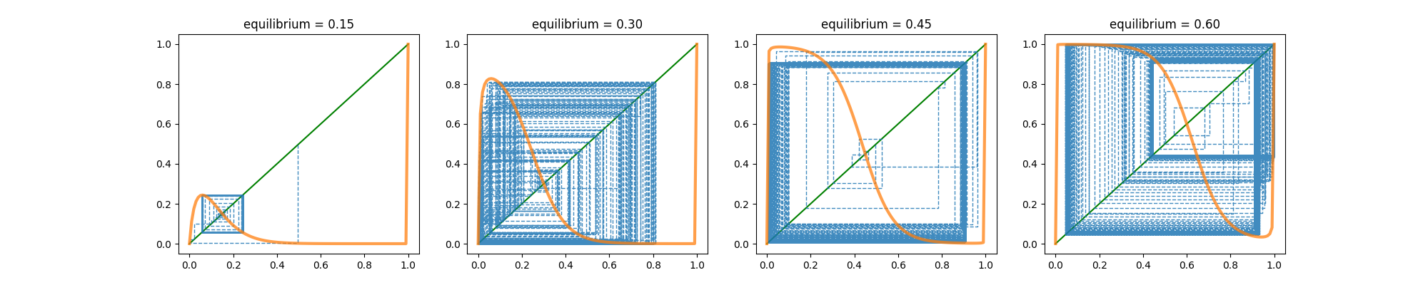
Figure 4. The cobweb diagram above displays the trajectory of iterates for the time-varying learning rate dynamics in (2), considering various equilibrium choices. The patterns formed by these paths reveal insights into the iterative behavior of the dynamics. Fixed points are identified by the intersection of the $y=x$ diagonal line and the limit function graph $\text{MWU}(x,\lim_{n\to\infty}a_{n},\text{Equilibrium})$, with spirals converging towards these points. Period-2 orbits create rectangles, while higher-period cycles generate increasingly complex closed loops. Chaotic orbits, conversely, occupy an area, indicating an infinite sequence of non-repeating values. This phenomenon intensifies as we move further from the boundaries.

∎

Appendix D Bifurcation Plots

In this section, we showcase a series of bifurcation diagrams illustrating the adaptive scheme’s limit behavior in response to varying constraints on $a_{\infty}$. These diagrams display the emergence of periodic points as a function of the proportion of users favoring the first link in the equilibrium state of the system (parameter $b$). A notable observation from these bifurcation plots is their symmetric nature. For instance, we anticipate analogous behavior when the equilibrium state accommodates 80% of users favoring the first link in the congestion game and when it accommodates 20%. This symmetry implies an inherent balance in the system’s response to changes in user preferences.

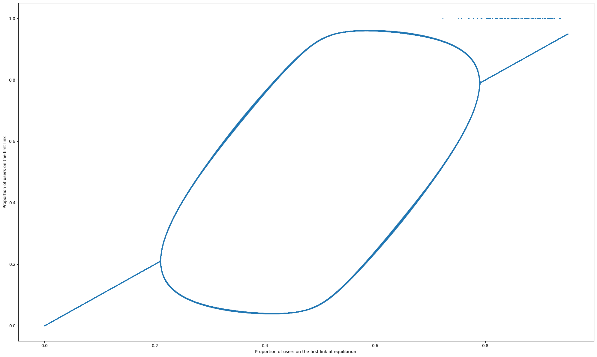
Figure 5. When the limit behavior $a_{\infty}$ is small the only system attractors are equilibria (roughly for $b<0.2$ and $b>0.8$) and period-two cycles.

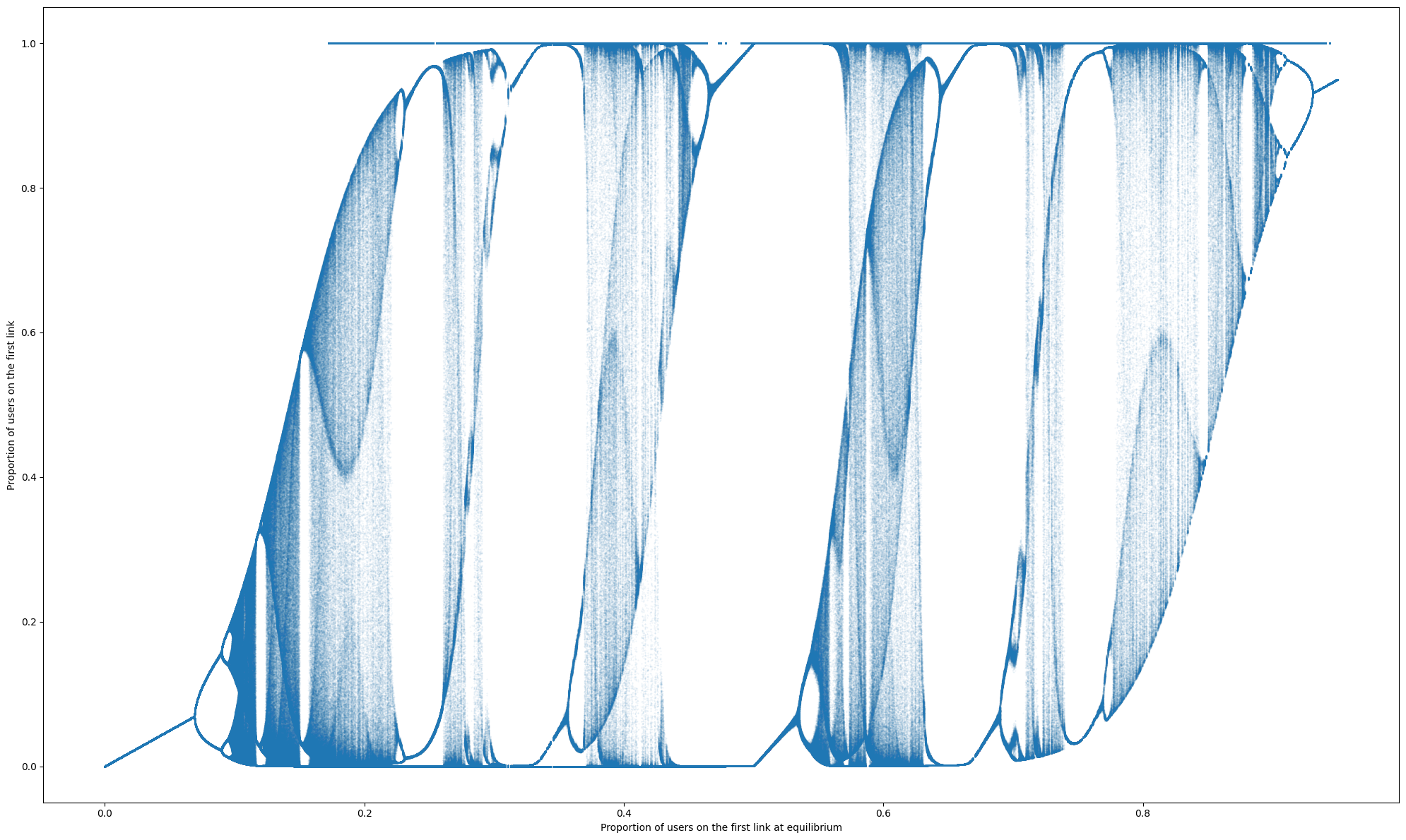
(a) When the limit behavior $a_{\infty}$ is significantly larger, which signifies a more volatile, highly fluctuating system, we see the emergence of more complex attractors, i.e., periodic orbits of large period, chaos.

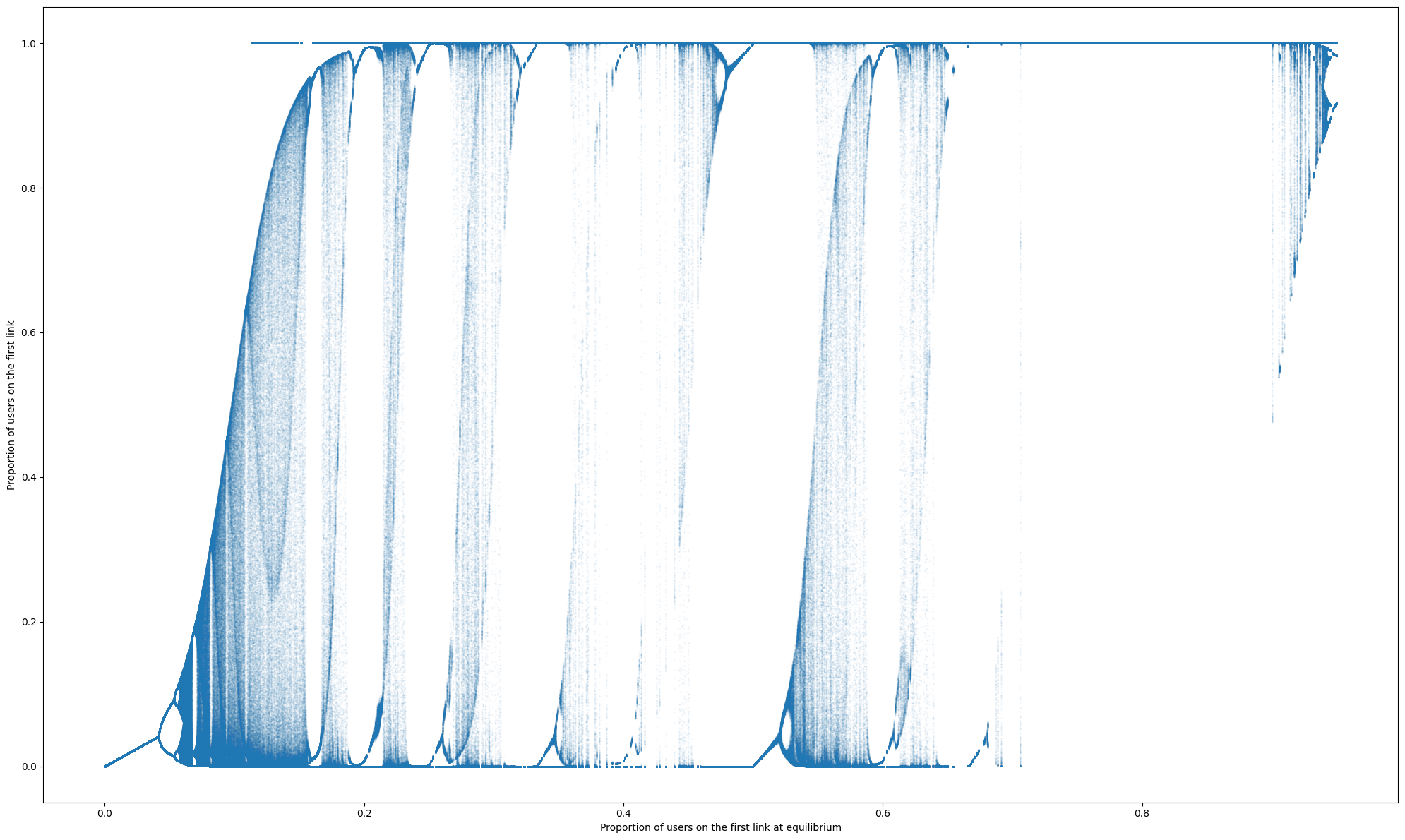
(b) Even more aggressive schemes imply the creation of complex attractors even when the equilibrium $b$ is much closer to the boundary i.e. to $0$ or $1$, in comparison with Fig. 6(a).

Figure 6. Increased Limit behavior $a_{\infty}$

References

- Abdallah & Lesser [2008] Abdallah, S. and Lesser, V. A multiagent reinforcement learning algorithm with non-linear dynamics. Journal of Artificial Intelligence Research, 33:521–549, 2008.
- Andrade et al. [2021] Andrade, G. P., Frongillo, R., and Piliouras, G. Learning in matrix games can be arbitrarily complex. In Belkin, M. and Kpotufe, S. (eds.), Proceedings of Thirty Fourth Conference on Learning Theory, volume 134 of Proceedings of Machine Learning Research, pp. 159–185. PMLR, 15–19 Aug 2021. URL https://proceedings.mlr.press/v134/andrade21a.html.
- Arora et al. [2012] Arora, S., Hazan, E., and Kale, S. The multiplicative weights update method: a meta-algorithm and applications. Theory of Computing, 8(1):121–164, 2012.
- Bailey & Piliouras [2018] Bailey, J. P. and Piliouras, G. Multiplicative weights update in zero-sum games. In Proceedings of the 2018 ACM Conference on Economics and Computation, pp. 321–338. ACM, 2018.
- Bailey & Piliouras [2019] Bailey, J. P. and Piliouras, G. Fast and furious learning in zero-sum games: Vanishing regret with non-vanishing step sizes. In Advances in Neural Information Processing Systems, volume 32, pp. 12977–12987, 2019.
- Bailey et al. [2020] Bailey, J. P., Gidel, G., and Piliouras, G. Finite regret and cycles with fixed step-size via alternating gradient descent-ascent. In Conference on Learning Theory, pp. 391–407. PMLR, 2020.
- Balduzzi et al. [2018] Balduzzi, D., Racanière, S., Martens, J., Foerster, J. N., Tuyls, K., and Graepel, T. The mechanics of n-player differentiable games. In Dy, J. G. and Krause, A. (eds.), Proceedings of the 35th International Conference on Machine Learning, ICML 2018, Stockholmsmässan, Stockholm, Sweden, July 10-15, 2018, volume 80 of Proceedings of Machine Learning Research, pp. 363–372. PMLR, 2018. URL http://proceedings.mlr.press/v80/balduzzi18a.html.
- Banerjee & Peng [2003] Banerjee, B. and Peng, J. Adaptive policy gradient in multiagent learning. In Proceedings of the second international joint conference on Autonomous agents and multiagent systems, pp. 686–692, 2003.
- Bielawski et al. [2021] Bielawski, J., Chotibut, T., Falniowski, F., Kosiorowski, G., Misiurewicz, M., and Piliouras, G. Follow-the-regularized-leader routes to chaos in routing games. In ICML, 2021.
- Bloembergen et al. [2015] Bloembergen, D., Tuyls, K., Hennes, D., and Kaisers, M. Evolutionary dynamics of multi-agent learning: A survey. Journal of Artificial Intelligence Research, 53:659–697, 2015.
- Bowling [2004] Bowling, M. Convergence and no-regret in multiagent learning. Advances in neural information processing systems, 17, 2004.
- Bowling & Veloso [2002] Bowling, M. and Veloso, M. Multiagent learning using a variable learning rate. Artificial Intelligence, 136(2):215–250, 2002.
- Cheung & Piliouras [2019] Cheung, Y. K. and Piliouras, G. Vortices instead of equilibria in minmax optimization: Chaos and butterfly effects of online learning in zero-sum games. In Conference on Learning Theory, pp. 807–834. PMLR, 2019.
- Cheung & Piliouras [2020] Cheung, Y. K. and Piliouras, G. Chaos, extremism and optimism: Volume analysis of learning in games. In Advances in Neural Information Processing Systems (NeurIPS), 2020.
- Cheung & Tao [2021] Cheung, Y. K. and Tao, Y. Chaos of learning beyond zero-sum and coordination via game decompositions. In International Conference on Learning Representations (ICLR), 2021.
- Cheung et al. [2021] Cheung, Y. K., Leonardos, S., and Piliouras, G. Learning in markets: Greed leads to chaos but following the price is right. 2021.
- Chotibut et al. [2020] Chotibut, T., Falniowski, F., Misiurewicz, M., and Piliouras, G. The route to chaos in routing games: When is price of anarchy too optimistic? In Advances in Neural Information Processing Systems (NeurIPS), 2020.
- Daskalakis et al. [2006] Daskalakis, C., Goldberg, P. W., and Papadimitriou, C. H. The complexity of computing a nash equilibrium. In Proceedings of the Thirty-Eighth Annual ACM Symposium on Theory of Computing, STOC ’06, pp. 71–78, New York, NY, USA, 2006. Association for Computing Machinery. ISBN 1595931341. doi: 10.1145/1132516.1132527. URL https://doi.org/10.1145/1132516.1132527.
- Flokas et al. [2020] Flokas, L., Vlatakis-Gkaragkounis, E.-V., Lianeas, T., Mertikopoulos, P., and Piliouras, G. No-regreet learning and mixed nash equilibria: They do not mix. In NeurIPS, 2020.
- Freund & Schapire [1999] Freund, Y. and Schapire, R. E. Adaptive game playing using multiplicative weights. Games and Economic Behavior, 29(1-2):79–103, 1999.
- Galla & Farmer [2013] Galla, T. and Farmer, J. D. Complex dynamics in learning complicated games. Proceedings of the National Academy of Sciences, 110(4):1232–1236, 2013. ISSN 0027-8424.
- Giannou et al. [2021] Giannou, A., Vlatakis-Gkaragkounis, E. V., and Mertikopoulos, P. Survival of the strictest: Stable and unstable equilibria under regularized learning with partial information. In Belkin, M. and Kpotufe, S. (eds.), Proceedings of Thirty Fourth Conference on Learning Theory, volume 134 of Proceedings of Machine Learning Research, pp. 2147–2148. PMLR, 15–19 Aug 2021. URL https://proceedings.mlr.press/v134/giannou21a.html.
- Hart & Mas-Colell [2003] Hart, S. and Mas-Colell, A. Uncoupled dynamics do not lead to nash equilibrium. American Economic Review, 93(5):1830–1836, 2003.
- Hsieh et al. [2021] Hsieh, Y.-P., Mertikopoulos, P., and Cevher, V. The limits of min-max optimization algorithms: Convergence to spurious non-critical sets. In International Conference on Machine Learning, pp. 4337–4348. PMLR, 2021.
- Kaisers et al. [2009] Kaisers, M., Tuyls, K., Parsons, S., and Thuijsman, F. An evolutionary model of multi-agent learning with a varying exploration rate. In Proceedings of The 8th International Conference on Autonomous Agents and Multiagent Systems-Volume 2, pp. 1255–1256, 2009.
- Leonardos & Piliouras [2022] Leonardos, S. and Piliouras, G. Exploration-exploitation in multi-agent learning: Catastrophe theory meets game theory. Artificial Intelligence, 304:103653, 2022.
- Leonardos et al. [2021] Leonardos, S., Monnot, B., Reijsbergen, D., Skoulakis, E., and Piliouras, G. Dynamical analysis of the eip-1559 ethereum fee market. In Proceedings of the 3rd ACM Conference on Advances in Financial Technologies, pp. 114–126, 2021.
- Letcher [2021] Letcher, A. On the impossibility of global convergence in multi-loss optimization, 2021.
- Li & Yorke [1975] Li, T.-Y. and Yorke, J. A. Period three implies chaos. The American Mathematical Monthly, 82(10):985–992, 1975.
- Littlestone & Warmuth [1994] Littlestone, N. and Warmuth, M. K. The weighted majority algorithm. Inf. Comput., 108(2):212–261, February 1994. ISSN 0890-5401. doi: 10.1006/inco.1994.1009. URL http://dx.doi.org/10.1006/inco.1994.1009.
- Mertikopoulos et al. [2018] Mertikopoulos, P., Papadimitriou, C., and Piliouras, G. Cycles in adversarial regularized learning. In Proceedings of the Twenty-Ninth Annual ACM-SIAM Symposium on Discrete Algorithms, SODA ’18, pp. 2703–2717, USA, 2018. Society for Industrial and Applied Mathematics. ISBN 9781611975031.
- Nisan et al. [2007] Nisan, N., Roughgarden, T., Tardos, E., and Vazirani, V. V. Algorithmic Game Theory. Cambridge University Press, New York, NY, USA, 2007. ISBN 0521872820.
- Palaiopanos et al. [2017] Palaiopanos, G., Panageas, I., and Piliouras, G. Multiplicative weights update with constant step-size in congestion games: Convergence, limit cycles and chaos. In Advances in Neural Information Processing Systems, pp. 5872–5882, 2017.
- Piliouras & Yu [2022] Piliouras, G. and Yu, F.-Y. Multi-agent performative prediction: From global stability and optimality to chaos. arXiv preprint arXiv:2201.10483, 2022.
- Ratcliffe et al. [2019] Ratcliffe, D. S., Hofmann, K., and Devlin, S. Win or learn fast proximal policy optimisation. In 2019 IEEE Conference on Games (CoG), pp. 1–4. IEEE, 2019.
- Roughgarden & Tardos [2002] Roughgarden, T. and Tardos, É. How bad is selfish routing? Journal of the ACM (JACM), 49(2):236–259, 2002.
- Sanders et al. [2018] Sanders, J. B. T., Farmer, J. D., and Galla, T. The prevalence of chaotic dynamics in games with many players. Scientific reports, 8(1):1–13, 2018.
- Schulman et al. [2017] Schulman, J., Wolski, F., Dhariwal, P., Radford, A., and Klimov, O. Proximal policy optimization algorithms. arXiv preprint arXiv:1707.06347, 2017.
- Shalev-Shwartz et al. [2011] Shalev-Shwartz, S. et al. Online learning and online convex optimization. Foundations and trends in Machine Learning, 4(2):107–194, 2011.
- Shi & Yu [2006] Shi, Y. and Yu, P. Study on chaos induced by turbulent maps in noncompact sets. Chaos, Solitons & Fractals, 28(5):1165–1180, 2006.
- Shub [1987] Shub, M. Global Stability of Dynamical Systems. Springer-Verlag, 1987.
- Singh et al. [2000] Singh, S., Kearns, M. J., and Mansour, Y. Nash convergence of gradient dynamics in general-sum games. In UAI, pp. 541–548. Citeseer, 2000.