ITR: Grammar-based graph compression supporting fast triple queries.

Abstract

Neighborhood queries are the most common queries on graphs; thus, it is desirable to answer them efficiently on compressed data structures. We present a compression scheme called Incidence-Type-RePair (ITR) for graphs with labeled nodes and labeled edges based on RePair [1] and apply the scheme to network, version, and RDF graphs. We show that ITR performs neighborhood queries and triple queries in only a few milliseconds and thereby outperforms existing solutions while providing a compression size comparable to existing graph compressors.

Introduction

Obtaining a node or all nodes in a graph that are adjacent to a given node is fundamental to most graph algorithms. Therefore, these neighborhood queries are the most common queries in graph processing. Whenever huge graphs, for example, network, version, or RDF graphs, are compressed, and neighborhood queries are heavily used on these compressed graphs, their performance is crucial for improving the efficiency of graph processing and the analysis of large-scale graphs. We investigate the execution time of neighborhood queries and the more general triple queries on compressed graphs generated by different graph compressors, and we introduce Incidence-Type-RePair (ITR), a grammar-based compressor that generates a compressed graph on which nearly all triple queries are answered significantly faster than on other compressed data formats for these graphs.

Like RePair [1], ITR uses context-free grammars for compression and repeatedly replaces a most frequent digram by a new nonterminal. The term digram describes two adjacent elements. For a string $ababab$, $ab$ is a digram of two adjacent letters and the grammar $\{S\rightarrow AAA,A\rightarrow ab\}$ results from replacing $ab$ by $A$ in $ababab$.

Grammar-based compression schemes have been shown to improve the efficiency of queries on compressed data, for example, for consecutive symbol visits on strings [2] and for parent/child navigations on trees [3]. RePair has been generalized to trees [4]. Furthermore, Maneth et al. [5] and Röder et al. [6] both apply RePair to graphs and define digrams to be two edges sharing a common node. As explained in Maneth et al. [5], finding a largest possible set of non-overlapping occurrences for a single digram, requires $\mathcal{O}{(|V|^{2}|E|)}$ time and is thus infeasible. Instead, they and we present different approximations on how to define and find frequent digrams.

The $k^{2}$-tree approach by Brisaboa [7, 8] is a succinct data structure for unlabeled graphs. The $k^{2}$-Triples approach by Álvarez-García et al. [9] is an adaptation of the $k^{2}$-tree approach for RDF graphs.

HDT is an RDF compressor by Fernández et al. [10] that splits a file into a header that contains information about the compressed RDF graph, the graph structure, and a dictionary. Hernández-Illera [11] improved HDT to HDT++ by using predicate families to represent all predicates of a subject by one ID.

Our ITR graph compressor uses the hyperedge replacement grammars differently from Maneth et al. [5] and Röder et al. [6], extends them to node labels, and uses $k^{2}$-trees and index-functions to optimize compression and query processing.

The main contributions of this paper are:

• ITR, an algorithm combining labeled edges and node labels to hyperedges;

• a digram definition that simplifies and speeds-up finding and replacing all occurrences of a most frequent digram;

• the index-functions, which optimize the compression of loops;

• the substitution of frequent node labels by hyperedges to reduce the number of dictionary entries;

• an evaluation comparing ITR to gRePair, RDFRePair, and different implementations of HDT [10] and $k^{2}$-tree [7] regarding compression size and runtime of neighborhood queries and triple queries that shows that ITR outperforms the other implementations of graph compressors in executing nearly all triple queries.

Preliminaries

A ranked alphabet $\Sigma$ is a set of symbols with a function $rank:\Sigma\rightarrow\mathbb{N}\backslash\{0\}$ that maps each symbol to its rank. Let $L$ be a ranked alphabet called labels. A hypergraph is a pair $G=(V_{G},E_{G})$ with nodes $V_{G}=\{0,1,\ldots,p\}\subset\mathbb{N}$ and edges $E_{G}\subset L\times V_{G}^{*}$. We write $e=a(v_{0},\ldots,v_{n-1})$ for an edge $e\in E_{G}$ with $label(e)=a$ and $rank(e)=n$. The rank describes the number of nodes (including duplicates) that are connected to the edge. We call all elements in $E_{G}$ edges regardless of their rank, and we use the term hyperedge to emphasize that a concept needs non-rank-2 edges. Let $\mathbb{G}$ be the set of all hypergraphs.

We write $e[m]=v_{m}$ for the node $v_{m}$ that is connected to $e=a(v_{0},\ldots,v_{n-1})\in E_{G}$, and we call $m$ the connection-type of $v_{m}$ to the edge $e$. We always assume $m$ to be well defined, that is $0\leq m<n=rank(e)$. For example, an edge $e=f(10,11)\in E_{G}$ has $label(e)=f$, $rank(e)=2$, and connection-type $0$ for node $e[0]=10$. For each edge of rank 2, there are two connection-types, where 0 is equivalent to ‘outgoing’ from the source node and 1 is equivalent to ‘incoming’ to the destination node. We assume that for all symbols $a\in L$ and for all edges $e\in E$ with $label(e)=a$, $rank(e)$ is unique and equal to $rank(a)$, that is, all edges with the same label have the same rank.

Similar to Maneth et al. [5], we define a Hyperedge replacement grammar (HR grammar) as a tuple $H=(T,N,P,S)$ with $T$ and $N$ being ranked alphabets with $N\cap T=\emptyset$, $T\cup N=L$, $P\subset N\times\mathbb{G}$, and $S\in N$. We call an edge $e$ terminal if $label(e)\in T$, and we call $e$ nonterminal if $label(e)\in N$. We write $A\rightarrow G_{A}$ for a rule $(A,G_{A})\in P$. The right-hand side $G_{S}$ of the grammar rule $S\rightarrow G_{S}$ is called start graph.

We construct only straight-line HR grammars (SL-HR grammars). For straight-line grammars, the following conditions hold: (1) for each nonterminal in $N$ exists exactly one rule in $P$ and (2) the grammar is non-recursive. These grammars produce only one word, which is the uncompressed graph. We denote the uncompressed graph of the SL-HR grammar $H$ by $\psi(H)\in\mathbb{G}$.

However, ITR differs from the approaches of Maneth et al. [5] and Röder et al. [6] by our succinct encoding of the edges that replaces loops implicitly. A loop means that an edge has more than one connection to the same node. In Figure 1 (a) and (b) there are loops, both at node $10$. Because loops are replaced in our succinct encoding, our digram definition does not need to distinguish whether or not edges have loops.

To define digrams, we first define the incidence-type $i$ as the pair $(a,m)$ of an edge label $a\in L$ and a connection-type $m\in\mathbb{N}$ with $m<rank(a)$. We define the set of all incidence-types $IT=\{(a,m)\in L\times\mathbb{N}\text{ | }0\leq m<rank(a)\}$.

Figure 1: Example replacement of digram $d=((g,~{}1),(f,~{}0))$ from subfigure (a) to (b) introducing the rule $B$ shown in (d), and replacement of the loop of the edge $B(10,10,11)$ from (b) to (c) introducing the rule $C$ shown in (e). In the digram $d$, $(g,~{}1)$ means an incoming edge with label $g$ and $(f,~{}0)$ means an outgoing edge with label $f$.

A digram $d$ is a pair of two possibly equal incidence-types $(a_{1},m_{1}),(a_{2},m_{2})\in IT$. An occurrence of a digram $d=((a_{1},m_{1}),(a_{2},m_{2}))$ is a pair of two edges $(e_{1},e_{2})$ with $e_{1}\neq e_{2}$, $label(e_{1})=a_{1}$, $label(e_{2})=a_{2}$, and $e_{1}[m_{1}]=e_{2}[m_{2}]$. So, the two edges $(e_{1},e_{2})$ are different, fit to the labels of $d$, and share a common node. Let $\mathbb{D}$ be the set of all digrams.

For example, in Figure 1 (a), for the digram $d=((g,1),(f,0))$, we find the occurrences $o_{1}=(g(11,12),f(12,13))$ and $o_{2}=(g(10,10),f(10,11))$. Compression replaces the edges of the occurrences $o_{1}$ and $o_{2}$ by $B(12,11,13)$ and $B(10,10,11)$, as shown in Figure 1 (b). In addition, the rule $B\rightarrow(\{0,1,2\},\{g(1,0),f(0,2)\})$, which is visualized in Figure 1 (d), is added to the grammar. We do not replace $o_{3}=(g(10,10),f(10,12))$, because $o_{3}$ shares an edge with $o_{2}$, thereby we cannot replace both, $o_{2}$ and $o_{3}$.

The reverse step of replacing a digram occurrence is expanding and replacing. Expanding the edge $B(12,11,13)$ applies the rule $B\rightarrow(\{0,1,2\},\{g(1,0)\,f(0,2)\})$ with its formal node parameters $0,1,2$ to the actual nodes $12,11,13$ which generates the set $\{g(11,12),f(12,13)\}$ of edges. By expanding both edges with label $B$ in the graph of Figure 1 (b) and replacing them with the generated sets of edges, we get the decompressed graph of Figure 1 (a).

An implication of our definition of digrams is that we only have 3 shapes of digrams for two edges of rank 2 in contrast to 33 or more shapes of Röder et al. [6]. Our three shapes have a given common node and either two outgoing edges, two incoming edges, or one incoming and one outgoing edge. In comparison to Röder et al. [6], we save less space by replacing a single occurrence, but we replace more occurrences of a single digram.

Compression

We separate the graph structure from the text and establish the connection between both parts by IDs, which is common practice [5, 6, 8, 10, 11].

The RePair algorithm consists of two steps: Replace Digrams (shown in Algorithm 1) and Prune. We omit presenting the Prune step because it is a straight-forward adaptation of the Prune step from String RePair [1]. We discuss the steps Count (Line 1), Update Count (Line 6), and Replace (Line 5).

Input: grammar

1 Count occurrences of digrams

2 $mfd\textbf{ }{}\leftarrow{}\textbf{ }{}\text{most frequent digram}$

3 while replacing the mfd reduces grammar size do

4       $\text{Define a new rule for $mfd$ with a new nonterminal }A_{mfd}$

5       $\text{Replace each occurrence of $mfd$ with an edge with label }A_{mfd}$

6       Update digram count

7       $mfd\textbf{ }{}\leftarrow{}\textbf{ }{}\text{select next most frequent digram}$

8      

Algorithm 1 $replaceDigrams$

Line 1, Count: To get the maximum number of non-overlapping occurrences of a digram, Maneth et al. [5] mention an algorithm with runtime $\mathcal{O}(|V|^{2}|E|)$. Instead, we approximate the count of digrams in two steps. Our digrams consists of two incidence-types, so we first count the frequency of incidence-types at each node by a single scan over all edges. The result is a mapping $c:V\times IT\rightarrow\mathbb{N}$. For example, in Figure 1 (a), the node $10$ has two outgoing edges with label $f$, so $c(10,(f,0))=2$. To define $count:\mathbb{D}\rightarrow\mathbb{N}$, we use $c$ in the following way: For every node $v$ and for every two incidence-types $i_{1}$ and $i_{2}$ occurring at the node $v$, we determine the number of occurrences $count_{v}(i_{1},i_{2})$ of the digram $(i_{1},i_{2})$ at the node $v$ by

$$count_{v}(i_{1},i_{2}):=\begin{cases}\min(c(v,i_{1}),c(v,i_{2}))&\text{ if }i_{1}\neq i_{2}\\ \left\lfloor\frac{c(v,i_{1})}{2}\right\rfloor&\text{ if }i_{1}=i_{2}.\end{cases}$$

In Figure 1 (a), we have for example $c(10,(f,0))=2$ and $c(10,(g,0))=1$. From these two values of $c$, we obtain that at node $10$, there is one occurrence of each of the digrams ($(f,0)$,$(f,0)$) and ($(f,0)$,$(g,0)$) and there is no occurrence of the digram $((g,0),(g,0))$. We define $count:\mathbb{D}\rightarrow\mathbb{N}$ by

$$count((i_{1},i_{2}))=\sum_{v\in V}count_{v}(i_{1},i_{2})$$

Line 6, Update Count: We store both, $c$ and $count$, from the step Count of Line 1. When we replace an edge $e$ with $label(e)=a$, we consider all nodes $v$ of $e$ and all incidence-types $i_{1}=(a,m)$ such that $e[m]=v$ and reduce $c(v,i_{1})$ by 1 accordingly. Then, we reduce the number $count((i_{1},i_{2}))$ of all digram occurrences of digrams $d=(i_{1},i_{2})$ for all incidence-types $i_{2}$ with $c(v,i_{2})>0$ by 1 if and only if

$$i_{1}\neq i_{2}\text{ and }c(v,i_{1})\leq c(v,i_{2})\text{ or }i_{1}=i_{2}\text{ and }c(v,i_{1})\text{ is even}.$$

This adjustment has the same result as if we would count the number of digrams calling Line 1 of Algorithm 1 again. The steps to increase the counts for the new nonterminal edge are analogous.

Line 5, Replace: We find occurrences of a digram $d=((a_{1},m_{1}),(a_{2},m_{2}))$ by a left-to-right scan of the edge list and by saving pointers to edges that have one of the labels of $d$. Let $e_{1}$ have $label(e_{1})=a_{1}$. Then, we store a pointer to $e_{1}$ according to the node $e_{1}[m_{1}]$. If we already had a pointer to $e_{2}$ with $label(e_{2})=a_{2}$, $e_{2}[m_{2}]=e_{1}[m_{1}]$, and $e_{1}\neq e_{2}$, $(e_{1},e_{2})$ is an occurrence of $d$. In this case, we delete the pointers to $e_{1}$ and $e_{2}$ and replace $e_{1}$ and $e_{2}$ with a new hyperedge having label $A_{d}$. We want $e_{1}\neq e_{2}$ to avoid replacing a loop as an occurrence. In Figure 1 (a), we replace two occurrences of the digram $((g,1),(f,0))$, that occur at node $10$ and at node $12$ with one edge with label $B$ each, yielding the graph of Figure 1 (b).

Succinct Encoding.

Our encoding of the start graph $G_{S}$ is based on $k^{2}$-trees [7] of the incidence-matrix $M$ of $G_{S}$ and is shown in Figure 2. First, we sort the edges by the ID of their label and encode the monotonically increasing list of the IDs by the Elias-Fano-encoding [12]. The incidence-matrix $M$ has a $1$ in row $i$ and column $j$ if and only if edge $j$ is connected to node $i$. For example, in Figure 2 (b), $e_{2}=B(10,10,11)$ is an edge. $M$ contains a 1 at the positions $(10,2)$ and $(11,2)$, but it does not contain the information how often and at which connection-types the node $10$ occurs in edge $e_{2}$. We introduce the index-function to close this information gap.

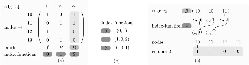
Figure 2: (a) illustrates the implementation of the succinct encoding. One edge in the start rule is represented by three parts: a column of the incidence matrix, a label and an ID of an index-function. (b) shows the IDs and the corresponding index-functions, and (c) shows how the index-function 2 stores the order and the repetitions of nodes $\zeta_{e_{2}}=[10,11]$ of edge $e_{2}$.

Let $\zeta_{e}$ be the duplicate-free and sorted list of nodes of $e$. In the example, $\zeta_{e_{2}}$ is $[10,11]$. Let $k$ be the length of $\zeta_{e}$. The index-function $\pi_{e}:\{0,\ldots,{rank(e)-1}\}\rightarrow\{0,\ldots k-1\}$ maps each connection-type $m$ of the edge $e$ to its index in the list $\zeta_{e}$. Formally, $e[m]=\zeta_{e}[\pi_{e}(m)]$. We write the index-function as ${(\pi_{e}(0),\ldots,\pi_{e}(rank(e)-1))}$. In the example of Figure 2 (b), $\pi_{e_{2}}=(0,0,1)$. Thereby, each edge is uniquely reconstructable by its column in $M$ together with its index-function and its label. Instead of saving the same index-function multiple times, we assign IDs to all index-functions. We use the $\delta$-code [13] to encode $\pi$ as $\delta(rank(e)-1)$$\delta(\pi(0))\ldots\delta(\pi(rank(e)-1))$.

Like Maneth et al. [5], we encode all graphs of rules except the start graph by only encoding the right-hand sides of the rules because the order of rules determines their nonterminal. For each right-hand side, we first encode the number of edges and then, for each edge, the label and its nodes. For example, the sequence of edges $d(0,1)$ and $B{}(1,2,0)$ is encoded by $\delta{}(2)$ $\delta{}(d)\delta{}(0)\delta{}(1)$ $\delta{}(B)\delta{}(1)\delta{}(2)\delta{}(0)$.

Handling loops in the grammar.

In Figure 1 (b), we have an edge $e=B(10,10,11)$ that is connected twice to node $10$ and thereby is a loop. We could introduce an extra rule $C{}\rightarrow{}(\{0,1\},\{B(0,0,1)\})$ as in Figure 1 (e) and replace the edge $e$ by $C(10,11)$ yielding the graph of Figure 1 (c). This is a tradeoff: We introduce more rules, but we reduce the number of nodes that are used as a parameter in rules by 1 for each occurrence of such a loop. An evaluation of the implementation shows that these extra rules do not improve compression, because the index-function that is used in the succinct encoding also removes the duplicate parameters. Therefore, we do not replace loops by introducing extra rules, and also because skipping this step reduces the time needed to compress a graph.

Answering triple queries.

Simple graph queries written as triples are more general than neighborhood queries. Each component of a triple query is bound (as in S P O for RDF graphs) or unbound (as in ?S ?P ?O).

Given an SL-HR grammar $H$ with start rule $S\rightarrow{}G_{S}$, we answer a triple query based on its bound parameters. We use a set $Z$ to store intermediate results.

• Case 1, S or O are bound: Let $r$ be the value of S, or of O if S is unbound. To compute set $Z$, we first decompress the row $r$ of the incidence-matrix $M$ of $G_{S}$. This is done without decompressing the whole incidence-matrix [7]. Each column $j$ with a 1 in row $r$ represents an edge $e_{j}$ that is connected to node $r$, and we add the edge $e_{j}$ to $Z$.

• Case 2, only P is bound: An edge with label P can be in the start graph or be generated by a nonterminal edge $e$ with label $A$. We lookup in a matrix $NT$, whether or not $e$ creates edges with label P. The matrix $NT$ contains a row for each nonterminal label $A_{y}$ in the grammar and a column for each terminal label $a_{x}$, and there is a 1 in $NT$ if and only if $A_{y}$ generates at least one edge with $a_{x}$ as label. $NT$ is compressed by $k^{2}$-trees. If $e$ generates edges with label P, we add $e$ to $Z$. We use the binary search on the sorted list of edge labels.

• Case 3, the query is ?S ?P ?O: The query is equivalent to the decompression. We add all edges of the start rule to $Z$.

In all three cases, while there is an edge $e\in{}Z$:

• If $e$ is a nonterminal and

  • (S is unbound or $e$ is connected to S for any connection-type) and

  • (O is unbound or $e$ is connected to O for any connection-type) and

  • (P is unbound or $NT$ has the value $1$ at row $label(e)$ and column P),

  • expand $e$ and extend $Z$ by the set of edges generated by expanding $e$.

• If $e$ is a terminal and $e$ is a solution to the query,

  • output $e$.

In all cases, remove $e$ from $Z$, and proceed with a new $e\in{}Z$.

ITR+: Improved compression of frequent node labels

ITR+ is an extension of ITR, that increases the compression further. For example, the ttt-win graph of the game tic-tac-toe contains only 3 node labels, x and o for the players, and b for a blank field. Like gRePair [5] and RDFRePair [6], ITR stores $|V|=5634$ RDF representations of these three labels in the dictionary, because the RDF representations are slightly different for all $5634$ nodes. However, ITR+ includes the labels x, o and b as edges of rank 1 into the graph; for example, x(1) means that the node with ID 1 has the label x. Thereby, ITR+ stores only three labels for these edges in the dictionary instead of $5634$ labels for nodes. Furthermore, edges of rank 1 can be part of a digram replacement with other edges. Thereby, ITR+ compresses frequent subgraphs of node labels and edge labels into single nonterminals. Thus, ITR+ reduces the compression ratio of the ttt-win graph to 14.23% of the uncompressed graph, which outperforms all other approaches. On the other hand, ITR+ increases the number of edges from $|E|$ to $|E|+|V|$ and for this optimization, the graph must contain the same node label for multiple nodes.

The gRePair implementation is not capable of using edges of rank 1 as terminals and RDFRePair is designed only for edges of rank 2. Therefore, the ability to treat frequent node labels as hyperedges of rank 1 and thereby compress the graph stronger is unique to ITR+.

Experimental results

Name	Language	Query Type
ITR	C	triple
RDFRePair	Java	-
gRePair	Scala	Neighborhood
HDT-java	Java	SPARQL
HDT++	C++	triple
$k^{2}$-java	Java	SPARQL
$k^{2}$++	C++	-

(a)

File	$|V|$	$|E|$	$|T|$
homepages-en	98665	50000	1
geo-coordinates-en	46107	50000	4
jamendo	396531	1047951	25
wikidata	10051660	42922799	635
archiveshub	280556	1361816	139
scholarydata-dump	140042	1159985	84
chess-legal	76272	113039	12
ttt-win	5634	10016	3
WikiTalk	2394385	5021410	1
NotreDame	325729	1497134	1
CA-AstroPh	18772	396160	1

(b)

Table 1: (a) Compared implementations of the compression algorithms. (b) Datasets used for testing, sorted by the edge per node ratio $\frac{|E|}{|V|}$. The number of labels of a dataset is listed in column $|T|$.

We investigate the time needed to answer a neighborhood query or a triple query. We compare results of the compressors listed in Table 1 (a). We test all implementations on a Debian 5.10.149-2 machine with 128GB RAM and 2 Cores @ 2.30GHz. For the tests, we use the RDF graphs homepages-en, geo-coorindates-en, jamendo, wikidata, archiveshub, scholarydata-dump as in Röder et al. [6], the version graphs ttt-win and chess-legal from SUBDUE and the webgraphs CA-AstroPh, NotreDame and WikiTalk from the Standford Large Network Dataset Collection [14]. As not all compressors are designed to use webgraphs and version-graphs as input, we converted their structure to an RDF notation and take these converted files as input for all approaches for fairness.

ITR is implemented in C. For the $k^{2}$-tree approach, we use the implementations of Röder et al. [6] as in their paper in Java and C++, $k^{2}$-java and $k^{2}$++, respectively. We include two implementations of HDT, HDT-java and HDT++.

In Figure 3, we see that ITR compresses stronger than the existing solutions on some datasets like geo-coordinates, and archiveshub, but other approaches compress stronger on the network and version graphs due to a non-optimal dictionary compression.

For the runtime comparison summarized in Figure 4, we include all times needed for IO-operations as not all compressors output their time for performing the query without IO-operations. We exclude the build time and disk space used by HDT-java and HDT++ for additional indices.

Due to the different supported query types, we compare the runtime by using queries that are equal if possible. For example, we use SELECT ?pr ?ob WHERE { v ?pr ?ob } as SPARQL query and v ?P ?O as triple query for an outgoing neighborhood query of the node $v$. As the gRePair implementation does not support queries with labels, gRePair is only included in the comparisons of S ? ? and ? ? O. We perform 500 queries of each query type on each file and show the average time needed to answer the queries.

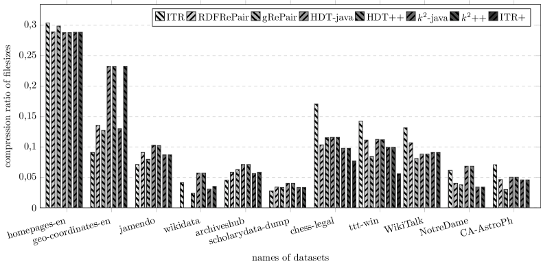
Figure 3: The compression ratio is the file size of the compressed graph divided by the file size of the uncompressed input file. We stopped RDFRePair on wikidata after 6 days.

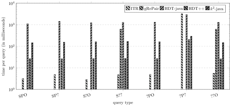
Figure 4: Average runtime in milliseconds of 500 queries each on the geo-coordinates-en graph. Implementations that do not appear in the legend do not support any type of query. gRePair can only answer neighborhood queries (S ? ? and ? ? O).

In Figure 4, we see that gRePair, HDT-java, and $k^{2}$-java as Java or Scala implementations are outperformed by the C and C++ implementations. ITR is about 2 to 6 times faster than HDT++ except for ? P ? queries. Furthermore, ITR is more than 100 times faster than gRePair.

Summary and Conclusion

We presented the ITR graph compressor based on a new type of digrams and index-functions. Futhermore, ITR+ can use hyperedges of rank 1 for frequent node labels to reduce the needed dictionary size to store node labels. Our evaluation of the runtime of triple queries shows that ITR performs all queries except ? P ? significantly faster than the existing variants of RePair on graphs, namely gRePair and RDFRePair, and faster than $k^{2}$-tree and HDT provided on different implementations.

Acknowledgements

We would like to thank Fabian Röthlinger for his support in implementing ITR.

References

References

- [1] N. J. Larsson and A. Moffat, “Off-line dictionary-based compression,” Proceedings of the IEEE, vol. 88, no. 11, pp. 1722–1732, 2000.
- [2] L. Gasieniec, R. M. Kolpakov, I. Potapov, and P. Sant, “Real-Time Traversal in Grammar-Based Compressed Files.,” in DCC. Citeseer, 2005, p. 458.
- [3] M. Lohrey, S. Maneth, and C. P. Reh, “Traversing Grammar-Compressed Trees with Constant Delay,” in 2016 Data Compression Conference (DCC), 2016, pp. 546–555.
- [4] M. Lohrey, S. Maneth, and R. Mennicke, “Tree Structure Compression with RePair,” in 2011 Data Compression Conference, 2011, pp. 353–362.
- [5] S. Maneth and F. Peternek, “Compressing graphs by grammars,” in 2016 IEEE 32nd International Conference on Data Engineering (ICDE). IEEE, 2016, pp. 109–120.
- [6] M. Röder, P. Frerk, F. Conrads, and A.-C. N. Ngomo, “Applying Grammar-Based Compression to RDF,” in The Semantic Web, Cham, 2021, pp. 93–108, Springer International Publishing.
- [7] N. R. Brisaboa, S. Ladra, and G. Navarro, “k2-Trees for Compact Web Graph Representation,” in String Processing and Information Retrieval, Berlin, Heidelberg, 2009, Springer Berlin Heidelberg.
- [8] N. R. Brisaboa, S. Ladra, and G. Navarro, “Compact representation of Web graphs with extended functionality,” Information Systems, vol. 39, pp. 152–174, 2014.
- [9] S. Álvarez-García, N. R. Brisaboa, J. D. Fernández, and M. A. Martínez-Prieto, “Compressed k2-Triples for Full-In-Memory RDF Engines,” AMCIS 2011 Proceedings - All Submissions, vol. 350., 2011.
- [10] J. Fernández, M. A. Martínez-Prieto, C. Gutierrez, A. Polleres, and M. Arias, “Binary RDF Representation for Publication and Exchange (HDT),” Journal of Web Semantics, vol. 19, pp. 22–41, 03 2013.
- [11] A. Hernández-Illera, M. A. Martínez-Prieto, and J. D. Fernández, “Serializing RDF in Compressed Space,” in 2015 Data Compression Conference, 2015, pp. 363–372.
- [12] S. Vigna, “Quasi-Succinct Indices,” in Proceedings of the Sixth ACM International Conference on Web Search and Data Mining, New York, NY, USA, 2013, WSDM ’13, p. 83–92, Association for Computing Machinery.
- [13] P. Elias, “Universal codeword sets and representations of the integers,” IEEE Transactions on Information Theory, vol. 21, no. 2, pp. 194–203, 1975.
- [14] J. Leskovec and A. Krevl, “SNAP Datasets: Stanford large network dataset collection,” http://snap.stanford.edu/data, June 2014.