Graph-Level Embedding for Time-Evolving Graphs

Abstract.

Graph representation learning (also known as network embedding) has been extensively researched with varying levels of granularity, ranging from nodes to graphs. While most prior work in this area focuses on node-level representation, limited research has been conducted on graph-level embedding, particularly for dynamic or temporal networks. However, learning low-dimensional graph-level representations for dynamic networks is critical for various downstream graph retrieval tasks such as temporal graph similarity ranking, temporal graph isomorphism, and anomaly detection. In this paper, we present a novel method for temporal graph-level embedding that addresses this gap. Our approach involves constructing a multilayer graph and using a modified random walk with temporal backtracking to generate temporal contexts for the graph’s nodes. We then train a “document-level” language model on these contexts to generate graph-level embeddings. We evaluate our proposed model on five publicly available datasets for the task of temporal graph similarity ranking, and our model outperforms baseline methods. Our experimental results demonstrate the effectiveness of our method in generating graph-level embeddings for dynamic networks.

1. Introduction

Graphs, or networks, are prevalent in diverse domains such as social networks, protein interactions, and scientific collaboration. Graph representation learning, also known as graph embedding, enables the representation of graphs using general-purpose vector representations, removing the need for task-specific feature engineering.

Graphs can be static, where their structure does not change over time, or dynamic, where their structure evolves over time. Social networks are typically dynamic due to their constantly changing structure. Representation learning on static and dynamic networks differs as static embeddings only need to capture network structure while dynamic embeddings must capture both structural and temporal aspects. While static embedding methods can be applied to dynamic networks, the resulting embeddings do not capture the evolving aspect of these networks. Network embedding methods are categorized by granularity, from node to graph level. Node embedding is the most common method in which nodes in a given network are represented as fixed-length vectors. While these vectors preserve different scales of proximity between the nodes, such as microscopic (Perozzi et al., 2014; Grover and Leskovec, 2016; Wang et al., 2021a) and structural role (Ribeiro et al., 2017; Donnat et al., 2018; Wang et al., 2020, 2021e), they cannot capture proximity between different networks as node representations are learned within the context of the network they occupy. Notably, considerable work has been done on node embedding for dynamic graphs (Goyal et al., 2018; Li et al., 2018; Wang et al., 2021d, b), which preserves not only the network structural information but also the temporal information for each node.

Graph-level network embedding, unlike node embedding, allows us to learn representations of entire graphs and directly compare different graphs, enabling investigation of fundamental graph ranking and retrieval problems such as the degree of similarity between graphs. Graph-level embedding methods have been studied extensively in the literature, but most of them focus on static networks (Narayanan et al., 2017; Chen and Koga, 2019; Tsitsulin et al., 2018; Wang et al., 2021c). However, in real-world applications, dynamic networks are ubiquitous. To the best of our knowledge, only one prior method, called tdGraphEmbed (Beladev et al., 2020), has been proposed for dynamic graph-level embedding. However, this method has a major limitation in that it treats dynamic graphs as a collection of independent static graph snapshots, ignoring the interactions between them.

To address this gap, we propose a novel method called the temporal backtracking random walk, which, when combined with the doc2vec algorithm, can be used for dynamic graph-level embedding. Our method smoothly incorporates both graph structural and temporal information. We evaluate our method on five publicly available datasets for the task of temporal graph similarity ranking and demonstrate that it achieves state-of-the-art performance.

2. Related Work

In the introduction, we discussed tdGraphEmbed as the only existing method for dynamic graph-level embedding. In this section, we review two adjacent categories of graph embedding techniques: temporal node and static graph-level embedding.

Temporal node embedding methods differ from static node embedding methods such as node2vec (Grover and Leskovec, 2016), SDNE (Wang et al., 2016), and GAE (Kipf and Welling, 2016) in that they incorporate historical information to preserve both structural and temporal information. Matrix factorization techniques such as TMNF (Yu et al., 2017), modified random walk algorithms such as CTDNE (Nguyen et al., 2018), and deep-learning-based methods such as DynGEM (Goyal et al., 2018), dyngraph2vec (Goyal et al., 2020), and variations like DynAE, DynRNN, and DynAERNN are examples of such techniques. Additionally, DynamicTriad (Zhou et al., 2018) employs the triadic closure process to develop closed triads from open triads.

For static graph-level embedding, various methods have been proposed, including the use of graph kernels (e.g., graph2vec (Narayanan et al., 2017) employs graph kernels to extract features which are passed to a language model for embedding), random walks (Sub2Vec (Adhikari et al., 2018)), multi-scale attention (UGraphEmb (Bai et al., 2019)), and the Laplacian matrix and eigenvalues (e.g., NetLSD (Tsitsulin et al., 2018)).

3. Approach

In this section, we introduce our framework for the problem of representing each snapshot of a temporal graph as a low-dimensional vector that captures both the dynamic evolution information and graph topology.

3.1. Problem Definition

Given a discrete temporal graph $G=(V,E,T)$, where each temporal edge $(u,v){t}\in E$ is directed from node $u$ to node $v$ at time $t\in T$, a snapshot of $G$ at time $t$ is defined as $G{t}=\left(V_{t},E_{t}\right)$, which is the graph of all edges occurring at time $t$. The problem is to represent each snapshot $G_{t}$ as a low-dimensional vector $X_{t}\in\mathbb{R}^{n}$, where $n<<|V|$, that captures both the dynamic evolution information and graph topology. We solve this problem in an unsupervised way and do not require any task-specific information.

3.2. Our Framework

Our framework consists of two parts: (1) building a multilayer graph and adopting temporal backtracking random walk on it (2) learning a doc2vec language model on the output of the modified random walk to obtain graph-level embeddings. First, we construct a multilayer weighted graph $M(V_{M},E_{M})$ that encodes the evolution between nodes. Each layer $M_{t},t=0,1,\ldots,|T|$, is constructed by the nodes of $G$ and the edges of snapshot $G_{t}$. We build inter-layer edges between each pair of $M_{t}$ and $M_{t-1}$ by directly connecting the corresponding nodes from $t$ to $t-1$. Note that the edges between the two layers are unidirectional. Next, we model each snapshot $G_{t}$ by using temporal backtracking random walk from each node as a sentence. Then all the sentences are concatenated to create a document representing the entire snapshot. During each step of the temporal backtracking walk, the walker can either stay in the current layer to obtain structural information or move to the previous layer to obtain historical evolving information. We define the stay constant $\alpha$ such that the probability of staying in the current layer is $\alpha$, and the probability of going to the previous layer is $1-\alpha$. A temporal backtracking walk on $M$ is a sequence of vertices $\left\langle v_{1},v_{2},\cdots,v_{k}\right\rangle$ such that $\left\langle v_{i},v_{i+1}\right\rangle\in E_{M}$ for $1\leq i<k$, which can be derived by the transition probability on $M$. Assuming that we have got $\left\langle v_{1},v_{2},\cdots,v_{i}\right\rangle$, and $v_{i}\in M_{t}$, the transition probability at step $i+1$ is defined as:

(1) $$P\left(v_{i+1}|v_{i-1},v_{i}\right)=\begin{cases}1-\alpha&v_{i+1}\in M_{t-1}\\ \frac{\alpha}{pZ}&d_{v_{i-1},v_{i+1}}=0,v_{i+1}\in M_{t}\\ \frac{\alpha}{Z}&d_{v_{i-1},v_{i+1}}=1,v_{i+1}\in M_{t}\\ \frac{\alpha}{qZ}&d_{v_{i-1},v_{i+1}}=2,v_{i+1}\in M_{t}\\ 0&otherwise\end{cases}$$

We draw inspiration from node2vec and introduce a modified version of the algorithm to capture temporal information. In this context, $d_{u,v}$ represents the length of the shortest path between node $u$ and $v$, while $p$ and $q$ are the return and in-out parameters, respectively. These parameters smoothly interpolate breadth-first and depth-first sampling. The normalizing constant $Z$ is also used. Alias sampling is used to perform each step of the temporal backtracking random walk in $O(1)$ time complexity.

The temporal backtracking random walk combines the proximity information of nodes within a layer with the structural information of previous timestamps. This approach is facilitated by the stay constant, which is set to be larger than 0.5. This ensures that the influence of older timestamps decays smoothly as the probability of entering previous layers decreases exponentially.

We represent the context of each node in a $G_{t}$ snapshot as a sentence. These sentences are concatenated to create a document that represents the snapshot. As these sentences have no inherent order, we adopt a modified doc2vec language model to learn a representation of the snapshot “documents”. In this approach, each sentence is tagged with the corresponding timestamp ($t$ of $G_{t}$) as the paragraph id of doc2vec. The final paragraph vector obtained after training is the dynamic graph-level embedding of $G_{t}$.

	Reddit - Game of Thrones				Reddit- Formula1
	p@10	p@20	$\tau$	$\rho$	p@10	p@20	$\tau$	$\rho$
Static graph-level embedding
graph2vec	$0.260$	$0.381$	$0.038$	$0.056$	$0.169$	$0.320$	$0.043$	$0.063$
UGraphEmb	$0.278$	$0.416$	$0.046$	$0.068$	$0.238$	$0.37$	$0.026$	$0.039$
Sub2Vec	$0.160$	$0.355$	$0.022$	$0.039$	$0.182$	$0.300$	-$0.030$	-$0.040$
Temporal node-level embedding
node2vec aligned	$0.336$	$0.431$	$0.069$	$0.103$	$0.214$	$0.361$	$0.047$	$0.083$
SDNE aligned	$0.352$	$0.457$	$0.120$	$0.197$	$0.262$	$0.388$	$0.044$	$0.078$
GAE aligned	$0.235$	$0.342$	$0.044$	$0.066$	$0.200$	$0.342$	$0.036$	$0.062$
DynGEM	$0.340$	$0.441$	$0.075$	$0.113$	$0.192$	$0.339$	$0.029$	$0.045$
DynamicTriad	$0.277$	$0.364$	$0.131$	$0.195$	$0.243$	$0.396$	$0.024$	$0.033$
DynAE	$0.192$	$0.357$	$0.019$	$0.030$	$0.229$	$0.397$	$0.009$	$0.012$
DynAERNN	$0.192$	$0.349$	-$0.002$	-$0.004$	$0.164$	$0.357$	$0.026$	$0.037$
Temporal graph-level embedding
tdGraphEmbed	$0.355$	$0.457$	$0.160$	$0.232$	$\mathbf{0.274}$	$0.400$	$0.060$	$0.092$
Our method	$\mathbf{0.435}$	$\mathbf{0.481}$	$\mathbf{0.177}$	$\mathbf{0.272}$	$0.265$	$\mathbf{0.410}$	$\mathbf{0.076}$	$\mathbf{0.106}$

Table 1. The temporal similarity results. The precision at K (p@K) metric is used to evaluate the method’s accuracy. Additionally, we report Spearman’s ($\rho$) and Kendall’s ($\tau$) rank correlation coefficients to measure the method’s consistency in ranking similar pairs of snapshots across different evaluation scenarios.

4. Experiments

We evaluate the effectiveness of our dynamic graph-level embeddings by measuring their performance on the task of temporal graph similarity ranking. To this end, we use five publicly available datasets (Table 2) introduced by Beladev et al. (Beladev et al., 2020) and apply the same settings and metrics as used by them. Furthermore, we conduct scalability experiments to showcase our model’s robustness and applicability to large networks commonly found in real-world applications.

Dataset	Nodes	Edges
Reddit (Game of Thrones)	156,732	834,753
Reddit (Formula1)	38,702	254,731
Facebook wall posts	46,873	857,815
Enron	87,062	$1,146,800$
Slashdot	51,083	140,778

Table 2. Dataset statistics (see (Beladev et al., 2020) for more detail).

	Enron				Facebook-wall posts				Slashdot
	p@10	p@20	$\tau$	$\rho$	p@10	p@20	$\tau$	$\rho$	p@5	p@10	$\tau$	$\rho$
Static graph-level embedding
graph2vec	$.045$	$.059$	-$.033$	-$.046$	$.423$	$.713$	$.120$	$.176$	$.292$	$.800$	$.026$	$.045$
UGraphEmb	$.168$	$.269$	$.110$	$.150$	$.750$	$.871$	$.355$	$.452$	$.462$	$.900$	$.215$	$.271$
Sub2Vec	$.073$	$.137$	$.028$	$.044$	$.353$	$.685$	$.012$	$.021$	$.385$	$.808$	$.037$	$.074$
Temporal node-level embedding
node2vec aligned	$.379$	$.452$	$.107$	$.139$	$.680$	$.840$	$.303$	$.414$	$.538$	$.908$	$.229$	$.306$
SDNE aligned	$.316$	$.400$	$.087$	$.138$	$.400$	$.645$	$.095$	$.120$	$.415$	$.885$	$.095$	$.124$
GAE aligned	$.277$	$.360$	$.118$	$.156$	$.613$	$.820$	$.292$	$.397$	$.492$	$.885$	$.168$	$.227$
DynGEM	$.335$	$.377$	$.103$	$.143$	$.356$	$.733$	$.094$	$.115$	$.569$	$\mathbf{.915}$	$.245$	$.314$
DynamicTriad	$.322$	$.425$	$.112$	$.153$	$.733$	$.818$	$.271$	$.395$	$.646$	$.869$	$.201$	$.276$
DynAE	$.069$	$.145$	$.009$	$.012$	$.389$	$.743$	$.122$	$.163$	$.473$	$.900$	$.002$	$.025$
DynAERNN	$.061$	$.110$	$.004$	$.006$	$.393$	$.755$	$.065$	$.076$	$.509$	$.900$	$.041$	$.088$
Temporal graph-level embedding
tdGraphEmbed	$.385$	$.489$	$.127$	$.188$	$.750$	$.892$	$.398$	$.522$	$\mathbf{.785}$	$\mathbf{.915}$	$.347$	$.463$
Our method	$\mathbf{.479}$	$\mathbf{.532}$	$\mathbf{.172}$	$\mathbf{.251}$	$\mathbf{.806}$	$\mathbf{.896}$	$\mathbf{.447}$	$\mathbf{.559}$	$.723$	$.885$	$\mathbf{.400}$	$\mathbf{.524}$

Table 3. Continuation of Table 1

4.1. Experimental Setup

We compare our model with three types of baselines: static graph-level embedding methods (represented by graph2vec, UGraphEmb, and Sub2vec), temporal node-level embedding methods (represented by node2vec aligned, SDNE aligned, GAE aligned), and temporal graph-level embedding methods (represented by DynGEM, DynamicTriad, DynAE, DynAERNN, and the only existing state-of-the-art method, tdGraphEmbed). For all baselines, we use the same parameter settings as introduced by Beladev et al. and report the best results between our experiments and the results reported by them. This is done to ensure fairness and to err on the side of caution.

For our model, we set the number of temporal backtracking random walks from each node to 40, with a length of 32. We set the return parameter $p$ to 1, the in-out parameter $q$ to 0.5, and the stay constant $\alpha$ to 0.8. For the doc2vec model training, we set the maximum distance between the current and predicted word within a sentence to 5, the initial learning rate to 0.025, and the size of the final embedding to 128.

4.2. Temporal Similarity Ranking

This task aims to test a model’s ability to capture the similarity among each snapshot of a dynamic graph $G$. For a given snapshot $G_{t}$, the most similar snapshot to it may not be its immediate neighbors $G_{t-1}$ or $G_{t+1}$, but some other snapshot that is far away from it (Beladev et al., 2020). The temporal similarity ranking task has numerous potential real-world applications. For example, it can be used to detect organized influence operations on social media by analyzing the similarity of dynamic share/reply networks.

To evaluate our model, we train it to obtain representations for all the snapshots in five publicly available datasets introduced by Beladev et al. (Beladev et al., 2020), using the same settings and metrics as their work. We compare our model with three types of baselines: static graph-level embedding (represented by graph2vec, UGraphEmb, and Sub2vec), temporal node-level embedding (represented by node2vec aligned, SDNE aligned, GAE aligned, DynGEM, DynamicTriad, DynAE, and DynAERNN), and the only existing state-of-the-art method for temporal graph-level embedding, tdGraphEmbed. For each snapshot $G_{t}$, we rank all the other snapshots $G_{i},(i\neq t)$ based on the cosine similarity between their embeddings $X_{t}$ and $X_{i}$: $cos({X}{t},{X}{i})=\frac{{X}{t}\cdot{X}{i}}{|{X}{t}||{X}{i}|}$. We then use the predicted and ground truth ranking lists of $G_{t}$ to calculate the average precision at 10 and 20, and Spearman’s and Kendall’s rank correlation coefficients ($\rho$ and $\tau)$. For the Slashdot dataset, we report precision at 5 and 10 since there are only 13 time-steps.

Our model outperforms all the baselines for all the experiments, except for three cases (out of 220) where tdGraphEmbed performs best, as shown in Tables 1 and 3. We also conduct scalability experiments to demonstrate our model’s robustness and applicability to large networks commonly found in real-world applications.

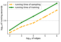
Figure 1. Scalability experiment results on Erdos-Renyi graphs with an average degree of 10.

4.3. Scalability Analysis

To evaluate the scalability of our proposed model, we conduct experiments on Erdos-Renyi graphs with increasing sizes from 100 to 1,000,000 edges, where each node has an average degree of 10. We uniformly split the edges of each graph into 10 different snapshots and learn the temporal graph representations using our model with default parameters. The experiments are conducted on a Lambda Deep Learning 2-GPU Workstation (RTX 2080). As shown in Figure 1, the log-log plot of the running time versus the number of nodes demonstrates that our model’s performance is polynomial in time with respect to the graph’s size. The slopes of the curves are less than 1 in the log-log space, indicating that our method performs in sub-linear time due to its use of parallel processing. Thus, our proposed method can be efficiently scaled to handle large networks commonly found in real-world applications.

5. Conclusion

We introduced a novel dynamic graph-level embedding method based on temporal backtracking random walk. Our method can capture both the structural and evolving information of dynamic graphs. Experimental results on five publicly available datasets for temporal graph similarity ranking show the superiority of our proposed method over several baselines. Moreover, our model is scalable to larger networks, which makes it applicable to real-world scenarios. Our method provides a promising solution for dynamic graph embedding tasks and can be applied to various real-world applications.

References

- (1)
- Adhikari et al. (2018) Bijaya Adhikari, Yao Zhang, Naren Ramakrishnan, and B Aditya Prakash. 2018. Sub2vec: Feature learning for subgraphs. In Pacific-Asia Conference on Knowledge Discovery and Data Mining. Springer, 170–182.
- Bai et al. (2019) Yunsheng Bai, Hao Ding, Yang Qiao, Agustin Marinovic, Ken Gu, Ting Chen, Yizhou Sun, and Wei Wang. 2019. Unsupervised inductive graph-level representation learning via graph-graph proximity. (2019).
- Beladev et al. (2020) Moran Beladev, Lior Rokach, Gilad Katz, Ido Guy, and Kira Radinsky. 2020. tdGraphEmbed: Temporal dynamic graph-level embedding. In Proceedings of the 29th ACM International Conference on Information & Knowledge Management.
- Chen and Koga (2019) Hong Chen and Hisashi Koga. 2019. Gl2vec: Graph embedding enriched by line graphs with edge features. In International Conference on Neural Information Processing. Springer, 3–14.
- Donnat et al. (2018) Claire Donnat, Marinka Zitnik, David Hallac, and Jure Leskovec. 2018. Learning structural node embeddings via diffusion wavelets. In Proceedings of the 24th ACM SIGKDD International Conference on Knowledge Discovery & Data Mining.
- Goyal et al. (2020) Palash Goyal, Sujit Rokka Chhetri, and Arquimedes Canedo. 2020. dyngraph2vec: Capturing network dynamics using dynamic graph representation learning. Knowledge-Based Systems 187 (2020), 104816.
- Goyal et al. (2018) Palash Goyal, Nitin Kamra, Xinran He, and Yan Liu. 2018. Dyngem: Deep embedding method for dynamic graphs. arXiv preprint arXiv:1805.11273 (2018).
- Grover and Leskovec (2016) Aditya Grover and Jure Leskovec. 2016. node2vec: Scalable feature learning for networks. In Proceedings of the 22nd ACM SIGKDD International Conference on Knowledge Discovery and Data Mining. ACM, 855–864.
- Hamilton et al. (2016) William L Hamilton, Jure Leskovec, and Dan Jurafsky. 2016. Diachronic word embeddings reveal statistical laws of semantic change. arXiv preprint arXiv:1605.09096 (2016).
- Kipf and Welling (2016) Thomas N Kipf and Max Welling. 2016. Variational graph auto-encoders. arXiv preprint arXiv:1611.07308 (2016).
- Li et al. (2018) Taisong Li, Jiawei Zhang, S Yu Philip, Yan Zhang, and Yonghong Yan. 2018. Deep dynamic network embedding for link prediction. IEEE Access 6 (2018).
- Narayanan et al. (2017) Annamalai Narayanan, Mahinthan Chandramohan, Rajasekar Venkatesan, Lihui Chen, Yang Liu, and Shantanu Jaiswal. 2017. graph2vec: Learning distributed representations of graphs. arXiv preprint arXiv:1707.05005 (2017).
- Nguyen et al. (2018) Giang Hoang Nguyen, John Boaz Lee, Ryan A Rossi, Nesreen K Ahmed, Eunyee Koh, and Sungchul Kim. 2018. Continuous-time dynamic network embeddings. In Companion Proceedings of the The Web Conference 2018. International World Wide Web Conferences Steering Committee, 969–976.
- Perozzi et al. (2014) Bryan Perozzi, Rami Al-Rfou, and Steven Skiena. 2014. Deepwalk: Online learning of social representations. In Proceedings of the 20th ACM SIGKDD International Conference on Knowledge Discovery and Data Mining. ACM.
- Ribeiro et al. (2017) Leonardo FR Ribeiro, Pedro HP Saverese, and Daniel R Figueiredo. 2017. struc2vec: Learning node representations from structural identity. In Proceedings of the 23rd ACM SIGKDD International Conference on Knowledge Discovery & Data Mining. 385–394.
- Tsitsulin et al. (2018) Anton Tsitsulin, Davide Mottin, Panagiotis Karras, Alexander Bronstein, and Emmanuel Müller. 2018. Netlsd: hearing the shape of a graph. In Proceedings of the 24th ACM SIGKDD International Conference on Knowledge Discovery and Data Mining. 2347–2356.
- Wang et al. (2016) Daixin Wang, Peng Cui, and Wenwu Zhu. 2016. Structural deep network embedding. In Proceedings of the 22nd ACM SIGKDD International Conference on Knowledge Discovery and Data Mining. ACM, 1225–1234.
- Wang et al. (2021a) Lili Wang, Chongyang Gao, Chenghan Huang, Ruibo Liu, Weicheng Ma, and Soroush Vosoughi. 2021a. Embedding Heterogeneous Networks into Hyperbolic Space Without Meta-path. In Proceedings of the AAAI Conference on Artificial Intelligence, Vol. 35. 10147–10155.
- Wang et al. (2021b) Lili Wang, Chenghan Huang, Ying Lu, Weicheng Ma, Ruibo Liu, and Soroush Vosoughi. 2021b. Dynamic Structural Role Node Embedding for User Modeling in Evolving Networks. ACM Trans. Inf. Syst. (2021).
- Wang et al. (2021c) Lili Wang, Chenghan Huang, Weicheng Ma, Xinyuan Cao, and Soroush Vosoughi. 2021c. Graph embedding via diffusion-wavelets-based node feature distribution characterization. In Proceedings of the 30th ACM International Conference on Information & Knowledge Management. 3478–3482.
- Wang et al. (2021d) Lili Wang, Chenghan Huang, Weicheng Ma, Ruibo Liu, and Soroush Vosoughi. 2021d. Hyperbolic node embedding for temporal networks. Data Mining and Knowledge Discovery (2021), 1–35.
- Wang et al. (2021e) Lili Wang, Chenghan Huang, Weicheng Ma, Ying Lu, and Soroush Vosoughi. 2021e. Embedding Node Structural Role Identity Using Stress Majorization. In Proceedings of the 30th ACM International Conference on Information & Knowledge Management.
- Wang et al. (2020) Lili Wang, Ying Lu, Chenghan Huang, and Soroush Vosoughi. 2020. Embedding Node Structural Role Identity into Hyperbolic Space. In Proceedings of the 29th ACM International Conference on Information & Knowledge Management.
- Yu et al. (2017) Wenchao Yu, Charu C Aggarwal, and Wei Wang. 2017. Temporally factorized network modeling for evolutionary network analysis. In Proceedings of the Tenth ACM International Conference on Web Search and Data Mining. 455–464.
- Zhou et al. (2018) Lekui Zhou, Yang Yang, Xiang Ren, Fei Wu, and Yueting Zhuang. 2018. Dynamic network embedding by modeling triadic closure process. In Thirty-Second AAAI Conference on Artificial Intelligence.