AbODE: Ab Initio Antibody Design using Conjoined ODEs

Abstract

Antibodies are Y-shaped proteins that neutralize pathogens and constitute the core of our adaptive immune system. De novo generation of new antibodies that target specific antigens holds the key to accelerating vaccine discovery. However, this co-design of the amino acid sequence and the 3D structure subsumes and accentuates, some central challenges from multiple tasks including protein folding (sequence to structure), inverse folding (structure to sequence), and docking (binding).

We strive to surmount these challenges with a new generative model AbODE that extends graph PDEs to accommodate both contextual information and external interactions. Unlike existing approaches, AbODE  uses a single round of full-shot decoding, and elicits continuous differential attention that encapsulates, and evolves with, latent interactions within the antibody as well as those involving the antigen. We unravel fundamental connections between AbODE  and temporal networks as well as graph-matching networks. The proposed model significantly outperforms existing methods on standard metrics across benchmarks.

1 Introduction

Machine learning methods have recently enabled exciting developments for computational drug design, including, on tasks such as protein folding (Jumper et al., 2021), i.e., predicting the 3D structure of a given protein from its amino acid sequence; sequence design or inverse folding (Ingraham et al., 2019b), i.e., generating new sequences that fold into a given 3D structure; and docking (Ganea et al., 2021), i.e., predicting the complex when two proteins bind together.

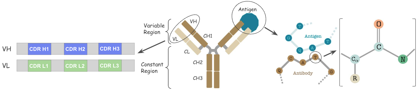
Figure 1: Schematic showing the structure of a residue (amino acid), where the backbone atoms we use are $N$, $C_{\alpha}$ and $C$ (right) and the structure of the antibody (left) which is Y-shaped showing the VH/VL sequences and binding to the antigen, and we focus on CDRs of the variable domain in the heavy chain (VH).

We focus on the problem of antibody design. Antibodies, the versatile Y-shaped proteins that guard against pathogens such as bacteria and viruses, are essential to our adaptive immune mechanism. Typically, an antibody acts by binding to a specific molecule of the pathogen, namely, the antigen. Each antibody recognizes a unique antigen, and the so-called Complementarity Determining Regions (CDRs) at the tip of the antibody determines this specificity (Figure 1). Thus, automating the design of antibodies against specific pathogens (e.g., the SARS-CoV-2 virus) can revolutionize drug discovery (Pinto et al., 2020; Jin et al., 2022b).

Our objective is to co-design the CDR sequence and structure from scratch, conditioned on an antigen. However, significant challenges must be overcome in this pursuit. While recent generative methods for protein sequence design have been successful (Ingraham et al., 2019b), they crucially utilize that the long term dependencies in sequence are local in the 3D space. However, the CDR structures are seldom known a priori, thereby limiting the scope of such approaches (Jin et al., 2022b). In principle, one could segregate the design of sequence from structure. Indeed, once a CDR sequence is generated, folding methods such as AlphaFold that exploit alignment with a family of protein sequences (Jumper et al., 2021) can be employed to estimate the 3D structure of the CDR. However, generating sequence without conditioning on the structure (Alley et al., 2019; Shin et al., 2021a) is known to produce sub-optimal sequences. Moreover, related sequences may be unavailable for scenarios that diverge considerably from naturally occurring antibodies (Ingraham et al., 2019b). Finally, finding antibodies that have a good binding affinity with the target antigens (Raybould et al., 2019) requires search in a huge space ($\sim 20^{60}$ possible CDR sequences).

Initial approaches for antibody design (Pantazes & Maranas, 2010; Li et al., 2014; Lapidoth et al., 2015; Adolf-Bryfogle et al., 2018) relied on hand-crafted energy functions that entailed expensive simulation, and could not sufficiently capture complex interactions  (Graves et al., 2020). Going beyond 1D sequence prediction (Alley et al., 2019; Shin et al., 2021a; Saka et al., 2021a; Akbar et al., 2022), recent generative methods co-design structure and sequence (Jin et al., 2022b) and can incorporate information about antigen directly in the model (Jin et al., 2022a; Kong et al., 2023).

Certain shortcomings, however, accompany these advances. The autoregressive scheme (one residue at a time) adopted by (Jin et al., 2022a, b) is susceptible to issues such as vanishing or exploding gradients during training, as well as slow generation and accumulation of errors during inference. Kong et al. (2023) advocate multiple full-shot rounds to address this issue; however, segregating context (intra-antibody) from external interactions (antibody-antigen) precludes joint optimization, and may result in sub-optimality.

We circumvent these issues with a novel viewpoint that models the antibody-antigen complex as a joint 3D graph with heterogeneous edges. Different from all prior works, this perspective allows us to formulate a coupled neural ODE system over the nodes pertaining to the antibody, while simultaneously accounting for the antigen. Specifically, we associate local densities (one per antibody node) that are progressively refined toward globally aligned densities based on simultaneous feedback from the antigen as well as the (other) antibody nodes. The 3D coordinates and the node labels for the antibody can then be sampled after a few rounds in one-shot, i.e., all at once. Thus, the entire procedure is efficient and end-to-end trainable.

We show how invariance can be built in readily into the proposed method AbODE  toward representations that account for rotations and other symmetries. AbODE  establishes a new state-of-the-art (SOTA) for antibody design across standard metrics on several benchmarks. Interestingly, it turns out that it shares connections with two recent methods for equivariant molecular generation and docking, namely, ModFlow and IEGMN. While ModFlow can be recovered as a special case of the AbODE  formulation, IEGMN may be interpreted as a discrete analog of AbODE. One one hand, these similarities reaffirm the kinship of different computational drug design tasks; on the other, they suggest the broader applicability of neural PDEs as effective tools for these tasks. Our experiments further reinforce this phenomenon: AbODE  is already competitive with the SOTA methods on a task it is not tailored for, namely, fixed backbone protein sequence design.

1.1 Contributions

In summary, we make following contributions.

• We propose AbODE, a generative model that extends graph PDEs by jointly modeling the internal context and interactions with external objects (e.g., antigens).

• AbODE  co-designs the antibody sequence and structure, using a single round of full-shot decoding.

• Empirically,  AbODE  registers SOTA performance on various sequence design and structure prediction tasks.

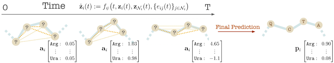
Figure 2: A demonstration of AbODE. The initial structure and amino acid labels evolve in time under $f_{\psi}$ and are subsequently transformed into a final structure and amino acid labels.

2 Related Work

Antibody/protein design

Early approaches for computational antibody design optimize hand-crafted energy functions (Pantazes & Maranas, 2010; Li et al., 2014; Lapidoth et al., 2015; Adolf-Bryfogle et al., 2018). These methods require costly simulations and are prone to defects due to complex interactions between chains that cannot be captured by force fields or statistical functions (Graves et al., 2020). Recently, deep generative models have been utilized for 1D sequence prediction in proteins (O’Connell et al., 2018; Ingraham et al., 2019b; Strokach et al., 2019; Karimi et al., 2020; Cao et al., 2021; Dauparas et al., 2022) and antibodies (Alley et al., 2019; Shin et al., 2021a; Saka et al., 2021a; Akbar et al., 2022), conditioned on the backbone 3D structure. Jin et al. (2022b) proposed to co-design the sequence and structure via an autoregressive refinement technique, while Kong et al. (2023) advocated multiple rounds of full-shot decoding together with an encoder for intra-antibody context, and a separate encoder for external interactions.

Different from all these works, we formulate a single full-shot method that extends graph PDEs(Chamberlain et al., 2021; Iakovlev et al., 2020) to accommodate and condition on spatial and context-based information of the antigen, tailored to antibody sequence and structure generation.

Generative models for graphs

Our work is related to continuous time models for graph generation (Verma et al., 2022; Avelar et al., 2019) that incorporate dynamic interactions (Chen et al., 2018; Grathwohl et al., 2018; Iakovlev et al., 2020; Eliasof et al., 2021) over graphs. Methods have also been developed for protein structure generation, e.g., Folding Diffusion (Wu et al., 2022), Anand & Huang (2018), AlphaDesign (Gao et al., 2022), etc. Most of these methods lack the flexibility to be directly applied to antibody sequence and structure design, due to their inability to capture effective inductive biases, conditional information, and higher-order features. In contrast, we can combine conditional information and evolve the structure and sequence via latent co-interacting trajectories.

3D structure prediction

Our method is also closely related to docking  (Ganea et al., 2021; Stärk et al., 2022) and protein folding (Ingraham et al., 2019c, d; Baek et al., 2021; Jumper et al., 2021; Ingraham et al., 2022). Methods like DiffDock (Corso et al., 2023) and EquiBind (Stärk et al., 2022) predict only the structure of the molecule given a protein binding site but lack any generative component related to sequence design. AlphaFold (Jumper et al., 2021) requires holistic information like protein sequence, multi-sequence alignment (MSA), and template features. These models cannot be directly applied for antibody design, where MSA is not specified in advance and one needs to predict the structure of an incomplete sequence. In contrast, we learn to co-model the 3D structure and sequence for incomplete graphs and interleave structure modeling with sequence prediction.

3 Antibody sequence and structure co-design

An antibody (Ab) is a Y-shaped protein (Fig. 1) that identifies antigens of a foreign object (e.g., a virus) and stimulates an immunological response. An antibody consists of a constant domain, and a symmetric variable region divided into heavy (H) and light (L) chains (Kuroda et al., 2012). The surface of the antibody contains three complementarity-determining regions (CDRs), which act as the main binding determinant. CDR-H3 makes up the majority of the binding affinity (Fischman & Ofran, 2018). The non-CDR regions are highly preserved (Kuroda et al., 2012); thus, it is common to formulate antibody design as a CDR design problem (Shin et al., 2021b).

We view the antibody-antigen complex as a joint graph with interactions between nodes across the binding. We co-model both the sequence and the 3D conformation of the CDR regions with a graph PDE and apply our method to antigen-specific and unconditional antibody design tasks.

We seek a representation that is invariant to translations and rotations due to its locality along the backbone. Moreover, we would like the edge features to be sufficiently informative such that the relative neighborhoods can be reconstructed up to rigid body motion (Ingraham et al., 2019b). We describe next a representation that satisfies these desiderata.

3.1 The antibody-antigen graph

We define the antigen-antibody complex as a 3D graph $G=(V,E,X)$, with antibody Ab and antigen Ag vertices $V=(V_{\texttt{Ab}},V_{\texttt{Ag}})$, coordinates $X=(X_{\texttt{Ab}},X_{\texttt{Ag}})$ and edges $E=(E_{\texttt{Ab}},E_{\texttt{Ab-Ag}})$ within the antibody as well as between the antibody and the antigen. Each vertex $v\in\mathcal{A}=\{\texttt{Arg},\texttt{His},\ldots\}$ is one of 20 amino acids. We treat the labels with a Categorical distribution, such that the label features $\mathbf{a}_{i}\in\mathrm{R}^{20}$ represent the unnormalized amino acid probabilities. We also represent each residue by the cartesian 3D coordinates of its three backbone atoms $\{N,C_{\alpha},C\}$ (see Fig. 1). For the $i^{th}$ residue $\mathbf{x}_{i}$ we compute its spatial features $\mathbf{s}_{i}=(r_{i},\alpha_{i},\gamma_{i})$ in Eq. 1, where, $r_{i}$ denotes the distance between consecutive residues $x_{i}$ and $x_{i+1}$, $\alpha_{i}$ is the co-angle of residue $i$ wrt previous and next residue, $\gamma_{i}$ is the azimuthal angle of $i$’s local plane, and $\mathbf{n}_{i}$ is the normal vector. The full residue state $\mathbf{z}_{i}=[\mathbf{a}_{i},\mathbf{s}_{i}]$ concatenates the label features $\mathbf{a}_{i}$ and the spatial features $\mathbf{s}_{i}$.

$$r_{i} =\left\|\mathbf{u}_{i}\right\|,\quad\mathbf{u}_{i}=\mathbf{x}_{i+1}-\mathbf{x}_{i}$$ (1)

$$\alpha_{i} =\cos^{-1}\left(\frac{\left\langle\mathbf{u}_{i},\mathbf{u}_{i-1}\right\rangle}{\left\|\mathbf{u}_{i}\right\|\cdot\left\|\mathbf{u}_{i-1}\right\|}\right)$$ (2)

$$\gamma_{i} =\cos^{-1}\left(\frac{\left\langle\mathbf{u}_{i},\mathbf{n}_{i}\right\rangle}{\left\|\mathbf{u}_{i}\right\|\cdot\left\|\mathbf{n}_{i}\right\|}\right),\quad\mathbf{n}_{i}=\mathbf{u}_{i}\times\mathbf{u}_{i-1}.$$ (3)

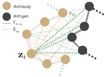
Figure 3: Schematic graph construction for the antigen-antibody complex with internal edges $E_{\texttt{Ab}}$ and external edges $E_{\texttt{Ab-Ag}}$. In the unconditional setting (i.e., the antigen is not specified), this reduces to an antibody graph

Interactions

To capture the interactions pertaining to the complex, we define edges $E_{\texttt{Ab}}$ between all antibody residues and edges $E_{\texttt{Ab-Ag}}$ between all antibody and antigen residues (See Figure 3). We also define edge features between nodes $i$ and $j$,

$$\mathbf{e}_{ij}=( \Delta\mathbf{z}_{ij},i-j,\operatorname{RBF}\left(\left\|\mathbf{s}_{i}-\mathbf{s}_{j}\right\|\right).$$ (4)

$$\mathcal{O}_{i}^{\top}\frac{s_{i,\alpha}-s_{j,\alpha}}{\left\|s_{i,\alpha}-s_{j,\alpha}\right\|},\mathcal{O}_{i}^{\top}\mathcal{O}_{j},k_{ij}).$$ (5)

These include state differences $\Delta\mathbf{z}_{ij}=\{\Delta\mathbf{a}_{ij},\Delta\mathbf{s}_{ij}\}$ over label features $\Delta\mathbf{a}_{ij}=\mathbf{a}_{j}-\mathbf{a}_{i}$ and spatial features $\Delta\mathbf{s}_{ij}=\{(\Delta r_{ij},\Delta\alpha_{ij},\Delta\gamma_{ij})_{p}\mid p\in\{N,C_{\alpha},C\}\}$, backbone distance $i-j$, and spatial distance $\texttt{RBF}(||\mathbf{s}_{i}-\mathbf{s}_{j}||)$ (here, RBF is the standard radius basis function kernel). The fourth term encodes directional embedding in the relative direction of $j$ in the local coordinate frame $\mathcal{O}_{i}$ (Ingraham et al., 2019b), and the $\mathcal{O}^{T}_{i}\mathcal{O}_{j}$ describes the orientation encoding of the node $i$ with node $j$ (See Appendix A.1 for details). Finally, we encode within-antibody edges with $k=1$ and antibody-antigen edges with $k=2$.

Task formulation

Given a three-dimensional antibody or antibody-antigen graph, we aim to learn a PDE in order to generate an amino acid sequence and the corresponding 3D conformation jointly.

Table 1: AbODE  as a variant of Independent E(3)-Equivariant Graph Matching Network (IEGMN) applied to interactions among two graphs $G_{1}=(V_{1},E_{1})$ and $G_{2}=(V_{2},E_{2})$. Here, $e_{ij}\in E_{1}\cup E_{2}$; $n\in V_{1}\cup V_{2}$; $\texttt{RBF}(\mathbf{x}_{i},\mathbf{x}_{j};\sigma)=\texttt{exp}(-||\mathbf{x}_{i}^{(l)}-\mathbf{x}_{j}^{(l)}||^{2}/\sigma)$; $h_{n}$ and $x_{n}$ denote, respectively, the node embedding and the spatial embedding; $a_{ij}$ are attention based coefficients; $\phi^{x}$ is a real-valued (scalar) parametric function; $\phi^{h,e}$ are parametric functions (MLPs); $\textbf{f}_{ij},\textbf{f}_{i}$ are the original edge and node features; $\beta,\eta$ are scaling parameters and $\mathbf{W}$ is a learnable matrix. For AbODE , $\alpha_{i,j}$ are the attention coefficients; $\mathbf{W}_{1},\ldots,\mathbf{W}_{6}$ are learnable weight parameters; $d$ is the hidden size of each head; $\mathcal{N}_{int}(i)$ are the neighbours $j$ of node $i$ such that $k_{ij}=1$, and $\mathcal{N}_{ext}(i)$ are the neighbours such that $k_{ij}=2$.

Method	IEGMN layer	AbODE
Edge	$\mathbf{m}_{ij}=\varphi^{e}\left(\mathbf{h}_{i}^{(l)},\mathbf{h}_{j}^{(l)},\operatorname{RBF}\left(\mathbf{x}_{i}^{(l)},\mathbf{x}_{j}^{(l)};\sigma\right),\mathbf{f}_{ij}\right)$	$\alpha_{i,j}=\operatorname{softmax}\left(\frac{(\mathbf{W}_{3}\mathbf{z}_{i})^{\top}(\mathbf{W}_{4}\mathbf{z}_{j}+\mathbf{W}_{6}\mathbf{e}_{i,j}).}{\sqrt{d}}\right)$
	$\mathrm{m}_{n}=\frac{1}{|\mathcal{N}(n)|}\sum_{j\in\mathcal{N}(n)}\mathrm{m}_{nj}$	$m_{i}^{\prime}=\sum_{j\in\mathcal{N}_{i}}\alpha_{i,j}\left(\mathbf{W}_{2}\mathbf{z}_{j}+\mathbf{W}_{6}\mathbf{e}_{ij}\right)$
Intra and Inter connections	$\bm{\mu}_{ij}=a_{ij}\mathbf{Wh}_{j}^{(l)},\forall i\in\mathcal{V}_{1},j\in\mathcal{V}_{2}\text{ or }i\in\mathcal{V}_{2},j\in\mathcal{V}_{1}$	$m_{ij}^{\prime,ext}=\alpha_{i,j}\left(\mathbf{W}_{2}\mathbf{z}_{j}+\mathbf{W}_{6}\mathbf{e}_{ij}\right),~{}m_{ij}^{\prime,int}=\alpha_{i,j}\left(\mathbf{W}_{2}\mathbf{z}_{j}+\mathbf{W}_{6}\mathbf{e}_{ij}\right)$
	$\bm{\mu}_{i}=\sum_{j\in\mathcal{V}_{2}}\bm{\mu}_{ij},\forall i\in\mathcal{V}_{1},\quad\bm{\mu}_{k}=\sum_{l\in\mathcal{V}_{1}}\bm{\mu}_{kl},\forall k\in\mathcal{V}_{2}$	$\textbf{m}_{i}^{\prime,int}=\sum_{j}^{\mathcal{N}_{int}(i)}m_{ij}^{\prime,int},~{}\textbf{m}_{i}^{\prime,ext}=\sum_{j}^{\mathcal{N}_{ext}(i)}m_{ij}^{\prime,ext}$
Node embedding	$\mathbf{h}_{n}^{(l+1)}=(1-\beta)\cdot\mathbf{h}_{n}^{(l)}+\beta\cdot\varphi^{h}\left(\mathbf{h}_{n}^{(l)},\mathbf{m}_{n},\bm{\mu}_{n},\mathbf{f}_{n}\right)$	$\mathrm{a}_{i}^{\prime}=\mathbf{W}_{1}\mathbf{a}_{i}+\mathbf{m}_{i}^{\prime,\text{int}}+\mathbf{m}_{i}^{\prime,\text{ext}}$
Coordinate embedding	$\mathbf{x}_{n}^{(l+1)}=\eta\mathbf{x}_{n}^{(0)}+(1-\eta)\mathbf{x}_{n}^{(l)}+\sum_{j\in\mathcal{N}(n)}\left(\mathbf{x}_{n}^{(l)}-\mathbf{x}_{j}^{(l)}\right)\varphi^{x}\left(\mathbf{m}_{nj}\right)$	$\mathrm{s}_{i}^{\prime}=\mathbf{W}_{1}\mathbf{s}_{i}+\mathbf{m}_{i}^{\prime,\text{int}}+\mathbf{m}_{i}^{\prime,\text{ext}}$

3.2 Conjoined system of ODEs

We propose to model the distribution of antibody-antigen complexes by a differential graph flow $\mathbf{z}(t)$ over time $t\in\mathrm{R}_{+}$. We initialize the initial state $\mathbf{z}(0)$ to a uniform categorical vector, similar to mask initialization (Jin et al., 2022b; Kong et al., 2023). Coordinates are initialized with the even distribution between the residue right before CDRs and the one right after CDRs following (Kong et al., 2023), and we learn a differential $\frac{d\mathbf{z}(t)}{dt}$ that maps to the end state $\mathbf{z}(T)$ that matches data.

We begin by assuming an ODE system $\{\mathbf{z}_{i}(t)\}$ over time $t\in\mathrm{R}_{+}$, where node the time evolution of node $i$ is an ODE

$$\dot{\mathbf{z}}_{i}(t)=\frac{\partial\mathbf{z}_{i}(t)}{\partial t}=f_{\psi}(t,\mathbf{z}_{i}(t),\mathbf{z}_{N(i)}(t),\{\mathbf{e}_{ij}(t)\}_{j})$$ (6)

where $N(i)=\{j~{}:~{}(i,j)~{}\in~{}E\}$ indexes the neighbors of node $i$, and the function $f$ parameterized by $\psi$ is our main learning goal. The differentials form a coupled ODE system

$$\dot{\mathbf{z}}(t) =\begin{pmatrix}\dot{\mathbf{z}}_{1}(t)\\ \vdots\\ \dot{\mathbf{z}}_{M}(t)\end{pmatrix}$$ (7)

$$=\begin{pmatrix}f_{\psi}(t,\mathbf{z}_{1}(t),\mathbf{z}_{N(1)}(t),\{\mathbf{e}_{1j}(t)\}_{j})\\ \vdots\\ f_{\psi}(t,\mathbf{z}_{M}(t),\mathbf{z}_{N(M)}(t),\{\mathbf{e}_{Mj}(t)\}_{j})\big{)}\end{pmatrix}$$ (8)

$$\mathbf{z}(T) =\mathbf{z}(0)+\int_{0}^{T}\dot{\mathbf{z}}(t)dt~{}.$$ (9)

where $M$ is the number of nodes. The above ODE system corresponds to a graph PDE (Iakovlev et al., 2020; Verma et al., 2022), whose forward pass and backpropagation can be solved efficiently by ODE solvers.

Interestingly, it turns out that the PDE about a recently proposed method for molecular generation can be recovered as a particular case of 7, when all the edges are set to be of the same type.

Proposition 1

: ModFlow (Verma et al., 2022) can be seen as a special case of AbODE  in an unconditional setting. This can be achieved by setting $k_{ij}=1$ for every $e_{ij}$.

3.3 Attention-based differential

We capture the interactions between the antigen and antibody residues with graph attention (Shi et al., 2020)

$$\alpha_{ij} =\operatorname{softmax}\left(\frac{\left(\mathbf{W}_{3}\mathbf{z}_{i}\right)^{\top}\left(\mathbf{W}_{4}\mathbf{z}_{j}+\mathbf{W}_{6}\mathbf{e}_{ij}\right)}{\sqrt{d}}\right)$$ (10)

$$\mathbf{z}_{i}^{\prime} =\mathbf{W}_{1}\mathbf{z}_{i}+\sum_{j\in N(i)}\alpha_{ij}\left(\mathbf{W}_{2}\mathbf{z}_{j}+\mathbf{W}_{6}\mathbf{e}_{ij}\right)$$ (11)

where $\textbf{W}_{1},\ldots,\textbf{W}_{6}$ are weight parameters and $d$ is the head size. The $\alpha$’s are the attention coefficients corresponding to within and across edges, which are used to update the node feature $\mathbf{z}_{i}$. Interestingly, our method also shares similarities with the Independent E(3)-Equivariant Graph Matching Networks (IEGMNs) for docking (Ganea et al., 2021).

Proposition 2

: AbODE  can be cast as Independent E(3)- Equivariant Graph Matching Networks (IEGMN) (Ganea et al., 2021)). The operations are listed in Table 1 (See Appendix A.2 for more details).

In this sense, our extended graph PDE unifies molecular generation and docking with protein/antibody design.

We now describe our training objective.

Table 2: Top: Unconditional sequence and structure benchmark. We report perplexity (PPL) and root mean square deviation (RMSD) for each CDR in the heavy chain. Baselines are from Jin et al. (2022b). Bottom: Antigen-conditional sequence and structure benchmark on SAbDab (Dunbar et al., 2014). We report amino acid recovery (AAR) and root mean square deviation (RMSD) for each CDR in the heavy chain. Baselines are from Kong et al. (2023).

	CDR-H1		CDR-H2		CDR-H3
Method	PPL ($\downarrow$)	RMSD ($\downarrow$)	PPL ($\downarrow$)	RMSD ($\downarrow$)	PPL ($\downarrow$)	RMSD ($\downarrow$)
LSTM	$6.79$	(N/A)	$7.21$	(N/A)	$9.70$	(N/A)
AR-GNN	$6.44$	$2.97$	$6.86$	$2.27$	$9.44$	$3.63$
RefineGNN	$6.09$	$1.18$	$6.58$	$0.87$	$8.38$	$2.50$
AbODE	$4.25$ $\pm$ $0.46$	$0.73$ $\pm$ $0.15$	$4.32$ $\pm$ $0.32$	$0.63$ $\pm$ $0.19$	$6.35$ $\pm$ $0.29$	$2.01$ $\pm$ $0.13$

	CDR-H1		CDR-H2		CDR-H3
Method	AAR $\%$ ($\uparrow$)	RMSD ($\downarrow$)	AAR $\%$ ($\uparrow$)	RMSD ($\downarrow$)	AAR $\%$ ($\uparrow$)	RMSD ($\downarrow$)
LSTM	40.98 $\pm$ 5.20	(N/A)	28.50 $\pm$ 1.55	(N/A)	15.69 $\pm$ 0.91	(N/A)
C-LSTM	40.93 $\pm$ 5.41	(N/A)	29.24 $\pm$ 1.08	(N/A)	15.48 $\pm$ 1.17	(N/A)
RefineGNN	39.40 $\pm$ 5.56	3.22 $\pm$ 0.29	37.06 $\pm$ 3.09	3.64 $\pm$ 0.40	21.13 $\pm$ 1.59	6.00 $\pm$ 0.55
C-RefineGNN	33.19 $\pm$ 2.99	3.25 $\pm$ 0.40	33.53 $\pm$ 3.23	3.69 $\pm$ 0.56	18.88 $\pm$ 1.37	6.22 $\pm$ 0.59
MEAN	58.29 $\pm$ 7.27	0.98 $\pm$ 0.16	47.15 $\pm$ 3.09	0.95 $\pm$ 0.05	36.38 $\pm$ 3.08	2.21 $\pm$ 0.16
AbODE	70.5 $\pm$ 1.14	0.65 $\pm$ 0.1	55.7 $\pm$ 1.45	0.73 $\pm$ 0.14	39.8 $\pm$ 1.17	1.73 $\pm$ 0.11

3.4 Training Objective

We optimize for the data fit of the generated states z(T) given by the differential function $f_{\psi}$. The loss consists of two components: one for the sequence and another for the structure

$$\mathcal{L}=\mathcal{L}_{\texttt{seq}}+\mathcal{L}_{\texttt{structure}}$$ (12)

The sequence loss is quantified in terms of the cross-entropy between the true label $\mathbf{a}_{ni}^{\texttt{true}}$ and the label distribution $\mathbf{a}_{ni}$predicted by the model, i.e.,

$$\mathcal{L}_{\texttt{seq}}=\frac{1}{N}\sum_{n=1}^{N}\frac{1}{M}\sum_{i=1}^{M_{i}}\mathrm{CE}\left(\mathbf{a}_{ni}^{\text{true }},\mathbf{a}_{ni}\right)$$ (13)

where $n$ indexes the $N$ datapoints and $i$ indexes the $M_{i}$ residues. The structure loss is computed based on the fit to the data sample in terms of the angles and radii:

$$\mathcal{L}_{\texttt{structure}}=\frac{1}{N}\sum_{n=1}^{N}\frac{1}{M}\sum_{i=1}^{M_{i}}\lambda\left(\mathcal{L}_{\texttt{angle}}^{ni}+\mathcal{L}_{\texttt{radius}}^{ni}\right).$$ (14)

For each residue angle pair $(\alpha,\gamma)$ we compute the negative log of the von-Mises likelihood

$$\mathcal{L}_{\texttt{angle}}^{ni}=\sum_{k}^{\left\{\mathrm{C}_{\alpha},\mathrm{C},\mathrm{N}\right\}}\sum_{\theta\in\{\alpha,\gamma\}}\log\mathcal{M}\left(\theta_{ik}^{n}\mid\theta_{ik}^{n,\text{ true }},\kappa\right)$$ (15)

where $\kappa$ is a scale parameter, and $k$ is atom index. The von Mises distribution can be interpreted as a Gaussian distribution over the domain of angles. On the other hand, the radius loss is the negative log of a Gaussian distance.

$$\mathcal{L}_{\texttt{radius}}^{ni}=\sum_{k}^{\left\{\mathrm{c}_{\alpha},\mathrm{C},\mathrm{N}\right\}}\log\mathcal{N}\left(r_{ik}^{n}\mid r_{ik}^{n,\text{ true }},\sigma_{r}^{2}\right)$$ (16)

where $\sigma_{r}^{2}$ is the radius variance. Note that our method predicts the sidechain spatial coordinates, also used to calculate the total loss. Here $\lambda$ is the polar loss weight, set to $\lambda=0.8$. We set $\kappa=10$, $\sigma_{r}^{2}=0.1$ to prefer narrow likelihoods for accurate structure prediction.

We next describe the generation step.

3.5 Sequence and structure prediction

Given the antibody or antigen-antibody complex, we generate an antibody sequence and the corresponding structure by solving the system of ODEs as described in section 3.2 for time T to obtain $\mathbf{z}(T)=[\mathbf{a}(T),\mathbf{s}(T)]$. Using the softmax operator, we transform the label features $\mathbf{a}(T)$ into Categorical amino acid probabilities p. We pick the most probable amino acid per node. A schematic representation is shown in Fig. 2

4 Experiments

Tasks

We benchmark AbODE on a series of challenging tasks: (i) we evaluate the model on unconditional antibody sequence and structure generation against ground truth structures in the Structural Antibody Database SAbDab (Dunbar et al., 2014) section 4.1, (ii) we benchmark our method in terms of its ability to generate antigen-conditioned anti- body sequences and structures from SAbDab in section 4.2, (iii) we evaluate our model on the task of designing CDR- H3 over 60 manually selected diverse complexes (Adolf-Bryfogle et al., 2018) in section 4.3, (iv) we extend our model to incorporate information about the constant region of the antibody in section 4.4, and finally, (v) we extend AbODE to de novo protein sequence design with a fixed backbone in section 4.5.

Baselines

We compare AbODE  with the state-of-the-art baseline methods. On the uncontrolled generation task, we compare against sequence-only LSTM (Saka et al., 2021b; Akbar et al., 2022), an autoregressive graph network AR- GNN (You et al., 2018) tailored for antibodies, and an autoregressive method RefineGNN (Jin et al., 2022b), which considers the 3D geometry and co-models the sequence and the structure.

On the antigen-conditioned sequence and structure genera- tion task, we again compare against LSTM and RefineGNN. We also consider their variants C-LSTM and C-RefineGNN proposed in Kong et al. (2023), where they adapt the current methodology to consider the entire context of the antibody-antigen complex. We additionally consider MEAN (Kong et al., 2023) which uses progressive decoding to generate CDR by encoding the external antigen context of 1D/3D information. Finally, we also compare against a physics-based simulator RosettaAD (Adolf-Bryfogle et al., 2018).

Implementation

AbODE is implemented in PyTorch (Paszke et al., 2019). We used three layers of a Transformer Convolutional Network (Shi et al., 2020) with embedding dimensions of $128-256-64$. Our models were trained with the Adam optimizer for 5000 epochs using batch size 300. For details, we refer the reader to Appendix A.3.

Table 3: Top: Adding constant region information for unconditioned sequence and structure modeling task. Bottom: Adding constant region information for antigen-conditioned antibody sequence and structure modeling task.

	CDR-H1		CDR-H2		CDR-H3
AbODE	PPL ($\downarrow$)	RMSD ($\downarrow$)	PPL ($\downarrow$)	RMSD ($\downarrow$)	PPL ($\downarrow$)	RMSD ($\downarrow$)
$-$ Constant Region	4.25 $\pm$ 0.46	0.73 $\pm$ 0.15	4.32 $\pm$ 0.32	0.63 $\pm$ 0.19	6.35 $\pm$ 0.29	2.01 $\pm$ 0.13
$+$ Constant Region ($z_{<i}$)	4.31 $\pm$ 0.31	0.69 $\pm$ 0.21	4.17 $\pm$ 0.29	0.59 $\pm$ 0.21	6.41 $\pm$ 0.37	1.94 $\pm$ 0.17

	CDR-H1		CDR-H2		CDR-H3
AbODE	AAR $\%$ ($\uparrow$)	RMSD ($\downarrow$)	AAR $\%$ ($\uparrow$)	RMSD ($\downarrow$)	AAR $\%$ ($\uparrow$)	RMSD ($\downarrow$)
$-$ Constant Region	70.5 $\pm$ 1.14	0.65 $\pm$ 0.1	55.7 $\pm$ 1.45	0.73 $\pm$ 0.14	39.8 $\pm$ 1.17	1.73 $\pm$ 0.11
$+$ Constant Region ($z_{<i}$)	71.9 $\pm$ 1.87	0.71 $\pm$ 0.23	56.8 $\pm$ 1.97	0.70 $\pm$ 0.14	36.7 $\pm$ 1.5	1.88 $\pm$ 0.11

4.1 Unconditioned Sequence and Structure Modeling

Data

We obtained the antibody sequences and structure from Structural Antibody Database (SAbDab) (Dunbar et al., 2014) and removed any incomplete or redundant complexes. We followed a similar strategy to Jin et al. (2022b), where we focus on generating heavy chain CDRs, and curated the dataset by clustering the CDR sequences via MMseq2 (Steinegger & Söding, 2017) with $40\%$ sequence identity. We then randomly split the clusters into training, validation, and test sets with an 8:1:1 ratio.

Metrics

We evaluate our method on perplexity (PPL) and root mean square deviation (RMSD) between the predicted structures and the ground truth structures on the test data. We report the results for all the CDR-H regions. We calculate the RMSD by the Kabsch algorithm (Kabsch, 1976) based on $C_{\alpha}$ spatial features of the CDR residues.

Results

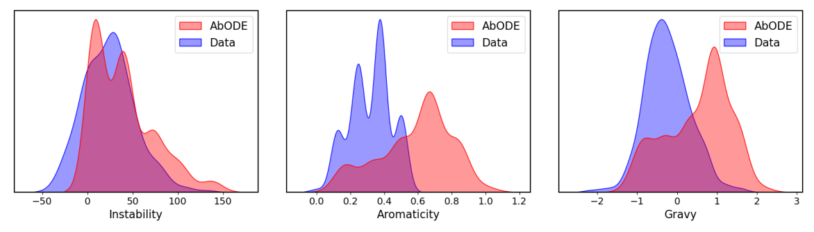
Figure 4: Functional evaluation of generated antibodies vs. data for CDR-H1 unconditional antibody sequence and structure design

The LSTM baselines do not involve structure prediction, so we only report the RMSD for the graph-based method. Table 2 reports the performance of AbODE  on uncontrolled generation, where AbODE  outperforms all the baselines on both metrics. Notably, AbODE  significantly reduces the PPL in all CDR regions and typically predicts a structure close to the ground truth structure. We also evaluate the biological functionality of the generated antibodies, shown in Fig. 4. Specifically, we considered the following properties:

• Gravy: The Gravy value is calculated by adding the hydropathy value for each residue and dividing it by the length of the sequence (Kyte & Doolittle, 1982)

• Instability: The Instability index is calculated using the approach of Guruprasad et al. (1990), which predicts regional instability of dipeptides that occur more frequently in unstable proteins when compared to stable proteins.

• Aromaticity: It calculates the aromaticity value of a protein according to Lobry & Gautier (1994). It is simply the relative frequency of Phe+Trp+Tyr.

As our plots demonstrate, AbODE can essentially replicate the behavior of the data in terms of instability and gravy. However, there is some discrepancy in terms of spread concerning aromaticity.

4.2 Antigen Conditioned Sequence and Structure Modeling

Data

We took the antigen-antibody complexes dataset from Structural Antibody Database (Dunbar et al., 2014) and removed the illegal data points, renumbering them to the IMGT scheme (Lefranc et al., 2003). We follow the data preparation strategy of Kong et al. (2023); Jin et al. (2022b) by splitting the dataset into training, validation, and test sets. We accomplish this by clustering the sequences via MMseq2 (Steinegger & Söding, 2017) with $40\%$ sequence identity. Then we split all clusters into training, validation, and test sets in the proportion 8:1:1.

Metrics

We employ Amino Acid Recovery (AAR) and RMSD for quantitative evaluation. AAR is defined as the overlapping rate between the predicted 1D sequences and the ground truth. RMSD is calculated via the Kabsch algorithm (Kabsch, 1976) based on $C_{\alpha}$ spatial features of the CDR residues.

Results

Table 2 shows the performance of AbODE  compared to the baseline methods. AbODE  is able to perform better than other competing methods in terms of structure and sequence prediction. AbODE  is able to improve over the SOTA by directly combining the antibody context with the information about the antigen via the attention network, thereby demonstrating the benefits of joint modeling. As a result, AbODE  able to learn the underlying distribution of the complexes effectively.

Table 4: Perplexity (PPL) and Amino Acid Recovery (AAR) for different methods on fixed backbone sequence design task. Baselines are from Shi et al. (2023).

	PPL ($\downarrow$)			AAR $\%$ ($\uparrow$)
Method	Short	Single-chain	All	Short	Single-chain	All
GVP-Transformer	$8.94$	$8.67$	$6.70$	$27.3$	$28.3$	$36.5$
Structured GNN	$8.31$	$8.88$	$6.55$	$28.4$	$28.1$	$37.3$
GVP-GNN	$7.10$	$7.44$	$5.29$	$32.1$	$32.0$	$40.2$
ProtSeed	$7.32$	$7.38$	$5.60$	$34.8$	$34.1$	$43.8$
AbODE	$7.19$ $\pm$ $0.34$	$7.33$ $\pm$ $0.25$	$5.85$ $\pm$ $0.45$	$34.4$ $\pm$ $1.7$	$34.7$ $\pm$ $1.2$	$42.7$ $\pm$ $1.9$

4.3 Antigen-Binding CDR-H3 Design

In order to further evaluate our model, we designed CDR- H3 that binds to a given antigen. We used AAR and RMSD as our scoring metrics. We included RosettaAD (Adolf-Bryfogle et al., 2018), a conventional physics-based baseline for comparison. We benchmark our method on 60 diverse complexes selected by (Adolf-Bryfogle et al., 2018).

Note, however, that the training is still conducted on the SAbDab dataset as described in section 4.2, where we eliminate the antibodies that overlap with those in RAbD to avoid any data leakage.

Results

The performance of AbODE  , and its comparison with the baselines, is reported in Table 5. AbODE  can improve upon the best-performing baseline MEAN while significantly outperforming all the other baselines in terms of both the AAR and the RMSD. In particular, the higher Amino acid recovery rate (AAR) of AbODE  relative to the other methods demonstrates the ability of the proposed method to learn the underlying distribution of residuals for sequence design.

4.4 Conditional Generation given Framework Region

We next extend the proposed method by incorporating the sequence and structural information besides the CDR regions (i.e., constant region). We encode the sequence and structure information of the residues before CDR-H1, H2, and H3. Specifically, we define a k-nearest neighbor graph over the spatial domain for residues and use the sequence $\mathbf{z}_{<i}$, where $i$ is the location of the first CDR-H1 (or H2/H3 as the case maybe), top obtain an encoding

$$h_{<i} =\phi^{enc}(\mathbf{z}_{<i},\mathbf{z}_{\mathcal{N}_{<i}},\{e_{ij}\}_{j\in\mathcal{N}_{<i}})$$

$$h =\texttt{Agg}(h_{<i})$$

where $\mathbf{z}_{<i}=[\mathbf{a}_{<i},\mathbf{s}_{<i}]$, $\mathcal{N}_{<i}$ denotes the neighbours of the residues, and $e_{ij}$ are the edge features. We parameterize $\phi^{enc}$ as a 2-layer Transformer Convolutional Network (Shi et al., 2020), setting the encoding dimension to 16. The encoded features $h_{<i}$ are then aggregated to provide a single summarized representation $h$ per antibody, which is then used in dynamics

$$\dot{\mathbf{z}}_{i}(t)=\frac{\partial\mathbf{z}_{i}(t)}{\partial t}=f_{\psi}(t,\mathbf{z}_{i}(t),\mathbf{z}_{N(i)}(t),\{\mathbf{e}_{ij}(t)\}_{j},h)$$

Consequently, in this case, our method has access to extra information from the rest of the antibody sequence, leading to more nuanced dynamics. Further details are provided in Appendix A.4.

Results

We evaluate this variant of our method on both uncontrolled antibody sequence-structure design and antigen-conditioned antibody sequence structure co-design, as described in section 4.1 and 4.2. The performance of AbODE  is reported in Table 3. We observe that including the constant region increases performance for some CDR regions.

Table 5: Results on RAbD benchmark. We report Amino acid recovery (AAR) and RMSD for CDR-H3 design. Baselines are from Kong et al. (2023).

Method	AAR $\%$ ($\uparrow$)	RMSD ($\downarrow$)
RosettaAD	22.50	5.52
LSTM	22.36	(N/A)
C-LSTM	22.18	(N/A)
RefineGNN	29.79	7.55
C-RefineGNN	28.90	7.21
MEAN	36.77	1.81
AbODE	39.95 $\pm$ 1.3	1.54 $\pm$ 0.24

Table 6: Amino acid recovery (AAR) and root mean square deviation (RMSD) for masking a certain part of antigen in antigen-conditioned antibody sequence and structure generation.

	CDR-H1		CDR-H2		CDR-H3
AbODE	AAR % ($\uparrow$)	RMSD ($\downarrow$)	AAR % ($\uparrow$)	RMSD ($\downarrow$)	AAR % ($\uparrow$)	RMSD ($\downarrow$)
Mask = $10\%$	63.7	0.87	49.7	0.88	33.1	1.99
Mask = $0\%$	70.5	0.65	55.7	0.73	39.8	1.73

4.5 Fixed Backbone Sequence Design

We finally extend the evaluation of our method to design protein sequences that can fold into a given backbone structure. This task is commonly known as the fixed backbone structure design.

We utilized the protein dihedral angles and other spatial features described in Eq 4 and Jing et al. (2020). These features can be derived solely from backbone coordinates (Ingraham et al., 2019b), as the protein structures are fixed from the beginning. We use the CATH 4.2 dataset curated by Ingraham et al. (2019b) and followed the same experimental setting as used in previous works for a fair comparison. We compare AbODE  with state-of-the-art baselines for fixed backbone design, including Structured GNN (Ingraham et al., 2019a), GVP-GNN (Jing et al., 2020), GVP-Transformer (Hsu et al., 2022) and ProtSeed (Shi et al., 2023). We evaluate the per- formance of all methods using PPL and AAR as introduced in previous sections. Additional details can be found in A.5.

Results

Results The comparison of AbODE  with other baselines is shown in Table 4. We note that AbODE  is able to perform comparably to other methods when the evaluation is performed on test splits in CATH 4.2 test set. These include the short chains that have at most 100 residues and the single-chain protein sequences. Our results establish the promise of AbODE  as a protein sequence design method (conditioned on desired backbone structures), and suggest that AbODE  may be generalizable to related tasks beyond antibody design.

5 Ablation Studies

5.1 Masked-Antigen Conditioned Sequence and Structure Modeling

We evaluated the performance of our method when data was missing. We investigate this scenario by masking $10\%$ amino acids of the antigen with the minimum number of amino acids being masked 1 (note that masking 10% becomes especially critical when the antigen is a peptide with only 5-9 amino acids) for antigen-conditioned antibody sequence and structure generation. Table 6 shows the empirical results of the proposed method (AbODE) on antigen-conditioned antibody sequence and structure generation as described in section 4.2. Compared to the original, unmasked setting (in Table 2), we observe some dip in the performance compared to the original setting, as expected.

Table 7: Hyperparameter effect of the number of time steps for solving the ODE for CDR-H1 data

AbODE	PPL ($\downarrow$)	RMSD ($\downarrow$)
$t=10$	7.38	1.44
$t=50$	7.18	1.87
$t=200$	5.18	1.01

5.2 Time hyperparameter for ODE

We also evaluated the effect of different choices of time steps $t$ to solve our ODE system. Table 7 demonstrates the effect of change in the number of time steps on the downstream performance for CDR-H1 data on Antigen Conditioned Sequence and Structure Modeling. We note that increasing the number of timesteps for solving the ODE increases performance and that training with fewer time steps leads to unstable training.

6 Conclusion

We introduced a new generative model AbODE, which models the antibody-antigen complex as a joint graph and performs information propagation using a graph PDE that reduces to a system of coupled residue-specific ODEs. AbODE can accurately co-model the sequence and structure of the antigen-antibody complex. In particular, the model can generate a binding antibody sequence and structure with state-of-the-art accuracy for a given antigen.

Appendix A Appendix

A.1 Orientation Matrix

Orientation matrix(Ingraham et al., 2019b) defines invariant and locally informative features, using a local coordinate system at each residue $i$, in terms of the backbone geometry. It is formally defined as,

$$\mathcal{O}_{i} =[\mathbf{u}_{i},\mathbf{n}_{i},\mathbf{b}_{i}\times\mathbf{n}_{i}]$$ (17)

$$\mathbf{u}_{i}=\frac{\mathbf{x}_{i}-\mathbf{x}_{i-1}}{||\mathbf{x}_{i}-\mathbf{x}_{i-1}||},~{}\mathbf{b}_{i} =\frac{\mathbf{u}_{i}-\mathbf{u}_{i+1}}{||\mathbf{u}_{i}-\mathbf{u}_{i+1}||},~{}\mathbf{n}_{i}=\frac{\mathbf{u}_{i}\times\mathbf{u}_{i+1}}{||\mathbf{u}_{i}\times\mathbf{u}_{i+1}||}$$ (18)

where $\mathbf{b}_{i}$ acts as a negative angle bisector between the vectors $\mathbf{x}_{i-1}-\mathbf{x}_{i}$ and $\mathbf{x}_{i+1}-\mathbf{x}_{i}$ and $\mathbf{n}_{i}$ is the unit normal vector of that plane.

A.2 Connection to Independent E(3)-Equivariant Graph Matching Networks (IEGMNs)

Independent E(3)-Equivariant Graph Matching Networks (Ganea et al., 2021) combine Graph Matching Networks (GMN) (Li et al., 2019) and E(3)-Equivariant Graph Neural Networks (Satorras et al., 2021), to characterize interactions between an input pair of graphs $G_{1}=(V_{1},E_{1}),G_{2}=(V_{2},E_{2})$. IEGMNs utilize inter and intra-message passing to update the node features and the spatial encodings. We adopt the notation from (Ganea et al., 2021): $m_{ij}$ denotes the messages between nodes $i$ and $j$, $m_{n}$ represents the averaged message over all the neighbors, $\mu_{ij}$ represents the intra-connection edge features, and $a_{ij}$ are the attention coefficients. These features create an aggregated external message in $\mu_{1}$ and $\mu_{2}$. The aggregated external messages are then used to update the node feature embedding $\mathbf{h}_{n}$, and the spatial embedding $\mathbf{x}_{n}$ for all nodes in both graphs.

As outlined in (Table 8), AbODE  shares strong similarities with IEGMN. Interestingly, both methods compute two kinds of messages (one kind pertains to messages for nodes of the same type/graph, and the other for a different type/graph). The role of $\mathbf{\mu}_{ij}$ is seem to be played by $\mathbf{m}_{ij}^{\prime,int}$ and $\mathbf{m}_{ij}^{\prime,ext}$ to update the corresponding node and spatial embeddings.

Table 8: AbODE  as a variant of Independent E(3)-Equivariant Graph Matching Network (IEGMN) applied to interactions among two graphs $G_{1}=(V_{1},E_{1})$ and $G_{2}=(V_{2},E_{2})$. Here, $e_{ij}\in E_{1}\cup E_{2}$; $n\in V_{1}\cup V_{2}$; $\texttt{RBF}(\mathbf{x}_{i},\mathbf{x}_{j};\sigma)=\texttt{exp}(-||\mathbf{x}_{i}^{(l)}-\mathbf{x}_{j}^{(l)}||^{2}/\sigma)$; $h_{n}$ and $x_{n}$ denote, respectively, the node embedding and the spatial embedding; $a_{ij}$ are attention based coefficients; $\phi^{x}$ is a real-valued (scalar) parametric function; $\phi^{h,e}$ are parametric functions (MLPs); $\textbf{f}_{ij},\textbf{f}_{i}$ are the original edge and node features; $\beta,\eta$ are scaling parameters and $\mathbf{W}$ is a learnable matrix. For AbODE , $\alpha_{i,j}$ are the attention coefficients; $\mathbf{W}_{1},\ldots,\mathbf{W}_{6}$ are learnable weight parameters; $d$ is the hidden size of each head; $\mathcal{N}_{int}(i)$ are the neighbours $j$ of node $i$ such that $k_{ij}=1$, and $\mathcal{N}_{ext}(i)$ are the neighbours such that $k_{ij}=2$.

Method	IEGMN layer	AbODE
Edge	$\mathbf{m}_{ij}=\varphi^{e}\left(\mathbf{h}_{i}^{(l)},\mathbf{h}_{j}^{(l)},\operatorname{RBF}\left(\mathbf{x}_{i}^{(l)},\mathbf{x}_{j}^{(l)};\sigma\right),\mathbf{f}_{ij}\right)$	$\alpha_{i,j}=\operatorname{softmax}\left(\frac{(\mathbf{W}_{3}\mathbf{z}_{i})^{\top}(\mathbf{W}_{4}\mathbf{z}_{j}+\mathbf{W}_{6}\mathbf{e}_{i,j}).}{\sqrt{d}}\right)$
	$\mathrm{m}_{n}=\frac{1}{|\mathcal{N}(n)|}\sum_{j\in\mathcal{N}(n)}\mathrm{m}_{nj}$	$m_{i}^{\prime}=\sum_{j\in\mathcal{N}_{i}}\alpha_{i,j}\left(\mathbf{W}_{2}\mathbf{z}_{j}+\mathbf{W}_{6}\mathbf{e}_{ij}\right)$
Intra and Inter connections	$\bm{\mu}_{ij}=a_{ij}\mathbf{Wh}_{j}^{(l)},\forall i\in\mathcal{V}_{1},j\in\mathcal{V}_{2}\text{ or }i\in\mathcal{V}_{2},j\in\mathcal{V}_{1}$	$m_{ij}^{\prime,ext}=\alpha_{i,j}\left(\mathbf{W}_{2}\mathbf{z}_{j}+\mathbf{W}_{6}\mathbf{e}_{ij}\right),~{}m_{ij}^{\prime,int}=\alpha_{i,j}\left(\mathbf{W}_{2}\mathbf{z}_{j}+\mathbf{W}_{6}\mathbf{e}_{ij}\right)$
	$\bm{\mu}_{i}=\sum_{j\in\mathcal{V}_{2}}\bm{\mu}_{ij},\forall i\in\mathcal{V}_{1},\quad\bm{\mu}_{k}=\sum_{l\in\mathcal{V}_{1}}\bm{\mu}_{kl},\forall k\in\mathcal{V}_{2}$	$\textbf{m}_{i}^{\prime,int}=\sum_{j}^{\mathcal{N}_{int}(i)}m_{ij}^{\prime,int},~{}\textbf{m}_{i}^{\prime,ext}=\sum_{j}^{\mathcal{N}_{ext}(i)}m_{ij}^{\prime,ext}$
Node embedding	$\mathbf{h}_{n}^{(l+1)}=(1-\beta)\cdot\mathbf{h}_{n}^{(l)}+\beta\cdot\varphi^{h}\left(\mathbf{h}_{n}^{(l)},\mathbf{m}_{n},\bm{\mu}_{n},\mathbf{f}_{n}\right)$	$\mathrm{a}_{i}^{\prime}=\mathbf{W}_{1}\mathbf{a}_{i}+\mathbf{m}_{i}^{\prime,\text{int}}+\mathbf{m}_{i}^{\prime,\text{ext}}$
Coordinate embedding	$\mathbf{x}_{n}^{(l+1)}=\eta\mathbf{x}_{n}^{(0)}+(1-\eta)\mathbf{x}_{n}^{(l)}+\sum_{j\in\mathcal{N}(n)}\left(\mathbf{x}_{n}^{(l)}-\mathbf{x}_{j}^{(l)}\right)\varphi^{x}\left(\mathbf{m}_{nj}\right)$	$\mathrm{s}_{i}^{\prime}=\mathbf{W}_{1}\mathbf{s}_{i}+\mathbf{m}_{i}^{\prime,\text{int}}+\mathbf{m}_{i}^{\prime,\text{ext}}$

A.3 Implementation

We implemented AbODE in PyTorch (Paszke et al., 2019). We used three layers of Transformer Convolutional Network (Shi et al., 2020) with hidden embedding dimensions of $128-256-64$. The ODE solver operated over time-steps $t\in[0,200]$, where we took the last time step value as the final prediction of the model. The ODE system is solved with the Adaptive heun solver with an adaptive step size. We train the models for 10000 epochs with the Adam optimizer and use a batch size of 300.

A.4 Encoding the non-CDR Antibody sequence

We encode the sequence and structural information present in the constant regions of the antibody sequences in the heavy chain. We consider the sequences that occur to the left or are before the CDR-H1, H2, and H3 sequences and denote them as $\mathbf{z}_{<i}$ where $i$ is the location of the first CDR-H1, H2,H3 sequence. We used a 2-layer Transformer Convolutional Network with encoding dimensions $64-16$ to encode the features into a 16-dimension encoding vector denoted as $h_{<i}$. The spatial neighborhood is defined as a k-nearest neighbor graph over the spatial domain for residues, where $k=5$ and $\{e_{ij}\}_{j\in\mathcal{N}_{<i}}$ are the corresponding edge features.

$$h_{<i} =\phi^{enc}(\mathbf{z}_{<i},\mathbf{z}_{\mathcal{N}_{<i}},\{e_{ij}\}_{j\in\mathcal{N}_{<i}})$$ (19)

$$h =\texttt{Agg}(h_{<i})$$ (20)

To have one encoding vector per antibody, we use Agg to obtain an aggregated encoding $h$, which in turn plays a role in dynamics as,

$$\dot{\mathbf{z}}_{i}(t)=\frac{\partial\mathbf{z}_{i}(t)}{\partial t}=f_{\psi}(t,\mathbf{z}_{i}(t),\mathbf{z}_{N(i)}(t),\{\mathbf{e}_{ij}(t)\}_{j},h)$$ (21)

The encoding model and the dynamics are trained simultaneously using the loss described in section 3.4, with the same hyperparameters.

A.5 Fixed Backbone sequence design

We evaluate our method for de novo protein sequence design that can fold into a given backbone structure, also known as fixed backbone structure design. In addition to the current features, in Eq 4, we utilized the node and edge features listed in Jing et al. (2020), which can be derived solely from backbone coordinates and the protein structures are fixed from the beginning. We follow the same initialization for the amino acid labels and due to the large length of protein sequences and memory constraints, we restrict to k = 30 nearest neighbors when defining the spatial neighborhood. Since this task only requires predicting the sequence, so we utilized only the sequence loss $\mathcal{L}_{seq}$ as defined in Eq. 13 for training in this setting.

We use the CATH 4.2 dataset by Ingraham et al. (2019a) where we discard the redundant, NaN coordinates, and follow a similar experimental setting and split as previous works for a fair comparison. We followed the same hyperparameters as used in other cases, with a batch size of 10.

References

- Adolf-Bryfogle et al. (2018) Adolf-Bryfogle, J., Kalyuzhniy, O., Kubitz, M., Weitzner, B. D., Hu, X., Adachi, Y., Schief, W. R., and Dunbrack Jr, R. L. Rosettaantibodydesign (rabd): A general framework for computational antibody design. PLoS computational biology, 14(4):e1006112, 2018.
- Akbar et al. (2022) Akbar, R., Robert, P. A., Weber, C. R., Widrich, M., Frank, R., Pavlović, M., Scheffer, L., Chernigovskaya, M., Snapkov, I., Slabodkin, A., et al. In silico proof of principle of machine learning-based antibody design at unconstrained scale. In MAbs, volume 14, pp. 2031482. Taylor & Francis, 2022.
- Alley et al. (2019) Alley, E. C., Khimulya, G., Biswas, S., AlQuraishi, M., and Church, G. M. Unified rational protein engineering with sequence-based deep representation learning. Nature methods, 16(12):1315–1322, 2019.
- Anand & Huang (2018) Anand, N. and Huang, P. Generative modeling for protein structures. Advances in neural information processing systems, 31, 2018.
- Avelar et al. (2019) Avelar, P. H., Tavares, A. R., Gori, M., and Lamb, L. C. Discrete and continuous deep residual learning over graphs. arXiv preprint arXiv:1911.09554, 2019.
- Baek et al. (2021) Baek, M., DiMaio, F., Anishchenko, I., Dauparas, J., Ovchinnikov, S., Lee, G. R., Wang, J., Cong, Q., Kinch, L. N., Schaeffer, R. D., et al. Accurate prediction of protein structures and interactions using a three-track neural network. Science, 373(6557):871–876, 2021.
- Cao et al. (2021) Cao, Y., Das, P., Chenthamarakshan, V., Chen, P.-Y., Melnyk, I., and Shen, Y. Fold2seq: A joint sequence (1d)-fold (3d) embedding-based generative model for protein design. In International Conference on Machine Learning, pp. 1261–1271. PMLR, 2021.
- Chamberlain et al. (2021) Chamberlain, B., Rowbottom, J., Gorinova, M. I., Bronstein, M., Webb, S., and Rossi, E. Grand: Graph neural diffusion. In International Conference on Machine Learning, pp. 1407–1418. PMLR, 2021.
- Chen et al. (2018) Chen, R. T., Rubanova, Y., Bettencourt, J., and Duvenaud, D. K. Neural ordinary differential equations. Advances in neural information processing systems, 31, 2018.
- Corso et al. (2023) Corso, G., Stärk, H., Jing, B., Barzilay, R., and Jaakkola, T. Diffdock: Diffusion steps, twists, and turns for molecular docking, 2023.
- Dauparas et al. (2022) Dauparas, J., Anishchenko, I., Bennett, N., Bai, H., Ragotte, R. J., Milles, L. F., Wicky, B. I., Courbet, A., de Haas, R. J., Bethel, N., et al. Robust deep learning–based protein sequence design using proteinmpnn. Science, 378(6615):49–56, 2022.
- Dunbar et al. (2014) Dunbar, J., Krawczyk, K., Leem, J., Baker, T., Fuchs, A., Georges, G., Shi, J., and Deane, C. M. Sabdab: the structural antibody database. Nucleic acids research, 42(D1):D1140–D1146, 2014.
- Eliasof et al. (2021) Eliasof, M., Haber, E., and Treister, E. Pde-gcn: Novel architectures for graph neural networks motivated by partial differential equations. Advances in Neural Information Processing Systems, 34, 2021.
- Fischman & Ofran (2018) Fischman, S. and Ofran, Y. Computational design of antibodies. Current opinion in structural biology, 51:156–162, 2018.
- Ganea et al. (2021) Ganea, O.-E., Huang, X., Bunne, C., Bian, Y., Barzilay, R., Jaakkola, T., and Krause, A. Independent se (3)-equivariant models for end-to-end rigid protein docking. arXiv preprint arXiv:2111.07786, 2021.
- Gao et al. (2022) Gao, Z., Tan, C., and Li, S. Z. Alphadesign: A graph protein design method and benchmark on alphafolddb, 2022.
- Grathwohl et al. (2018) Grathwohl, W., Chen, R. T., Bettencourt, J., Sutskever, I., and Duvenaud, D. Ffjord: Free-form continuous dynamics for scalable reversible generative models. arXiv preprint arXiv:1810.01367, 2018.
- Graves et al. (2020) Graves, J., Byerly, J., Priego, E., Makkapati, N., Parish, S. V., Medellin, B., and Berrondo, M. A review of deep learning methods for antibodies. Antibodies, 9(2):12, 2020.
- Guruprasad et al. (1990) Guruprasad, K., Reddy, B. B., and Pandit, M. W. Correlation between stability of a protein and its dipeptide composition: a novel approach for predicting in vivo stability of a protein from its primary sequence. Protein Engineering, Design and Selection, 4(2):155–161, 1990.
- Hsu et al. (2022) Hsu, C., Verkuil, R., Liu, J., Lin, Z., Hie, B., Sercu, T., Lerer, A., and Rives, A. Learning inverse folding from millions of predicted structures. In International Conference on Machine Learning, pp. 8946–8970. PMLR, 2022.
- Iakovlev et al. (2020) Iakovlev, V., Heinonen, M., and Lähdesmäki, H. Learning continuous-time pdes from sparse data with graph neural networks. arXiv preprint arXiv:2006.08956, 2020.
- Ingraham et al. (2019a) Ingraham, J., Garg, V., Barzilay, R., and Jaakkola, T. Generative models for graph-based protein design. In Wallach, H., Larochelle, H., Beygelzimer, A., d'Alché-Buc, F., Fox, E., and Garnett, R. (eds.), Advances in Neural Information Processing Systems, volume 32. Curran Associates, Inc., 2019a. URL https://proceedings.neurips.cc/paper/2019/file/f3a4ff4839c56a5f460c88cce3666a2b-Paper.pdf.
- Ingraham et al. (2019b) Ingraham, J., Garg, V., Barzilay, R., and Jaakkola, T. Generative models for graph-based protein design. Advances in neural information processing systems, 32, 2019b.
- Ingraham et al. (2019c) Ingraham, J., Riesselman, A., Sander, C., and Marks, D. Learning protein structure with a differentiable simulator. In International Conference on Learning Representations, 2019c.
- Ingraham et al. (2019d) Ingraham, J., Riesselman, A., Sander, C., and Marks, D. Learning protein structure with a differentiable simulator. In International Conference on Learning Representations, 2019d.
- Ingraham et al. (2022) Ingraham, J., Baranov, M., Costello, Z., Frappier, V., Ismail, A., Tie, S., Wang, W., Xue, V., Obermeyer, F., Beam, A., and Grigoryan, G. Illuminating protein space with a programmable generative model. bioRxiv, 2022. doi: 10.1101/2022.12.01.518682. URL https://www.biorxiv.org/content/early/2022/12/02/2022.12.01.518682.
- Jin et al. (2022a) Jin, W., Barzilay, D., and Jaakkola, T. Antibody-antigen docking and design via hierarchical structure refinement. In Chaudhuri, K., Jegelka, S., Song, L., Szepesvari, C., Niu, G., and Sabato, S. (eds.), Proceedings of the 39th International Conference on Machine Learning, volume 162 of Proceedings of Machine Learning Research, pp. 10217–10227. PMLR, 17–23 Jul 2022a. URL https://proceedings.mlr.press/v162/jin22a.html.
- Jin et al. (2022b) Jin, W., Wohlwend, J., Barzilay, R., and Jaakkola, T. Iterative refinement graph neural network for antibody sequence-structure co-design, 2022b.
- Jing et al. (2020) Jing, B., Eismann, S., Suriana, P., Townshend, R. J., and Dror, R. Learning from protein structure with geometric vector perceptrons. arXiv preprint arXiv:2009.01411, 2020.
- Jumper et al. (2021) Jumper, J., Evans, R., Pritzel, A., Green, T., Figurnov, M., et al. Highly accurate protein structure prediction with alphafold. Nature, 596(7873):583–589, 2021.
- Kabsch (1976) Kabsch, W. A solution for the best rotation to relate two sets of vectors. Acta Crystallographica Section A: Crystal Physics, Diffraction, Theoretical and General Crystallography, 32(5):922–923, 1976.
- Karimi et al. (2020) Karimi, M., Zhu, S., Cao, Y., and Shen, Y. De novo protein design for novel folds using guided conditional wasserstein generative adversarial networks. Journal of chemical information and modeling, 60(12):5667–5681, 2020.
- Kong et al. (2023) Kong, X., Huang, W., and Liu, Y. Conditional antibody design as 3d equivariant graph translation, 2023.
- Kuroda et al. (2012) Kuroda, D., Shirai, H., Jacobson, M. P., and Nakamura, H. Computer-aided antibody design. Protein Engineering, Design and Selection, 25(10):507–522, 06 2012. ISSN 1741-0126. doi: 10.1093/protein/gzs024. URL https://doi.org/10.1093/protein/gzs024.
- Kyte & Doolittle (1982) Kyte, J. and Doolittle, R. F. A simple method for displaying the hydropathic character of a protein. Journal of molecular biology, 157(1):105–132, 1982.
- Lapidoth et al. (2015) Lapidoth, G. D., Baran, D., Pszolla, G. M., Norn, C., Alon, A., Tyka, M. D., and Fleishman, S. J. Abdesign: A n algorithm for combinatorial backbone design guided by natural conformations and sequences. Proteins: Structure, Function, and Bioinformatics, 83(8):1385–1406, 2015.
- Lefranc et al. (2003) Lefranc, M.-P., Pommié, C., Ruiz, M., Giudicelli, V., Foulquier, E., Truong, L., Thouvenin-Contet, V., and Lefranc, G. Imgt unique numbering for immunoglobulin and t cell receptor variable domains and ig superfamily v-like domains. Developmental & Comparative Immunology, 27(1):55–77, 2003.
- Li et al. (2014) Li, T., Pantazes, R. J., and Maranas, C. D. Optmaven–a new framework for the de novo design of antibody variable region models targeting specific antigen epitopes. PloS one, 9(8):e105954, 2014.
- Li et al. (2019) Li, Y., Gu, C., Dullien, T., Vinyals, O., and Kohli, P. Graph matching networks for learning the similarity of graph structured objects. In International conference on machine learning, pp. 3835–3845. PMLR, 2019.
- Lobry & Gautier (1994) Lobry, J. and Gautier, C. Hydrophobicity, expressivity and aromaticity are the major trends of amino-acid usage in 999 escherichia coli chromosome-encoded genes. Nucleic acids research, 22(15):3174–3180, 1994.
- O’Connell et al. (2018) O’Connell, J., Li, Z., Hanson, J., Heffernan, R., Lyons, J., Paliwal, K., Dehzangi, A., Yang, Y., and Zhou, Y. Spin2: Predicting sequence profiles from protein structures using deep neural networks. Proteins: Structure, Function, and Bioinformatics, 86(6):629–633, 2018.
- Pantazes & Maranas (2010) Pantazes, R. and Maranas, C. D. Optcdr: a general computational method for the design of antibody complementarity determining regions for targeted epitope binding. Protein Engineering, Design & Selection, 23(11):849–858, 2010.
- Paszke et al. (2019) Paszke, A., Gross, S., Massa, F., Lerer, A., Bradbury, J., Chanan, G., Killeen, T., Lin, Z., Gimelshein, N., Antiga, L., et al. Pytorch: An imperative style, high-performance deep learning library. Advances in neural information processing systems, 32, 2019.
- Pinto et al. (2020) Pinto, D., Park, Y.-J., Beltramello, M., Walls, A. C., Tortorici, M. A., Bianchi, S., Jaconi, S., Culap, K., Zatta, F., De Marco, A., et al. Cross-neutralization of sars-cov-2 by a human monoclonal sars-cov antibody. Nature, 583(7815):290–295, 2020.
- Raybould et al. (2019) Raybould, M. I., Marks, C., Krawczyk, K., Taddese, B., Nowak, J., Lewis, A. P., Bujotzek, A., Shi, J., and Deane, C. M. Five computational developability guidelines for therapeutic antibody profiling. Proceedings of the National Academy of Sciences, 116(10):4025–4030, 2019.
- Saka et al. (2021a) Saka, K., Kakuzaki, T., Metsugi, S., Kashiwagi, D., Yoshida, K., Wada, M., Tsunoda, H., and Teramoto, R. Antibody design using lstm based deep generative model from phage display library for affinity maturation. Scientific reports, 11(1):1–13, 2021a.
- Saka et al. (2021b) Saka, K., Kakuzaki, T., Metsugi, S., Kashiwagi, D., Yoshida, K., Wada, M., Tsunoda, H., and Teramoto, R. Antibody design using lstm based deep generative model from phage display library for affinity maturation. Scientific reports, 11(1):1–13, 2021b.
- Satorras et al. (2021) Satorras, V. G., Hoogeboom, E., and Welling, M. E(n) equivariant graph neural networks, 2021. URL https://arxiv.org/abs/2102.09844.
- Shi et al. (2023) Shi, C., Wang, C., Lu, J., Zhong, B., and Tang, J. Protein sequence and structure co-design with equivariant translation, 2023.
- Shi et al. (2020) Shi, Y., Huang, Z., Feng, S., Zhong, H., Wang, W., and Sun, Y. Masked label prediction: Unified message passing model for semi-supervised classification. arXiv preprint arXiv:2009.03509, 2020.
- Shin et al. (2021a) Shin, J.-E., Riesselman, A. J., Kollasch, A. W., McMahon, C., Simon, E., Sander, C., Manglik, A., Kruse, A. C., and Marks, D. S. Protein design and variant prediction using autoregressive generative models. Nature communications, 12(1):2403, 2021a.
- Shin et al. (2021b) Shin, J.-E., Riesselman, A. J., Kollasch, A. W., McMahon, C., Simon, E., Sander, C., Manglik, A., Kruse, A. C., and Marks, D. S. Protein design and variant prediction using autoregressive generative models. Nature communications, 12(1):2403, 2021b.
- Stärk et al. (2022) Stärk, H., Ganea, O., Pattanaik, L., Barzilay, R., and Jaakkola, T. Equibind: Geometric deep learning for drug binding structure prediction. In International Conference on Machine Learning, pp. 20503–20521. PMLR, 2022.
- Steinegger & Söding (2017) Steinegger, M. and Söding, J. Mmseqs2 enables sensitive protein sequence searching for the analysis of massive data sets. Nature biotechnology, 35(11):1026–1028, 2017.
- Strokach et al. (2019) Strokach, A., Becerra, D., Corbi-Verge, C., Perez-Riba, A., and Kim, P. M. Fast and flexible design of novel proteins using graph neural networks. BioRxiv, pp. 868935, 2019.
- Verma et al. (2022) Verma, Y., Kaski, S., Heinonen, M., and Garg, V. Modular flows: Differential molecular generation. arXiv preprint arXiv:2210.06032, 2022.
- Wu et al. (2022) Wu, K. E., Yang, K. K., van den Berg, R., Zou, J. Y., Lu, A. X., and Amini, A. P. Protein structure generation via folding diffusion, 2022.
- You et al. (2018) You, J., Ying, R., Ren, X., Hamilton, W., and Leskovec, J. Graphrnn: Generating realistic graphs with deep auto-regressive models. In International conference on machine learning, pp. 5708–5717. PMLR, 2018.