DiffLoad: Uncertainty Quantification in Electrical Load Forecasting with the Diffusion Model

Abstract

Electrical load forecasting plays a crucial role in decision-making for power systems, including unit commitment and economic dispatch. The integration of renewable energy sources and the occurrence of external events, such as the COVID-19 pandemic, have rapidly increased uncertainties in load forecasting. The uncertainties in load forecasting can be divided into two types: epistemic uncertainty and aleatoric uncertainty. Separating these types of uncertainties can help decision-makers better understand where and to what extent the uncertainty is, thereby enhancing their confidence in the following decision-making. This paper proposes a diffusion-based Seq2Seq structure to estimate epistemic uncertainty and employs the robust additive Cauchy distribution to estimate aleatoric uncertainty. Our method not only ensures the accuracy of load forecasting but also demonstrates the ability to separate the two types of uncertainties and be applicable to different levels of loads. The relevant code can be found at https://anonymous.4open.science/r/DiffLoad-4714/.

[inst1]organization=Department of Electrical and Electronic Engineering, The University of Hong Kong, postcode=999077, state=Hong Kong SAR, country=China

[inst2]organization=DAMO Academy, Alibaba Group (U.S.) Inc.,city=Bellevue, postcode=WA 98004, country=USA

1 Introduction

1.1 Background and Motivation

Electrical load forecasting plays a vital role in helping power system decision-making, such as unit commitment and economic dispatch hong2014energy . In recent years, Neural Network (NN)-based load forecasting methods have been widely applied hammad2020methods ; zhu2023energy . However, the uncertainties in NN-based load forecasting may reduce the trust of decision-makers in the forecasts. These uncertainties can be divided into two parts: epistemic uncertainty and aleatoric uncertainty. Epistemic uncertainty comes from the forecasting model’s structure, training process, etc. Examining this type of uncertainty helps us assess the ability of an NN model to capture useful information in data. High epistemic uncertainty usually indicates a potential underfitting scenario while low and stable epistemic uncertainty means that the model can capture the information well. Aleatoric uncertainty originates from the input data. Electrical load data may contain noise, distribution shift caused by external events like COVID-19 (shown in Figure 1), etc., affecting the model’s capture of useful information huang2023gated . To increase decision-makers’ confidence in forecasts, the model should have the ability to capture and separate uncertainties. This will provide more information to decision-makers and help maintain accuracy under issues such as underfitting and data noise mentioned above.

Figure 1: Visualization of sudden change effects caused by external events in electricity load

1.2 Literautre Review

Extensive work has been done on load forecasting in power systems, which can be roughly divided into two categories. The first category is statistics-based methods, which focuses on explicitly constructing the relationship between input data (such as historical load) and the load to be forecasted. vaghefi2014modeling adopted temperature as an exogenous variable and built autoregressive moving average models with exogenous inputs (ARMAX) to forecast load. The second category is machine learning-based methods, which focuses on learning latent patterns from known data and applying them to unknown data. Traditional machine learning methods such as linear regression and tree models are widely applied. lindberg2019modelling used time, external variables (such as temperature), and day type (holiday or not) to construct a linear regression model. wang2021short decomposed the load series into trend series and multiple fluctuation subsequences, and then constructed several linear regression models and Xgboost regression models to forecast each series separately. Due to the relatively simple model structure, traditional machine learning methods can usually explain how input variables affect the forecasts well. However, the simple structure often can not cope with strong nonlinearity in reality. To this end, researchers have gradually turned their attention to NN in recent years almalaq2017review ; zhou2023robust ; grabner2023global . The Long Short Term Memory (LSTM) recurrent NN was applied to model the power load of individual electric customers kong2017short , demonstrating the superiority of NN in load forecasting tasks. In addition to using existing NN, researchers also considered modifying NN for load forecasting. li2021attention proposed a NN architecture with an attention mechanism for developing RNN-based building energy forecasting and investigated the effectiveness of this attention mechanism in improving interpretability. jiao2021adaptive designed a method to handle external weather and calendar variables jointly and then combined them with LSTM.

Although NN are widely used in load forecasting, various issues like data noise and unknown external influences (such as COVID-19) will make it difficult to model the load data well, therefore bringing huge uncertainties. This makes researchers shift their focus from point forecasting to probabilistic forecasting, which essentially models the uncertainties in forecasting journel1994modeling . wang2019probabilistic proposed to use Pinball Loss to guide the LSTM so that it can output the quantile of the data. In wang2019probabilistic , a novel deep ensemble learning-based probabilistic load forecasting framework was proposed to quantify the load uncertainties of individual customers. xu2019probabilistic considered peak areas with often more significant uncertainty and supposed that the load data consists of probabilistic normal load and the probabilistic peak abnormal differential load. Apart from the methods mentioned above, a recent trend is to employ the diffusion mechanism to model the uncertainty. TimeGrad rasul2021autoregressive and shen2023non used NN to extract information from time series data and assist in constructing Markov Chains, ultimately obtaining uncertainty estimations that do not require hypothetical distributions.

Although these practices can provide probabilistic forecasts to capture uncertainties, they did not clearly define what uncertainty they were modeling and therefore can not provide further insights into the forecasting process. kendall2017uncertainties claimed that the uncertainty of NN forecasting models can be categorized into epistemic uncertainty caused by the forecasting model and aleatoric uncertainty caused by the data itself. Various methods have been proposed to deal with these uncertainties in load forecasting, such as Bayesian methods, ensemble methods, and dropout. Bayesian methods assumed that different types of uncertainty followed Gaussian distributions. yang2019bayesian proposed a novel probabilistic day-ahead net load forecasting method to capture epistemic and aleatoric uncertainty using Bayesian deep learning. Similarly, sun2019using also applied Bayesian NN to capture two types of uncertainties, and the results were used in subsequent pooling clustering, ultimately improving forecasting accuracy. In addition to the Bayesian NN, dropout gal2016dropout , a common technique for training NN, has also been proved to be an approximation of the Bayesian network, thus providing two types of uncertainty estimates. Because epistemic uncertainty represents model uncertainty during the training process, ensemble methods lakshminarayanan2017simple have become one of the methods for estimating model uncertainty. However, these methods all had their drawbacks. For the ensemble approach, the time and computational costs were very expensive due to the need to train multiple models. Similarly, the Bayesian method treated each NN parameter as a random variable, making the training cost extremely expensive. Meanwhile, these two methods typically relied on Gaussian distributions, which limited the model’s expressive power and was easily affected by data noise huber2011robust . As for dropout, the advantage of this method was that it did not require assumptions about the distribution of uncertainty, and compared to ensemble-based and Bayesian methods, it reduced the computational time. However, it has been proven that its forecasting performance was unstable due to inconsistencies in the training and testing processes li2019understanding .

Given the situation that existing methods either require significant computational resources or are susceptible to issues like data noise because of the Gaussian distribution, we are motivated to develop a new uncertainty quantification framework. The framework can estimate and separate the two kinds of uncertainties while reducing distribution assumptions and does not significantly increase the computational burden. To estimate the aleatoric uncertainty, we propose to apply a heavy-tailed emission head to wrap up the forecasting model, reducing the bad effect caused by data noise. As for the epistemic uncertainty, we propose a diffusion-based framework to concentrate the uncertainty of the model on the hidden state, which only increases the computational burden that can be borne. Combining two types of uncertainties, our forecasting model will provide high-quality load forecasts.

1.3 Contributions

The contributions of this paper are summarized as follows:

• Provide a new epistemic uncertainty quantification framework in power load forecasting: Based on sequence-to-sequence(Seq2Seq) and diffusion structure, we propose a new uncertainty quantification method for NN forecasting models. Unlike previous methods that set model parameters to random variables like Bayesian NN and dropout, we utilize a diffusion-based encoder to concentrate uncertainty in the hidden layer of the NN before inputting it into the decoder. In this way, our method provides estimations of model uncertainty while bringing an affordable additional computational burden.

• Propose a robust emission head to capture the aleatoric uncertainties: We propose a likelihood model based on the additive Cauchy distribution to estimate the uncertainty of the data. Compared with the traditional Gaussian likelihood, the Cauchy distribution is more robust to the outlier and extreme values of the power load data.

• Conduct extensive experiments including load data at different levels: We compared our methods with the widely used uncertainty quantification method for NN at different levels of load data. The experiment result shows that our method outperforms traditional methods at both system-level and building-level loads without adding a significant computational burden. The code of the experiment can be found in https://anonymous.4open.science/r/DiffLoad-4714/.

1.4 Paper Organization

The rest of the paper is structured as follows. Section 2 elaborates our proposed method, including how to separate two types of uncertainty using diffusion structure and robust Cauchy distribution. Section 3 reports experimental results and analysis. Section 4 gives conclusions and directions for further research.

2 Proposed Method

2.1 Framework

Figure 2: Overview of our proposed DiffLoad method.

Figure 2 depicts the overall framework of the proposed diffusion forecasting model, including training and inference phases. The proposed Diffusion Load Forecasting model, called DiffLoad, consists of two parts: one is a diffusion forecasting network based on the Seq2Seq structure; the other is an emission head based on the Cauchy distribution. The first part aims to model the probability distribution of hidden states in NN by employing the diffusion structure. This distribution can be seen as the uncertainty of the model itself, i.e., epistemic uncertainty. The second part employs the Cauchy likelihood to model the load data. Based on the characteristics of Cauchy distribution, we can model the uncertainty in load data while resisting the potential adverse effects of issues like data noise. In the following section, we will provide a detailed introduction to the implementation details of these two components and demonstrate how to combine these two components for uncertainty quantification.

2.2 Epistemic Uncertainty Quantification via Diffusion Forecasting Network

The diffusion model is widely used in generative tasks, which require modeling the data distribution for sampling purposes. However, it is challenging to model the desired distribution without prior knowledge and assumptions. A common approach to address this issue is to transform the desired distribution into a standard distribution and then perform a quasi-transformation. Similar to Variational Auto Encoder (VAE) dai2019diagnosing and Normalizing Flow papamakarios2021normalizing , the diffusion model starts with a normal distribution and eventually transforms it into the desired distribution. Rather than directly transforming the distribution, it proposes a Markov process that breaks the transformation into several steps and adds noise to the original data at each step ho2020denoising . Inspired by the TimeGrad rasul2021autoregressive , which utilizes diffusion structure to generate probabilistic results based on the autoregressive model, we propose to model the distribution of the hidden state of the NN model by the diffusion model. In our model, we transform the hidden state of our Seq2Seq models instead of the original data. This approach allows us to focus on the uncertainties of the model within the hidden state and quantify them. To achieve this goal, our model utilizes the GRU unit as the Encoder, which effectively extracts features from time series data.

Let $\mathbf{h}_{t+1}^{0}\sim q_{\mathbf{h}}\left(\mathbf{h}_{t+1}^{0}\right)$ denote the desired distribution of the hidden state and let $p_{\theta}\left(\mathbf{h}_{t+1}^{0}\right)$ denote the distribution we use to approximate the real distribution $q_{\mathbf{h}}\left(\mathbf{h}_{t+1}^{0}\right)$. In the diffusion model, we achieve the approximation by first adding noise like this,

$$\mathbf{h}^{0}_{t+1} =\text{GRU}(X_{t+1},\mathbf{h}_{t}),$$ (1)

$$\mathbf{h}^{n+1}_{t+1} =\sqrt{\alpha_{n}}\mathbf{h}^{n}_{t+1}+\sqrt{1-\alpha_{n}}\mathbf{\epsilon},\mathbf{\epsilon}\sim\mathcal{N}\left(\mathbf{0},\mathbf{I}\right),$$ (2)

where the $\{\alpha_{i}\}_{i=1:N}\in(0,1)$ are set values the same as ho2020denoising . Note that the Gaussian distribution is stable and has additivity so that we can get the relationship between the original hidden state and the hidden state after $N$ adding noise steps directly.

$$\mathbf{h}^{N}_{t+1} =\sqrt{\bar{\alpha_{N}}}\mathbf{h}^{0}_{t+1}+\sqrt{1-\bar{\alpha_{N}}}\epsilon,\epsilon\sim\mathcal{N}\left(\mathbf{0},\mathbf{I}\right),$$ (3)

where $\bar{\alpha}_{n}=\prod_{i=1}^{n}\alpha_{i}$. From (3), we can see that the diffusion Markov process is actually a kind of interpolation, which makes the original data gradually become white noise. In the following part, we need to figure out how to reverse this process. Note that we will omit the subscripts representing time points without causing ambiguity.

By adding noise, we break the approximation of the desired distribution into several parts $q_{\mathbf{h}}\left(\mathbf{h}^{0}\right):=\int q_{\mathbf{h}}\left(\mathbf{h}^{0:N}\right)\mathrm{d}\mathbf{h}^{1:N}$ so that we can forecast the desired distribution step by step. However, this kind of breaking, which is denoted as

$$q_{\mathbf{h}}\left(\mathbf{h}^{1:N}\mid\mathbf{h}^{0}\right)=\prod_{n=1}^{N}q_{\mathbf{h}}\left(\mathbf{h}^{n}\mid\mathbf{h}^{n-1}\right),$$ (4)

is not trainable. To transform the white noise into the hidden state we want, we define a reverse process $p_{\theta}\left(\mathbf{h}^{0}\right)$ modeled by parameters $\theta$. Similarly, we can break the joint distribution:

$$p_{\theta}\left(\mathbf{h}^{0:N}\right):=p\left(\mathbf{h}^{N}\right)\prod_{n=1}^{N}p_{\theta}\left(\mathbf{h}^{n-1}\mid\mathbf{h}^{n}\right),$$ (5)

where $p\left(\mathbf{h}^{N}\right)$ is assumed to be the standard Gaussian distribution and the other parts are given by a parametrization of our choosing, denoted by

$$p_{\theta}\left(\mathbf{h}^{n-1}\mid\mathbf{h}^{n}\right):=\mathcal{N}\left(\mathbf{h}^{n-1};\boldsymbol{\mu}_{\theta}\left(\mathbf{h}^{n},n\right),\mathbf{\Sigma}_{\theta}\left(\mathbf{h}^{n},n\right)\right).$$ (6)

With these preparations, we establish a model to eliminate the Gaussian noise by minimizing the negative log-likelihood (NLL): $-\log p_{\theta}\left(\mathbf{h}^{0}\right)$. Note that we can not get the closed form of the reverse distribution $q_{\mathbf{h}}\left(\mathbf{h}^{n-1}\mid\mathbf{h}^{n}\right)$. However, we can fix this problem by considering the origin hidden state as a condition and then minimizing Evidence Lower Bound (ELBO) blei2017variational , which is the upper bound of the NLL.

$$-\log p_{\theta}\left(\mathbf{h}^{0}\right)=-\log\int p_{\theta}\left(\mathbf{h}^{0:N}\right)d\mathbf{h}^{1:N}\leq\underbrace{\mathbb{E}_{q\left(\mathbf{h}^{1:N}\mid\mathbf{h}^{0}\right)}\left[\log\frac{p_{\theta}\left(\mathbf{h}^{0:N}\right)}{q_{\mathbf{h}}\left(\mathbf{h}^{1:N}\mid\mathbf{h}^{0}\right)}\right]}_{ELBO}.$$ (7)

By adding the origin hidden state as the condition, we can rewrite the reverse process like this

$$q_{\mathbf{h}}\left(\mathbf{h}^{n-1}\mid\mathbf{h}^{n},\mathbf{h}^{0}\right)$$ (8)

$$=q_{\mathbf{h}}\left(\mathbf{h}^{n}\mid\mathbf{h}^{n-1},\mathbf{h}^{0}\right)\frac{q_{\mathbf{h}}\left(\mathbf{h}^{n-1}\mid\mathbf{h}^{0}\right)}{q_{\mathbf{h}}\left(\mathbf{h}^{n}\mid\mathbf{h}^{0}\right)},$$

$$\propto\exp\biggl{(}-\frac{1}{2}\biggl{(}\left(\frac{\alpha_{n}}{\beta_{n}}+\frac{1}{1-\bar{\alpha}_{n-1}}\right)(\mathbf{h}^{n-1})^{2}$$

$$-\left(\frac{2\sqrt{\alpha_{n}}}{\beta_{n}}\mathbf{h}^{n-1}+\frac{2\sqrt{\bar{\alpha}_{n-1}}}{1-\bar{\alpha}_{n-1}}\mathbf{h}^{0}\right)\mathbf{h}^{n-1}+C\biggr{)}\biggr{)},$$ (9)

where $\beta_{n}=1-\alpha_{n}$, and this formula can be transformed in the form of Gaussian density

$$q_{\mathbf{h}}\left(\mathbf{h}^{n-1}\mid\mathbf{h}^{n},\mathbf{h}^{0}\right)\propto\mathcal{N}\left(\mathbf{h}^{n-1};\tilde{\boldsymbol{\mu}}\left(\mathbf{h}^{n},\mathbf{h}^{0}\right),\tilde{\beta}_{n}\mathbf{I}\right).$$ (10)

where

$$\tilde{\beta}_{n}=1 =\frac{1-\bar{\alpha}_{n-1}}{1-\bar{\alpha}_{n}}\beta_{n},$$ (11)

$$\tilde{\boldsymbol{\mu}}_{n}\left(\mathbf{h}^{n},\mathbf{h}^{0}\right) =\frac{\sqrt{\alpha_{n}}\left(1-\bar{\alpha}_{n-1}\right)}{1-\bar{\alpha}_{n}}\mathbf{h}^{n}+\frac{\sqrt{\bar{\alpha}_{n-1}}\beta_{n}}{1-\bar{\alpha}_{n}}\mathbf{h}^{0}.$$ (12)

Note that $ELBO=\mathcal{L}_{0}+\sum_{n=2}^{N}\mathcal{L}_{n-1}+\mathcal{L}_{N}$, where

$$\mathcal{L}_{0} :=-\mathbb{E}_{q_{\mathbf{h}}\left(\mathbf{h}^{1}\mid\mathbf{h}^{0}\right)}\log p_{\theta}\left(\mathbf{h}^{0}\mid\mathbf{h}^{1}\right),$$ (13)

$$\mathcal{L}_{n-1} :=D_{\mathrm{KL}}\left(q_{\mathbf{h}}\left(\mathbf{h}^{n-1}\mid\mathbf{h}^{n},\mathbf{h}^{0}\right)\|p_{\theta}\left(\mathbf{h}^{n-1}\mid\mathbf{h}^{n}\right)\right),$$ (14)

$$\mathcal{L}_{N} :=D_{\mathrm{KL}}\left(q_{\mathbf{h}}\left(\mathbf{h}^{N}\mid\mathbf{h}^{0}\right)\|p\left(\mathbf{h}^{N}\right)\right).$$ (15)

Recalling from (6), we let $\mathbf{\Sigma}_{\theta}\left(\mathbf{h}^{n},n\right)=\tilde{\beta}_{n}\mathbf{I}$ for $n=1,\dots,N-1$ to simplify the training and make the training process smoother. In this way, we can solve the problem of approximating the reverse distribution by approximating the expectation, that is

$$\eqref{for14}=\mathbb{E}_{q_{\mathbf{h}}\left(\mathbf{h}^{n}\mid\mathbf{h}^{0}\right)}\left[\frac{1}{2\tilde{\beta}_{n}}\left\|\tilde{\boldsymbol{\mu}}_{n}\left(\mathbf{h}^{n},\mathbf{h}^{0}\right)-\boldsymbol{\mu}_{\theta}\left(\mathbf{h}^{n},n\right)\right\|^{2}\right].$$ (16)

For $n=0$, nachmani2021denoising claims that we can ignore it for simplification. As for $n=N$, $p\left(\mathbf{h}^{N}\right)$ is the standard Gaussian distribution that no parameters need to be learned. So far, we have demonstrated how to construct a reverse distribution to denoise white noise and it seems simple enough to use a NN to forecast the expectation. However, it is worth noting that the expectation here is generated by a non-standard normal distribution, which cannot be processed by simple gradient descent. Therefore, we need to use the re-parameter trick commonly used in VAE models. Recalling from (3), we can replace expectations with noise to rewrite optimization objectives:

$$\eqref{for16}$$

$$=\mathbb{E}_{\mathbf{h}^{0},\epsilon\sim\mathcal{N}(\mathbf{0},\mathbf{I})}\biggl{[}\frac{1}{2\tilde{\beta}_{n}}\biggl{\|}\frac{1}{\sqrt{\alpha_{n}}}\left(\mathbf{h}^{n}\left(\mathbf{h}^{0},\epsilon\right)-\frac{\beta_{n}}{\sqrt{1-\bar{\alpha}_{n}}}\epsilon\right)-\boldsymbol{\mu}_{\theta}\left(\mathbf{h}^{n}\left(\mathbf{h}^{0},\epsilon\right),n\right)\biggr{\|}^{2}\biggr{]},$$ (17)

$$\propto\mathbb{E}_{\mathbf{h}^{0},\epsilon\sim\mathcal{N}(0,\mathbf{I})}\left\|\epsilon-\epsilon_{\theta}\left(\sqrt{\bar{\alpha}_{n}}\mathbf{h}^{0}+\sqrt{1-\bar{\alpha}_{n}}\epsilon,n\right)\right\|^{2}.$$ (18)

Note that we removed the weight coefficients in the final simplification step to obtain the final optimization goal. By reducing the difference between the real generated normal noise and the noise generated by the NN, we can use the $p_{\theta}\left(\mathbf{h}^{n-1}\mid\mathbf{h}^{n}\right)$ to approximate the $q_{\mathbf{h}}\left(\mathbf{h}^{n-1}\mid\mathbf{h}^{n},\mathbf{h}^{0}\right)$ step by step, thus transforming the white noise to a probabilistic hidden state, which represents the epistemic uncertainty of the model. We will illustrate the detailed process for training and inference in section 2.4.

2.3 Aleatoric Uncertainty Quantification via Robust Cauchy Emission Head

To model aleatoric uncertainty, we will employ emission head to wrap the forecasting model.The emission head controls the conditional error distribution between the observations and forecasts. Instead of using the traditional Gaussian distribution which is not heavy-tailed, we suggest using the heavy-tailed Cauchy distribution to make the model more robust to outliers and mutation according to robust statistics huber2011robust ; li2022learning ; gao2020robusttad . Similar to the Gaussian distribution, the Cauchy distribution can be modeled by location and scale parameters:

$$f\left(x;\mu,\sigma\right)=\frac{1}{\pi\sigma\left[1+\left(\frac{x-\mu}{\sigma}\right)^{2}\right]}=\frac{1}{\pi}\left[\frac{\sigma}{\left(x-\mu\right)^{2}+\sigma^{2}}\right].$$ (19)

And the parameters here will be given by the Decoder parameterized by $\phi$ like this (To avoid confusion with the input of the encoder, we mark * above to indicate the input of the decoder)

$$\mathbf{h}_{t+1}^{*} =\text{GRU}(X_{t},\mathbf{h}_{t}^{*}),$$ (20)

$$p_{\phi}\left(X_{t+1}\mid\mathbf{h}^{*}_{t+1}\right) =\mathcal{C}\left(X_{t+1};\boldsymbol{\mu}_{\phi(t+1)},\boldsymbol{\sigma}_{\phi(t+1)}\right),$$ (21)

where

$$\boldsymbol{\mu}_{\phi(t+1)} =\mathrm{Linear}_{1}\left(\mathbf{h}_{t+1}^{*}\right),$$ (22)

$$\boldsymbol{\sigma}_{\phi(t+1)} =\operatorname{SoftPlus}\left[\mathrm{Linear}_{2}\left(\mathbf{h}_{t+1}^{*}\right)\right].$$ (23)

In this way, we can model the conditional distribution of the error by Cauchy distribution, which represents the aleatoric uncertainty. Note that the Cauchy distribution is a special case of Student-T distribution, as shown in Figure 2. Although some degrees of flexibility are sacrificed, the advantage of the Cauchy distribution is that it is a $\alpha$-stable distribution.

Definition 1.

georgiou1999alpha $\alpha$-stable distribution is a kind of distribution that has no general closed form, but it can be defined by the continuous Fourier transform of its characteristic function $\varphi(t)$,

$$f(x;\alpha,\beta,\sigma,\mu)=\frac{1}{2\pi}\int_{-\infty}^{+\infty}\varphi(t)e^{-itx}dt,$$ (24)

$$\varphi(t)=\exp\left[it\mu-|\sigma t|^{\alpha}(1-i\beta\operatorname{sgn}(t)\Phi)\right],$$ (25)

where

$$\begin{split}\Phi=\left\{\begin{array}[]{ll}-(2/\pi)\log|t|,&\alpha=1,\\ \tan(\pi\alpha/2),&otherwise.\end{array}\right.\end{split}$$ (26)

Note that Gaussian and Cauchy are both special cases of this kind of distribution while Student-T is not. The advantage of using $\alpha$-stable distribution here is that we can combine two kinds of uncertainties by their additivity and linear transformation invariance.

Lemma 1.

Suppose $X_{1}$ and $X_{2}$ are two random variables that subject to $\alpha$-stable distribution $f(x;\alpha,\beta,\sigma_{1},\mu_{1})$ and $f(x;\alpha,\beta,\sigma_{2},\mu_{2})$, then we have

$$aX_{1}+b \sim f(x;\alpha,\beta,a^{\alpha}\sigma_{1},a\mu_{1}+b),$$ (27)

$$X_{1}+X_{2} \sim f(x;\alpha,\beta,(\sigma_{1}^{\alpha}+\sigma_{2}^{\alpha})^{\frac{1}{\alpha}},\mu_{1}+\mu_{2}).$$ (28)

With this property, we can estimate two kinds of uncertainties separately and combine the uncertainties by adding them together directly, which will be described in the following section.

2.4 Training and Inference

As shown in Figure 2, we first get the hidden state $\hat{\mathbf{h}}_{t+1}^{0}$ after inputting the data into the diffusion-based Encoder. During this process, we concentrate the uncertainty of the model into the hidden state, and here comes the first kind of optimization goal stated in (18). Then, we put the estimated hidden state into the Decoder. The output of the Decoder will be seen as the parameter of the emission distribution and optimized by the NLL. During the training process, We combine the two losses through hyperparameter $\lambda$:

$$\mathcal{L}=\lambda ELBO-\log\hat{\sigma}_{\phi}+\log\left((y-\hat{\mu}_{\phi})^{2}+\hat{\sigma}_{\phi}^{2}\right)$$ (29)

Data: Encoder $P_{\phi}$; Decoder $Q_{\phi}$; Reverse network $R_{\theta}$ Input load history data $X$; label $Y$

1 while not convergence do

2       for batch in batch loader do

3             $\mathbf{h}^{0}\leftarrow P_{\phi}(X)$;

4             Add Gaussian to the hidden state for N steps, $\mathbf{h}^{N}=\sqrt{\bar{\alpha_{N}}}\mathbf{h}^{0}+\sqrt{1-\bar{\alpha_{N}}}\epsilon,\epsilon\sim\mathcal{N}\left(\mathbf{0},\mathbf{I}\right)$; 

5            Sample $n\sim U(\{1,2,3\ldots N\})$;

6             Sample $\epsilon\sim\mathcal{N}(\mathbf{0},I)$;

7             Calculate the ELBO loss, $ELBO_{\epsilon}=\left\|\epsilon-\epsilon_{\theta}\left(\sqrt{\bar{\alpha}_{n}}\mathbf{h}^{0}+\sqrt{1-\bar{\alpha}_{n}}\epsilon,n,R_{\theta}\right)\right\|^{2}$;

8             Reconstruct the hidden state $\mathbf{h}^{*};$

9             $\hat{\sigma}_{\phi},\hat{\mu}_{\phi}\leftarrow Q_{\phi}(X,\mathbf{h}^{*});$

10             Combine the ELBO with the NLL with hyperparameter $\lambda$, $\mathcal{L}=(\ref{for29})$;

11             Take gradient descent step on $\nabla_{\theta,\phi}\mathcal{L}$;

12            

13       end for

14      

15 end while

Result: Encoder $P_{\phi}$; Decoder $Q_{\phi}$; Reverse network $R_{\theta}$

Algorithm 1 Training process of diffusion-based Seq2seq DiffLoad method.

As for the inference process, we will infer for $M$ times with all other settings consistent. In each inference process, the output of the Encoder undergoes the process of adding and removing noise, thus exhibiting randomness like most of the deep state model salinas2020deepar . The output of our model is the parameters of the emission model and the location parameter will be the average of multiple inferences.

$$\bar{\mu}=\frac{1}{M}\sum\hat{\mu}_{\phi}^{i}$$ (30)

In terms of uncertainty estimation, we separate the two kinds of uncertainties. On the one hand, the scale parameters provided by the model represent aleatoric uncertainty, and on the other hand, the the distance between upper and lower quantiles of location parameters obtained through multiple inferences represents the epistemic uncertainty. For the probabilistic forecasting, we use Lemma 1 to directly add the two uncertainties together.

$$\centering\bar{\sigma}\@add@centering =\hat{\sigma}_{\phi}+\hat{\sigma}_{\theta},$$ (31)

$$=\frac{1}{M}\sum\hat{\sigma}_{\phi}^{i}+\left(q_{u}(\hat{\mu})-q_{l}(\hat{\mu})\right)$$ (32)

where $\hat{\sigma}_{\phi}$, $\hat{\sigma}_{\theta}$ represents the estimated epistemic and aleatoric uncertainty seperately and $q_{u}()$ and $q_{l}()$ are the upper and and lower quantile of the samples $\{\hat{\mu}_{\phi}^{1},\hat{\mu}_{\phi}^{2},\dots,\hat{\mu}_{\phi}^{M}\}$.

Data: Encoder $P_{\phi}$; Decoder $Q_{\phi}$; Reverse network $R_{\theta}$ Input load history data $X$

1 for $m=M$ to $1$ do

2       $\mathbf{h}^{0}\leftarrow P_{\theta}(X)$;

3       $\mathbf{h}^{N}=\sqrt{\bar{\alpha_{N}}}\mathbf{h}^{0}+\sqrt{1-\bar{\alpha_{N}}}\epsilon,\epsilon\sim\mathcal{N}\left(\mathbf{0},\mathbf{I}\right)$; 

4      for $n=N$ to $1$ do

5             if $n>1$ then

6                   Draw $z\sim\mathcal{N}(\mathbf{0},I)$

7            else

8                  else set $z=0$

9             end if

10            Calculate re-parameterized term $\mathbf{h}^{n-1}=\frac{1}{\sqrt{\alpha_{n}}}\left(\mathbf{h}^{n}-\frac{\beta_{n}}{\sqrt{1-\bar{\alpha}_{n}}}\epsilon_{\theta}\left(\mathbf{h}^{n},n,R_{\theta}\right)\right)+\sqrt{\tilde{\beta}_{t}}\mathbf{z}$; 

11       end for

12      $\hat{\sigma}_{\phi}^{m},\hat{\mu}_{\phi}^{m}\leftarrow Q_{\phi}(X,\mathbf{h}^{*})$; 

13 end for

Result: $\{\hat{\sigma}_{\phi}^{1},\hat{\sigma}_{\phi}^{2},\dots,\hat{\sigma}_{\phi}^{M}\}$, $\{\hat{\mu}_{\phi}^{1},\hat{\mu}_{\phi}^{2},\dots,\hat{\mu}_{\phi}^{M}\}$

Algorithm 2 Inference process of diffusion-based Seq2seq DiffLoad method.

With the labels used above, we summarize the training and inference process of our framework in Algorithm 1, and Algorithm 2, respectively.

3 Case Studies

3.1 Data Sets Setups

We use three data sets to verify the effectiveness of our method.

• Global Energy Forecasting (GEF) competition hong2016probabilistic . It contains the power load data from 2004 to 2014. The data from 2012 to 2014 is used to verify our model.

• The BDG2 dataset miller2020building . This data set contains energy data for 2 years (from 2016 to 2017) from 1,636 buildings. We randomly selected 10 buildings with different usages (e.g., education, lodging, and industrial) from it.

• The dataset from Day-ahead electricity demand forecasting competition: Post-covid paradigm farrokhabadi2022day . This data set contains energy data from 2017-03-08 to 2020-11-06. As shown in Figure 1, the power load data has significantly deviated from the original pattern after the outbreak of COVID-19.

3.2 Evaluation Metrics and Baselines

In this section, we introduce the evaluation metrics to verify the performance of our DiffLoad models and compare them with some baselines.

3.2.1 Evaluation Metrics

Our model can give both deterministic and probabilistic results. In order to evaluate these two kinds of forecasting, we introduce four metrics below.

To evaluate the deterministic result, we use Mean Absolute Percentage Error (MAPE) and Mean Absolute Error (MAE). The MAE is the mean of the absolute errors between the forecasts and the true values. To reduce the impact of the data scale, MAPE divides the error by the true value. These two metrics are defined as:

$$MAE=\frac{1}{n}\sum_{i=1}^{n}|y_{t}-\hat{y_{t}}|$$ (33)

$$MAPE=\frac{1}{n}\sum_{i=1}^{n}|\frac{y_{t}-\hat{y_{t}}|}{y_{t}}|$$ (34)

where, $y_{t},\hat{y_{t}}$ and $n$ indicate the real value, forecasts, and the number of forecasting points individually.

To evaluate the probabilistic results, we introduce Continuous Ranked Probability Score (CRPS) matheson1976scoring and Winker score and Winker Score wang2022adaptive . With the predicted cumulative distribution function (CDF) $F_{t}$ and the real value $y_{t}$, the CRPS can be defined as:

$$\operatorname{CRPS}(F_{t},y_{t})=\int_{\mathbb{R}}(F_{t}(z)-\mathbb{I}\{y_{t}\leq z\})^{2}\mathrm{~{}d}z$$ (35)

where $\mathbb{I}\{y_{t}\leq z\}$is the indicator function which is one if $y_{t}\leq z$ and zero otherwise. Since not all the methods can produce the CDF, we use the samples generated from the different methods and replace the CDF with empirical CDF.

The Winkler score (WS) is a metric for evaluating the forecasting intervals (PI) with definition as follows:

$$WS_{\alpha,t}=\begin{cases}\delta,&L_{t}\leq y_{t}\leq U_{t}\\ \delta+\frac{2\left(y_{t}-U_{t}\right)}{\alpha},&y_{t}>U_{t}\\ \delta+\frac{2\left(L_{t}-y_{t}\right)}{\alpha},&y_{t}<L_{t}\end{cases}$$ (36)

where $1-\alpha$ indicates the probability of an interval containing true values; $L_{t}$, $U_{t}$, and $\delta$ represent the lower and upper bound of the interval, the width of the interval, respectively.

3.2.2 Baselines

We introduce five uncertainty quantification methods in forecasting to compare with our methods.

• GRU cho2014learning : a kind of RNN structure widely used in sequence modeling. All the methods mentioned below are based on the GRU structure.

• DeepAR salinas2020deepar : a kind of deep state model, which uses the normal distribution to model the output of the deep neural network. In this way, we can model the aleatoric uncertainty by the normal distribution.

• Deep Ensemble lakshminarayanan2017simple : The methods mentioned above only consider the aleatoric uncertainty caused by the data itself, while ignoring the uncertainty introduced by the neural network. Ensemble methods address this by training multiple models during the training process. During the testing process, we combine the outputs of all networks and assume their output conforms to a normal distribution, similar to the GRU with MSE loss functions.

• Bayes By Backprop(BBB) tran2019bayesian ; kendall2017uncertainties : Bayesian neural network is an extension of the ensemble training method. Rather than training multiple networks, Bayesian neural networks consider the parameters in neural networks as random variables instead of fixed values. Because of the excellent conjugate property of normal distribution, such methods usually assume that the prior distribution of parameters is normal, and use the reparameterization tricks to establish ELBO so that it can be optimized by gradient descent methods.

• MC Dropout(MCD) gal2016dropout : MC Dropout has been proven to be an approximation of Bayesian neural networks while maintaining a much lower computational cost. During the training process, we set the dropout layer in the same manner as in ordinary settings. However, in the inference process, we do not turn off the dropout layer, allowing us to obtain probabilistic output. We then consider the output to correspond to a normal distribution.

3.2.3 Hyperparameters and Forecasting Settings

All networks are based on GRU networks, so they share the same hyperparameter shown in Table 1. Note that all other methods do not enable dropout except for the dropout method, which requires adjusting the dropout rate to 0.25 for probability output. In addition to consistent model parameters, all methods use the same training process, where the batch size is 256, and we use Adam as the optimizer with an initial learning rate of 5e-3. During training, we set the hyperparameter $\lambda$ to 1 and adopted an early stop mechanism. If 15 consecutive gradient updates do not achieve better RMSE on the validation set or if the total number of training epochs reaches 300, we will stop continuing the training. In terms of probability inferencing, we set the number of times M for repeated inference to 100. At the same time, our method will search the validation set, and select the quantile distance of the highest CRPS from the quantile distances of $10\%$, $30\%$, $50\%$, and $70\%$ as our estimation of epistemic uncertainty.

Table 1: Hyperparameters of the GRU module

hidden size	hidden layers	bias	dropout rate
(64,64)	2	True	0(0.25)

3.3 Experimental Results

In this section, we will compare the performance of different uncertainty estimation models on multiple datasets. Among them, the dataset GEF is a relatively stable aggregated level load. COV is also aggregated level data, but when COVID-19 comes, it shows an obvious deviation. BDG2 includes 10 different types of buildings, some of which may have a large number of outliers and bad data, making data cleaning more difficult. To demonstrate the robustness of the Cauchy emission head in combating outliers and offsets, we will not perform additional processing on it.

3.3.1 Results Analysis and Discussion

Table 2 and Table 3 summarize the deterministic forecasting result for different methods. Our method has defeated all competitive baselines. In addition to directly comparing the accuracy of different models, we can also draw several conclusions from this experimental result. Firstly, the simple GRU network achieved the worst performance in almost all tasks. This indicates that estimating uncertainty is not only beneficial for probabilistic forecasting, but also has a positive effect on deterministic forecasting. Similarly, models that consider the uncertainty brought by the model itself, such as Ensemble, Bayesian, and other methods, are also superior to the DeepAR model that only considers aleatoric uncertainty in most cases. Indicating that epidemic uncertainty is indeed a factor worth considering in the training process of deep neural networks. Secondly, from the perspective of model structure, our seq2seq structure based on Gaussian distribution emission heads achieved suboptimal results in the average of 10 building datasets and 1 stationary dataset. However, the Gaussian emission head method yields poor results in non-stationary datasets(COV). Compared with the method based on Cauchy emission heads using the same structure, the Gaussian distribution has significant shortcomings in dealing with data mutations. In addition, we can notice that the dropout method achieved relatively poor results on the COV dataset. The possible reason for this is that the dropout method undermines the consistency between model training and inference. The strong regularization effect brought by the dropout method makes it difficult for the model to learn useful knowledge from data.

Table 2: MAPE Comparison

	MAE								Relative Improvement(%)
	GRU	deepAR	dropout	Bayesian	Ensemble	ours_normal	ours_cauchy		I_GRU	I_deepAR	I_dropout	I_Bayesian	I_Ensemble
GEF	3.49	3.58	3.48	3.48	3.44	3.44	3.29		+5.73%	+8.10%	+5.45%	+5.45%	+4.36%
COV	2.34	2.04	2.44	1.96	1.98	2.13	1.91		+18.37%	+6.37%	+21.72%	+2.55%	+3.53%
BDG2	12.61	12.46	12.13	12.30	12.08	11.95	10.83		+11.44%	+13.08%	+10.71%	+11.95%	+10.34%

Table 3: MAE Comparison

	MAE								Relative Improvement(%)
	GRU	deepAR	dropout	Bayesian	Ensemble	ours_normal	ours_cauchy		I_GRU	I_deepAR	I_dropout	I_Bayesian	I_Ensemble
GEF	117.15	119.47	116.98	116.29	115.30	115.37	110.44		+5.72%	+7.55%	+5.59%	+5.03%	+4.21%
COV	24859.30	21844.09	25821.99	20806.48	21044.39	22512.37	20308.39		+18.30%	+7.03%	+21.35%	+2.39%	+3.49%
BDG2	12.82	12.76	12.25	12.74	12.48	12.38	11.18		+12.79%	+12.38%	+8.73%	+12.24%	+10.41%

Table 4, 5, 6 and 7 summarize the probabilistic forecasting result for different methods. Among them, $25\%$, $50\%$, and $75\%$ of the Winker scores evaluated the probability estimates for non-conservative, general, and conservative situations, respectively. At the same time, we also used CRPS to evaluate the overall performance of probability estimation. From the results, our method maintains its advantages in most cases, only with a reduction of $0.38\%$ compared to the ensemble-based method when calculating CRPS metrics on the GEF dataset. From the perspective of the Winker Score, our method exhibits superior performance compared to other baselines in conservative, general, and non-conservative situations. In addition to the overall situation, Figure 3 also compares the forecasting accuracy of 10 building datasets. It can be seen that our method can provide advanced forecasting results and achieve significant improvements in average results, except for a few datasets with larger absolute load values. Figure 4 provides a comparison between our method and the probability forecasts provided by other methods with a $75\%$ confidence interval. It can be seen that the $75\%$ interval is sufficient to cover the actual load value. However, compared to our method, the intervals given by other methods are slightly wider, indicating that other methods are too conservative and lead to a decrease in forecasting accuracy.

Table 4: Winker Score(25$\%$) Comparison

	Winker Score(25%)								Relative Improvement(%)
	GRU	deepAR	dropout	Bayesian	Ensemble	ours_normal	ours_cauchy		I_GRU	I_deepAR	I_dropout	I_Bayesian	I_Ensemble
GEF	74.84	75.88	74.24	74.00	73.22	73.39	70.69		+5.54%	+6.83%	+4.78%	+4.47%	+3.45%
COV	15989.05	13966.92	16576.91	13310.35	13441.33	14398.77	13063.04		+18.30%	+6.47%	+21.19%	+1.85%	+2.81%
BDG2	8.21	8.14	7.91	8.15	8.05	7.93	7.17		+12.66%	+11.91%	+9.35%	+12.02%	+10.93%

Table 5: Winker Score(50$\%$) Comparison

	Winker Score(50%)								Relative Improvement(%)
	GRU	deepAR	dropout	Bayesian	Ensemble	ours_normal	ours_cauchy		I_GRU	I_deepAR	I_dropout	I_Bayesian	I_Ensemble
GEF	96.76	96.66	94.38	94.08	93.16	93.22	90.94		+6.01%	+5.91%	+3.64%	+3.33%	+2.38%
COV	20975.68	18069.34	21758.42	17185.82	17334.50	18601.00	17112.44		+18.41%	+5.29%	+21.35%	+0.43%	+12.81%
BDG2	10.68	10.48	10.44	10.56	10.38	10.28	9.36		+12.35%	+10.68%	+10.34%	+11.36%	+9.82%

Table 6: Winker Score(75$\%$) Comparison

	Winker Score(75%)								Relative Improvement(%)
	GRU	deepAR	dropout	Bayesian	Ensemble	ours_normal	ours_cauchy		I_GRU	I_deepAR	I_dropout	I_Bayesian	I_Ensemble
GEF	133.10	131.00	127.17	125.11	124.64	124.18	121.03		+9.06%	+7.61%	+4.82%	+3.26%	+2.89%
COV	29367.07	25408.52	31361.84	24022.10	23885.87	25988.62	23399.30		+20.32%	+7.90%	+25.38%	+25.92%	+2.03%
BDG2	14.82	14.39	14.71	14.55	14.36	14.26	13.60		+8.26%	+5.48%	+7.54%	+6.52%	+5.29%

Table 7: CRPS Comparison

	CRPS								Relative Improvement(%)
	GRU	deepAR	dropout	Bayesian	Ensemble	ours_normal	ours_cauchy		I_GRU	I_deepAR	I_dropout	I_Bayesian	I_Ensemble
GEF	86.25	86.61	84.35	83.61	82.92	83.07	83.24		+3.48%	+3.89%	+1.31%	+0.44%	-0.38%
COV	18575.06	16263.42	19585.95	15438.46	15479.88	16705.65	15435.79		+16.90%	+5.08%	+21.18%	+0.01%	+0.28%
BDG2	9.50	9.35	9.25	9.39	9.21	9.16	8.72		+8.21%	+6.73%	+5.72%	+7.13%	+5.32%

Figure 3: Comparison of metrics on 10 building datasets

Figure 4: Visualization of 75 $\%$interval of two dataset

3.3.2 Epistemic Uncertainty Estimation

As shown in Figure 5, we visualized the results of different models’ estimation of the relationship between the episodic uncertainty and the number of training data on the COV dataset. The normal distribution is estimated by calculating the standard deviation, and the Cauchy distribution is estimated by calculating the quantile distance. Note that although the estimation results of different models cannot be directly compared, we can conclude the trends of each model. As the number of training data continues to increase, the model uncertainty of the dropout method has maintained fluctuating up and down, indicating that the dropout model does not learn enough about the data, resulting in the model being unable to cope with data mutations. For our model, as the amount of training data increases, the cognitive uncertainty of our model first rapidly decreases and then maintains a gentle downward trend. This indicates that our model learned a large amount of data features in the early stages, resulting in a rapid decrease in model uncertainty. Due to sudden changes in the data, there is a deviation between the training set data and the test set data. Therefore, even if the training data continues to increase, the model uncertainty does not show a significant downward trend. Compared with other methods that exhibit abnormal increases in uncertainty, our model’s uncertainty estimation keeps decreasing as the data volume increases, which is more reasonable and likely to approach the true uncertainty postels2019sampling .

Figure 5: Epistemic uncertainty estimation on COV dataset between different methods

3.3.3 Ablation Study

To clarify the effectiveness of the model components, we will list additional ablation results in Table 8. Our vanilla model here is actually the DeepAR model. From the comparison results, it can be seen that our method leads the Vanilla model in all data and metrics. As shown in Figure 7, even though the confidence intervals of both distributions can roughly contain the true values, forecasts based on Gaussian distributions may exhibit abnormally large confidence intervals in certain areas, resulting in lower forecasting accuracy. Note that all the data come from the same dataset shown in Figure 6, such a dataset with high variability and uncertainty can have adverse effects on the Gaussian distribution, resulting in a decrease in forecasting performance.

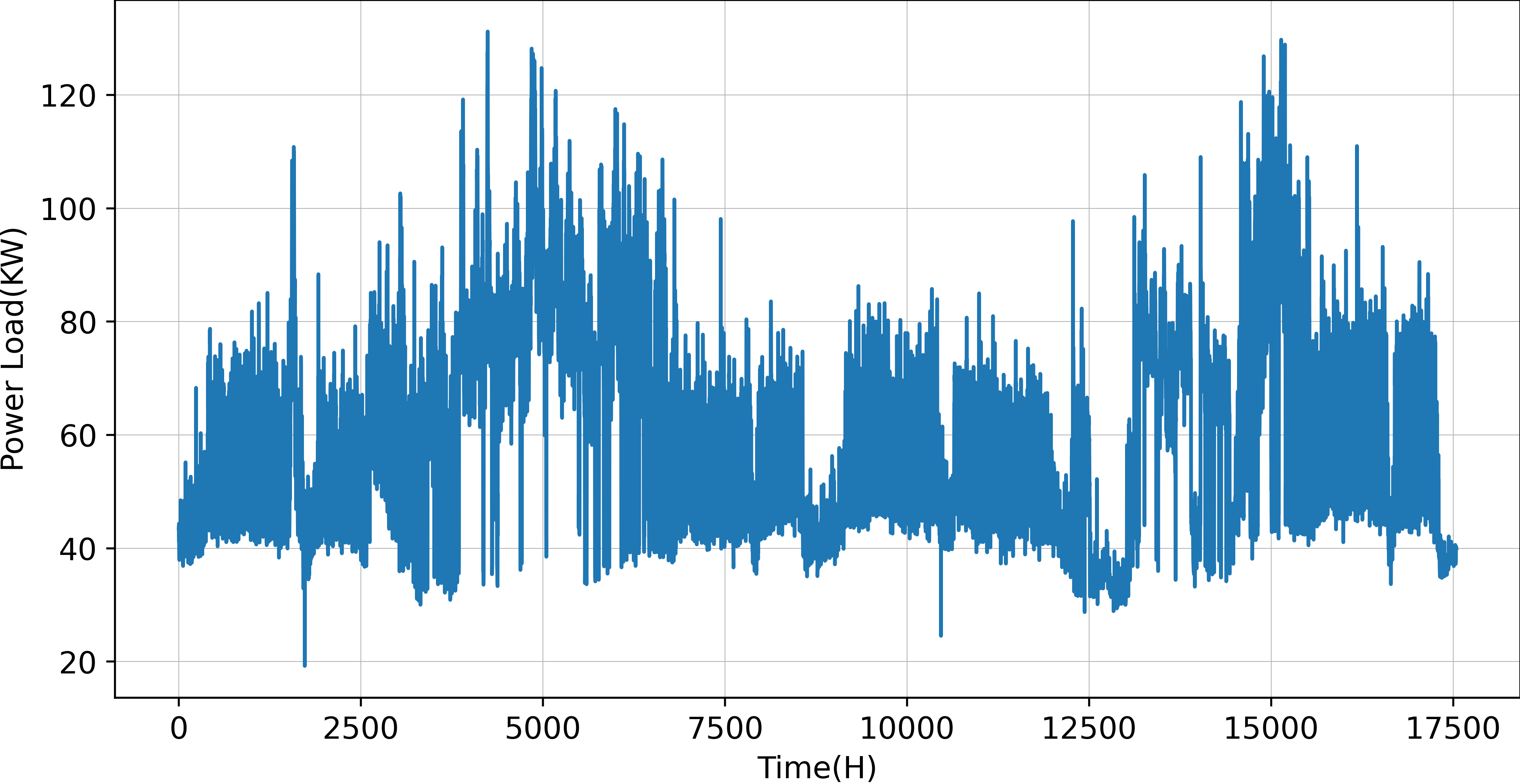
Figure 6: One of the building data sets contains many outliers.

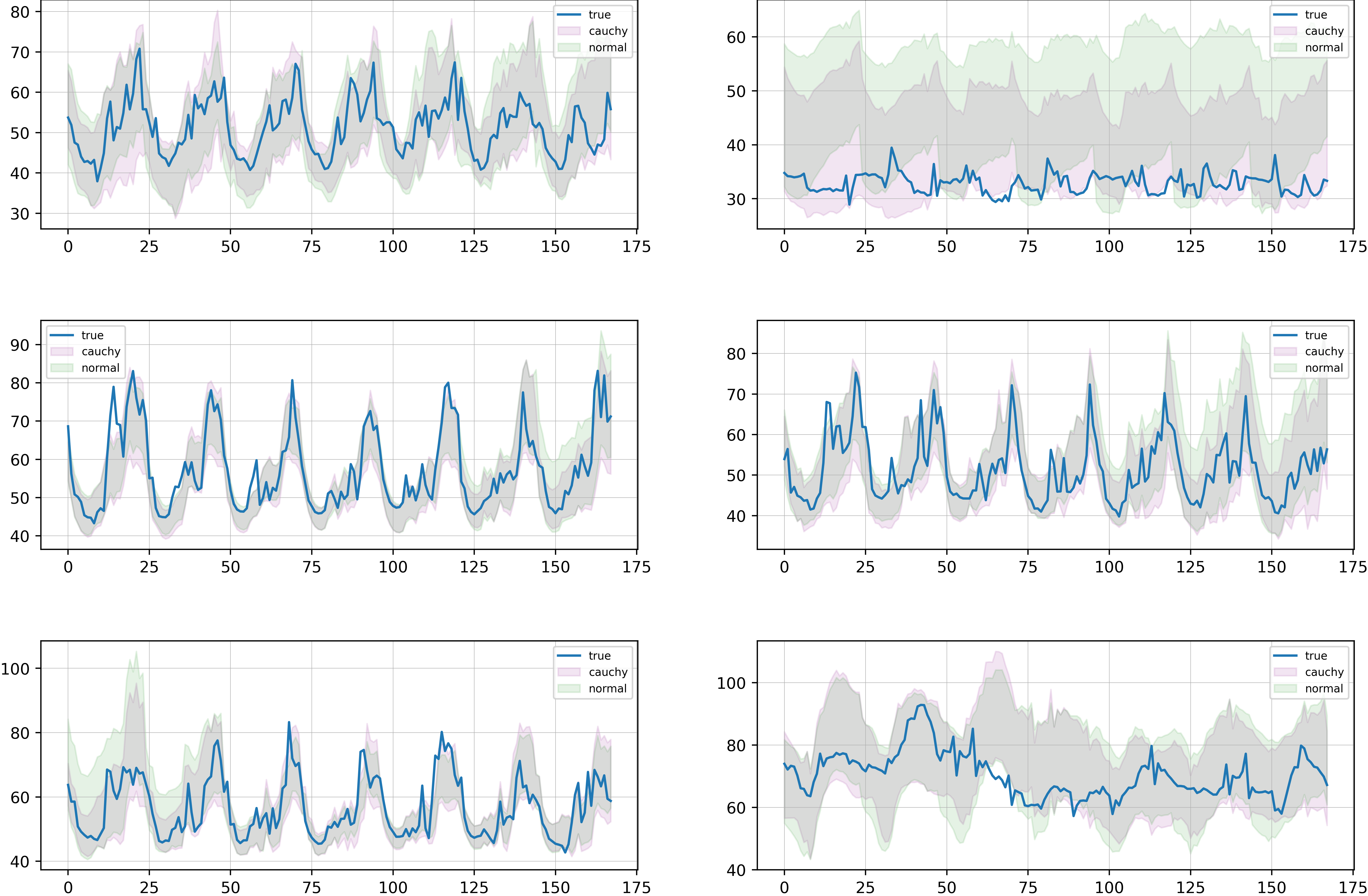
Figure 7: Visualization of comparison between Gaussian and Cauchy

Table 8: Ablation study

Dataset	Metric	o/o	d/o	d/c
GEF	MAPE	3.58	3.44	3.29
COV		2.04	2.13	1.91
BDG2		12.46	11.95	10.83
GEF	MAE	119.47	115.37	110.44
COV		21844.0	22512.37	20308.3
BDG2		12.76	12.38	11.18
GEF	Winker Score(25%)	75.88	73.39	70.69
COV		13966.92	14398.77	13063.04
BDG2		8.14	7.93	7.17
GEF	Winker Score(50%)	96.66	93.22	90.94
COV		18069.34	18601.00	17112.44
BDG2		10.48	10.28	9.36
GEF	Winker Score(75%)	131.00	124.18	121.03
COV		25408.52	25988.62	23399.30
BDG2		14.39	14.26	13.60
GEF	CRPS	86.61	83.07	83.24
COV		16263.42	16705.65	15435.79
BDG2		9.35	9.16	8.72

• o/o: without diffusion structure and use the Normal distribution.

• d/o: with diffusion structure and use the Normal distribution.

• d/c: with diffusion structure and use the Cauchy distribution.

3.3.4 Time Consuming Comparison

Although uncertainty estimation based on methods such as ensemble and Bayesian neural networks can improve forecasting accuracy (compared to simple DeepAR), the additional computational costs cannot be ignored. Figure 8 shows the time required for one training on ten building datasets. Because the deep ensemble approach necessitates training numerous separate neural networks, its training time increases linearly when compared to standard DeepAR. Similarly, the Bayesian neural network technique treats every parameter of the neural network as a random variable with a minimum order of magnitude of a million. Therefore, it is no wonder that these methods require much more computational resources than other methods. The dropout approach is less computationally intensive than other uncertainty estimating techniques, but it might result in inconsistent training and inference processes, which can quickly reduce forecasting accuracy li2019understanding (also shown in the poor performance in the COV dataset). When compared to the Bayesian and Ensemble approaches, our method does not significantly differ from the simple model, even though it takes more computing time than the simple deep AR model because of the addition of diffusion structures.

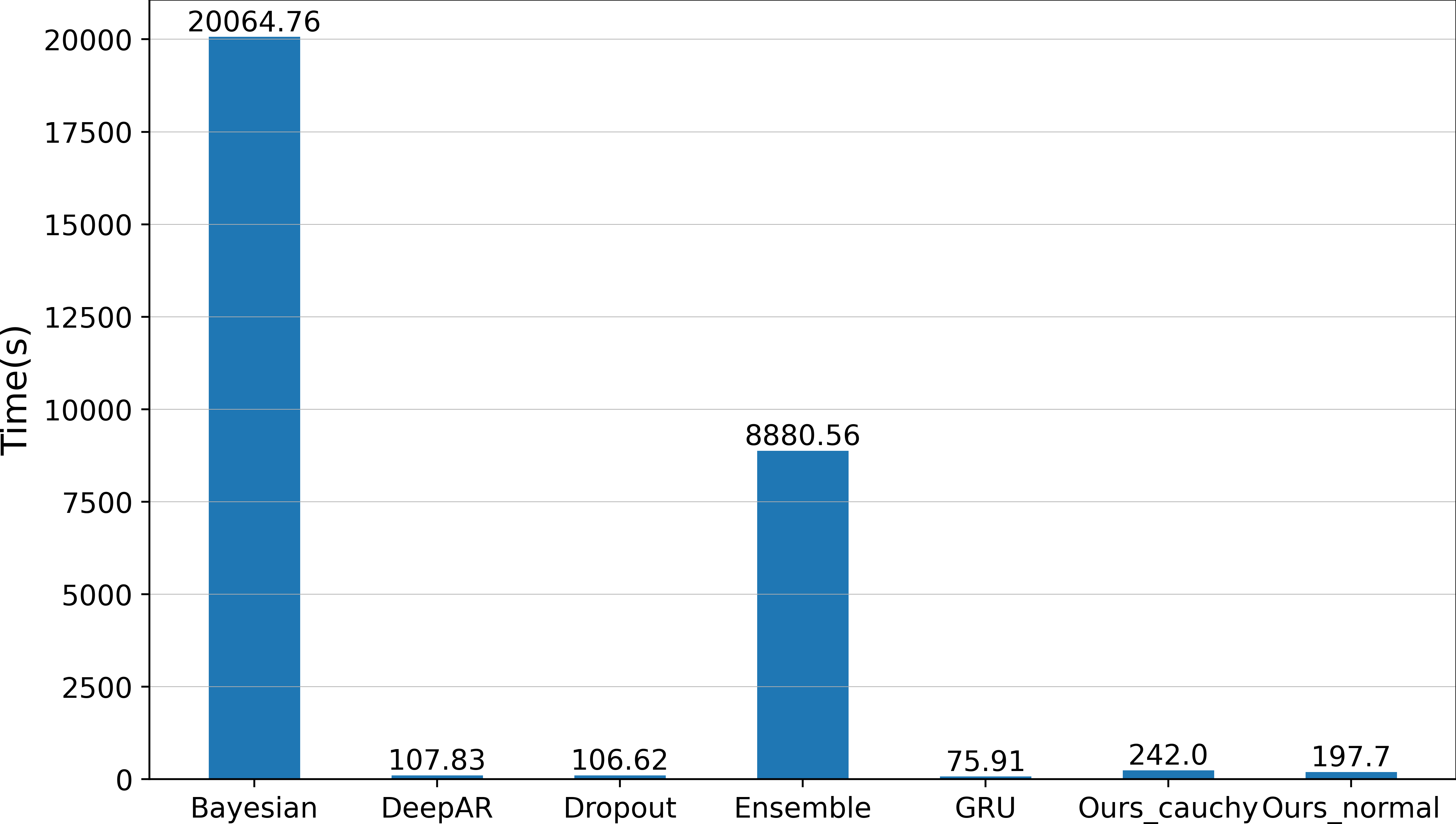
Figure 8: Time consumed by different methods.

4 Conclusions

In this paper, we propose a novel method for estimating uncertainty and apply it to load forecasting. On one hand, we employ a robust heavy-tailed Cauchy distribution to encapsulate our forecasting model, reducing the model’s sensitivity to outliers and sudden changes. This approach ensures the model’s training stability while estimating aleatoric uncertainty. On the other hand, we propose a novel empirical estimation method based on the diffusion model. Unlike traditional methods that focus on the model’s parameters, our approach utilizes the hidden state in Seq2seq to estimate uncertainty, significantly reducing the training time and providing superior probabilistic forecasts. In future work, we will consider combining this estimation method with online learning to achieve higher forecasting accuracy through adaptive model updates based on uncertainty estimation.

References

- (1) T. Hong, et al., Energy forecasting: Past, present, and future, Foresight: The International Journal of Applied Forecasting (32) (2014) 43–48.
- (2) M. A. Hammad, B. Jereb, B. Rosi, D. Dragan, et al., Methods and models for electric load forecasting: a comprehensive review, Logist. Sustain. Transp 11 (1) (2020) 51–76.
- (3) Z. Zhu, W. Chen, R. Xia, T. Zhou, P. Niu, B. Peng, W. Wang, H. Liu, Z. Ma, X. Gu, J. Wang, Q. Chen, L. Yang, Q. Wen, L. Sun, Energy forecasting with robust, flexible, and explainable machine learning algorithms, AI Magazine (2023).
- (4) N. Huang, S. Wang, R. Wang, G. Cai, Y. Liu, Q. Dai, Gated spatial-temporal graph neural network based short-term load forecasting for wide-area multiple buses, International Journal of Electrical Power & Energy Systems 145 (2023) 108651.
- (5) A. Vaghefi, M. A. Jafari, E. Bisse, Y. Lu, J. Brouwer, Modeling and forecasting of cooling and electricity load demand, Applied Energy 136 (2014) 186–196.
- (6) K. B. Lindberg, S. J. Bakker, I. Sartori, Modelling electric and heat load profiles of non-residential buildings for use in long-term aggregate load forecasts, Utilities Policy 58 (2019) 63–88.
- (7) Y. Wang, S. Sun, X. Chen, X. Zeng, Y. Kong, J. Chen, Y. Guo, T. Wang, Short-term load forecasting of industrial customers based on svmd and xgboost, International Journal of Electrical Power & Energy Systems 129 (2021) 106830.
- (8) A. Almalaq, G. Edwards, A review of deep learning methods applied on load forecasting, in: 2017 16th IEEE international conference on machine learning and applications (ICMLA), 2017, pp. 511–516.
- (9) Y. Zhou, Z. Ding, Q. Wen, Y. Wang, Robust load forecasting towards adversarial attacks via bayesian learning, IEEE Transactions on Power Systems 38 (2) (2023) 1445–1459.
- (10) M. Grabner, Y. Wang, Q. Wen, B. Blažič, V. Štruc, A global modeling framework for load forecasting in distribution networks, IEEE Transactions on Smart Grid (2023).
- (11) W. Kong, Z. Y. Dong, Y. Jia, D. J. Hill, Y. Xu, Y. Zhang, Short-term residential load forecasting based on lstm recurrent neural network, IEEE transactions on smart grid 10 (1) (2017) 841–851.
- (12) A. Li, F. Xiao, C. Zhang, C. Fan, Attention-based interpretable neural network for building cooling load prediction, Applied Energy 299 (2021) 117238.
- (13) R. Jiao, S. Wang, T. Zhang, H. Lu, H. He, B. B. Gupta, Adaptive feature selection and construction for day-ahead load forecasting use deep learning method, IEEE Transactions on Network and Service Management 18 (4) (2021) 4019–4029.
- (14) A. G. Journel, Modeling uncertainty: some conceptual thoughts, in: Geostatistics for the Next Century: An International Forum in Honour of Michel David’s Contribution to Geostatistics, Montreal, 1993, Springer, 1994, pp. 30–43.
- (15) Y. Wang, D. Gan, M. Sun, N. Zhang, Z. Lu, C. Kang, Probabilistic individual load forecasting using pinball loss guided lstm, Applied Energy 235 (2019) 10–20.
- (16) L. Xu, S. Wang, R. Tang, Probabilistic load forecasting for buildings considering weather forecasting uncertainty and uncertain peak load, Applied energy 237 (2019) 180–195.
- (17) K. Rasul, C. Seward, I. Schuster, R. Vollgraf, Autoregressive denoising diffusion models for multivariate probabilistic time series forecasting, in: International Conference on Machine Learning, PMLR, 2021, pp. 8857–8868.
- (18) L. Shen, J. Kwok, Non-autoregressive conditional diffusion models for time series prediction, arXiv preprint arXiv:2306.05043 (2023).
- (19) A. Kendall, Y. Gal, What uncertainties do we need in bayesian deep learning for computer vision?, Advances in neural information processing systems 30 (2017).
- (20) Y. Yang, W. Li, T. A. Gulliver, S. Li, Bayesian deep learning-based probabilistic load forecasting in smart grids, IEEE Transactions on Industrial Informatics 16 (7) (2019) 4703–4713.
- (21) M. Sun, T. Zhang, Y. Wang, G. Strbac, C. Kang, Using bayesian deep learning to capture uncertainty for residential net load forecasting, IEEE Transactions on Power Systems 35 (1) (2019) 188–201.
- (22) Y. Gal, Z. Ghahramani, Dropout as a bayesian approximation: Representing model uncertainty in deep learning, in: international conference on machine learning, PMLR, 2016, pp. 1050–1059.
- (23) B. Lakshminarayanan, A. Pritzel, C. Blundell, Simple and scalable predictive uncertainty estimation using deep ensembles, Advances in neural information processing systems 30 (2017).
- (24) P. J. Huber, Robust statistics, in: International encyclopedia of statistical science, Springer, 2011, pp. 1248–1251.
- (25) X. Li, S. Chen, X. Hu, J. Yang, Understanding the disharmony between dropout and batch normalization by variance shift, in: Proceedings of the IEEE/CVF conference on computer vision and pattern recognition, 2019, pp. 2682–2690.
- (26) B. Dai, D. Wipf, Diagnosing and enhancing vae models, arXiv preprint arXiv:1903.05789 (2019).
- (27) G. Papamakarios, E. Nalisnick, D. J. Rezende, S. Mohamed, B. Lakshminarayanan, Normalizing flows for probabilistic modeling and inference, The Journal of Machine Learning Research 22 (1) (2021) 2617–2680.
- (28) J. Ho, A. Jain, P. Abbeel, Denoising diffusion probabilistic models, Advances in Neural Information Processing Systems 33 (2020) 6840–6851.
- (29) D. M. Blei, A. Kucukelbir, J. D. McAuliffe, Variational inference: A review for statisticians, Journal of the American statistical Association 112 (518) (2017) 859–877.
- (30) E. Nachmani, R. S. Roman, L. Wolf, Denoising diffusion gamma models, arXiv preprint arXiv:2110.05948 (2021).
- (31) L. Li, J. Yan, Q. Wen, Y. Jin, X. Yang, Learning robust deep state space for unsupervised anomaly detection in contaminated time-series, IEEE Transactions on Knowledge and Data Engineering (2022).
- (32) J. Gao, X. Song, Q. Wen, P. Wang, L. Sun, H. Xu, RobustTAD: Robust time series anomaly detection via decomposition and convolutional neural networks, KDD Workshop on Mining and Learning from Time Series (KDD-MileTS’20) (2020).
- (33) P. G. Georgiou, P. Tsakalides, C. Kyriakakis, Alpha-stable modeling of noise and robust time-delay estimation in the presence of impulsive noise, IEEE transactions on multimedia 1 (3) (1999) 291–301.
- (34) D. Salinas, V. Flunkert, J. Gasthaus, T. Januschowski, Deepar: Probabilistic forecasting with autoregressive recurrent networks, International Journal of Forecasting 36 (3) (2020) 1181–1191.
- (35) T. Hong, P. Pinson, S. Fan, H. Zareipour, A. Troccoli, R. J. Hyndman, Probabilistic energy forecasting: Global energy forecasting competition 2014 and beyond (2016).
- (36) C. Miller, A. Kathirgamanathan, B. Picchetti, P. Arjunan, J. Y. Park, Z. Nagy, P. Raftery, B. W. Hobson, Z. Shi, F. Meggers, The building data genome project 2, energy meter data from the ashrae great energy predictor iii competition, Scientific data 7 (1) (2020) 368.
- (37) M. Farrokhabadi, J. Browell, Y. Wang, S. Makonin, W. Su, H. Zareipour, Day-ahead electricity demand forecasting competition: Post-covid paradigm, IEEE Open Access Journal of Power and Energy 9 (2022) 185–191.
- (38) J. E. Matheson, R. L. Winkler, Scoring rules for continuous probability distributions, Management science 22 (10) (1976) 1087–1096.
- (39) C. Wang, D. Qin, Q. Wen, T. Zhou, L. Sun, Y. Wang, Adaptive probabilistic load forecasting for individual buildings, iEnergy 1 (3) (2022) 341–350.
- (40) K. Cho, B. Van Merriënboer, C. Gulcehre, D. Bahdanau, F. Bougares, H. Schwenk, Y. Bengio, Learning phrase representations using rnn encoder-decoder for statistical machine translation, arXiv preprint arXiv:1406.1078 (2014).
- (41) D. Tran, M. Dusenberry, M. Van Der Wilk, D. Hafner, Bayesian layers: A module for neural network uncertainty, Advances in neural information processing systems 32 (2019).
- (42) J. Postels, F. Ferroni, H. Coskun, N. Navab, F. Tombari, Sampling-free epistemic uncertainty estimation using approximated variance propagation, in: Proceedings of the IEEE/CVF International Conference on Computer Vision, 2019, pp. 2931–2940.