The Chaotic Milling Behaviors of Interacting Swarms After Collision

Abstract

We consider the problem of characterizing the dynamics of interacting swarms after they collide and form a stationary center of mass. Modeling efforts have shown that the collision of near head-on interacting swarms can produce a variety of post-collision dynamics including coherent milling, coherent flocking, and scattering behaviors. In particular, recent analysis of the transient dynamics of two colliding swarms has revealed the existence of a critical transition whereby the collision results in a combined milling state about a stationary center of mass. In the present work we show that the collision dynamics of two swarms that form a milling state transitions from periodic to chaotic motion as a function of the repulsive force strength and its length scale. We used two existing methods as well as one new technique: Karhunen-Loeve decomposition to show the effective modal dimension chaos lives in, the 0-1 test to identify chaos, and then Constrained Correlation Embedding to show how each swarm is embedded in the other when both swarms combine to form a single milling state after collision. We expect our analysis to impact new swarm experiments which examine the interaction of multiple swarms.

Swarms, which consist of agents with simple rules, are ubiquitous in nature and exhibit many different types of emergent dynamical behavior. Much recent work has explored the dynamics of single swarm that depend on general physical parameters, such as attraction, repulsion, alignment and communication delay. The collective patterns have been derived from bifurcation theory and mean-field analyses. However, much less is known about the dynamical behavior of multiple interacting and colliding swarms. Colliding swarms have been found to have collective behaviors, such as milling, flocking and scattering states. Milling, in particular, is created when one swarm captures another resulting in a stationary center of mass. Applying existing methods of analyzing the dynamics of colliding swarms, we describe the long term dynamics of the captured milling states. Specifically, we show the resulting dynamics starts from periodic behavior, going through quasi-periodic behavior on a torus, which then leads to chaotic behavior as a function of repulsive strength.

I Introduction

Improved data gathering and analysis techniques have enabled researchers to collect data and analyze the motions of individual agents in biological flocks, and formulate more accurate, empirical models for collective motion strategies of flocking species such as birds, fish and insects, Li and Sayed (2012); Theraulaz et al. (2002). The derived mechanics has resulted in the translation of swarm theory to communicating robotic systems. Swarms of collaborating robots have been proposed for conducting tasks including search and rescue, density control, and mapping Li et al. (2017); Ramachandran, Elamvazhuthi, and Berman (2018).

From general models of swarm dynamics, one observes three basic swarming states or modes: flocking, in which a center of mass moves in a straight line with a constant velocity; milling, where the agents rotate coherently around a stationary center of mass; and rotating, where the center of mass itself rotates about a fixed point in space Szwaykowska, Schwartz, and Carr (2018); Edwards et al. (2020); Hindes et al. (2021). Much is known about the behaviors and stability of single swarms with physics-informed, nonlinear interactions Levine, Rappel, and Cohen (2000); Minguzzi (2015); D’Orsogna et al. (2006); y Teran-Romero, Forgoston, and Schwartz (2012). They are able to converge to organized, coherent behaviors in spite of complicating factors such as communication delay, localized number of neighbors each agent is able to interact with, a consensus force, heterogeneity in agent dynamics, and environmental noise Ling et al. (2019); Mier-y Teran-Romero, Forgoston, and Schwartz (2011); Szwaykowska et al. (2016); Schwartz et al. (2020). However, in many applications, beyond the dynamics of single swarms, multiple swarms interact and produce even more complex spatio-temporal behaviors.

New studies have begun to address swarm-on-swarm dynamics, and in particular the scattering of two large, colliding swarms with nonlinear interactions. Recent numerical studies have shown that when two flocking swarms collide, the resulting dynamics typically appear as a merging of the swarms into a single flock, milling as one uniform swarm, or scattering into separate composite flocks moving in different directions Armbruster, Martin, and Thatcher (2017); Kolon and Schwartz (2018); Sartoretti and Hongler (2016). However, more detailed analytical understanding of how and when these behaviors occur is necessary, especially when designing robotic swarm experiments such as swarm herding and capture Chipade and Panagou (2019, 2020); Park et al. (2018) and controlling their outcomes.

Building on early numerical insights, it has been shown that one can predict the critical swarm-on-swarm interaction coupling, below which two colliding swarms merely scatter, as a function of a physical swarm parameter Hindes et al. (2021). In particular, analysis of the transient dynamics of two colliding swarms, seen in Fig. 1, has revealed the existence of a critical transition whereby the collision results in a combined milling state, where one swarm is embedded in the other. However, what is missing is a quantitative description of the post-collision asymptotic dynamics.

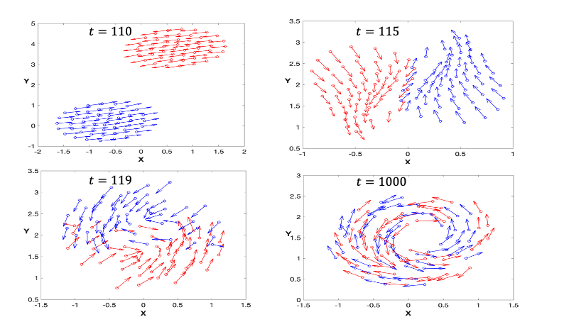
Figure 1: Four time-snapshots for different values of t, showing each swarm with different colors: red and blue circles. Velocities are drawn with arrows. Swarm parameters are: C = 1.15, N = 50.

In the current work, our starting point is Fig. 2. We observe that after the colliding swarms have settled down to a milling behaviors, the dynamics change from periodic to quasi-periodic, and to chaotic motions for different values of repulsion strength. We examine the dimensionality of the combined mill by computing its Karhunen-Loeve dimension. It is a measure of the variance of the entire post-collision attractor, and computes how many expansion modes it takes to capture the dynamics. Next, we aim to numerically confirm that the two swarms near collisions displayed complex chaotic behavior with two methods. First, we determine whether the collision dynamics is chaotic, by using the existing binary test for chaos. Finally, we defined the constrained correlation embedding to quantify the dynamical complexity of the combined milling state.

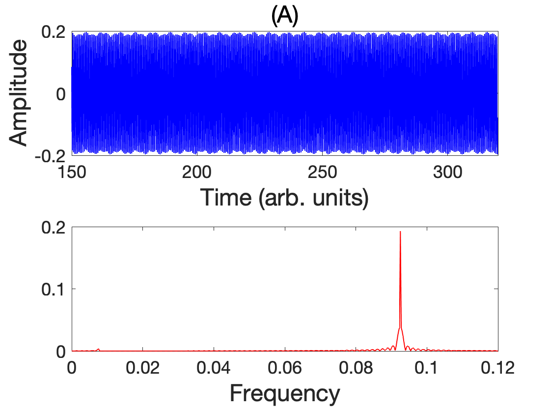
Figure 2: Dimensionless time-series (top) and frequency (bottom) of y component of a single agent randomly chosen, for (A): C = 0.51, (B): C = 0.70 and (C):C = 0.89. Accordingly, we have observed periodicity (A), a motion on torus (B) and chaos (C).

II Swarm Model

To make progress, we considered a class of well-known deterministic swarming models for both discrete Albi et al. (2014); Bernoff and Topaz (2011); Levine, Rappel, and Cohen (2000) and continuous Bernoff and Topaz (2011); Minguzzi (2015) systems consisting of mobile agents moving under the influence of self-propulsion, nonlinear damping, and pairwise interaction forces. In the absence of interactions, each swarmer tends to a fixed speed, which balances its self-propulsion and damping, that is translationally invariant Hindes et al. (2020). A simple model that captures the basic physics is

$$\ddot{\mathbb{r}}_{i}=\big{[}\alpha-\beta|\dot{\mathbb{r}}_{i}|^{2}\big{]}\dot{\mathbb{r}}_{i}-\lambda\sum_{j\neq i}\partial_{\mathbb{r}_{i}}U(|\mathbb{r}_{j}-\mathbb{r}_{i}|)$$ (1)

where $\mathbb{r}_{i}$ is the position-vector for the $i$th agent in two spatial dimensions, $\alpha$ is a self-propulsion constant, $\beta$ is a nonlinear damping constant, and $\lambda$ is a coupling constant Levine, Rappel, and Cohen (2000); Minguzzi (2015); D’Orsogna et al. (2006); y Teran-Romero, Forgoston, and Schwartz (2012). The total number of swarming agents is $N$, and each agent has unit mass. Beyond providing a basis for theoretical insights, Eq.(1) has been implemented in mixed-reality experiments with several robotics platforms including autonomous ground, surface, and aerial vehiclesChuang et al. (2007); Szwaykowska et al. (2016).

An example interaction potential that we consider in detail is the Morse potential,

$$U(r)=Ce^{-r/l}-e^{-r}.$$ (2)

This is a common model for implicit interactions with local repulsion and attraction length scales, scaled as $l$ and $1$, respectivelyD’Orsogna et al. (2006); Bernoff and Topaz (2011). In the following, we assume that two interacting swarms are subject to the same underlying physics, Eqs.(1-2), but with different initial conditions. Each swarm will be initially separated by a large distance compared to the interaction length scales, $l$ and $1$. Therefore, the interaction force an agent feels will be at early times effectively confined to their own swarm, given the exponential decay with distance implied by Eq.(2).

For the swarm flocks that are nearly aligned upon collision, the relevant initial-condition parameter is the distance between the two flocks as they approach $x\!=\!0$, regardless of the direction of their velocities. This distance is often called the impact parameter, $\Delta y$, in classical mechanicsLandau and Lifshitz (1976), and it represents the closest distance the two flocks would approach in the absence of interaction forces. Depending on the value of impact parameter and the coupling strength after collision, the two flocks typically translate as one, scatter or form a combined mill.

Based on the previous numerical experiments for different values of $\Delta y$ and $\lambda$ Hindes et al. (2021), we are particularly interested in collisions that result in a swarm milling state. Representative parameters for generating milling states upon collision are: $l=0.5,\alpha=1.0,\beta=5.0,\lambda=0.1,\Delta y=4.0$, which are assumed throughout this work. See Hindes et al. (2021) for further details. Our aim is to vary the repulsive strength and observe the changes in the dynamic behaviors of milling after the collision. Having noticed that changing repulsion drastically changes the post-collision dynamics, we then turned our attention to quantify the complexity of the dynamics so that we can try to deduce the dynamic consequences as we sweep parameters. One useful technique is Karhunen-Loeve decomposition, which we address next.

III Dimensionality Analysis: Karhunen-Loeve decomposition of swarms of N-agents

Karhunen-Loeve (KL) decomposition is a procedure of mode expansion for spatio-temporal processes that extracts the relevant degrees of freedom of the dynamics of a large data set. We measured the number of Karhunen-Loeve(KL) modes needed to capture most of the the dynamic variance. It is an effective way to learn model reduction while describing the space in which the asymptotic dynamics resides. Known as the method of snapshots Sirovich (1987), KL analysis correlates dynamics in time while averaging in space. Note that KL mode decomposition essentially is Principle Component Analysis in the time domain Jolliffe and Cadima (2016). In order to identify correlations, we compute the covariance matrix, where each entry is correlation of two snapshots. The modes are defined by the data and constitute a natural coordinate system that approximates from time-series data optimally in space with the $L_{2}$ norm. From Eq. 1, assume we have $N$ agents, which are sampled at $M$ time points. Since both positions and velocities are changing with time, we define the sequence of data snapshots to include both position and velocity by letting

$$\mathbb{z}(t_{j})=[\mathbb{r}_{1}(t_{j}),...,\mathbb{r}_{N}(t_{j});\mathbb{v}_{1}(t_{j}),...,\mathbb{v}_{N}(t_{j})].$$ (3)

where $j\in\{1,2,...,M\}$ Rao and Ahmed (1976). We assume the field can be expanded in a split time-space sum of modes given by

$$\mathbb{z}(t_{j})=\sum_{i=1}^{M}{\alpha}_{i}(t_{j})\bm{\phi}_{i}=\mathcal{A}_{j,i}\bm{\phi}_{i}.$$ (4)

The matrix $\mathcal{A}_{j,i}$ stores the elements of the amplitudes at time $t_{j}$ as rows. That is, each row of the array is one mode. The vectors $\bm{\phi}_{i}$ are of the same dimension as of $\mathbb{z}(t_{i})$ filed at a given snapshot. We define the residual using $M$ modes over time as

$$\mathcal{E}=\lVert\mathbb{z}(t_{j})-\sum_{i=1}^{M}{\alpha}_{i}(t_{j})\bm{\phi}_{i}\rVert_{L_{2}},\;j\in\{1,2,...M\}.$$ (5)

Minimizing $\mathcal{E}$ generates an eigenvalue problem for the first temporal mode; i.e., we solve

$$\mathcal{C}\bm{\alpha}_{i}=\lambda_{i}\bm{\alpha}_{i},$$ (6)

where $\mathcal{C}$ is an $M\times M$ covariance matrix. The $ij^{th}$ element is given by

$$[\mathcal{C}]_{ij}=\frac{<\mathbb{z}(t_{i}),\mathbb{z}(t_{j})>}{N},$$ (7)

$<>$ denotes an inner product. Since the covariance matrix is symmetric, the eigenvalues are real, non-negative. Then we have ordering such that

$$\lambda_{1}\geq\lambda_{2}\geq...\geq\lambda_{M}\geq 0.$$ (8)

The corresponding eigenvectors, $\bm{\alpha}_{i}$, are the temporal modes.
To find the spatial modes, we make use of the fact that the modes from $\mathcal{C}$ are orthonormal;

$$\sum_{j=1}^{M}{\alpha}_{l}(t_{j}){\alpha}_{m}(t_{j})=\delta_{lm}.$$ (9)

Finally, we have

$$\sum_{i=1}^{M}\mathbb{z}(t_{j}){\alpha}_{i}(t_{j})=\sum_{j=1}^{M}\sum_{i=1}^{M}{\alpha}_{i}(t_{j}){\alpha}_{k}(t_{j})\bm{\phi}_{i}=\bm{\phi}_{k}.$$ (10)

We may now approximate the original spatial-temporal field by examining the total variance, which may be computed from the eigenvalues. Let

$$\Lambda=\sum\lambda_{i},$$ (11)

and normalize the eigenvalues by setting

$$\bar{\lambda_{i}}=\frac{\lambda_{i}}{\Lambda},i=1,2,...M.$$ (12)

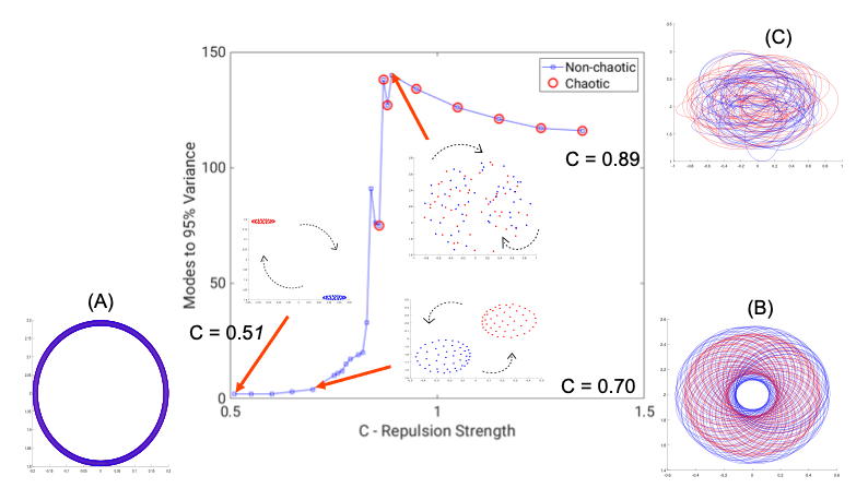
Figure 3: The 0-1 chaos test result (red circles) plotted over KL mode decomposition (blue circles). The x axis represents values of repulsive strength, C, and y axis is the number of KL modes needed to capture 95 percent of the total variance. The figures outside of the graph axis, (A)-(C), are the multi-agent attractor time series projected onto the x-y plane corresponding to the time-series in Fig. 2. The figures inside the axes are the corresponding fixed time snapshots showing the individual agents. This is to show that in real time, combined milling of two swarms are fragmented while it is not clear from the multi-agent attractor time-series projected onto the x-y plane.

We examine the cumulative sum of $\bar{\lambda_{i}}$ so that the total variance exceeds a threshold, $T.$ Here $T$ is arbitrarily chosen to be 95 percent. After transients are removed, in order to capture 95 percent of the full data, for instance, Fig. 3 indicates that 4 KL modes are needed for C= 0.51, 6 modes for C = 0.70 and about 140 modes for C = 0.89. In other words, one can see that when the post collision dynamics is periodic, it only requires four modes to describe the effective limit cycle behavior. As the repulsion strength is increased, the dynamics lies on a torus, which may be thought of as two coupled oscillators. However, the torus then breaks up, as the repulsion is further increased and the resulting transition is to a chaotic behavior, corresponding to a substantial change in KL dimension, from 4 to 140. The rapid change in KL dimension signals a dramatic transition in dynamical complexity. As we increase the repulsion strength, the combined milling behavior becomes qualitatively more complex exponentially from collective oscillations. Since the dynamics becomes quite complex and seemingly chaotic, we next turn to formally extracting whether or not is is technically chaotic for large repulsion.

IV Binary Test for Chaos: 0 - 1 Test

For its ease of use and vast applicability, we employed the 0-1 test Gottwald and Melbourne (2004, 2009a) to distinguish chaotic and non-chaotic parameter regions in our systems. We input one-dimensional time series $\phi(n),n\leq\bar{N}\in\mathbb{N}$ where $\bar{N}$ denotes the number of data points used. and it produces two-dimensional Euclidean extension $P(n)$ and $Q(n)$. The main idea is to assess whether the trajectories of the systems are bounded. Let $\phi(n)$ be an observed time-series of the underlying system. Gottwald and Melbourne (2004) . For an arbitrary $a>0$ that is randomly chosen, usually from $(0,\pi)$, we define $P(n)$ and $Q(n)$ for each $a$ as

$$P_{a}(n)=\sum_{j=1}^{n}\phi(n)\cos(ja),\;\;Q_{a}(n)=\sum_{j=1}^{n}\phi(n)\sin(ja).$$ (13)

Figure 4: P vs Q plot obtained for (A): C = 0.51, (B): C = 0.70 and (C): C = 0.89. P and Q are obtained in the process of 0 -1 test. Underling system is regular if the PQ plot is bounded, and it is said to be chaotic if it is diffusive.

We then compute the mean square displacement defined by

$$\begin{split}M_{a}(n)=&\lim_{\bar{N}\to\infty}\frac{1}{\bar{N}}\sum_{j=1}^{\bar{N}}([P_{a}(j+n)-P_{a}(j)]^{2}\\ +&[Q_{a}(j+n)-Q_{a}(j)]^{2})],\end{split}$$ (14)

requiring $\bar{N}\gg n$. The limit is guaranteed by calculating Eq.14 only for $n\leq n_{\text{cut}}$ where $\bar{N}\gg n_{\text{cut}}$, and $n_{\text{cut}}=\frac{\bar{N}}{10}$Gottwald and Melbourne (2009a). The test for chaos is based on the growth rate of the mean square displacement as a function of $n$. We calculated the asymptotic growth rate of Eq.14 defined as

$$K_{a}=\lim_{\bar{N}\to\infty}\frac{log(M_{a}(n))}{log(n)}.$$ (15)

Eq.14 is bounded if $\phi(n)$ is regular, or it grows linearly in time if $\phi(n)$ is chaotic Gottwald and Melbourne (2009b). Therefore, the 0-1 test states that a value of $K\approx 0$ indicates regular dynamics, and $K\approx 1$ indicates chaotic dynamics. For continuous systems such as differential equations, one might encounter an inaccurate test result due to oversampling Melbourne and Gottwald (2007); Gottwald and Melbourne (2009a). We address this issue by incorporating two routine checks suggested in Matthews . If the underlying dynamical system is regular, then its PQ plot is bounded; it is chaotic if the plot is diffusive. Figure  4 identifies with the dynamics observation from the time-series in Fig. 2. Note that the 0 -1 test only distinguishes chaos from regular dynamics, and is unable to detect quasi- periodicity.

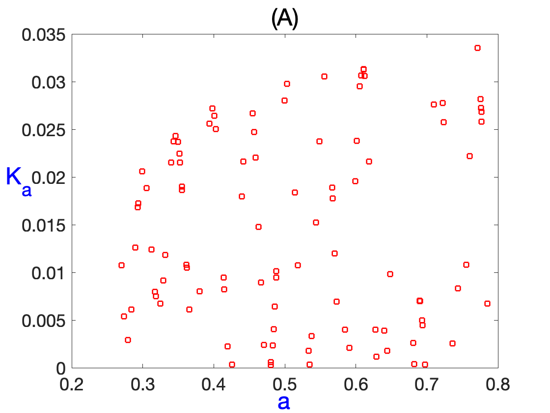
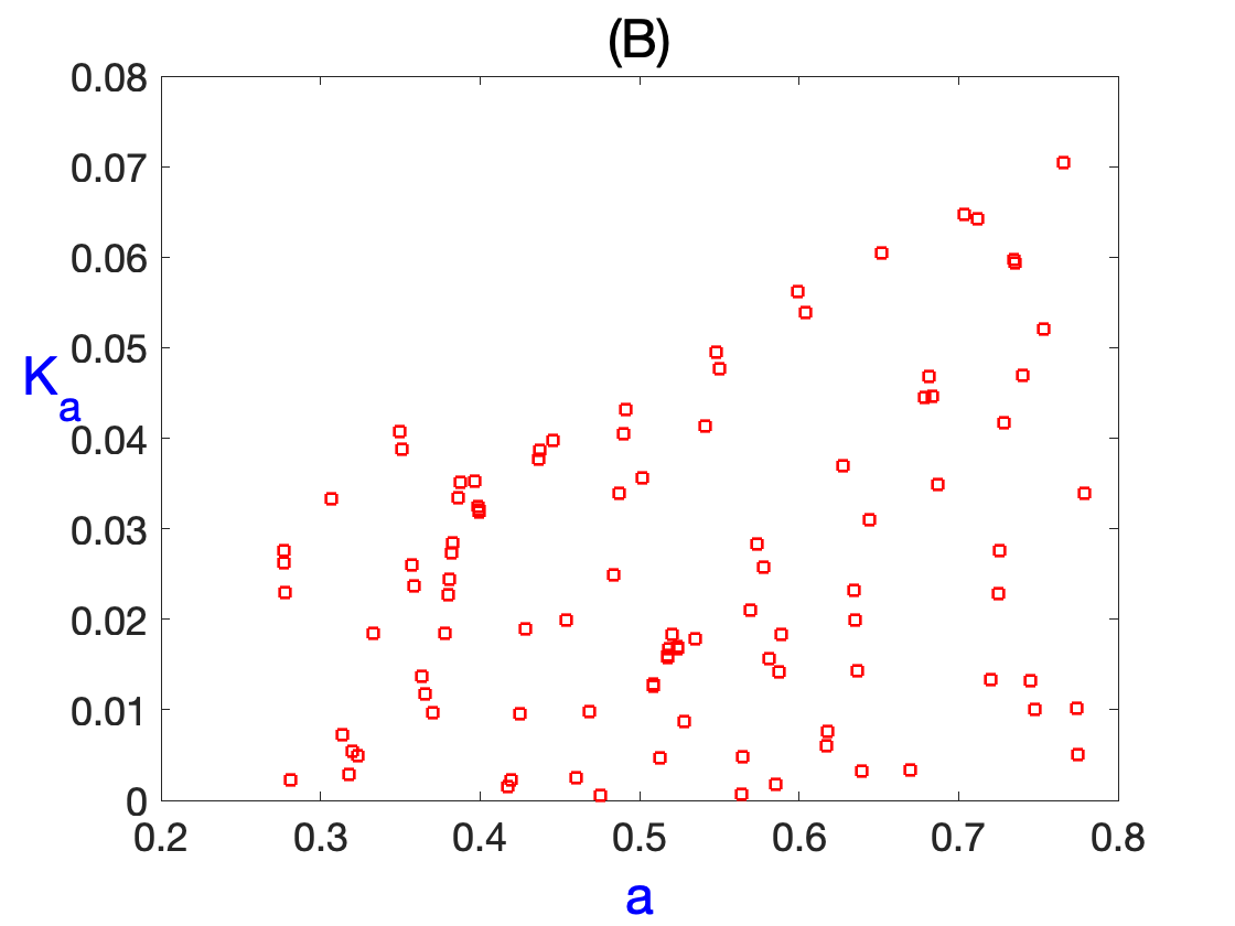
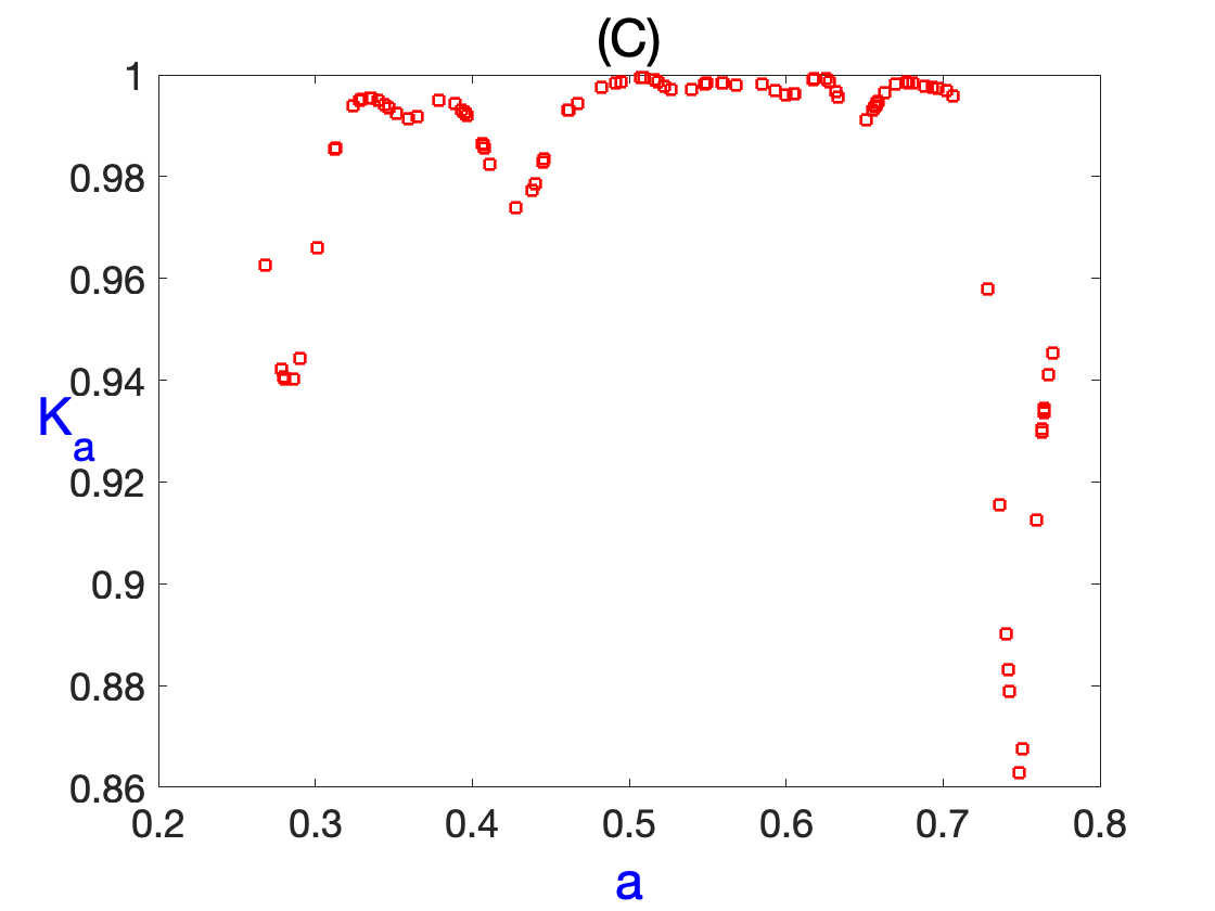
Figure 5: 0 -1 test plots for (A):C = 0.51, (B):C = 0.70 and (C):C = 0.89. The result was computed for 100 randomly selected values of $a\in[\frac{\pi}{10},\frac{2\pi}{10}]$ against corresponding value of $K_{a}$ for each such $a$.

In our implementation of the 0 - 1 test, we used 100 data points, i.e., $N_{a}=100,$ from the time-series of y component of a randomly chosen agent. It was collected from a post-collision milling state for various of repulsive strength $C$ Hindes et al. (2021), excluding the transients. We then calculated $K_{a}$ for each $a$ randomly chosen from $[\frac{\pi}{10},\frac{2\pi}{10}]$ in accordance with an observation described in Gottwald and Melbourne (2008) to avoid oversampling (Fig. 5). The indicator for chaotic behaviors, denoted as $K$, of our system for a given repulsive strength is then $K=$ median$(K_{a})$. We computed such $K$ as a function of varying repulsive strength $C$.

Figure  6 shows that the dynamics is regular for the repulsive strength $C$ that are in the range of 0.50 to 0. 81-83. As the value of $C$ increases, the value of $K$ starts to tend to 1, indicating chaos from onward around $C=0.84$. This roughly corresponds to the increasing trend of number of modes predicted by the KL decomposition depicted in Fig. 3. However, the 0-1 test does not provide any information about the specific properties or behaviors of the system beyond its chaotic or non-chaotic nature. It cannot tell us anything about the attractors, periodic orbits, bifurcations, or other features that may be present in the system such as quasi periodicity. For the current work, we present our 0 -1 test result to illustrate what we have observed, while other analytical techniques will be needed as a next step to fully understand and characterize the dynamics of the system under discussion.

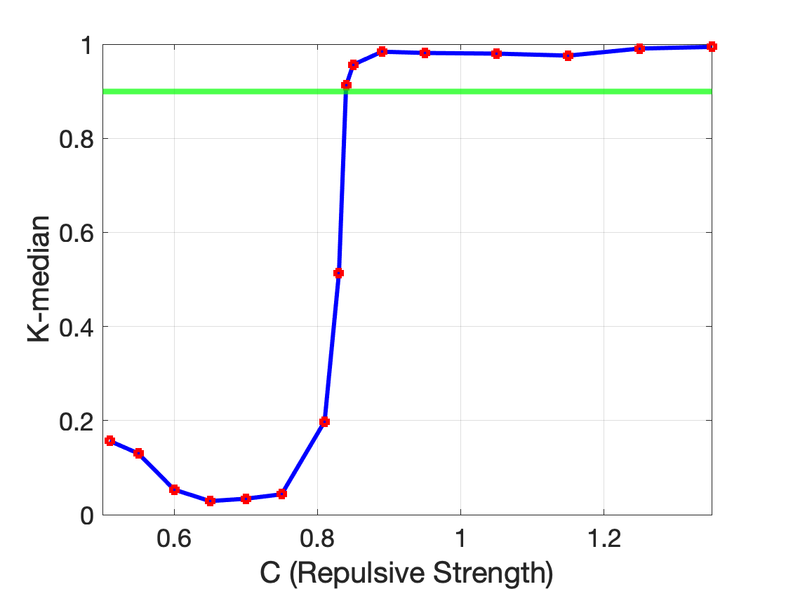
Figure 6: 0-1 test results obtained from plotting $K=$ median($K_{a})$ for different values of the coupling strength C. We interpret our result as chaotic for $K\geq 0.9$, indicated by green horizontal line.

V The level of embedding of one swarm in another: Constrained Correlation Embedding

In addition to detecting chaotic behaviors and categorizing dynamics state of milling after the collision, we are interested to see the level of complexity of interaction between the two swarmsby looking at how one swarm embeds itself in another in a similar way as shown in the appendix of previous work Schwartz, Edwards, and Hindes (2021), the idea of which originated from fractal dimension. Fractal dimension was developed as a way to quantify complexity of nature in relatively simple mathematical equations Mandelbrot, Freeman, and Company (1983). The estimation of the complexity becomes difficult in the case of the systems in which many factors of nonlinear interactions occur. We use the notion of dimension in a locally constrained manner to evaluate and quantify the level of interaction between two swarms, calling it“constrained correlation embedding.”

Without loss of generality, we count the number of agents of swarm A in a local neighborhood of an agent of swarm B. Let $N$ be a total number of agents in each Swarm. For an agent $a_{i}\in A$ and an agent $b_{j}\in B$, with the radius of a neighborhood $\epsilon$, we define

$$f(a_{i},b_{j},\epsilon)=\begin{cases}1,\;\text{ if }||a_{i}-b_{j}||<&\epsilon,\\ 0,\;\text{ if }||a_{i}-b_{j}||\geq&\epsilon.\end{cases}$$ (16)

and

$$\gamma(\epsilon)=\sum_{i\in A}^{N}\sum_{j\in B}^{N}f(a_{i},b_{j},\epsilon).$$ (17)

$\gamma(\epsilon)$ is the total count of red agents within an $\epsilon$ neighborhood of each agent of swarm B. We vary the radius of $\epsilon$ L times, and aim to see how the relative inclusion grows by plotting log of $\gamma(\epsilon)$versus log of $\epsilon$. As the value of $\epsilon$ grows, the number of agents from swarm A in the $\epsilon$ ball centered on an agent from swarm B grows as the power law $\gamma(\epsilon)\propto\epsilon^{d}$. The log-log plot behaves almost linearly until it saturates out for a large $\epsilon$. The curve saturates at large $\epsilon$ because the $\epsilon$ balls will then engulf the whole swarm thus it cannot grow any further. At extremely small values of $\epsilon$, the only inclusion in each $\epsilon$ is just the k-th agent from swarm B itself. For the range of $\epsilon$, let maximum distance and minimum distance of a given ith agent from swarm B with respect to all agents in swarm A be Max and Min, respectively. Using the power law, we divided the difference of Max and Min equally spaced logarithmically into 32Henry, Lovell, and Camacho (2000), i.e., $L=32$.

We computationally approximate $d$, the slope of the line from the region that is most linear in the log-log plot, and we defined it to be the contained correlation embedding, much like the way correlation dimension is obtainedGrassberger and Procaccia (1983) while it is done piece-wise Strogatz (2000) but locally. In order to evaluate the constrained correlation embedding, we sampled every 10th time steps, totaling 1800 points of the time - series data of interacting swarms consisting of 50 agents each.

First, our intuition tells us that a constrained correlation embedding should be between 1 and 2, since we are on the plane. Figure  7(A) is one representation of log- log plot at $C=0.81$ and the slope $d$ reflects an embedding that is fractal. The implication by CCE is that the agents of one swarm are embedded in another in a complicated way. Furthermore, we see from Fig. 7(B), that the embedding grows linearly between $C=0.65$ and 1.05, The steeper slopes indicate fast changes in the nature of the complexity. On the other hand, we see that the complexity of milling behaviors of a combined swarms saturates beyond the value $C=1.05$ while the complexities up to $C=1.05$ intensify for reach sampled value of $C$ from $C=0.81$. The same is true for the values of C below 0.65, which we interpreted as change of complexity that is more stable or minimal., consistent with our initial intuition.

We have seen from Fig. 6 that the milling state of two swarms exhibit chaotic motion as the value of $C$ grows. But the constrained correlation embedding further illustrates increasingly complicated motions within the chaotic region. From Fig. 7(B), In references to the supplementary material videos submitted, we have detected and identified the milling behaviors that are consistent with the constrained correlation embedding tendency of Fig. 7(B): For $C\in[0.81,0.95]$, we say the combined swarm forms fragmented milling where the swarm mills but it still maintains the grouping of two. Then for $C\in(0.95,1.35]$, combined swarm forms (true) milling, where the combined swarm becomes more even and unified. Notice that the milling at C = 0.95 still maintains grouping of 2 while repulsive strength C = 1.05 and C = 1.35, the milling behaviors changes only slightly, reflecting the steepness of the slope. (See supplementary material for videos of the dynamics with varying repulsion.)

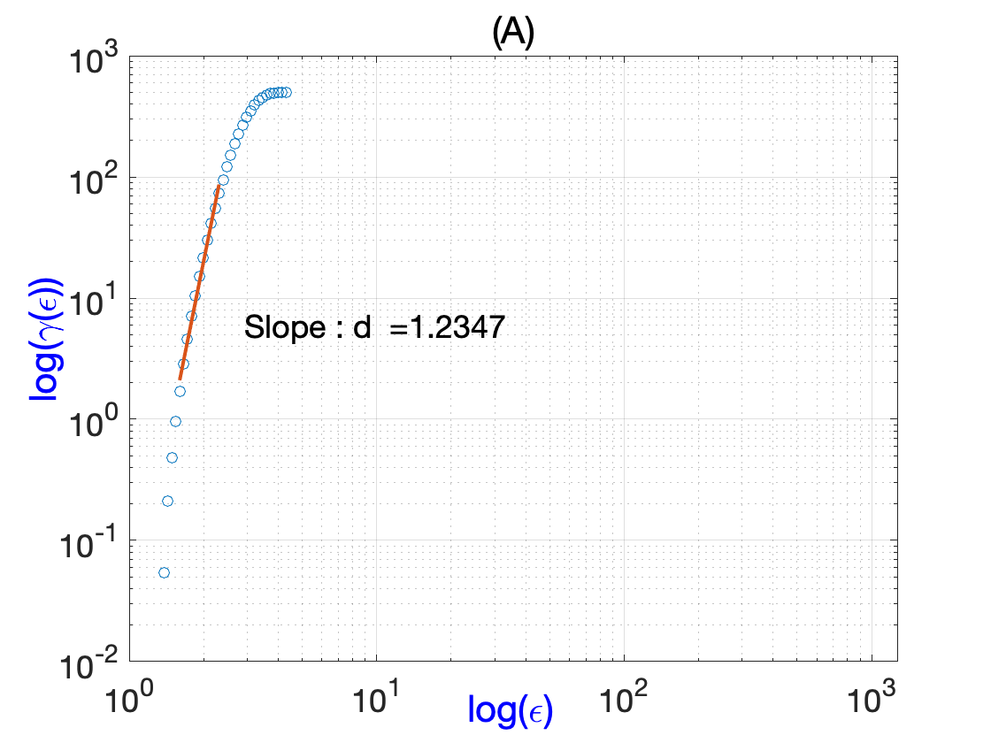
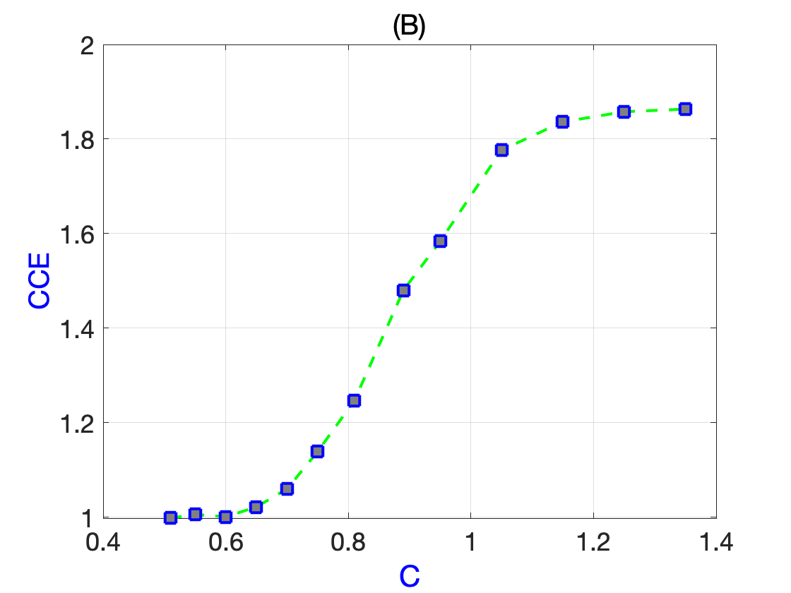
Figure 7: (A) Constrained Correlation Embedding (CCE) for Repulsive strength C = 0.81, (B) CCE as a function of repulsive strength C.

VI Conclusion, Discussion and Future Works

We have studied post collision dynamics of combined swarm milling states. We began our analysis by extracting the essential modal dynamics-information from swarm collision data through a Karhunen-Loeve decomposition, then performed the 0-1 test for detecting chaos; we further defined and used a constrained correlation method to see the level of local complexity as a result of two swarms colliding. We have observed that a motion of periodic orbits transitions to a motion on a torus before undergoing chaotic motion for a given range of repulsion strength. For a single swarm dynamics, we have not observed such transition to chaos using Eqs. 1,2. Furthermore, our constrained correlation embedding method reveals that formation of the milling itself becomes more complex as a function of repulsive strength. CCE enables us to categorize the milling as fragmented or true milling based on the range of repulsive strength; where the simple binary test of chaos does not reveal the details of the complexity of the milling within chaotic region.

One of the implications of the current result is that there is most likely a limitation to the theoretical mean-field analysis of the particular interacting swarms systems we studied. The KL mode decomposition shows that the modes needed to capture 95 percent of the data variance increases drastically as the value of $C$ increases, and reveals a sharp transition to high dimensions. It might be an indication that the bifurcation analysis at higher values of $C$ with the usual mean-field theory not be very meaningful due to spatial averaging. We likely need to come up with a way that is more accommodating to the complexity and dynamical structural analysis of interacting swarms.

Our future work includes the investigation of the sequence that leads to chaos, as we have observed and have shown a possible Ruelle-Takens-Newhouse scenario of chaos Gonzalez-Albaladejo, Carpio, and Bonilla (2023) due to torus breakup, which is accompanied by a large change in modal dimension as a function of $C$. Moreover, knowing the region of chaos in the swarm systems is a great advantage from a control theoretical point of view Rosalie et al. (2016). We may be able to stabilize unstable states of colliding swarm dynamics using various control techniques, such as those used in Triandaf and Schwartz (1997), which is based on analyzing the dynamics of the main coherent structure in the data represented by the highest energy of KL mode.

Lastly, recall that from Eq. 4, KL mode decomposition relies on space - time splitting hypothesis. The concept of space-time splitting refers to the separation of variables into spatial and temporal components. In some cases, there are dynamical systems in which the temporal behavior of the system cannot be separated from its spatial behavior. In other words, the evolution of the system over time is inherently tied to the way in which it moves through space, such as nonlinear waves Vadas and Nicolls (2012), turbulence flowManneville (1991) and chemical reactions Grasselli, Bertoni, and Goldoni (2015). Overall, many real-world dynamical systems do not exhibit the property of space-time splitting Kirby (2000). Nonetheless, in the current work, we present a case where the rapid change in KL dimension correlates with a dramatic transition in dynamical complexity. Combined with the constrained correlation embedding analysis, we have enhanced insights to the complexity analysis of chaos.

VII SUPPLEMENTARY MATERIAL

The videos show the milling state of a combined swarms consisting of N=50 agents each. The values of Repulsive strength C for five videos are: 0.51, 0.70, 0.89, 0.95, 1.05 and 1.35 respectively. Other representative parameters for generating milling states after collision are fixed, as mentioned in Sec. II.

VIII ACKNOWLEDGMENTS

SK, JH and IBS were supported by the U.S. Naval Research Laboratory funding (N0001419WX00055), the Office of Naval Research (N0001419WX01166) and (N0001419WX01322), and the Naval Innovative Science and Engineering.

References

- Li and Sayed (2012) J. Li and A. H. Sayed, “Modeling bee swarming behavior through diffusion adaptation with asymmetric information sharing,” EURASIP Journal on Advances in Signal Processing 2012, 18 (2012).
- Theraulaz et al. (2002) G. Theraulaz, E. Bonabeau, S. C. Nicolis, R. V. Solé, V. Fourcassié, S. Blanco, R. Fournier, J.-L. Joly, P. Fernández, A. Grimal, P. Dalle, and J.-L. Deneubourg, “Spatial patterns in ant colonies,” Proceedings of the National Academy of Sciences 99, 9645–9649 (2002), https://www.pnas.org/content/99/15/9645.full.pdf .
- Li et al. (2017) H. Li, C. Feng, H. Ehrhard, Y. Shen, B. Cobos, F. Zhang, K. Elamvazhuthi, S. Berman, M. Haberland, and A. L. Bertozzi, “Decentralized stochastic control of robotic swarm density: Theory, simulation, and experiment,” in 2017 IEEE/RSJ International Conference on Intelligent Robots and Systems (IROS) (2017) pp. 4341–4347.
- Ramachandran, Elamvazhuthi, and Berman (2018) R. K. Ramachandran, K. Elamvazhuthi, and S. Berman, “An optimal control approach to mapping gps-denied environments using a stochastic robotic swarm,” in Robotics Research: Volume 1, edited by A. Bicchi and W. Burgard (Springer International Publishing, Cham, 2018) pp. 477–493.
- Szwaykowska, Schwartz, and Carr (2018) K. Szwaykowska, I. B. Schwartz, and T. W. Carr, “State transitions in generic systems with asymmetric noise and communication delay,” in 2018 11th International Symposium on Mechatronics and its Applications (ISMA) (2018) pp. 1–6.
- Edwards et al. (2020) V. Edwards, P. deZonia, M. A. Hsieh, J. Hindes, I. Triandaf, and I. B. Schwartz, “Delay induced swarm pattern bifurcations in mixed reality experiments,” Chaos 30, 073126 (2020).
- Hindes et al. (2021) J. Hindes, V. Edwards, M. A. Hsieh, and I. B. Schwartz, “Critical transition for colliding swarms,” Phys. Rev. E 103, 062602 (2021).
- Levine, Rappel, and Cohen (2000) H. Levine, W. J. Rappel, and I. Cohen, Phys. Rev. E 63, 017101 (2000).
- Minguzzi (2015) E. Minguzzi, “Rayleigh’s dissipation function at work,” European Journal of Physics 36, 035014 (2015).
- D’Orsogna et al. (2006) M. R. D’Orsogna, Y. L. Chuang, A. L. Bertozzi, and L. S. Chayes, Phys. Rev. Lett. 96, 104302 (2006).
- y Teran-Romero, Forgoston, and Schwartz (2012) L. M. y Teran-Romero, E. Forgoston, and I. B. Schwartz, “Coherent pattern prediction in swarms of delay-coupled agents,” IEEE Transactions on Robotics 28, 1034–1044 (2012).
- Ling et al. (2019) H. Ling, G. E. Mclvor, K. van der Vaart, R. T. Vaughan, A. Thornton, and N. T. Ouellette, “Local interactions and their group-level consequences in flocking jackdaws,” Proceedings of the Royal Society B: Biological Sciences 286, 20190865 (2019).
- Mier-y Teran-Romero, Forgoston, and Schwartz (2011) L. Mier-y Teran-Romero, E. Forgoston, and I. B. Schwartz, “Noise, bifurcations, and modeling of interacting particle systems,” IIEEE/RSJ International Conference on Intelligent Robots and Systems , 3905–3910 (2011).
- Szwaykowska et al. (2016) K. Szwaykowska, I. B. Schwartz, L. Mier-y Teran Romero, C. R. Heckman, D. Mox, and M. A. Hsieh, “Collective motion patterns of swarms with delay coupling: Theory and experiment,” Phys. Rev. E 93, 032307 (2016).
- Schwartz et al. (2020) I. B. Schwartz, V. Edwards, S. Kamimoto, K. Kasraie, M. Ani Hsieh, I. Triandaf, and J. Hindes, “Torus bifurcations of large-scale swarms having range dependent communication delay,” Chaos: An Interdisciplinary Journal of Nonlinear Science 30, 051106 (2020).
- Armbruster, Martin, and Thatcher (2017) D. Armbruster, S. Martin, and A. Thatcher, “Elastic and inelastic collisions of swarms,” Physica D: Nonlinear Phenomena 344, 45–57 (2017).
- Kolon and Schwartz (2018) C. Kolon and I. B. Schwartz, “The dynamics of interacting swarms,” arXiv preprint arXiv:1803.08817 (2018).
- Sartoretti and Hongler (2016) G. Sartoretti and M.-O. Hongler, “Interacting brownian swarms: Some analytical results,” Entropy 18 (2016), 10.3390/e18010027.
- Chipade and Panagou (2019) V. S. Chipade and D. Panagou, “Herding an adversarial swarm in an obstacle environment,” in 2019 IEEE 58th Conference on Decision and Control (CDC) (2019) pp. 3685–3690.
- Chipade and Panagou (2020) V. S. Chipade and D. Panagou, “Multi-swarm herding: Protecting against adversarial swarms,” in 2020 59th IEEE Conference on Decision and Control (CDC) (2020) pp. 5374–5379.
- Park et al. (2018) H. Park, Q. Gong, W. Kang, C. Walton, and I. Kaminer, “Observability analysis of an adversarial swarm-a cooperation strategy,” in 2018 IEEE 14th International Conference on Control and Automation (ICCA) (2018) pp. 992–997.
- Albi et al. (2014) G. Albi, D. Balaguè, J. A. Carrillo, and J. von Brecht, “Stability analysis of flock and mill rings for 2nd order models in swarming,” SIAM J. Appl. Math. 74, 794 (2014).
- Bernoff and Topaz (2011) A. Bernoff and C. Topaz, SIAM Journal of Applied Dynamical Systems 10, 212 (2011).
- Hindes et al. (2020) J. Hindes, V. Edwards, S. Kamimoto, I. Triandaf, and I. B. Schwartz, “Unstable modes and bistability in delay-coupled swarms,” Physical Review E 101, 042202 (2020).
- Chuang et al. (2007) Y.-L. Chuang, Y. R. Huang, M. R. D’Orsogna, and A. L. Bertozzi, “Multi-vehicle flocking: Scalability of cooperative control algorithms using pairwise potentials,” in Proceedings 2007 IEEE International Conference on Robotics and Automation (2007) pp. 2292–2299.
- Landau and Lifshitz (1976) L. D. Landau and E. M. Lifshitz, Mechanics, Third Edition: Volume 1 (Course of Theoretical Physics), 3rd ed. (Butterworth-Heinemann, 1976).
- Sirovich (1987) L. Sirovich, “Turbulence and the dynamics of coherent structures. i. coherent structures,” Quarterly of Applied Mathematics 45, 561–571 (1987).
- Jolliffe and Cadima (2016) I. T. Jolliffe and J. Cadima, “Principal component analysis: a review and recent developments,” Philosophical Transactions of the Royal Society A: Mathematical, Physical and Engineering Sciences 374, 20150202 (2016).
- Rao and Ahmed (1976) K. Rao and N. Ahmed, “Orthogonal transforms for digital signal processing,” in ICASSP ’76. IEEE International Conference on Acoustics, Speech, and Signal Processing, Vol. 1 (1976) pp. 136–140.
- Gottwald and Melbourne (2004) A. Gottwald and I. Melbourne, “A new test for chaos in deterministic systems,” Proc. R. Soc. London A , 603–611 (2004).
- Gottwald and Melbourne (2009a) G. A. Gottwald and I. Melbourne, “On the implementation of the 0-1 test for chaos,” SIAM Journal on Applied Dynamical Systems 8, 129–145 (2009a), https://doi.org/10.1137/080718851 .
- Gottwald and Melbourne (2009b) G. A. Gottwald and I. Melbourne, “On the validity of the 0?1 test for chaos,” Nonlinearity 22, 1367 (2009b).
- Melbourne and Gottwald (2007) I. Melbourne and G. A. Gottwald, “Power spectra for deterministic chaotic dynamical systems,” Nonlinearity 21, 179 (2007).
- (34) P. Matthews, “0 - 1 test for chaos,” MathWorks .
- Gottwald and Melbourne (2008) G. A. Gottwald and I. Melbourne, “Comment on “reliability of the 0-1 test for chaos”,” Phys. Rev. E 77, 028201 (2008).
- Schwartz, Edwards, and Hindes (2021) I. B. Schwartz, V. Edwards, and J. Hindes, “Interacting Swarm Sensing and Stabilization,” arXiv e-prints , arXiv:2106.01824 (2021), arXiv:2106.01824 [nlin.AO] .
- Mandelbrot, Freeman, and Company (1983) B. Mandelbrot, W. H. Freeman, and Company, The Fractal Geometry of Nature, Einaudi paperbacks (Henry Holt and Company, 1983).
- Henry, Lovell, and Camacho (2000) B. Henry, N. Lovell, and F. Camacho, “Nonlinear dynamics time series analysis,” in Nonlinear Biomedical Signal Processing (John Wiley and Sons, Ltd, 2000) Chap. 1, pp. 1–39, https://onlinelibrary.wiley.com/doi/pdf/10.1109/9780470545379.ch1 .
- Grassberger and Procaccia (1983) P. Grassberger and I. Procaccia, “Measuring the strangeness of strange attractors,” Physica D: Nonlinear Phenomena 9, 189–208 (1983).
- Strogatz (2000) S. H. Strogatz, Nonlinear Dynamics and Chaos: With Applications to Physics, Biology, Chemistry and Engineering (Westview Press, 2000).
- Gonzalez-Albaladejo, Carpio, and Bonilla (2023) R. Gonzalez-Albaladejo, A. Carpio, and L. L. Bonilla, “Scale-free chaos in the confined vicsek flocking model,” Phys. Rev. E 107, 014209 (2023).
- Rosalie et al. (2016) M. Rosalie, G. Danoy, S. Chaumette, and P. Bouvry, “From random process to chaotic behavior in swarms of uavs,” Proceedings of the 6th ACM Symposium on Development and Analysis of Intelligent Vehicular Networks and Applications (2016).
- Triandaf and Schwartz (1997) I. Triandaf and I. B. Schwartz, “Karhunen-loeve mode control of chaos in a reaction-diffusion process,” Phys. Rev. E 56, 204–212 (1997).
- Vadas and Nicolls (2012) S. L. Vadas and M. J. Nicolls, “The phases and amplitudes of gravity waves propagating and dissipating in the thermosphere: Theory,” Journal of Geophysical Research: Space Physics 117 (2012), https://doi.org/10.1029/2011JA017426, https://agupubs.onlinelibrary.wiley.com/doi/pdf/10.1029/2011JA017426 .
- Manneville (1991) P. Manneville, “From chaos to turbulence in fluid dynamics,” in Engineering Applications of Dynamics of Chaos, edited by W. Szemplinska-Stupnicka and H. Troger (Springer Vienna, Vienna, 1991) pp. 67–137.
- Grasselli, Bertoni, and Goldoni (2015) F. Grasselli, A. Bertoni, and G. Goldoni, “Space- and time-dependent quantum dynamics of spatially indirect excitons in semiconductor heterostructures.” The Journal of chemical physics 142 3, 034701 (2015).
- Kirby (2000) M. Kirby, “Geometric data analysis: An empirical approach to dimensionality reduction and the study of patterns,” (2000).