Better Private Linear Regression Through
Better Private Feature Selection

Abstract

Existing work on differentially private linear regression typically assumes that end users can precisely set data bounds or algorithmic hyperparameters. End users often struggle to meet these requirements without directly examining the data (and violating privacy). Recent work has attempted to develop solutions that shift these burdens from users to algorithms, but they struggle to provide utility as the feature dimension grows. This work extends these algorithms to higher-dimensional problems by introducing a differentially private feature selection method based on Kendall rank correlation. We prove a utility guarantee for the setting where features are normally distributed and conduct experiments across 25 datasets. We find that adding this private feature selection step before regression significantly broadens the applicability of “plug-and-play” private linear regression algorithms at little additional cost to privacy, computation, or decision-making by the end user.

1 Introduction

Differentially private [10] algorithms employ carefully calibrated randomness to obscure the effect of any single data point. Doing so typically requires an end user to provide bounds on input data to ensure the correct scale of noise. However, end users often struggle to provide such bounds without looking at the data itself [27], thus nullifying the intended privacy guarantee. This has motivated the development of differentially private algorithms that do not require these choices from users.

To the best of our knowledge, two existing differentially private linear regression algorithms satisfy this “plug-and-play” requirement: 1) the Tukey mechanism [2], which combines propose-test-release with an exponential mechanism based on Tukey depth, and 2) Boosted AdaSSP [30], which applies gradient boosting to the AdaSSP algorithm introduced by Wang [34]. We refer to these methods as, respectively, $\mathsf{Tukey}$ and $\mathsf{BAS}$. Neither algorithm requires data bounds, and both feature essentially one chosen parameter (the number of models $m$ for $\mathsf{Tukey}$, and the number of boosting rounds $T$ for $\mathsf{BAS}$) which admits simple heuristics without tuning. $\mathsf{Tukey}$ obtains strong empirical results when the number of data points $n$ greatly exceeds the feature dimension $d$ [2], while $\mathsf{BAS}$ obtains somewhat weaker performance on a larger class of datasets [30].

Nonetheless, neither algorithm provides generally strong utility on its own. Evaluated over a collection of 25 linear regression datasets taken from Tang et al. [30], $\mathsf{Tukey}$ and $\mathsf{BAS}$ obtain coefficient of determination $R^{2}>0$ on only four (see Section 4); for context, a baseline of $R^{2}=0$ is achieved by the trivial constant predictor, which simply outputs the mean label. These results suggest room for improvement for practical private linear regression.

1.1 Our Contributions

We extend existing work on private linear regression by adding a preprocessing step that applies private feature selection. At a high level, this strategy circumvents the challenges of large feature dimension $d$ by restricting attention to $k\ll d$ carefully selected features. We initiate the study of private feature selection in the context of “plug-and-play” private linear regression and make two concrete contributions:

1. We introduce a practical algorithm, $\mathsf{DPKendall}$, for differentially private feature selection (Section 3). $\mathsf{DPKendall}$ uses Kendall rank correlation [20] and only requires the user to choose the number $k$ of features to select. It satisfies $\varepsilon$-DP and, given $n$ samples with $d$-dimensional features, runs in time $O(dkn\log(n))$ (Theorem 3.4). We also provide a utility guarantee when the features are normally distributed (Theorem 3.8).

2. We conduct experiments across 25 datasets (Section 4), with $k$ fixed at $5$ and $10$. These compare $\mathsf{Tukey}$ and $\mathsf{BAS}$ without feature selection, with $\mathsf{SubLasso}$ feature selection [21], and with $\mathsf{DPKendall}$ feature selection. Using $(\ln(3),10^{-5})$-DP to cover both private feature selection and private regression, we find at $k=5$ that adding $\mathsf{DPKendall}$ yields $R^{2}>0$ on 56% of the datasets. Replacing $\mathsf{DPKendall}$ with $\mathsf{SubLasso}$ drops the rate to 40% of datasets, and omitting feature selection entirely drops it further to 16%.

In summary, we suggest that $\mathsf{DPKendall}$ significantly expands the applicability and utility of practical private linear regression.

1.2 Related Work

The focus of this work is practical private feature selection applied to private linear regression. We therefore refer readers interested in a more general overview of the private linear regression literature to the discussions of Amin et al. [2] and Tang et al. [30].

Several works have studied private sparse linear regression [21, 31, 17, 29]. However, Jain and Thakurta [17] and Talwar et al. [29] require an $\ell_{\infty}$ bound on the input data, and the stability test that powers the feature selection algorithm of Thakurta and Smith [31] requires the end user to provide granular details about the optimal Lasso model. These requirements are significant practical obstacles. An exception is the work of Kifer et al. [21]. Their algorithm first performs feature selection using subsampling and aggregation of non-private Lasso models. This feature selection method, which we call $\mathsf{SubLasso}$, only requires the end user to select the number of features $k$. To the selected features, Kifer et al. [21] then apply objective perturbation to privately optimize the Lasso objective. As objective perturbation requires the end user to choose parameter ranges and provides a somewhat brittle privacy guarantee contingent on the convergence of the optimization, we do not consider it here. Instead, our experiments combine $\mathsf{SubLasso}$ feature selection with the $\mathsf{Tukey}$ and $\mathsf{BAS}$ private regression algorithms. An expanded description of $\mathsf{SubLasso}$ appears in Section 4.2.

We now turn to the general problem of private feature selection. There is a significant literature studying private analogues of the general technique of principal component analysis (PCA) [25, 15, 8, 19, 11, 1]. Unfortunately, all of these algorithms assume some variant of a bound on the row norm of the input data. Stoddard et al. [28] studied private feature selection in the setting where features and labels are binary, but it is not clear how to extend their methods to the non-binary setting that we consider in this work. $\mathsf{SubLasso}$ is therefore the primary comparison private feature selection method in this paper. We are not aware of existing work that studies private feature selection in the specific context of “plug-and-play” private linear regression.

Finally, private rank correlation has previously been studied by Kusner et al. [23]. They derived a different, normalized sensitivity bound appropriate for their “swap” privacy setting and applied it to privately determine the causal relationship between two random variables.

2 Preliminaries

Throughout this paper, a database $D$ is a collection of labelled points $(x,y)$ where $x\in\mathbb{R}^{d}$, $y\in\mathbb{R}$, and each user contributes a single point. We use the “add-remove” form of differential privacy.

Definition 2.1 ([10]).

Databases $D,D^{\prime}$ from data domain $\mathcal{D}$ are neighbors $D\sim D^{\prime}$ if they differ in the presence or absence of a single record. A randomized mechanism $\mathcal{M}:\mathcal{D}\to\mathcal{O}$ is $(\varepsilon,\delta)$-differentially private (DP) if for all $D\sim D^{\prime}\in\mathcal{D}$ and any $S\subseteq\mathcal{O}$

$$\mathbb{P}_{\mathcal{M}}\left[\mathcal{M}(D)\in S\right]\leq e^{\varepsilon}\mathbb{P}_{\mathcal{M}}\left[\mathcal{M}(D^{\prime})\in S\right]+\delta.$$

When $\delta=0$, we say $\mathcal{M}$ is $\varepsilon$-DP.

We use basic composition to reason about the privacy guarantee obtained from repeated application of a private algorithm. More sophisticated notions of composition exist, but for our setting of relatively few compositions, basic composition is simpler and suffers negligible utility loss.

Lemma 2.2 ([10]).

Suppose that for $j\in[k]$, algorithm $\mathcal{A}_{j}$ is $(\varepsilon_{j},\delta_{j}$)-DP. Then running all $k$ algorithms is $(\sum_{j=1}^{k}\varepsilon_{j},\sum_{j=1}^{k}\delta_{j})$-DP.

Both $\mathsf{SubLasso}$ and $\mathsf{DPKendall}$ use a private subroutine for identifying the highest count item(s) from a collection, known as private top-$k$. Several algorithms for this problem exist [4, 9, 13]. We use the pure DP “peeling mechanism” based on Gumbel noise [9], as its analysis is relatively simple, and its performance is essentially identical to other variants for the relatively small $k$ used in this paper.

Definition 2.3 ([9]).

A Gumbel distribution with parameter $b$ is defined over $x\in\mathbb{R}$ by $\mathbb{P}\left[x;b\right]=\frac{1}{b}\cdot\exp\left(-\frac{x}{b}-e^{-x/b}\right)$. Given $c=(c_{1},\ldots,c_{d})\in\mathbb{R}^{d}$, $k\in\mathbb{N}$, and privacy parameter $\varepsilon$, $\mathsf{Peel}(c,k,\Delta_{\infty},\varepsilon)$ adds independent $\mathsf{Gumbel}\left(\tfrac{2k\Delta_{\infty}}{\varepsilon}\right)$ noise to each count $c_{j}$ and outputs the ordered sequence of indices with the largest noisy counts.

Lemma 2.4 ([9]).

Given $c=(c_{1},\ldots,c_{d})\in\mathbb{R}^{d}$ with $\ell_{\infty}$ sensitivity $\Delta_{\infty}$, $\mathsf{Peel}(c,k,\Delta_{\infty},\varepsilon)$ is $\varepsilon$-DP.

The primary advantage of $\mathsf{Peel}$ over generic noise addition is that, although users may contribute to $d$ counts, the added noise only scales with $k$. We note that while $\mathsf{Peel}$ requires an $\ell_{\infty}$ bound, neither $\mathsf{DPKendall}$ nor $\mathsf{SubLasso}$ needs user input to set it: regardless of the dataset, $\mathsf{DPKendall}$’s use of $\mathsf{Peel}$ has $\ell_{\infty}=3$ and $\mathsf{SubLasso}$’s use has $\ell_{\infty}=1$ (see Algorithms 1 and 2).

3 Feature Selection Algorithm

This section describes our feature selection algorithm, $\mathsf{DPKendall}$, and formally analyzes its utility. Section 3.1 introduces and discusses Kendall rank correlation, Section 3.2 describes the full algorithm, and the utility result appears in Section 3.3.

3.1 Kendall Rank Correlation

The core statistic behind our algorithm is Kendall rank correlation. Informally, Kendall rank correlation measures the strength of a monotonic relationship between two variables.

Definition 3.1 ([20]).

Given a collection of data points $(X,Y)=\{(X_{1},Y_{1}),\ldots,(X_{n},Y_{n})\}$ and $i<i^{\prime}$, a pair of observations $(X_{i},Y_{i}),(X_{i^{\prime}},Y_{i^{\prime}})$ is discordant if $(X_{i}-X_{i^{\prime}})(Y_{i}-Y_{i^{\prime}})<0$. Given data $(X,Y)$, let $d_{X,Y}$ denote the number of discordant pairs. Then the empirical Kendall rank correlation is

$$\hat{\tau}(X,Y)\coloneqq\frac{n}{2}-\frac{2d_{X,Y}}{n-1}.$$

For real random variables $X$ and $Y$, we can also define the population Kendall rank correlation by

$$\tau(X,Y)=\mathbb{P}\left[(X-X^{\prime})(Y-Y^{\prime})>0\right]-\mathbb{P}\left[(X-X^{\prime})(Y-Y^{\prime})<0\right].$$

Kendall rank correlation is therefore high when an increase in $X$ or $Y$ typically accompanies an increase in the other, low when an increase in one typically accompanies a decrease in the other, and close to 0 when a change in one implies little about the other. We typically focus on empirical Kendall rank correlation, but the population definition will be useful in the proof of our utility result.

Before discussing Kendall rank correlation in the context of privacy, we note two straightforward properties. First, for simplicity, we use a version of Kendall rank correlation that does not account for ties. We ensure this in practice by perturbing data by a small amount of continuous random noise. Second, $\tau$ has range $[-1,1]$, but (this paper’s version of) $\hat{\tau}$ has range $[-n/2,n/2]$. This scaling does not affect the qualitative interpretation and ensures that $\hat{\tau}$ has low sensitivity.

Lemma 3.2.

$\Delta(\hat{\tau})=3/2$.

Proof.

At a high level, the proof verifies that the addition or removal of a user changes the first term of $\hat{\tau}$ by at most 1/2, and the second term by at most 1.

In more detail, consider two neighboring databases $(X,Y)$ and $(X^{\prime},Y^{\prime})$. Without loss of generality, we may assume that $(X,Y)=\{(X_{1},Y_{1}),\ldots,(X_{n},Y_{n})\}$ and $(X^{\prime},Y^{\prime})=\{(X^{\prime}_{1},Y^{\prime}_{1}),\ldots,(X^{\prime}_{n+1},Y^{\prime}_{n+1})\}$ where for all $i\in[n]$ we have that $X^{\prime}_{i}=X_{i}$ and $Y^{\prime}_{i}=Y_{i}$. First, we argue that the number of discordant pairs in $(X^{\prime},Y^{\prime})$ cannot be much larger than in $(X,Y)$. By definition, we have that $d_{X^{\prime},Y^{\prime}}-d_{X,Y}=\sum_{j=1}^{n}\mathbbm{1}_{(X_{j}-X^{\prime}_{n+1})(Y_{j}-Y^{\prime}_{n+1})<0}$. In particular, this implies that $d_{X^{\prime},Y^{\prime}}-d_{X,Y}\in[0,n]$.

We can rewrite the difference in Kendall correlation between $(X,Y)$ and $(X^{\prime},Y^{\prime})$ as follows:

$$\hat{\tau}(X,Y)-\hat{\tau}(X^{\prime},Y^{\prime}) =\frac{n}{2}-\frac{2d_{X,Y}}{n-1}-\frac{n+1}{2}+\frac{2d_{X^{\prime},Y^{\prime}}}{n}$$

$$=2\left(\frac{d_{X^{\prime},Y^{\prime}}}{n}-\frac{d_{X,Y}}{n-1}\right)-\frac{1}{2}$$

$$=2\left(\frac{d_{X^{\prime},Y^{\prime}}-d_{X,Y}}{n}+\frac{d_{X,Y}}{n}-\frac{d_{X,Y}}{n-1}\right)-\frac{1}{2}$$

$$=2\frac{d_{X^{\prime},Y^{\prime}}-d_{X,Y}}{n}+2d_{X,Y}\left(\frac{1}{n}-\frac{1}{n-1}\right)-\frac{1}{2}$$

$$=2\frac{d_{X^{\prime},Y^{\prime}}-d_{X,Y}}{n}-\frac{d_{X,Y}}{{n\choose 2}}-\frac{1}{2},$$

where the final equality follows from the fact that $2(\frac{1}{n}-\frac{1}{n-1})=-1/{n\choose 2}$. Using our previous calculation, the first term is in the range $[0,2]$ and, since $d_{X,Y}\in[0,{n\choose 2}]$, the second term is in the range $[-1,0]$. It follows that

$$-\frac{3}{2}=0-1-\frac{1}{2}\leq\hat{\tau}(X,Y)-\hat{\tau}(X^{\prime},Y^{\prime})\leq 2-0-\frac{1}{2}=\frac{3}{2},$$

and therefore $|\hat{\tau}(X,Y)-\hat{\tau}(X^{\prime},Y^{\prime})|\leq 3/2$.

To show that the sensitivity is not smaller than $3/2$, consider neighboring databases $(X,Y)$ and $(X^{\prime},Y^{\prime})$ such that $d_{X,Y}=0$ and $(X^{\prime},Y^{\prime})$ contains a new point that is discordant with all points in $(X,Y)$. Then $d_{X^{\prime},Y^{\prime}}=n$ while $d_{X,Y}=0$. Then $\hat{\tau}(X,Y)-\hat{\tau}(X^{\prime},Y^{\prime})=2-0-1/2=3/2$. ∎

Turning to privacy, Kendall rank correlation has two notable strengths. First, because it is computed entirely from information about the relative ordering of data, it does not require an end user to provide data bounds. This makes it a natural complement to private regression methods that also operate without user-provided data bounds. Second, Kendall rank correlation’s sensitivity is constant, but its range scales linearly with $n$. This makes it easy to compute privately. A contrasting example is Pearson correlation, which requires data bounds to compute covariances and has sensitivity identical to its range. An extended discussion of alternative notions of correlation appears in Section 6.

Finally, Kendall rank correlation can be computed relatively quickly using a variant of merge sort.

Lemma 3.3 ([22]).

Given collection of data points $(X,Y)=\{(X_{1},Y_{1}),\ldots,(X_{n},Y_{n})\}$, $\hat{\tau}(X,Y)$ can be computed in time $O(n\log(n))$.

3.2 $\mathsf{DPKendall}$

Having defined Kendall rank correlation, we now describe our private feature selection algorithm, $\mathsf{DPKendall}$. Informally, $\mathsf{DPKendall}$ balances two desiderata: 1) selecting features that correlate with the label, and 2) selecting features that do not correlate with previously selected features. Prioritizing only the former selects for redundant copies of a single informative feature, while prioritizing only the latter selects for features that are pure noise.

In more detail, $\mathsf{DPKendall}$ consists of $k$ applications of $\mathsf{Peel}$ to select a feature that is correlated with the label and relatively uncorrelated with the features already chosen. Thus, letting $S_{t}$ denote the set of $t-1$ features already chosen in round $t$, each round attempts to compute

$$\max_{j\not\in S_{t}}\left(|\hat{\tau}(X_{j},Y)|-\frac{1}{t-1}\sum_{j^{\prime}\in S_{t}}|\hat{\tau}(X_{j},X_{j^{\prime}})|\right).$$ (1)

The $\tfrac{1}{t-1}$ scaling ensures that the sensitivity of the overall quantity remains fixed at $\tfrac{3}{2}$ in the first round and 3 in the remaining rounds. Note that in the first round we take second term to be 0, and only label correlation is considered.

1:  Input: Examples $D=\{(X_{i},Y_{i})\}_{i=1}^{n}$, number of selected features $k$, privacy parameter $\varepsilon$

2:  for $j=1,\ldots,d$ do

3:     Compute $\hat{\tau}_{j}^{Y}=|\hat{\tau}(X_{j},Y)|$

4:  Initialize $S=\emptyset$

5:  Initialize $\hat{\tau}=\hat{\tau}^{Y}\in\mathbb{R}^{d}$

6:  Initialize $\hat{\tau}^{X}=0\in\mathbb{R}^{d}$

7:  for $t=1,\ldots,k$ do

8:     Set $\Delta_{\infty}=\tfrac{3}{2}+\tfrac{3}{2}\cdot\mathbbm{1}_{t>1}$

9:     Set $s_{t}=\mathsf{Peel}\left(\hat{\tau}^{Y}-\tfrac{\hat{\tau}^{X}}{t-1},1,\Delta_{\infty},\tfrac{\varepsilon}{k}\right)$

10:     Expand $S=S\cup s_{t}$

11:     Update $\hat{\tau}_{s_{t}}^{Y}=-\infty$

12:     for $j\not\in S$ do

13:        Update $\hat{\tau}_{j}^{X}=\hat{\tau}_{j}^{X}-|\hat{\tau}(X_{j},X_{s_{t}})|$

14:  Return $S$

Algorithm 1 $\mathsf{DPKendall}(D,k,\varepsilon)$

Pseudocode for $\mathsf{DPKendall}$ appears in Algorithm 1. Its runtime and privacy are easy to verify.

Theorem 3.4.

$\mathsf{DPKendall}$ runs in time $O(dkn\log(n))$ and satisfies $\varepsilon$-DP.

Proof.

By Lemma 3.3, each computation of Kendall rank correlation takes time $O(n\log(n))$, so Line 2’s loop takes time $O(dn\log(n))$, as does each execution of Line 12’s loop. Each call to $\mathsf{Peel}$ requires $O(d)$ samples of Gumbel noise and thus contributes $O(dk)$ time overall. The loop in Line 7 therefore takes time $O(dkn\log(n))$. The privacy guarantee follows from Lemmas 2.4 and 3.2. ∎

For comparison, standard OLS on $n$ samples of data with $d$ features requires time $O(d^{2}n)$; $\mathsf{DPKendall}$ is asymptotically no slower as long as $n\leq O(2^{d/k})$. Since we typically take $k\ll d$, $\mathsf{DPKendall}$ is computationally “free” in many realistic data settings.

3.3 Utility Guarantee

The proof of $\mathsf{DPKendall}$’s utility guarantee combines results about population Kendall rank correlation (Lemma 3.5), empirical Kendall rank correlation concentration (Lemma 3.6), and the accuracy of $\mathsf{Peel}$ (Lemma 3.7). The final guarantee (Theorem 3.8) demonstrates that $\mathsf{DPKendall}$ selects useful features even in the presence of redundant features.

We start with the population Kendall rank correlation guarantee.

Lemma 3.5.

Suppose that $X_{1},\ldots,X_{k}$ are independent random variables where $X_{j}\sim N(\mu_{j},\sigma_{j}^{2})$. Let $\xi\sim N(0,\sigma_{e}^{2})$ be independent noise. Then if the label is generated by $Y=\sum_{j=1}^{k}\beta_{j}X_{j}+\xi$, for any $j^{*}\in[k]$,

$$\tau(X_{j^{*}},Y)=\frac{2}{\pi}\cdot\arctan{\frac{\beta_{j^{*}}\sigma_{j^{*}}}{\sqrt{\sum_{j\neq j^{*}}\beta_{j}^{2}\sigma_{j}^{2}+\sigma_{e}^{2}}}}.$$

Proof.

Recall from Definition 3.1 the population formulation of $\tau$,

$$\tau(X,Y)=\mathbb{P}\left[(X-X^{\prime})(Y-Y^{\prime})>0\right]-\mathbb{P}\left[(X-X^{\prime})(Y-Y^{\prime})<0\right]$$ (2)

where $X$ and $X^{\prime}$ are i.i.d., as are $Y$ and $Y^{\prime}$. In our case, we can define $Z=\sum_{j\neq j^{*}}\beta_{j}X_{j}+\xi$ and rewrite the first term of Equation 2 for our setting as

$$\int_{0}^{\infty}f_{X_{j^{*}}-X_{j^{*}}^{\prime}}(t)\cdot[1-F_{Z-Z^{\prime}}(-\beta_{j^{*}}t)]dt+\int_{-\infty}^{0}f_{X_{j^{*}}-X_{j^{*}}^{\prime}}(t)\cdot F_{Z-Z^{\prime}}(-\beta_{j^{*}}t)dt.$$ (3)

where $f_{A}$ and $F_{A}$ denote densities and cumulative distribution functions of random variable $A$, respectively. Since the relevant distributions are all Gaussian, $X_{j^{*}}-X_{j^{*}}^{\prime}\sim N(0,2\sigma_{j^{*}}^{2})$ and $Z-Z^{\prime}\sim N(0,2[\sum_{j\neq j^{*}}\beta_{j}^{2}\sigma_{j}^{2}+\sigma_{e}^{2}])$. For neatness, shorthand $\sigma^{2}=2\sigma_{j^{*}}^{2}$ and $\sigma_{-1}^{2}=2[\sum_{j\neq j^{*}}\beta_{j}^{2}\sigma_{j}^{2}+\sigma_{e}^{2}]$. Then if we let $\phi$ denote the PDF of a standard Gaussian and $\Phi$ the CDF of a standard Gaussian, Equation 3 becomes

$$\ \int_{0}^{\infty}\frac{1}{\sigma}\phi(t/\sigma)\cdot[1-\Phi(-\beta_{j^{*}}t/\sigma_{-1})]dt+\int_{-\infty}^{0}\frac{1}{\sigma}\phi(t/\sigma)\Phi(-\beta_{j^{*}}t/\sigma_{-1})dt$$

$$= \ \frac{1}{\sigma}\left[\int_{0}^{\infty}\phi(t/\sigma)\Phi(\beta_{j^{*}}t/\sigma_{-1})dt+\int_{-\infty}^{0}\phi(-t/\sigma)\Phi(-\beta_{j^{*}}t/\sigma_{-1})dt\right]$$

$$= \ \frac{2}{\sigma}\int_{0}^{\infty}\phi(t/\sigma)\Phi(\beta_{j^{*}}t/\sigma_{-1})dt.$$

We can similarly analyze the second term of Equation 2 to get

$$\ \int_{0}^{\infty}f_{X_{j^{*}}-X_{j^{*}}^{\prime}}(t)\cdot F_{Z-Z^{\prime}}(-\beta_{j^{*}}t)dt+\int_{-\infty}^{0}f_{X_{j^{*}}-X_{j^{*}}^{\prime}}(t)\cdot[1-F_{Z-Z^{\prime}}(-\beta_{j^{*}}t)]dt$$

$$= \ \int_{0}^{\infty}\frac{1}{\sigma}\phi(t/\sigma)\Phi(-\beta_{j^{*}}t/\sigma_{-1})dt+\int_{-\infty}^{0}\frac{1}{\sigma}\phi(t/\sigma)\Phi(\beta_{j^{*}}t/\sigma_{-1})dt$$

$$= \ \frac{2}{\sigma}\int_{-\infty}^{0}\phi(t/\sigma)\Phi(\beta_{j^{*}}t/\sigma_{-1})dt.$$

Using both results, we get

$$\tau(X_{1},Y)= \ \frac{2}{\sigma}\left[\int_{0}^{\infty}\phi(t/\sigma)\Phi(\beta_{j^{*}}t/\sigma_{-1})dt-\int_{-\infty}^{0}\phi(t/\sigma)\Phi(\beta_{j^{*}}t/\sigma_{-1})dt\right]$$

$$= \ \frac{2}{\sigma}\left[\int_{0}^{\infty}\phi(t/\sigma)\Phi(\beta_{j^{*}}t/\sigma_{-1})dt-\int_{0}^{\infty}\phi(t/\sigma)[1-\Phi(\beta_{j^{*}}t/\sigma_{-1})]dt\right]$$

$$= \ \frac{4}{\sigma}\int_{0}^{\infty}\phi(t/\sigma)\Phi(\beta_{j^{*}}t/\sigma_{-1})dt-1$$

$$= \ \frac{4}{\sigma}\cdot\frac{\sigma}{2\pi}\left(\frac{\pi}{2}+\arctan{\frac{\beta_{j^{*}}\sigma}{\sigma_{-1}}}\right)-1$$

$$= \ \frac{2}{\pi}\cdot\arctan{\frac{\beta_{j^{*}}\sigma}{\sigma_{-1}}}.$$

where the third equality uses $\int_{0}^{\infty}\phi(t/\sigma)dt=\frac{\sigma}{2}$ and the fourth equality comes from Equation 1,010.4 of Owen [26]. Substituting in the values of $\sigma$ and $\sigma_{-1}$ yields the claim. ∎

To interpret this result, recall that $\tau\in[-1,1]$ and $\arctan$ has domain $\mathbb{R}$, is odd, and has $\lim_{x\to\infty}\arctan{x}=\pi/2$. Lemma 3.5 thus says that if we fix the other $\sigma_{j}$ and $\sigma_{e}$ and take $\sigma_{j^{*}}\to\infty$, $\tau(X_{j^{*}},Y)\to\mathsf{sign}\left(\beta_{j^{*}}\right)$ as expected. The next step is to verify that $\hat{\tau}$ concentrates around $\tau$.

Lemma 3.6 (Lemma 1 [3]).

Given $n$ observations each of random variables $X$ and $Y$, with probability $1-\eta$,

$$|\hat{\tau}(X,Y)-\frac{n}{2}\cdot\tau(X,Y)|\leq\sqrt{8n\ln(2/\eta)}.$$

Finally, we state a basic accuracy result for the Gumbel noise employed by $\mathsf{Peel}$.

Lemma 3.7.

Given i.i.d. random variables $X_{1},\ldots,X_{d}\sim\mathsf{Gumbel}\left(b\right)$, with probability $1-\eta$,

$$\max_{j\in[d]}|X_{j}|\leq b\ln\left(\frac{2d}{\eta}\right).$$

Proof.

Recall from Definition 2.3 that $\mathsf{Gumbel}\left(b\right)$ has density $f(x)=\frac{1}{b}\cdot\exp\left(-\frac{x}{b}-e^{-x/b}\right)$. Then $\frac{f(x)}{f(-x)}=\exp\left(-\frac{x}{b}-e^{-x/b}-\frac{x}{b}+e^{x/b}\right)$. For $z\geq 0$, by $e^{z}=\sum_{n=0}^{\infty}\frac{z^{n}}{n!}$,

$$2z+e^{-z}\leq 2z+1-z+\frac{z^{2}}{2}=1+z+\frac{z^{2}}{2}\leq e^{z}$$

so since $b\geq 0$, $f(x)\geq f(-x)$ for $x\geq 0$. Letting $F(z)=\exp(-\exp(-z/b))$ denote the CDF for $\mathsf{Gumbel}\left(b\right)$, it follows that for $z\geq 0$, $1-F(z)\geq F(-z)$. Thus the probability that $\max_{j\in[d]}|X_{j}|$ exceeds $t$ is upper bounded by $2d(1-F(t))$. The claim then follows from rearranging the inequality

$$2d(1-F(t))\leq \ \eta$$

$$1-\frac{\eta}{2d}\leq \ F(t)$$

$$1-\frac{\eta}{2d}\leq \ \exp(-\exp(-t/b))$$

$$\ln\left(1-\frac{\eta}{2d}\right)\leq \ -\exp(-t/b)$$

$$-b\ln\left(-\ln\left(1-\frac{\eta}{2d}\right)\right)\leq \ t$$

$$b\ln\left(\frac{1}{-\ln(1-\eta/[2d])}\right)\leq \ t$$

and using $-\ln(1-x)=\sum_{i=1}^{\infty}x^{i}/i\geq x$. ∎

We now have the tools necessary for the final result.

Theorem 3.8.

Suppose that $X_{1},\ldots,X_{k}$ are independent random variables where each $X_{j}\sim N(\mu_{j},\sigma_{j}^{2})$. Suppose additionally that of the remaining $d-k$ random variables, for each $j\in[k]$, $n_{j}$ are copies of $X_{j}$, where $\sum_{j=1}^{k}n_{j}\leq d-k$. For each $j\in[k]$, let $S_{j}$ denote the set of indices consisting of $j$ and the indices of its copies. Then if the label is generated by $Y=\sum_{j=1}^{k}\beta_{j}X_{j}+\xi$ where $\xi\sim N(0,\sigma_{e}^{2})$ is independent random noise, if

$$n=\Omega\left(\frac{k\cdot\ln(dk/\eta)}{\varepsilon\cdot\min_{j^{*}\in[k]}\bigl{\{}\left|\arctan{\frac{\beta_{j^{*}}\sigma_{j^{*}}}{\sqrt{\sum_{j\neq j^{*}}\beta_{j}^{2}\sigma_{j}^{2}+\sigma_{e}^{2}}}}\right|\bigr{\}}}\right),$$

then with probability $1-O(\eta)$, $\mathsf{DPKendall}$ correctly selects exactly one index from each of $S_{1},\ldots,S_{k}$.

Proof.

The proof reduces to applying the preceding lemmas with appropriate union bounds. Dropping the constant scaling of $\eta$ for neatness, with probability $1-O(\eta)$:

1. Feature-label correlations are large for informative features and small for uninformative features: by Lemma 3.5 and Lemma 3.6, each feature in $j^{*}\in\cup_{j\in[k]}S_{j}$ has

$$\hat{\tau}(X_{j^{*}},Y)\geq\frac{n}{\pi}\cdot\arctan{\frac{\beta_{j^{*}}\sigma_{j^{*}}}{\sqrt{\sum_{j\neq j^{*}}\beta_{j}^{2}\sigma_{j}^{2}+\sigma_{e}^{2}}}}-\sqrt{8n\ln(d/\eta)})$$

and any $j^{*}\not\in\cup_{j\in[k]}S_{j}$ has $\hat{\tau}(X_{j^{*}},Y)\leq\sqrt{8n\ln(d/\eta)}$.

2. Feature-feature correlations are large between copies of a feature and small between independent features: by Lemma 3.5 and Lemma 3.6, for any $j\in[k]$ and $j_{1},j_{2}\in S_{j}$,

$$\hat{\tau}(X_{j_{1}},X_{j_{2}})\geq\frac{n}{2}-\sqrt{8n\ln(d/\eta)}$$

and for any $j_{1},j_{2}$ such that there exists no $S_{j}$ containing both, $\hat{\tau}(X_{j_{1}},X_{j_{2}})\leq\sqrt{8n\ln(d/\eta)}$.

3. The at most $dk$ draws of Gumbel noise have absolute value bounded by $\tfrac{k}{\varepsilon}\ln\left(\tfrac{dk}{\eta}\right)$.

Combining these results, to ensure that $\mathsf{DPKendall}$’s $k$ calls to $\mathsf{Peel}$ produce exactly one index from each of $S_{1},\ldots,S_{k}$, it suffices to have

$$n\cdot\min_{j^{*}\in[k]}\bigl{\{}\left|\arctan{\frac{\beta_{j^{*}}\sigma_{j^{*}}}{\sqrt{\sum_{j\neq j^{*}}\beta_{j}^{2}\sigma_{j}^{2}+\sigma_{e}^{2}}}}\right|\bigr{\}}=\Omega\left([\sqrt{n}+\tfrac{k}{\varepsilon}]\ln(\tfrac{dk}{\eta})\right)$$

which rearranges to yield the claim. ∎

4 Experiments

This section collects experimental evaluations of $\mathsf{DPKendall}$ and other methods on 25 of the 33 datasets used by Tang et al. [30]. Descriptions of the relevant algorithms appear in Section 4.1 and Section 4.2. Section 4.3 discusses the results. Experiment code may be found on Github [14].

4.1 Feature Selection Baseline

Our experiments use $\mathsf{SubLasso}$ [21] as a baseline “plug-and-play” private feature selection method. At a high level, the algorithm randomly partitions its data into $m$ subsets, computes a non-private Lasso regression model on each, and then privately aggregates these models to select $k$ significant features. The private aggregation process is simple; for each subset’s learned model, choose the $k$ features with largest absolute coefficient, then apply private top-$k$ to compute the $k$ features most selected by the $m$ models. Kifer et al. [21] introduced and analyzed $\mathsf{SubLasso}$; we collect its relevant properties in Lemma 4.1. Pseudocode appears in Algorithm 2.

1:  Input: Examples $D=\{(X_{i},Y_{i})\}_{i=1}^{n}$, number of selected features $k$, number of models $m$, privacy parameter $\varepsilon$

2:  Randomly partition $D$ into $m$ equal-size subsets $S_{1},\ldots,S_{m}$

3:  for $i=1,\ldots,m$ do

4:     Compute Lasso model $\theta_{i}$ on $S_{i}$

5:     Compute set $C_{i}$ of the $k$ indices of $\theta_{i}$ with largest absolute value

6:     Compute binary vector $v_{i}\in\{0,1\}^{d}$ where $v_{i,j}=\mathbbm{1}_{j\in C_{i}}$

7:  Compute $V\in\mathbb{R}^{d}=\sum_{i=1}^{n}v_{i}$

8:  Return $\mathsf{Peel}(V,k,1,\varepsilon)$

Algorithm 2 $\mathsf{SubLasso}(D,k,m,\varepsilon)$

Lemma 4.1.

$\mathsf{SubLasso}$ is $\varepsilon$-DP and runs in time $O(d^{2}n)$.

Proof.

The privacy guarantee is immediate from that of $\mathsf{Peel}$ (Lemma 2.4). Solving Lasso on $n/m$ data points with $d$-dimensional features takes time $O(\tfrac{d^{2}n}{m})$ [12]. Multiplying through by $m$ produces the final result, since $\mathsf{Peel}$ only takes time $O(dk)$. ∎

Finally, we briefly discuss the role of the intercept feature in $\mathsf{SubLasso}$. As with all algorithms in our experiments, we add an intercept feature (with a constant value of 1) to each vector of features. Each Lasso model is trained on data with this intercept. However, the intercept is removed before the private voting step, $k$ features are chosen from the remaining features, and the intercept is added back afterward. This ensures that privacy is not wasted on the intercept feature, which we always include.

4.2 Comparison Algorithms

We evaluate seven algorithms:

1. $\mathsf{NonDP}$ is a non-private baseline running generic ordinary least-squares regression.

2. $\mathsf{BAS}$ runs Boosted AdaSSP [30] without feature selection. We imitate the parameter settings used by Tang et al. [30] and set feature and gradient clipping norms to 1 and the number of boosting rounds to 100 throughout.

3. $\mathsf{Tukey}$ runs the Tukey mechanism [2] without feature selection. We introduce and use a tighter version of the propose-test-release (PTR) check given by Amin et al. [2]. This reduces the number of models needed for PTR to pass. The proof appears in Section 8 in the Appendix and may be of independent interest. To privately choose the number of models $m$ used by the Tukey mechanism, we first privately estimate a $1-\eta$ probability lower bound on the number of points $n$ using the Laplace CDF, $\tilde{n}=n+\mathsf{Lap}\left(\tfrac{1}{\varepsilon^{\prime}}\right)-\tfrac{\ln(1/2\eta)}{\varepsilon^{\prime}}$, and then set the number of models to $m=\lfloor\tilde{n}/d\rfloor$. $\mathsf{Tukey}$ spends 5% of its $\varepsilon$ privacy budget estimating $m$ and the remainder on the Tukey mechanism.

4. $\mathsf{L}\text{-}\mathsf{BAS}$ runs spends 5% of its $\varepsilon$ privacy budget choosing $m=\lfloor\tilde{n}/k\rfloor$ for $\mathsf{SubLasso}$, 5% of $\varepsilon$ running $\mathsf{SubLasso}$, and then spends the remainder to run $\mathsf{BAS}$ on the selected features.

5. $\mathsf{L}\text{-}\mathsf{Tukey}$ spends 5% of its $\varepsilon$ privacy budget choosing $m=\lfloor\tilde{n}/k\rfloor$ for $\mathsf{SubLasso}$, 5% running $\mathsf{SubLasso}$, and the remainder running $\mathsf{Tukey}$ on the selected features using the same $m$.

6. $\mathsf{K}\text{-}\mathsf{BAS}$ spends 5% of its $\varepsilon$ privacy budget running $\mathsf{DPKendall}$ and then spends the remainder running $\mathsf{BAS}$ on the selected features.

7. $\mathsf{K}\text{-}\mathsf{Tukey}$ spends 5% of its $\varepsilon$ privacy budget choosing $m=\lfloor\tilde{n}/k\rfloor$, 5% running $\mathsf{DPKendall}$, and then spends the remainder running the Tukey mechanism on the selected features.

4.3 Results

All experiments use $(\ln(3),10^{-5})$-DP. Where applicable, 5% of the privacy budget is spent on private feature selection, 5% on choosing the number of models, and the remainder is spent on private regression. Throughout, we use $\eta=10^{-4}$ as the failure probability for the lower bound used to choose the number of models. For each algorithm and dataset, we run 10 trials using random 90-10 train-test splits and record the resulting test $R^{2}$ values. Tables of the results at $k=5$ and $k=10$ appear in Section 9 in the Appendix. A condensed presentation appears below. At a high level, we summarize the results in terms of relative and absolute performance.

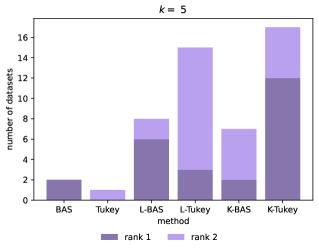
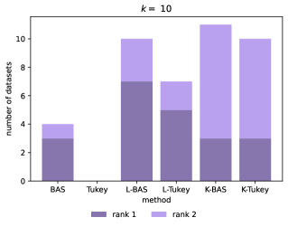
Figure 1: Plots of rank data for each private method.

4.3.1 Relative Performance

First, for each dataset and method, we compute the median $R^{2}$ of the final model across the 10 trials and then rank the methods, with the best method receiving a rank of 1. Figure 1 plots the number of times each method is ranked first or second.

At $k=5$ (left), $\mathsf{K}\text{-}\mathsf{Tukey}$ performs best by a significant margin: it ranks first on 48% of datasets, twice the fraction of any other method. It also ranks first or second on the largest fraction of datasets (68%). In some contrast, $\mathsf{L}\text{-}\mathsf{BAS}$ obtains the top ranking on 24% of datasets, whereas $\mathsf{K}\text{-}\mathsf{BAS}$ only does so on 8%; nonetheless, the two have nearly the same number of total first or second rankings. At $k=10$ (right), no clear winner emerges among the feature selecting methods, as $\mathsf{L}\text{-}\mathsf{BAS}$, $\mathsf{K}\text{-}\mathsf{BAS}$, and $\mathsf{K}\text{-}\mathsf{Tukey}$ are all first or second on around half the datasets, though the methods using $\mathsf{SubLasso}$ have a higher share of datasets ranked first.

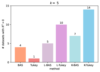
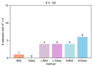
Figure 2: Plots of the number of datasets with positive $R^{2}$ for each private method.

4.3.2 Absolute Performance

Second, we count the number of datasets on which the method achieves a positive median $R^{2}$ (Figure 2), recalling that $R^{2}=0$ is achieved by the trivial model that always predicts the mean label. The $k=5$ (left) setting again demonstrates clear trends: $\mathsf{K}\text{-}\mathsf{Tukey}$ attains $R^{2}>0$ on 56% of datasets, $\mathsf{L}\text{-}\mathsf{Tukey}$ does so on 40%, $\mathsf{K}\text{-}\mathsf{BAS}$ does so on 28%, and $\mathsf{L}\text{-}\mathsf{BAS}$ on 20%. $\mathsf{DPKendall}$ therefore consistently demonstrates stronger performance than $\mathsf{SubLasso}$. As in the rank data, at $k=10$ the picture is less clear. However, $\mathsf{K}\text{-}\mathsf{Tukey}$ is still best by some margin, with the remaining feature selecting methods all performing roughly equally well.

4.4 Discussion

A few trends are apparent from Section 4.3. First, $\mathsf{DPKendall}$ generally achieves stronger final utility than $\mathsf{SubLasso}$, particularly for the Tukey mechanism; the effect is similar but smaller for $k=10$; and feature selection generally improves the performance of private linear regression.

Comparing Feature Selection Algorithms. A possible reason for $\mathsf{DPKendall}$’s improvement over $\mathsf{SubLasso}$ is that, while $\mathsf{SubLasso}$ takes advantage of the stability properties that Lasso exhibits in certain data regimes [21], this stability does not always hold in practice. Another possible explanation is that the feature coefficients passed to $\mathsf{Peel}$ scale with $O(n)$ for $\mathsf{DPKendall}$ and $m=O(\tfrac{n}{d})$ or $m=O(\tfrac{n}{k})$ for $\mathsf{SubLasso}$. Both algorithm’s invocations of $\mathsf{Peel}$ add noise scaling with $O(\tfrac{k}{\varepsilon})$, so $\mathsf{DPKendall}$’s larger scale makes it more robust to privacy-preserving noise. Finally, we emphasize that $\mathsf{DPKendall}$ achieves this even though its $O(dkn\log(n))$ runtime is asymptotically smaller than the $O(d^{2}n)$ runtime of $\mathsf{SubLasso}$ in most settings.

Choosing $\mathbf{k}$. Next, we examine the decrease in performance from $k=5$ to $k=10$. Conceptually, past a certain point adding marginally less informative features to a private model may worsen utility due to the privacy cost of considering these features. Moving from $k=5$ to $k=10$ may cross this threshold for many of our datasets; note from Figure 4 and Figure 5 in the Appendix that, of the 21 datasets used for $k=10$, 86% witness their highest private $R^{2}$ in the $k=5$ setting. Moreover, from $k=5$ to $k=10$ the total number of positive $R^{2}$ datasets across methods declines by more than 50%, from 41 to 19, with all methods achieving positive $R^{2}$ less frequently at $k=10$ than $k=5$. We therefore suggest $k=5$ as the more relevant setting, and a good choice in practice.

The Effect of Private Feature Selection. Much work aims to circumvent generic lower bounds for privately answering queries by taking advantage of instance-specific structure [6, 16, 33, 5]. Similar works exist for private optimization, either by explicitly incorporating problem information [35, 18] or showing that problem-agnostic algorithms can, under certain conditions, take advantage of problem structure organically [24]. We suggest that this paper makes a similar contribution: feature selection reduces the need for algorithms like Boosted AdaSSP and the Tukey mechanism to “waste” privacy on computations over irrelevant features. This enables them to apply less obscuring noise to the signal contained in the selected features. The result is the significant increase in utility shown here.

5 Conclusion

We briefly discuss a few of $\mathsf{DPKendall}$’s limitations. First, it requires an end user to choose the number of features $k$ to select. Second, $\mathsf{DPKendall}$’s use of Kendall rank correlation may struggle when ties are intrinsic to the data’s structure, e.g., when the data is categorical, as a monotonic relationship between feature and label becomes less applicable. Finally, Kendall rank correlation may fail to distinguish between a feature with a strong linear monotonic relationship with the label and a feature with a strong nonlinear monotonic relationship with the label, even though the former is more likely to be useful for linear regression. Unfortunately, it is not obvious how to incorporate relationships more sophisticated than simple monotonicity without sacrificing rank correlation’s low sensitivity. Answering these questions may be an interesting avenue for future work.

Nonetheless, the results of this paper demonstrate that $\mathsf{DPKendall}$ expands the applicability of plug-and-play private linear regression algorithms while providing more utility in less time than the current state of the art. We therefore suggest that $\mathsf{DPKendall}$ presents a step forward for practical private linear regression.

6 Alternative Notions of Correlation

6.1 Pearson

The Pearson correlation between some feature $X$ and the label $Y$ is defined by

$$r(X,Y)\coloneqq\frac{\mathsf{Cov}\left(X,Y\right)}{\sqrt{\mathsf{Var}\left(X\right)\mathsf{Var}\left(Y\right)}}.$$ (4)

Evaluated on a sample of $n$ points, this becomes

$$r(X,Y)\coloneqq\frac{\sum_{i=1}^{n}(X_{i}-\bar{X})(Y_{i}-\bar{Y})}{\sqrt{\sum_{i=1}^{n}(X_{i}-\bar{X})^{2}}\sqrt{\sum_{i=1}^{n}(Y_{i}-\bar{Y})^{2}}}.$$

where $\bar{X}$ and $\bar{Y}$ are sample means.

Lemma 6.1.

$r\in[-1,1]$.

Proof.

This is immediate from Cauchy-Schwarz. ∎

Note that a value of $-1$ is perfect anticorrelation and a value of $1$ is perfect correlation. A downside of Pearson correlation is that it is not robust. In particular, its sensitivity is the same as its range.

Lemma 6.2.

Pearson correlation has $\ell_{1}$-sensitivity $\Delta(r)=2$.

Proof.

Consider neighboring databases $D=\{(-1,-1),(1,1)\}$ and $D^{\prime}=\{(-1,-1),(1,1),(-c,c)\}$. $r(D)=1$, but

$$r(D^{\prime})= \ \frac{(-1+\tfrac{c}{3})(-1-\tfrac{c}{3})+(1+\tfrac{c}{3})(1-\tfrac{c}{3})+(-\frac{2c}{3}\cdot\tfrac{2c}{3})}{\sqrt{(-1+\tfrac{c}{3})^{2}+(1+\tfrac{c}{3})^{2}+(-\tfrac{2c}{3})^{2}}\sqrt{(-1-\tfrac{c}{3})^{2}+(1-\tfrac{c}{3})^{2}+(\tfrac{2c}{3})^{2}}}$$

$$\approx \ \frac{-(\tfrac{2c}{3})^{2}}{(\tfrac{2c}{3})^{2}}=-1$$

where the approximation is increasingly accurate as $c$ grows. ∎

6.2 Spearman

Spearman rank correlation is Pearson correlation applied to rank variables.

Definition 6.3.

Given data points $X_{1},\ldots,X_{n}\in\mathbb{R}$, the corresponding rank variables $R(X_{1}),\ldots,R(X_{n})$ are defined by setting $R(X_{i})$ to the position of $X_{i}$ when $X_{1},\ldots,X_{n}$ are sorted in descending order. Given data $(X,Y)$, the Spearman rank correlation is $\rho(X,Y)\coloneqq r(R(X),R(Y))$.

For example, given database $D=\{(0,1),(1,0),(2,3)\}$, its Spearman rank correlation is

$$\rho(D)\coloneqq r(\{(3,2),(2,3),(1,1)\}).$$

A useful privacy property of rank is that it does not depend on data scale. Moreover, if there are no ties then Spearman rank correlation admits a simple closed form.

Lemma 6.4.

$\rho(X,Y)=1-\frac{6\sum_{i=1}^{n}(R(X_{i})-R(Y_{i}))^{2}}{n(n^{2}-1)}$.

If we consider adding a “perfectly unsorted” data point with rank variables $(1,n+1)$ to a perfectly sorted database with rank variables $\{(1,1),(2,2),\ldots,(n,n)\}$, $\rho$ changes from 1 to $1-\frac{6(n+n^{2})}{n(n^{2}-1)}$. The sensitivity’s dependence on $n$ complicates its usage with add-remove privacy. Nonetheless, both Spearman and Kendall correlation’s use of rank makes them relatively easy to compute privately, and as the two methods are often used interchangeably in practice, we opt for Kendall rank correlation for simplicity.

7 Datasets

A summary of the datasets used in our experiments appears in Figure 3.

OpenML Task ID	n	d	$\lfloor n/d\rfloor$	$\lfloor n/5\rfloor$	$\lfloor n/10\rfloor$
361072	8192	22	372	1638	819
361073	15000	27	555	3000	1500
361074	16599	17	976	3319	1659
361075	7797	614	12	1559	779
361076	6497	12	541	1299	649
361077	13750	34	404	2750	1375
361078	20640	9	2293	4128	2064
361079	22784	17	1340	4556	2278
361085	10081	7	1440	2016	1008
361087	13932	14	995	2786	1393
361088	21263	80	265	4252	2126
361089	20640	9	2293	4128	2064
361091	515345	91	5663	103069	51534
361092	8885	83	107	1777	888
361093	4052	13	311	810	405
361094	8641	6	1440	1728	864
361095	166821	24	6950	33364	16682
361096	53940	27	1997	10788	5394
361098	10692	18	594	2138	1069
361099	17379	21	827	3475	1737
361100	39644	74	535	7928	3964
361101	581835	32	18182	116367	58183
361102	21613	20	1080	4322	2161
361103	394299	27	14603	78859	39429
361104	241600	16	15100	48320	24160

Figure 3: Parameters of the 25 datasets used in our experiments.

We briefly discuss the role of the intercept in these datasets. Throughout, we explicitly add an intercept feature (constant 1) to each vector. Where feature selection is applied, we explicitly remove the intercept feature during feature selection and then add it back to the $k$ selected features afterward. The resulting regression problem therefore has dimension $k+1$. We do this to avoid spending privacy budget selecting the intercept feature.

8 Modified PTR Lemma

This section describes a simple tightening of Lemma 3.6 from Amin et al. [2] (which is itself a small modification of Lemma 3.8 from Brown et al. [7]). $\mathsf{Tukey}$ uses the result as its propose-test-release (PTR) check, so tightening it makes the check easier to pass. Proving the result will require introducing details of the $\mathsf{Tukey}$ algorithm. The following exposition aims to keep this document both self-contained and brief; the interested reader should consult the expanded treatment given by Amin et al. [2] for further details.

Tukey depth was introduced by Tukey [32]. Amin et al. [2] used an approximation for efficiency. Roughly, Tukey depth is a notion of depth for a collection of points in space. (Exact) Tukey depth is evaluated over all possible directions in $\mathbb{R}^{d}$, while approximate Tukey depth is evaluated only over axis-aligned directions.

Definition 8.1 ([32, 2]).

A halfspace $h_{v}$ is defined by a vector $v\in\mathbb{R}^{d}$, $h_{v}=\{y\in\mathbb{R}^{d}\mid\langle v,y\rangle\geq 0\}$. Let $E=\{e_{1},...,e_{d}\}$ be the canonical basis for $\mathbb{R}^{d}$ and let $D\subset\mathbb{R}^{d}$. The approximate Tukey depth of a point $y\in\mathbb{R}^{d}$ with respect to $D$, denoted $\tilde{T}_{D}(y)$, is the minimum number of points in $D$ in any of the $2d$ halfspaces determined by $E$ containing $y$,

$$\tilde{T}_{D}(y)=\min_{v\in\pm E\text{ s.t. }y\in h_{v}}\sum_{x\in D}\mathbbm{1}_{x\in h_{v}}.$$

At a high level, Lemma 3.6 from Amin et al. [2] is a statement about the volumes of regions of different depths. The next step is to formally define these volumes.

Definition 8.2 ([2]).

Given database $D$, define $S_{i,D}=\{y\in\mathbb{R}^{d}\mid\tilde{T}_{D}(y)\geq i\}$ to be the set of points with approximate Tukey depth at least $i$ in $D$ and $V_{i,D}=\mathsf{vol}(S_{i,D})$ to be the volume of that set. When $D$ is clear from context, we write $S_{i}$ and $V_{i}$ for brevity. We also use $w_{D}(V_{d,D})\coloneqq\int_{S_{d,D}}\exp(\varepsilon\cdot\tilde{T}_{D}(y))dy$ to denote the weight assigned to $V_{d,D}$ by an exponential mechanism whose score function is $\tilde{T}_{D}$.

Amin et al. [2] define a family of mechanisms $A_{1},A_{2}$, …, where $A_{t}$ runs the exponential mechanism to choose a point of approximately maximal Tukey depth, but restricted to the domain of points with Tukey depth at least $t$. Since this domain is a data-dependent quantity, they use the PTR framework to select a safe depth $t$. We briefly recall the definitions of “safe” and “unsafe” databases given by Brown et al. [7], together with the key PTR result from Amin et al. [2].

Definition 8.3 (Definitions 2.1 and 3.1 [7]).

Two distributions $\mathcal{P},\mathcal{Q}$ over domain $\mathcal{W}$ are $(\varepsilon,\delta)$-indistinguishable, denoted $\mathcal{P}\approx_{\varepsilon,\delta}\mathcal{Q}$, if for any measurable subset $W\subset\mathcal{W}$,

$$\mathbb{P}_{w\sim\mathcal{P}}\left[w\in W\right]\leq e^{\varepsilon}\mathbb{P}_{w\sim\mathcal{Q}}\left[w\in W\right]+\delta\text{ and }\mathbb{P}_{w\sim\mathcal{Q}}\left[w\in W\right]\leq e^{\varepsilon}\mathbb{P}_{w\sim\mathcal{P}}\left[w\in W\right]+\delta.$$

Database $D$ is $(\varepsilon,\delta,t)$-safe if for all neighboring $D^{\prime}\sim D$, we have $A_{t}(D)\approx_{\varepsilon,\delta}A_{t}(D^{\prime})$. Let $\mathtt{Safe}_{(\varepsilon,\delta,t)}$ be the set of safe databases, and let $\mathtt{Unsafe}_{(\varepsilon,\delta,t)}$ be its complement.

We can now restate Lemma 3.6 from Amin et al. [2]. Informally, it states that if the volume of an “outer” region of Tukey depth is not much larger than the volume of an “inner” region, the difference in depth between the two is a lower bound on the distance to an unsafe database. For the purpose of this paper, $\mathsf{Tukey}$ applies this result by finding such a $k$, adding noise for privacy, and checking that the resulting distance to unsafety is large enough that subsequent steps will be privacy-safe.

Lemma 8.4.

Define $M(D)$ to be a mechanism that receives as input database $D$ and computes the largest $k\in\{0,\ldots,t-1\}$ such that there exists $g>0$ where

$$\frac{V_{t-k-1,D}}{V_{t+k+g+1,D}}\cdot e^{-\varepsilon g/2}\leq\delta$$

or outputs $-1$ if the inequality does not hold for any such $k$. Then for arbitrary $D$

1. $M$ is 1-sensitive, and

2. for all $z\in\mathtt{Unsafe}_{(\varepsilon,4e^{\varepsilon}\delta,t)}$, $d_{H}(D,z)>M(D)$.

We provide a drop-in replacement for Lemma 8.4 that slightly weakens the requirement placed on $k$.

Lemma 8.5.

Define $M(D)$ to be a mechanism that receives as input database $D$ and computes the largest $k\in\{0,\ldots,t-1\}$ such that

$$\frac{V_{t-k-1,D}}{w_{D}(V_{t+k-1,D})}\cdot e^{\varepsilon(t+k+1)}\leq\delta$$

or outputs $-1$ if the inequality does not hold for any such $k$. Then for arbitrary $D$

1. $M$ is 1-sensitive, and

2. for all $z\in\mathtt{Unsafe}_{(\varepsilon,4e^{\varepsilon}\delta,t)}$, $d_{H}(D,z)>M(D)$.

The new result therefore replaces the denominator $V_{t+k+g+1,D}\cdot e^{\varepsilon g/2}$ with denominator $\frac{w_{D}(V_{t+k-1,D})}{e^{\varepsilon(t+k+1)}}$. Every point in $V_{t+k-1,D}$ of depth at least $t+k+g+1$ has score at least $t+k+g+1$, so $\frac{w_{D}(V_{t+k-1,D})}{e^{\varepsilon(t+k+1)}}\geq V_{t+k+g+1,D}\cdot e^{\varepsilon g}$, so $V_{t+k+g+1,D}\cdot e^{\varepsilon g/2}\leq\frac{w_{D}(V_{t+k+g+1,D})}{e^{\varepsilon(t+k+1)}}$ and the check for the new result is no harder to pass. To see that it may be easier, note that only the new result takes advantage of the higher scores of deeper points in $V_{t+k-1,D}$.

Proof of Lemma 8.5.

First we prove item 1. Let $D$ and $D^{\prime}$ be any neighboring databases and suppose WLOG that $D^{\prime}=D\cup\{x\}$. We want to show that $|M(D)-M(D^{\prime})|\leq 1$.

First we prove relationships between the points with approximate Tukey depth at least $p$ and $p-1$ in datasets $D$ and $D^{\prime}$. From the definition of approximate Tukey depth, together with the fact that $D^{\prime}$ contains one additional point, for any point $y$, we are guaranteed that $\tilde{T}_{D}(y)\leq\tilde{T}_{D^{\prime}}(y)\leq\tilde{T}_{D}(y)+1$. Recall that $S_{p,D}$ is the set of points with approximate Tukey depth at least $p$ in $D$. This implies that $S_{p+1,D}\subset S_{p,D}$. Next, since for every point $y$ we have $\tilde{T}_{D^{\prime}}(y)\geq\tilde{T}_{D}(y)$, we have that $S_{p,D}\subset S_{p,D^{\prime}}$. Finally, since $\tilde{T}_{D}(y)\geq\tilde{T}_{D^{\prime}}(y)-1$, we have that $S_{p,D^{\prime}}\subset S_{p-1,D}$. Taken together, we have

$$S_{p+1,D}\subset S_{p,D}\subset S_{p,D^{\prime}}\subset S_{p-1,D}.$$

It follows that

$$V_{p+1,D}\leq V_{p,D}\leq V_{p,D^{\prime}}\leq V_{p-1,D}.$$ (5)

Next, since the unnormalized exponential mechanism density $y\mapsto\exp(y\hat{T}_{D}(y))$ is non-negative, we have that $w_{D}(V_{p+1,D})=\int_{S_{p+1,D}}\exp(\epsilon\tilde{T}_{D}(y))\,dy\leq\int_{S_{p,D}}\exp(\epsilon\tilde{T}_{D}(y))\,dy=w_{D}(V_{p,D})$. Using the fact that $\tilde{T}_{D}(y)\leq\tilde{T}_{D^{\prime}}(y)$, we have that $w_{D}(V_{p,D})=\int_{S_{p,D}}\exp(\epsilon\tilde{T}_{D}(y))\,dy\leq\int_{S_{p,D^{\prime}}}\exp(\epsilon\tilde{T}_{D^{\prime}}(y))\,dy=w_{D^{\prime}}(V_{p,D^{\prime}})$. Finally, using the fact that $\tilde{T}_{D^{\prime}}(y)\leq\tilde{T}_{D}(y)+1$, we have $w_{D^{\prime}}(V_{p,D^{\prime}})=\int_{S_{p,D^{\prime}}}\exp(\varepsilon\tilde{T}_{D^{\prime}}(y))\,dy\leq\int_{S_{p-1,D}}\exp(\epsilon\tilde{T}_{D}(y)+\epsilon)\,dy=e^{\epsilon}w_{D}(V_{p-1,D})$. Together, this gives

$$w_{D}(V_{p+1,D})\leq w_{D}(V_{p,D})\leq w_{D^{\prime}}(V_{p,D^{\prime}})\leq w_{D}(V_{p-1,D})\cdot e^{\varepsilon}.$$ (6)

Now suppose there exists $k^{*}_{D^{\prime}}\geq 0$ such that $\tfrac{V_{t-k^{*}_{D^{\prime}}-1,D^{\prime}}}{w_{D^{\prime}}(V_{t+k^{*}_{D^{\prime}}+2,D^{\prime}})}\cdot e^{\varepsilon(t+k^{*}_{D^{\prime}}+1)}\leq\delta$. Then by Equation 5, $V_{t-k^{*}_{D^{\prime}}-1,D^{\prime}}\geq V_{t-k^{*}_{D^{\prime}},D}$, and by Equation 6 $w_{D^{\prime}}(V_{t+k^{*}_{D^{\prime}}+2,D^{\prime}})\leq w_{D}(V_{t+k^{*}_{D^{\prime}}+1,D})\cdot e^{\varepsilon}$, so $\tfrac{V_{t-k^{*}_{D^{\prime}},D}}{w_{D}(V_{t+k^{*}_{D^{\prime}}+1,D})}\cdot e^{\varepsilon(t+k^{*}_{D^{\prime}})}\leq\delta$ and then $k^{*}_{D}\geq k^{*}_{D^{\prime}}-1$. Similarly, if there exists $k^{*}_{D}\geq 0$ such that $\tfrac{V_{t-k^{*}_{D}-1,D}}{w_{D}(V_{t+k^{*}_{D}+2,D)}}\cdot e^{\varepsilon(t+k^{*}_{D}+1)}\leq\delta$, then by Equation 5 $V_{t-k^{*}_{D}-1,D}\geq V_{t-k^{*}_{D},D^{\prime}}$, and by Equation 6 $w_{D}(V_{t+k^{*}_{D}+2,D})\leq w_{D^{\prime}}(V_{t+k^{*}_{D}+2,D^{\prime}})$, so $\tfrac{V_{t-k^{*}_{D},D^{\prime}})}{w_{D^{\prime}}(V_{t+k^{*}_{x}+2,D^{\prime}})}\cdot e^{\varepsilon(t+k^{*}_{D^{\prime}})}\leq\delta$, and $k^{*}_{D^{\prime}}\geq k^{*}_{D}-1$. Thus if $k^{*}_{D}\geq 0$ or $k^{*}_{D^{\prime}}\geq 0$, $|k^{*}_{D}-k^{*}_{D^{\prime}}|\leq 1$. The result then follows since $k^{*}\geq-1$.

As in Lemma 8.4, item 2 is a consequence of Lemma 3.8 from Brown et al. [7] and the fact that $k^{*}=-1$ is a trivial lower bound on distance. The only change made to the proof of Lemma 3.8 of Brown et al. [7] is, in its notation, to replace its denominator lower bound with

$$w_{z}(V_{t-1,z})\geq w_{x}(V_{t+k-1,x})\cdot e^{-k\varepsilon}$$

This uses the fact that $x$ and $z$ differ in at most the addition or removal of $k$ data points. Thus $V_{t+k-1,x}\leq V_{t-1,z}$, and no point’s score increases by more than $k$ from $V_{t-1,z}$ to $V_{t+k-1,x}$. Since their numerator upper bound is $V_{t-k-1,x}\cdot e^{\varepsilon(t+1)}$ (note that the 2 is dropped here because approximate Tukey depth is monotonic; see Section 7.3 of [2] for details), the result follows. ∎

9 Extended Experiment Results

Task ID	$\mathsf{NonDP}$	$\mathsf{BAS}$	$\mathsf{Tukey}$	$\mathsf{L}\text{-}\mathsf{BAS}$	$\mathsf{L}\text{-}\mathsf{Tukey}$	$\mathsf{K}\text{-}\mathsf{BAS}$	$\mathsf{K}\text{-}\mathsf{Tukey}$
361072	7.3e-01	7.8e-01	$-\infty$	-2.7e-02	1.0e-01	2.1e-01	1.0e-01
361073	4.6e-01	-3.4e+00	$-\infty$	-4.6e-01	-2.3e-02	-4.8e-01	-4.3e-01
361074	8.0e-01	-4.5e+04	-6.6e+02	-8.2e+02	-1.7e+02	-5.6e+05	3.1e-01
361075	6.2e-01	-3.6e+02	$-\infty$	3.2e-03	2.2e-02	5.2e-03	7.1e-02
361076	2.8e-01	-3.4e+00	$-\infty$	-5.6e-01	-2.5e-01	-4.3e+00	8.5e-02
361077	8.2e-01	-2.1e+08	$-\infty$	-1.0e+07	3.7e-01	-1.9e+08	6.6e-01
361078	6.5e-01	-1.1e+03	-6.4e+00	-7.4e-01	-1.2e+00	-6.1e+02	-9.5e-01
361079	2.6e-01	-5.4e+00	-1.0e+01	-1.3e+01	-2.e+00	-9.4e+00	-6.8e-01
361085	3.3e-01	-2.e+01	3.3e-01	-1.7e+01	2.8e-01	-1.3e+01	3.7e-01
361087	7.2e-01	-3.1e+03	-8.8e+04	-4.7e+00	-1.9e+02	-2.8e+00	6.6e-01
361088	7.3e-01	5.4e-02	$-\infty$	1.4e-01	3.e-01	2.1e-01	3.6e-01
361089	6.2e-01	-3.e+00	-1.5e+01	-1.3e+00	-5.9e+00	-5.9e+04	-2.6e-01
361091	2.4e-01	-3.0e+04	-1.9e+00	-3.0e+04	3.8e-02	-3.1e+04	4.9e-02
361092	2.0e-02	-4.7e+05	$-\infty$	-4.1e+04	-1.4e+08	-1.3e+05	-9.3e+08
361093	4.3e-01	-5.6e-02	$-\infty$	-4.6e-02	$-\infty$	-4.9e-02	$-\infty$
361094	8.3e-01	4.2e-01	-3.8e+05	-1.0e+00	-4.2e+05	-2.4e+00	-3.0e+05
361095	2.2e-01	-1.0e+00	-1.2e+09	-8.0e-01	2.e-01	1.5e-01	2.1e-01
361096	9.7e-01	-9.1e+02	-1.e+08	-4.9e+00	9.1e-01	7.1e-01	8.8e-01
361098	8.6e-01	-2.9e+01	$-\infty$	-3.9e+00	-3.1e+00	-2.2e-01	-5.6e+00
361099	4.0e-01	-4.4e-01	-4.8e+10	-4.8e-01	-9.8e-03	-4.2e-01	3.2e-01
361100	1.2e-01	-6.3e+01	$-\infty$	-1.1e+00	-2.8e-02	-4.6e-01	-1.7e-01
361101	3.3e-01	-9.3e+01	-5.9e+08	3.6e-01	2.e-01	3.0e-01	2.1e-01
361102	7.6e-01	-4.1e+02	-1.4e+15	6.8e-02	-2.6e-01	-4.0e+00	-5.3e+00
361103	5.3e-01	4.3e-01	-6.3e+07	5.e-01	4.9e-01	3.3e-01	4.8e-01
361104	6.8e-01	-3.7e+03	-6.4e+07	-1.5e+02	-2.6e+05	-8.3e-01	-2.9e+01

Figure 4: $R^{2}$ values for $k=5$. Each entry is the median test value from 10 trials. The top two private values for each dataset are bolded.

Task ID	$\mathsf{NonDP}$	$\mathsf{BAS}$	$\mathsf{Tukey}$	$\mathsf{L}\text{-}\mathsf{BAS}$	$\mathsf{L}\text{-}\mathsf{Tukey}$	$\mathsf{K}\text{-}\mathsf{BAS}$	$\mathsf{K}\text{-}\mathsf{Tukey}$
361072	7.4e-01	5.3e-01	$-\infty$	3.5e-01	1.8e-01	7.3e-01	8.2e-02
361073	4.6e-01	-8.2e-01	$-\infty$	-4.4e-01	-1.7e+00	-4.8e-01	-1.6e+01
361074	8.1e-01	-2.3e+06	-1.3e+03	-5.6e+06	-3.4e+02	-7.2e+04	-1.4e+02
361075	6.2e-01	-1.7e+02	$-\infty$	7.5e-02	-9.7e-01	3.1e-02	-2.8e+00
361076	2.8e-01	-2.4e+02	-8.2e+04	-2.7e+01	-3.5e+03	-2.4e+01	-1.4e+03
361077	7.9e-01	-1.1e+08	$-\infty$	-1.4e+07	-3.1e+01	-2.1e+08	-1.7e+02
361079	2.4e-01	-1.8e+00	-3.7e+01	-1.2e+01	-8.1e-01	-4.1e+00	-1.5e+00
361087	7.1e-01	-3.7e+01	-1.5e+04	-7.2e+00	-4.8e+03	-8.5e+01	-2.e+01
361088	7.3e-01	-1.9e+00	$-\infty$	1.2e-01	9.2e-02	1.2e-01	7.1e-02
361091	2.4e-01	-3.0e+04	-3.4e+00	-3.0e+04	6.8e-02	-3.1e+04	5.7e-02
361092	4.0e-02	-2.4e+06	$-\infty$	-8.7e+05	-7.6e+09	-7.5e+05	-3.7e+10
361093	4.3e-01	-3.2e-02	$-\infty$	-5.e-01	$-\infty$	-1.1e-01	$-\infty$
361095	2.2e-01	-1.9e+01	-1.2e+09	-8.6e-01	-2.4e+07	-1.4e+00	2.1e-01
361096	9.8e-01	-3.7e+02	-1.0e+08	-3.4e+03	-1.8e+00	-1.0e+03	4.2e-01
361098	8.6e-01	-1.8e+02	$-\infty$	-4.1e-01	-1.3e+07	-9.5e-01	-5.8e-01
361099	4.0e-01	-4.3e-01	-2.3e+10	-4.9e-01	-2.4e+09	-4.8e-01	-2.5e+08
361100	1.2e-01	-9.2e+01	$-\infty$	-1.6e+00	-8.2e-02	-3.5e+00	-5.2e-01
361101	3.4e-01	-3.3e+03	-1.7e+08	-8.1e-01	-1.4e+02	-9.5e-01	-4.7e+05
361102	7.5e-01	-9.5e+02	-1.7e+15	-1.3e+00	-1.5e+15	-2.5e+01	-1.4e+05
361103	5.4e-01	-2.6e+00	-1.2e+08	4.9e-01	5.1e-01	3.5e-01	4.9e-01
361104	6.8e-01	-9.e+02	-1.0e+08	-2.9e+03	-3.5e+07	-1.4e+03	-6.6e+05

Figure 5: This figure records the same information as Figure 4, but for $k=10$.

References

- Amin et al. [2019] Kareem Amin, Travis Dick, Alex Kulesza, Andres Munoz Medina, and Sergei Vassilvitskii. Differentially private covariance estimation. Neural Information Processing Systems (NeurIPS), 2019.
- Amin et al. [2023] Kareem Amin, Matthew Joseph, Mónica Ribero, and Sergei Vassilvitskii. Easy differentially private linear regression. In International Conference on Learning Representations (ICLR), 2023.
- Anzarmou et al. [2022] Youssef Anzarmou, Abdallah Mkhadri, and Karim Oualkacha. The Kendall interaction filter for variable interaction screening in high dimensional classification problems. Journal of Applied Statistics, 2022.
- Bhaskar et al. [2010] Raghav Bhaskar, Srivatsan Laxman, Adam Smith, and Abhradeep Thakurta. Discovering frequent patterns in sensitive data. In Knowledge Discovery and Data Mining (KDD), 2010.
- Błasiok et al. [2019] Jaroslaw Błasiok, Mark Bun, Aleksandar Nikolov, and Thomas Steinke. Towards instance-optimal private query release. In Symposium on Discrete Algorithms (SODA), 2019.
- Blum et al. [2008] Avrim Blum, Katrina Ligett, and Aaron Roth. A learning theory approach to non-interactive database privacy. In Symposium on the Theory of Computing (STOC), 2008.
- Brown et al. [2021] Gavin Brown, Marco Gaboardi, Adam Smith, Jonathan Ullman, and Lydia Zakynthinou. Covariance-Aware Private Mean Estimation Without Private Covariance Estimation. In Neural Information Processing Systems (NeurIPS), 2021.
- Chaudhuri et al. [2012] Kamalika Chaudhuri, Anand Sarwate, and Kaushik Sinha. Near-optimal differentially private principal components. Neural Information Processing Systems (NIPS), 2012.
- Durfee and Rogers [2019] David Durfee and Ryan M Rogers. Practical differentially private top-k selection with pay-what-you-get composition. Neural Information Processing Systems (NeurIPS), 2019.
- Dwork et al. [2006] Cynthia Dwork, Frank McSherry, Kobbi Nissim, and Adam Smith. Calibrating noise to sensitivity in private data analysis. In Theory of Cryptography Conference (TCC), 2006.
- Dwork et al. [2014] Cynthia Dwork, Kunal Talwar, Abhradeep Thakurta, and Li Zhang. Analyze gauss: optimal bounds for privacy-preserving principal component analysis. In Symposium on Theory of Computing (STOC), 2014.
- Efron et al. [2004] Bradley Efron, Trevor Hastie, Iain Johnstone, and Robert Tibshirani. Least angle regression. Annals of Statistics, 2004.
- Gillenwater et al. [2022] Jennifer Gillenwater, Matthew Joseph, Andres Munoz Medina, and Monica Ribero Diaz. A Joint Exponential Mechanism For Differentially Private Top-. In International Conference on Machine Learning (ICML), 2022.
- Google [2023] Google. private_kendall. https://github.com/google-research/google-research/tree/master/private_kendall, 2023.
- Hardt and Roth [2012] Moritz Hardt and Aaron Roth. Beating randomized response on incoherent matrices. In Symposium on Theory of Computing (ICML), 2012.
- Hardt and Rothblum [2010] Moritz Hardt and Guy N Rothblum. A multiplicative weights mechanism for privacy-preserving data analysis. In Foundations of Computer Science (FOCS), 2010.
- Jain and Thakurta [2014] Prateek Jain and Abhradeep Guha Thakurta. (Near) dimension independent risk bounds for differentially private learning. In International Conference on Machine Learning (ICML), 2014.
- Kairouz et al. [2021] Peter Kairouz, Monica Ribero Diaz, Keith Rush, and Abhradeep Thakurta. (Nearly) Dimension Independent Private ERM with AdaGrad Rates via Publicly Estimated Subspaces. In Conference on Learning Theory (COLT), 2021.
- Kapralov and Talwar [2013] Michael Kapralov and Kunal Talwar. On differentially private low rank approximation. In Symposium on Discrete Algorithms (SODA), 2013.
- Kendall [1938] Maurice G Kendall. A new measure of rank correlation. Biometrika, 1938.
- Kifer et al. [2012] Daniel Kifer, Adam Smith, and Abhradeep Thakurta. Private convex empirical risk minimization and high-dimensional regression. In Conference on Learning Theory (COLT), 2012.
- Knight [1966] William R Knight. A computer method for calculating Kendall’s tau with ungrouped data. Journal of the American Statistical Association, 1966.
- Kusner et al. [2016] Matt J Kusner, Yu Sun, Karthik Sridharan, and Kilian Q Weinberger. Private causal inference. In Artificial Intelligence and Statistics (AISTATS), 2016.
- Li et al. [2022] Xuechen Li, Daogao Liu, Tatsunori B Hashimoto, Huseyin A Inan, Janardhan Kulkarni, Yin-Tat Lee, and Abhradeep Guha Thakurta. When Does Differentially Private Learning Not Suffer in High Dimensions? Neural Information Processing Systems (NeurIPS), 2022.
- McSherry and Mironov [2009] Frank McSherry and Ilya Mironov. Differentially private recommender systems: Building privacy into the netflix prize contenders. In Knowledge Discovery and Data Mining (KDD), 2009.
- Owen [1980] Donald Bruce Owen. A table of normal integrals. Communications in Statistics-Simulation and Computation, 1980.
- Sarathy et al. [2023] Jayshree Sarathy, Sophia Song, Audrey Emma Haque, Tania Schlatter, and Salil Vadhan. Don’t look at the data! How differential privacy reconfigures data subjects, data analysts, and the practices of data science. In Conference on Human Factors in Computing Systems (CHI), 2023.
- Stoddard et al. [2014] Ben Stoddard, Yan Chen, and Ashwin Machanavajjhala. Differentially private algorithms for empirical machine learning. arXiv preprint arXiv:1411.5428, 2014.
- Talwar et al. [2015] Kunal Talwar, Abhradeep Guha Thakurta, and Li Zhang. Nearly optimal private lasso. Neural Information Processing Systems (NIPS), 2015.
- Tang et al. [2023] Shuai Tang, Sergul Aydore, Michael Kearns, Saeyoung Rho, Aaron Roth, Yichen Wang, Yu-Xiang Wang, and Zhiwei Steven Wu. Improved Differentially Private Regression via Gradient Boosting. arXiv preprint arXiv:2303.03451, 2023.
- Thakurta and Smith [2013] Abhradeep Guha Thakurta and Adam Smith. Differentially private feature selection via stability arguments, and the robustness of the lasso. In Conference on Learning Theory (COLT), 2013.
- Tukey [1975] John W Tukey. Mathematics and the picturing of data. In International Congress of Mathematicians (IMC), 1975.
- Ullman [2015] Jonathan Ullman. Private multiplicative weights beyond linear queries. In Principles of Database Systems (PODS), 2015.
- Wang [2018] Yu-Xiang Wang. Revisiting differentially private linear regression: optimal and adaptive prediction & estimation in unbounded domain. In Uncertainty in Artificial Intelligence (UAI), 2018.
- Zhou et al. [2021] Yingxue Zhou, Zhiwei Steven Wu, and Arindam Banerjee. Bypassing the ambient dimension: Private sgd with gradient subspace identification. International Conference on Learning Representations (ICLR), 2021.