Dynamical correlations in simple disorder and complex disorder liquids

Abstract

Liquids in equilibrium exhibit two types of disorder, simple and complex. Typical simple disorder liquid are liquid nitrogen, or weakly polar liquids. Complex liquids concern those who can form long lived local assemblies, and cover a large range from water to soft matter and biological liquids. The existence of such structures leaves characteric features upon the atom-atom correlation functions, concerning both atoms which directly participate to these structure and those who do not. The question we ask here is: does these features have also characteristic dynamical aspects, which could be tracked through dynamical correlation functions. Herein, we compare the van Hove function, intermediate scattering function and the dynamical structure factor, for both types of liquids, using force field models and computer simulations. The calculations reveal the paradoxical fact that neighbouring atom correlations for simple disorder liquids relax slower than that for complex disorder liquids, while prepeak features typical of complex disorder liquids relax even slower. This is an indication of the existence of fast kinetic self-assembly processes in complex disorder liquids, while the lifetime of such assemblies itself is quite slow. This is further confirmed by the existence of a very low-$k$ dynamical pre-peak uncovered in the case of water and ethanol.

^†Laboratoire de Physique Théorique de la Matière Condensée (UMR CNRS 7600), Sorbonne Université, 4 Place Jussieu, F75252, Paris cedex 05, France.

^‡Department of Physics, Faculty of Science, University of Split, Ruđera Boškovića 33, 21000, Split, Croatia.

^∤ Laboratoire de Traitement et Communication de l’Information, Telecom Paris, Institut Polytechnique de Paris, 19, place Marguerite Perey CS 20031 F-91123 Palaiseau, France.

1 Introduction

While liquids are known to be the archetype of disorder (excluding all liquid crystalline materials), liquid nitrogen and water belong to two different classes of liquids [1, 2]. The first one is characterised by simple disorder, while the second is about complex disorder, due to the presence of hydrogen connectivity [3, 4], which gives a local coherence that simple disorder liquids do not have. Other complex disorder liquids, such as alcohols, show chain like clustering of the hydroxyl head groups [5, 6, 7, 8, 9, 10]. These are elementary forms of self-assembly, which is the major property of more complex liquids, such as soft matter [11, 12, 13] or biological liquids [14]. Admittedly, disorder is not really a physical chemistry property, such as energy or entropy. However, it is related to the structural properties, which are a window into the microscopic arrangement of particles, from statistical point of view. In that, it is much more specific of the nature of liquids than properties like energy or entropy.

Perhaps the typical experimental evidence of such complex form of disorder is the radiation scattering pre-peak [5, 6, 15, 16, 17, 18, 19, 8, 20] in the scattering intensity $I(k)$, which witnesses the existence of local aggregates. For typical liquids of small molecules, the relevant experiment is wide angle x-ray scattering, which covers the range from $k=0$ until the atom-atom peak which about $k\approx 1.5-2\mathring{A}^{-1}$. Interestingly, not all complex disorder systems have a radiation scattering pre-peak [21, 22, 23, 24]. This is because the scattering pre-peak is the result of sum of pre-peaks and anti-peaks in specific atom-atom structure factors [24, 25], which sometimes tend to exactly cancel each other, thus leaving a net small-$k$ raise in $I(k)$, which is interpreted as the presence of large heterogeneity [26].

$I(k)$ is however a static indicator, and it would be interesting to have information about the kinetics and lifetime of the local heterogeneity and labile structures, and also how they affect various dynamical quantities. Unfortunately, there is no such thing as time dependent radiation scattering intensity $I(k,t)$ for x-ray scattering. Spectroscopy methods provide informations about the molecular relaxation, but these mostly focus on intra-molecular relaxation, and the coupling with inter-molecular relaxation must be obtained through interpretations.

Computer simulation techniques can provide a direct access to atom-atom dynamical pair correlation functions and the corresponding structure factors. However, this implies a necessary model dependence, which can be a drawback in some cases, such as that of mixtures involving aggregate forming components, as exemplified with the difficulties in computing the Kirkwood-Buff integrals [27, 28, 29, 30, 31, 32, 33]. Despite these difficulties, it is interesting to obtain dynamical correlation functions, since these could provide a good idea of the molecular kinetics, as well an opportunity to check agreements with dynamical quantities, such as transport coefficients for example.

In the present work, we compute atom-atom van Hove functions $G(r,t)$, corresponding intermediate scattering functions $F(k,t)$ and dynamical structure factors $S(k,\omega)$, hence covering the direct and reciprocal spaces, as well time and frequency domains, and for various types of single component liquids, both of simple and complex disorder types. The liquids studied herein are carbon-tetrachloride, acetone, water and ethanol. In addition to allowing us to find correspondances between typical structural features associated with local clustering in various representation of correlations, we expect to learn correspondence between the relaxation mechanisms themselves, since these functions are microscopic probes of better investigation power than $I(k,t)$ could access.

There has been previous report of dynamical correlations in the literature, which we briefly review here. It is interesting to note that not, compared to calculation from computer of static correlations covering many types of liquids, there are remarkably much less coverage with dynamical ones. Early calculations concern mostly simple liquids, and lately water, but in the supercooled regime. Going into details, dynamical structure factors have been calculated for liquid metals, such as rubidium [34, 35] and aluminum [36, 37], and molten salts [38]. Similar analysis have been performed for polyisoprene and their MD simulations gave a clearer interpretation of the experimentally observed results [39]. Models for glass forming systems, like silica, were studied via MD simulations by Sciortino et al. [40] and for liquid iron by Wu et al. [41]. Dynamical correlations have lately been reported from inelastic x-ray scattering for liquid water at ambient conditions and inelastic neutron scattering at various temperatures [42]. MD results of the coherent dynamic structure factor of liquid water at the mesoscale have been presented by Alvarez et al. [43].

In view of this scarcity of coverage, the present study could, although focused on the quality of disorder, could be equally seen as providing the missing coverage other types of liquids than those studied so far.

The remainder of the manuscript is as follows. We first recall what dynamical atom-atom correlations are, and how they are interrelated. We then explain how they are calculated and the models and simulation details. Then, in the results section, we study into some detail these correlation functions and investigate what they can tell us about the molecular relaxations at different levels. A final section gathers what perspectives this study inspires and outlines our conclusions.

2 Atom-atom dynamical correlations

We make the choice of dealing with atom-atom correlation functions, even in the case of molecular liquids, instead of orientational correlation functions. It is generally believed that these latter functions are a better choice, since they contain information irretrievably lost in the former [44]. In addition, atom-atom correlation functions can be obtained from the orientational ones, but not the opposite [45]. However, these orientation correlations cannot be manipulated directly and necessitate and infinite number of terms in the standard rotational invariant expansion [46]. For instance, the atom-atom functions can be obtained only as a sum of such infinite number of terms [47]. This raises practical issues about the convergence, which can become crucial when specific orientations play an important, such as the hydrogen bond, for instance. Since atom-atom correlation functions contain both the intra-molecular and inter-molecular correlations, we believe that these are much simpler functions to calculate, and they always come in a finite number, even when large proteins are concerned. There are additional two appealing reasons for using atom-atom functions. Firstly, they implicitly assume that molecular liquids are like a “soup of atoms”, some of which are grouped through intra-molecular correlations, hence making a link between covalent binding and labile binding, with open interesting possibilities to unify both representations into a single one. Secondly, as shown below in this Section, the intra-molecular part is in fact very naturally connected to the self part of the van Hove function, thus becoming a necessary ingredient in a dynamical approach of molecular liquids,of which the static representation is only the $t=0$ limit. We believe that these 2 reasons enforce an overwhelming bias in choosing atom-atom correlations over orientational ones.

For the above mentioned reasons, we dwell into details of these dynamical functions from the atomic perspective, even though many of these details can be found in most text books [47, 48].

2.1 The van Hove function

The time dependent microscopic density per particle of atomic species $a$ , at position $\mathbf{r}$ and time $t$, is defined as:

$$\rho_{i;a}(\mathbf{r},t)=\delta\left[\mathbf{r}-\mathbf{r}_{i;a}(t)\right]$$ (1)

where $\mathbf{r}_{i;a}(t)$ is the time dependent position of particle $i$ or atomic species $a$, in the lab fixed frame. This definition holds regardless whether the atom belongs to a molecule or not, since we use the “molecular liquid=soup of atoms” convention, where each atomic species is named differently, even if it concerns the same atom type. In this convention, the two hydrogen atoms of water are labeled differently (e.g $H_{1}$ and $H_{2}$, for instance). From this per-particle microscopic density, one defines the microscopic random variable which is the total density of atomic species $a$ by summing over all atom $i$ of species $a$:

$$\rho_{a}(\mathbf{r},t)=\sum_{i}\rho_{i;a}(\mathbf{r},t)$$ (2)

From these two random variables, one can compute various type of statistical averages in selected statistical ensembles. For instance, in the constant $NVT$ Canonical ensemble, the simple 1-body average give the trivial relation:

$$<\rho_{a}(\mathbf{r},t)>=\frac{N_{a}}{V}=\rho_{a}$$ (3)

where $N_{a}$ is the number of atoms of species a in the volume V, $\rho_{a}$the number density of species a, and we have used the fact that we consider liquids at equilibrium which are homogeneous and isotropic. In the “molecular liquid=soup of atoms” convention, for given molecular species $m$ , since all atoms are uniquely represented, the number density $\rho_{a_{m}}$ of any atomic species $a_{m}$ within that molecule is exactly that $\rho_{m}$ of the molecular species itself $\rho_{a}=\rho_{m}$. For this reason, we will use $\rho_{a}$without any ambiguity about its meaning.

Two body correlations can be defined in a similar way, such as $\rho_{ab}^{(2)}(\mathbf{r}_{1},\mathbf{r}_{2},t)=<\rho_{a}(\mathbf{r}_{1},t)\rho_{b}(\mathbf{r}_{2},0)>$ which correlates two types of atoms $a$ and $b$ at respective positions $\mathbf{r}_{1}$ and $\mathbf{r}_{2},$and taken at two different times, where we set arbitrarily the origin of time the system of atomic species $b$. Using the fact that one can use the variable change $(\mathbf{r},\mathbf{r}^{\prime})\rightarrow(\mathbf{r},\mathbf{R})$, where $\mathbf{r}=\mathbf{r}_{1}-\mathbf{r}_{2}$ and $\mathbf{R}=(\mathbf{r}_{1}+\mathbf{r}_{2})/2,$whose Jacobian is $1$, using the random variable in Eq.(1) we define the dimensionless self van Hove function for homogeneous and isotropic liquids as:

$$G_{aa}^{(s)}(r,t)=\frac{1}{\rho_{a}^{2}V}\sum_{i}\int d\hat{\mathbf{r}}\int d\mathbf{R}<\rho_{i;a}(\mathbf{r}_{1},t)\rho_{i;a}(\mathbf{r}_{2},0)>$$ (4)

where we have integrated both on the irrelevant $\mathbf{R}$ variable, as well as the unit vector $\hat{\mathbf{r}}$ representing the orientational part of $\hat{\mathbf{r}}$ of $\mathbf{r}$, since the system is isotropic and the pair correlation function depends only on $r=|\mathbf{r}|=|\mathbf{r}_{1}-\mathbf{r}_{2}|$ .

Similarly, using the total microscopic density defined in Eq.(2), we define the dimensionless total van Hove function as:

$$G_{ab}(r,t)=\frac{1}{\rho_{a}\rho_{b}V}\int d\hat{\mathbf{r}}\int d\mathbf{R}<\rho_{a}(\mathbf{r}_{1},t)\rho_{b}(\mathbf{r}_{2},0)>$$ (5)

Using Eq.(2), this latter equation can be split into two parts, a distinct van Hove correlation function

$$G_{ab}^{(d)}(r,t)=\frac{1}{\rho_{a}\rho_{b}V}\int d\hat{\mathbf{r}}\sum_{i\neq j}\int d\mathbf{R}<\rho_{i;a}(\mathbf{r}_{1},t)\rho_{j;b}(\mathbf{r}_{2},0)>$$ (6)

and a new self van Hove function:

$$G_{ab}^{(s)}(r,t)=\frac{1}{\rho_{a}\rho_{b}V}\sum_{i}\int d\hat{\mathbf{r}}\int d\mathbf{R}<\rho_{i;a}(\mathbf{r}_{1},t)\rho_{i;b}(\mathbf{r}_{2},0)>$$ (7)

which differs from that in Eq.(4) since it can now concern two atoms which do not belong the same species. However, since, by definition, the self correlation can only concern similar atoms, we see that one can now consider as self part, the correlations between different atoms, but belonging to the same molecular species. In this case, the self van Hove function is nothing else that the intra-molecular dynamical correlation function. Needless to say, $G_{ab}^{(s)}(r,t)=0$ when atoms $a$ and $b$ belong to different molecules. Eq.(4) is contained in Eq.(7), and we will from now on consider Eq.(7) as the definition of the self van Hove function.

Several remarks can be made. First of all, these 3 functions hold for neat liquids as well for mixtures, which is a convenient unified description of both cases. Secondly, since we have defined dimensionless van Hove functions, the two following static limits hold:

$$G_{ab}^{(d)}(r,t=0)=g_{ab}(r)$$ (8)

where $g_{ab}(r)$ is the usual static pair distribution function between atoms $a$ and $b$, and

$$G_{ab}^{(s)}(r,t=0)=w_{ab}(r)$$ (9)

where $w_{ab}(r)$ is the intra-molecular correlation function which appears in the RISM theory.

Thirdly, two types of dynamical Kirkwood-Buff integrals (dKBI) and running dKBI (RdKBI) can be defined, one for the distinct function and one for the self function. We first define the RdKBI as

$$K_{ab}(r,t)=4\pi\int_{0}^{r}dss^{2}\left[G_{ab}^{(d)}(s,t)-1\right]$$ (10)

$$K_{ab}^{(s)}(r,t)=4\pi\int_{0}^{r}dss^{2}G_{ab}^{(s)}(s,t)$$ (11)

The dynamical KBI are then defined as $dKBI(t)=K_{ab}(\infty,t)$ and the self part as $dKBI^{(s)}(t)=K_{ab}(\infty,t)$. It turns out that both these functions are time independent in ergodic equilibrium liquids. Since the self van Hove function represent the correlation of one atom with itself across time, in the infinite time limit, in an ergodic equilibrium liquid, the trajectory of any atom should cover the entire system. Hence its integral is just the volume occupied by the atomic species, which is the molar volume $V_{a}$ scaled by the mole fraction $x_{a}$ for the molecular species containing atom $a$:

$$K_{ab}^{(s)}(\infty,t)=x_{a}V_{a}\delta_{ab}$$ (12)

Similarly, for ergodicity reasons, the distinct dynamical correlation function, $K_{ab}(\infty,t)$ is the same as the static KBI:

$$K_{ab}(\infty,t)=K_{ab}$$ (13)

It is important to underline that both dynamical KBI are the same for all pairs of atoms belonging to same molecular species pairs.

2.2 The intermediate scattering function

The intermediate scattering functions are the spatial Fourier transforms of the van Hove functions, and come in same 3 varieties, total, self and distinct, and are dimensionless functions, generically defined as:

$$F^{(\bullet)}(k,t)=\sqrt{\rho_{a}\rho_{b}}\int d\mathbf{r}\exp(i\mathbf{\mathbf{k.r}})G^{(\bullet)}(k,t)$$ (14)

where the superscript $(\bullet)$ could be either blank for the total function, or $(d)$ for the distinct function and$(s)$ for the self function.

Interesting equalities occur for the static case. The self-part reduces to the Fourier transform of the RISM theory w-matrix elements

$$F_{ab}^{(s)}(k,t=0)=w_{ab}(k)=j_{0}(kd_{ab})$$ (15)

where the second equality holds in case of rigid molecules, with $d_{ab}=|\mathbf{r}_{a}-\mathbf{r}_{b}|$ is the distance between the two atoms $a$ and $b$ inside the molecule, and with $j_{0}(x)=\sin(x)/x$ being the zeroth-order spherical Bessel function.

The total part reduces to the total structure factor:

$$F_{ab}(k,t=0)=w_{ab}(k)+\sqrt{\rho_{a}\rho_{b}}\int d\mathbf{r}\exp(i\mathbf{k.r})\left[g_{ab}(r)-1\right]$$ (16)

the latter which appears in the Debye expression for scattering intensity [49, 50]. We note that, for like atoms, this expression reduce to that of the usual static structure factor

$$S_{aa}(k)=1+\rho_{a}\int d\mathbf{r}\exp(i\mathbf{k.r})\left[g_{aa}(r)-1\right]$$ (17)

The relations to the dynamical KBI are directly derived from above relations and Eqs.(12,13):

$$F_{ab}^{(s)}(k=0,t)=V_{a}$$ (18)

$$F_{ab}^{(d)}(k=0,t)=K_{ab}$$ (19)

2.3 The dynamical structure factor

The dynamical structure factors are the time-Fourier transforms of the 3 types of van Hove functions, generically defined as:

$$S_{ab}^{(\bullet)}(k,\omega)=\int_{-\infty}^{+\infty}dt\exp(i\omega t)F_{ab}^{(\bullet)}(k,t)$$ (20)

where the ($\bullet$) stands for any of the (t,d,s) symbols.

The dynamical structure factors are interesting from several point of view. Firstly and most importantly, they appear naturally in the theoretical approaches, such as the Mori-Zwanzig formalism, since the operational form involved both the $r$ Fourier transform and the time Laplace transform. The resulting function $S(k,z)$ is related to the dynamical structure factor $S(k,\omega)$ through the well known relation [47]:

$$S^{(\bullet)}(k,\omega)=\lim_{\epsilon\rightarrow 0}\frac{1}{\pi}\mbox{Re}\left[S^{(\bullet)}(k,z=\omega+i\epsilon)\right]$$ (21)

We will not expand further on these aspects in this work in the present context.

Secondly, dynamical structure factors allow to make contact with molecular hydrodynamics. This is perhaps the most intriguing aspect of liquids, that the small $k$-range from k$=0$ to the main atom-atom peak around $k\approx 1.5-2\mathring{A}^{-1}$ covers in fact the entire spatial range from atom size to macroscopic size. In computer simulation with system size $L$, the largest k value corresponds to $k_{L}=2\pi/L$. For typical size $L\approx 40\mathring{A},$this gives $k_{L}\approx 0.12$, which is close enough to k=0. In other words, it is not unexpected that hydrodynamic modes, such as the Rayleigh and Brillouin sound modes could be covered within such tiny simulated scales. With simulation times of $t=100$ps, the smallest frequency is $\omega\approx 0.0$6Ghz , which is much smaller than $\omega\approx 0.8-1.2$Ghz where the Brillouin peak is found. In other words, one could extract sound speed for model molecular liquids by finding if the corresponding low $k$ low $\omega$ peak is obtained from calculated $S(k,\omega)$.

Finally, it is $S(k,\omega)$ which is directly obtained from scattering experiments, mostly through light scattering. Such experiments, however, cannot detect small molecules such as water. They are more appropriate for nano-sized molecules, hence present little interest in this work.

2.4 Dynamical scattering intensities

It is straightforward to extend the Debye formula for the static scattering intensity $I(k)$ [49, 50] to dynamical equivalents $I(k,t)$ and $I(k,\omega)$. This way, one can report calculated intensities for x-ray and neutron experiments, using the static form atomic factors $f_{a}$, even if no real experiment can obtain these intensities at present. For x-ray scattering in a single component system, one has:

$$I(k,t)=r_{0}^{2}\rho\sum_{a,b}f_{a}(k)f_{b}(k)F_{ab}(k,t)$$ (22)

$$I(k,\omega)=r_{0}^{2}\rho\sum_{a,b}f_{a}(k)f_{b}(k)S_{ab}(k,\omega)$$ (23)

where $r_{0}=0.2818\mathring{A}$ is the electronic radius and $\rho$ the molecular number density.

3 Molecular models, simulation details and methodology

The simulations were performed with the GROMACS program package [51]. For each system we followed the same protocol. The initial random configurations of 2048 molecules were obtained by the Packmol program [52], which were subsequently energy minimized and equilibrated in the NPT ensemble for 1 ns. NPT production runs of nearly 1 ns were used to collect 10 000 independent configurations for the calculation of all statistical properties. The liquids were simulated in ambient conditions of T = 300 K and p = 1 bar, maintained by the Nose-Hoover thermostat [53, 54] and Parinello-Rahman barostat [55, 56]. The former algorithm had the time constant of 0.1 ps, whereas the latter one had the time constant of 1 ps. The integration algorithm of choice was leap-frog REF, with the time step being 1 fs. The cut-off radius for short-range interactions was 1.5 nm. For the long-range Coulomb interactions we employed the particle mesh Ewald (PME) method [57], with FFT grid spacing of 0.12 nm and interpolation order of 4. The constraints were handled with the LINCS algorithm [58]. The forcefields used were: SPC/E for water [59], OPLS-UA for ethanol [60], OPLS-AA for carbon tetrachloride [61] and a modified OPLS-UA for acetone. The latter forcefield is based on the original OPLS-UA model by Jorgensen and coworkers [62], which we modified to better reproduce some thermodynamic and dynamic quantities. The details of the forcefield modification are documented in detail in previous publications [63, 64].

3.1 Numerical evaluation of the dynamical functions

The LiquidLib package [65] was used to extract the total $G_{ab}(r,t)$ and self $G_{ab}^{(s)}(r,t)$ atom-atom van Hove functions, directly from the Gromacs trajectory file. We have modified the code in order to obtain dimensionless functions, and to include the unlike atom self van Hove function Eq.(7) among the usual like atom self van Hove function Eq.(4). This is an important step, since it allows to separate the unlike atom distinct van Hove function, which, in turn, allows to fully understand separately the intra-molecular and inter-molecular dynamics of all atoms in molecular liquids.

The LiquidLib package allows to sample the van Hove functions in the same $r$-grid as the static correlation function $g_{ab}(r)$, but with the user’s choice for the time grid. In order to avoid data storage burden, we have computed the time dependence in 3 different samplings. The first sampling consists in 10 time-points from 0 to 1ps, spaced by 0.1ps. The second grid is from 0 to 10ps, spaced by 1ps, and the final grid from 0 to 100ps, spaced by 10ps. This is motivated by the 3 facts. Firstly, the time decays are quite fast and all functions are significantly decayed to their limits ($1$ for the total function and $0$ for the self part) by 100ps. However, this is not true for small r values, specially those within the core part. The reason for this is detailed in the Results section below. Secondly, most interesting changes occur within the first ps, and the second grid compensates for any slower dynamics occurring beyond 1ps. Lastly, the sampling near $r=0$ are quite noisy and demand excessively long runs. This is more serious at small times than longer ones. In order to minimise computational times, we have fitted the initial time decays to a Gaussian function.

While the $r$-Fourier transforms are made exactly as for the static case, using fast Fourier techniques as in our previous work [2, 25], the time-Fourier transforms require interpolating the time dependence from the different 3 time grids discussed above. We have used a time grid of 0.1ps. In addition, care must be taken for time functions for $r$-values inside the core, since these are not decayed by t=100ps. In such case, we have used the following trick. We use the observed empirical property that all time correlations decay exponentially at large times, specifically those in the 3rd window between 10ps and 100ps. The functions are fitted to an exponential decay which covers mostly the large times. Then the difference between the data and the exponential fit is a short ranged function which can be numerically Fourier transformed. Then, the Lorentzian, corresponding to the exact Fourier transform of the exponential, is added to the numerical transform, in order to obtain the total time Fourier transform.

For large $r$ values, the van Hove data is generally noisy for all times. Interestingly, in all such cases, the global $t$-decay is found to be exponential. We therefore replaced these functions by their exponential fit. When the fitting does not cover properly the small times, which happens in the intermediate $r$-values, then only the tail region is replaced by an exponential. This way the entire procedure can be automated.

4 Results

We are interested in reporting details of various dynamical correlation functions, and find details which can relate to their local structural and relaxation features.

4.1 Simple disorder liquids

In this section we present dynamical correlations for carbon tetrachloride and acetone. Both are polar liquids, but CCl₄ is considered less polar than acetone. Both liquids have polar order, but they do not form labile clusters such as that we consider for complex liquids. For each liquid we present the self part and the distinct or total part of the dynamical correlation functions, for typical 2 pairs of sites. For each function, we represent all the 29 times, covering the range [0,1ps], [0,10ps] and [0,100ps], with 10 points in each interval. We observe that the times decays are always monotonous, with no-crossover. Hence, the curves in the figures are not labeled.

4.1.1 Apolar or weakly polar liquid: Carbon tetrachloride

CCl₄ is a polar molecule, but the force field model uses small partial charges, which mimic the fact that the molecule is polarisable. The central carbon has a charge of +0.248, while the Cl sites share equally the opposite charge. In terms of charge ordering, it become noticeable only when the charge is above 0.6 [66]. Therefore CCl₄ can be considered as simple disorder liquid.

Fig.1 shows the carbon-carbon self van Hove function $G_{CC}^{(s)}(r,t)$ in the left panel and the corresponding self-intermediate scattering function $F_{CC}^{(s)}(k,t)$ in the inset, as well as the corresponding functions for the carbon tetrachloride dynamical correlations in the right panel for $G_{CCl_{4}}^{(s)}(r,t)$ and its inset for $F_{CCl_{4}}^{(s)}(k,t)$. It can be seen that the time decays are always monotonous in both representations, representing the spreading of the curves as function of time.

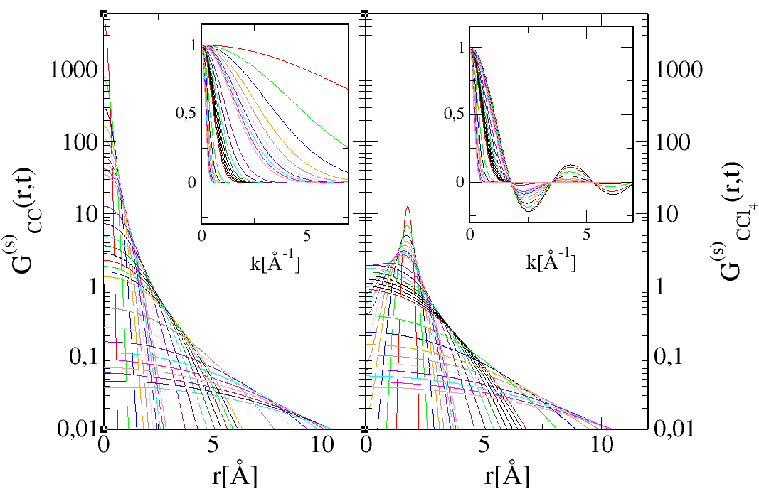
Figure 1: CCl₄: comparison of Self correlations $G^{(s)}(r,t)$ and $F^{(s)}(k,t)$ (inset) for carbon-carbon (left panel) and carbon-chloride (right panel) pairs of sites. The lines correspond to the 29 times selected (see text for curve plotting conventions). Note the vertical log-scale for the main panel.

The most notable features are the Dirac delta functions, one at $r=0$ for $G_{CC}^{(s)}(r,t=0)$ (left panel), whose Fourier transform (FT) is the black horizontal line in the inset, and the other at $r_{d}=2\mathring{A}$ for the C-Cl intermolecular distance (right panel), whose FT is $j_{0}(kr_{d})$ leads to the marked oscillations observed in the inset. Another interesting feature is that, although the $G^{(s)}(r,t)$ look Gaussian-like, they cannot be well fitted to Gaussians. This feature invalidates the usual Gaussian approximation $G^{(s)}(r,t)=\exp(-r^{2}/(4Dt)/(4\pi Dt)^{3/2}$ [47, 67, 68]. This is equally true of the small-$k$ Gaussian approximation of $F^{(s)}(k,t)\approx\exp(-Dk^{2}t)$.

Fig.2 shows the distinct part of the van Hove function $G^{(d)}(r,t)$ between the carbon atoms (left panel) and the carbon-tetrachloride in the right panel. Basically, these curves look like usual $g(r)$, but damped in time, as all the curves relax to 1 with time.

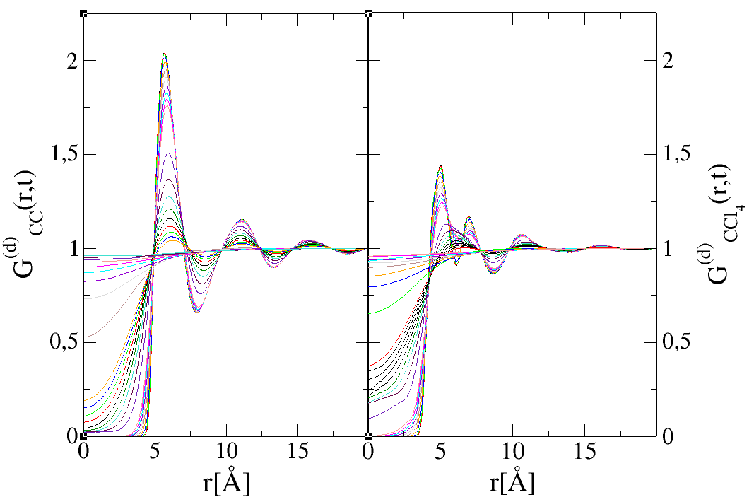
Figure 2: CCl₄: comparison of distinct van Hove functions $G^{(d)}(r,t)$ for carbon-carbon (left panel) and carbon-chloride (right panel) pairs of sites.

The most notable feature is the shift of the first peak of $G_{CCl_{4}}^{(d)}(r,t)$ to larger $r$-values after $t=1$ps, while the second peak is totally damped. It indicates a remarkable short time decorrelation of the central carbon with respect to the 4 LJ sites within this time range of $1$ps. It is equally worth noting that the replacement of the central particle at the core is not fully relaxed even after 100ps. It shows a slow diffusion of the molecule from its initial position.

Fig.3 shows the total intermediate scattering function $F^{(t)}(k,t)$ for the same 2 previous cases. These curves show remarkable features. First of all, we notice that at $t=0$, $F_{CC}^{(t)}(k,t=0)$ is exactly the static structure factor $S_{CC}(k)$, with the standard definition $S_{ab}(k)=\delta_{ab}+\rho\int d\mathbf{r}\exp(i\mathbf{k.r)}\left[g_{ab}(r)-1\right]$. However, in the present case, the asymptote term $\delta_{ab}$ is related to the intra-molecular correlation, and since $G^{s}(r,t=0)=\delta(r)/\rho$, it is this term which gives the $\delta_{ab}$ term, which is the asymptote 1 in case of the CC correlations.

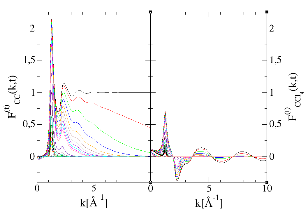
Figure 3: CCl₄: comparison of total intermediate scattering functions $F^{(s)}(k,t)$ for carbon-carbon (left panel) and carbon-chloride (right panel) pairs of sites.

The most important feature is that the plot shows clearly the decay of the asymptote with time. The large oscillations in the $F_{CCl_{4}}^{(t)}(k,t)$ are coming from the same self part $j_{0}(kr_{d})$ that is shown in the right inset of Fig.1.

Fig.4 show the total dynamical structure factor $S^{(t)}(k,\omega)$ and the self part in the inset, for the same atoms as above. The frequencies $\omega$ correspond to the times on the time grid described earlier, using the formula $\omega=2\pi/t$, and they are in units of ps^-1 which is also Ghz. The explicit values are There are 2 remarkable features. The first is that the main peak of $S(k,\omega)$ coincides with that of $F(k,t)$ in both cases. The second feature is that the self part looks very much like the usual Lorentzian approximation [47] $S^{(s)}(k,\omega)=Dk^{2}/\pi(\omega^{2}+(Dk^{2})^{2})$, but cannot be fully fitted to this simple form.

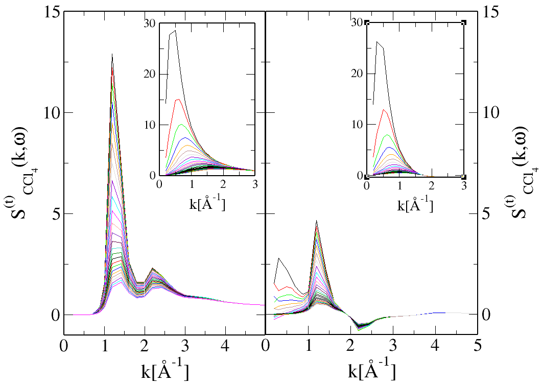
Figure 4: CCl₄: comparison of total dynamical structure factors $S^{(s)}(k,\omega)$ and corresponding self parts $S^{(s)}(k,\omega)$ (inset) for carbon-carbon (left panel) and carbon-chloride (right panel) pairs of sites. The lines correspond to the different $\omega=2\pi/t$ frequencies corresponding to the time grid in the $G(r,t)$ plots.

4.1.2 Polar liquid: acetone

Acetone is polar molecule, with dipole moment of $10\times 10^{20}$C$\mathring{A}$. Yet, there is no micro-structure formation in this liquid, other than the usual fluctuations, some related in part to dipole correlations. We can consider this liquid as a simple disorder liquid.

Fig.5 shows the oxygen-oxygen self van Hove function $G_{OO}^{(s)}(r,t)$ in the left panel and the corresponding self-intermediate scattering function $F_{OO}^{(s)}(k,t)$ in the inset, as well as the corresponding functions for the oxygen-carbon dynamical correlations in the right panel for $G_{OC}^{(s)}(r,t)$ and its inset for $F_{OC}^{(s)}(k,t)$. These curves have strong similarities with those for CCL4 in Fig.1.

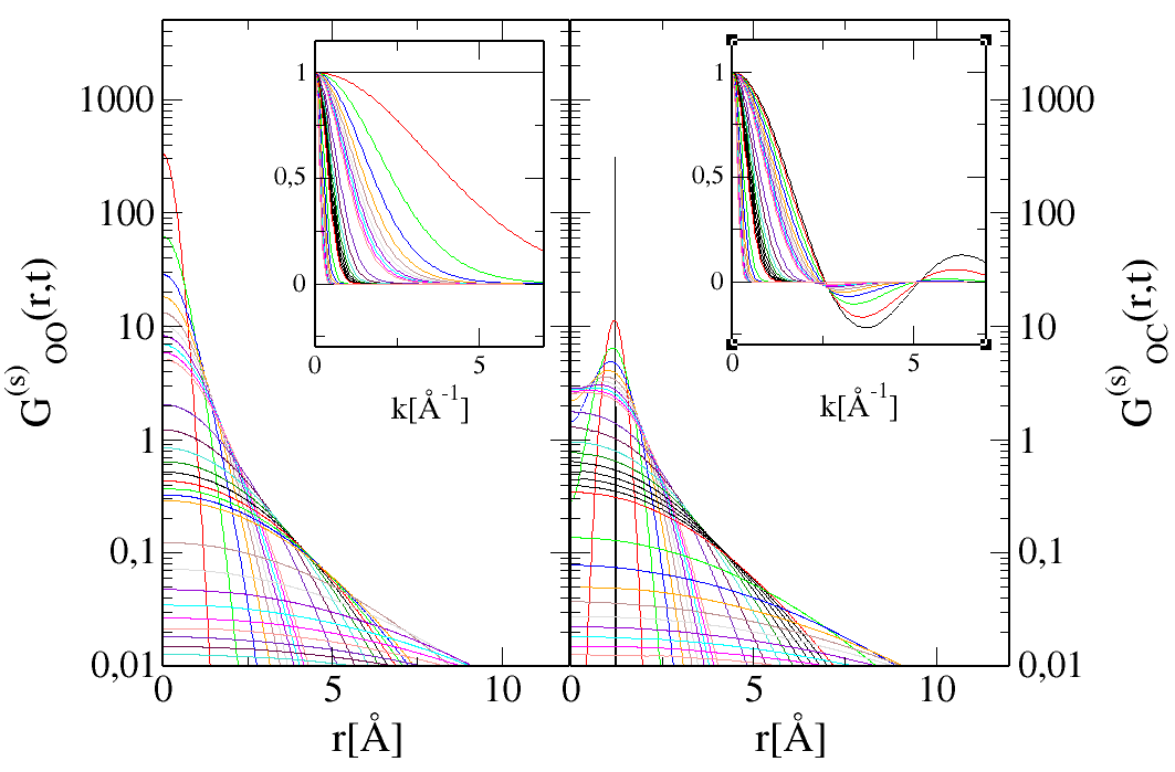
Figure 5: Acetone: comparison of Self correlations $G^{(s)}(r,t)$ and $F^{(s)}(k,t)$ (inset) for oxygen-oxygen (left panel) and oxygen-carbon (right panel) pairs of sites. The lines correspond to the 29 times selected (see text for curve plotting conventions). Note the vertical log-scale for the main panel.

They also show characteristic differences. The $r$-decay and the time decay in $r$-space are faster for acetone than for CCl₄. However, since all $G^{(s)}(r,t)$ integrate to 1 (that is $F^{(s)}(k=0,t)=1),$it means that self correlations are longer ranged for acetone than CCl₄, and especially at larger times. We can attribute this to dipole correlation with neighbours. However, it can be seen from the inset that $F_{OO}^{(s)}(k,t)$ decay faster for acetone than for CCl₄. We speculatively attribute this to CCl₄ being more “spherical” than acetone, possibly because of the dipole moment of the latter.

Fig.6 shows the time decay of distinct van Hove correlations for OO and OC. These are basically the equivalent of time dependent pair correlation functions since $g(r)=G^{(d)}(r,t=0)$, which is why they are worth analyzing. The comparison with CCl₄ in Fig.2 shows remarkable differences. For acetone, the main peaks are much smaller and the spatial oscillations much less pronounced (faster decay of spatial correlations). This is surprising since both liquids are dense. Again, this can be attributed to dipole correlations, using the following argument. The maintenance of dipole alignments can be achieved by several molecular positions, hence, for entropic reasons, there would be a faster decorrelation between sites, while the dipole correlations are maintained for longer times.

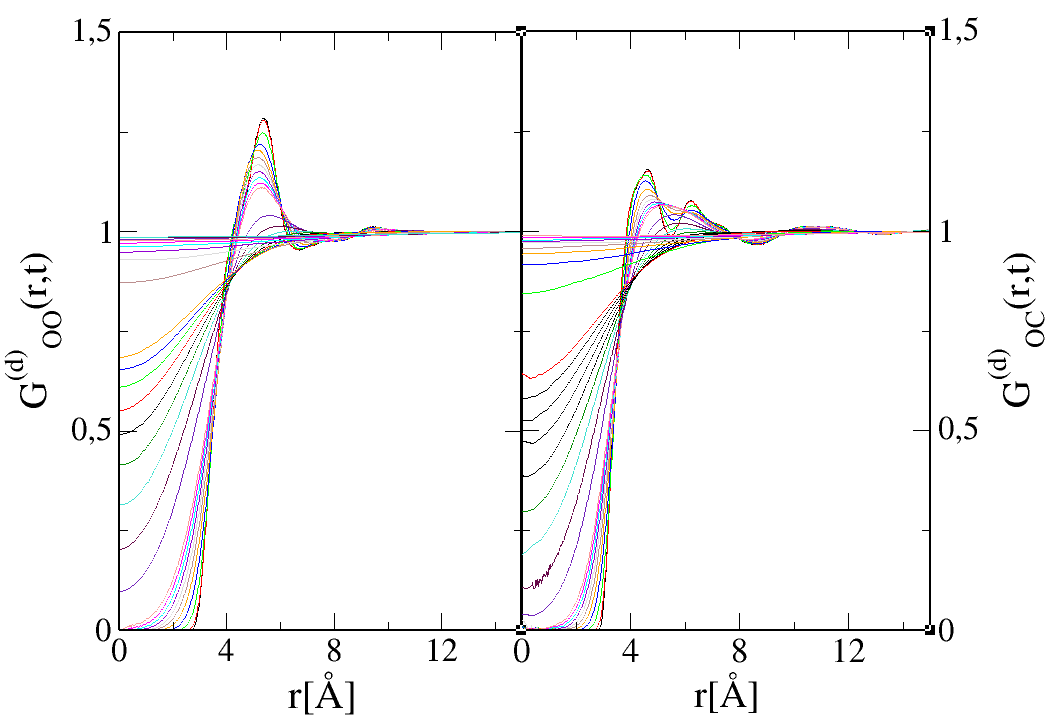
Figure 6: Acetone: comparison of distinct van Hove functions $G^{(d)}(r,t)$ for oxygen-oxygen (left panel) and oxygen-carbon (right panel) pairs of sites.

We note that the first peak spreading with time in the cross site correlation is very similar to that of CCl₄.

Fig.7 shows the total intermediate scattering function for the same two pairs of sites. We observe the same faster temporal decay for acetone thane for CCl₄, as that observed for the self part in the insets of Fig.5.

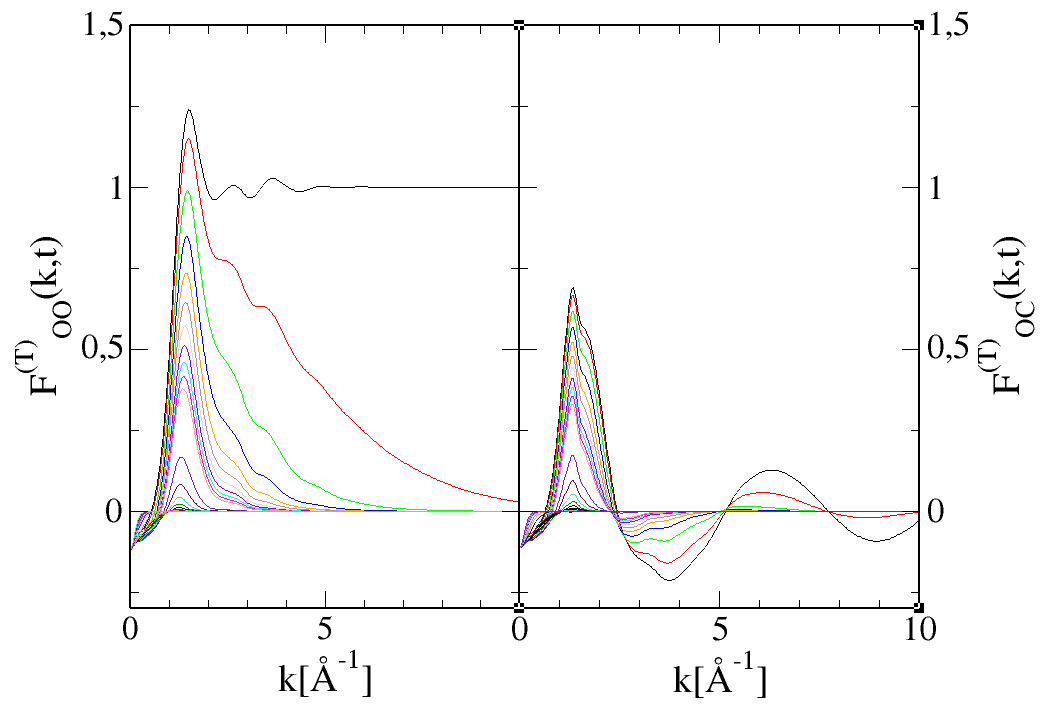
Figure 7: Acetone: comparison of total intermediate scattering functions $F^{(s)}(k,t)$ for oxygen-oxygen (left panel) and oxygen-carbon (right panel) pairs of sites.

The oscillations of the OC cross-correlations are also larger for acetone than for CCl₄. But this can be interpreted as a Fourier transform mathematical consequence of the core and first peak parts of the $G^{(d)}$function: the higher the first peak, the tighter the oscillations in $k$-space.

Fig.8 shows the total and self(inset) dynamical structure factors. The most prominent differences with CCl₄ of Fig.4 are the absence of second peak around $k\approx 2\mathring{A}$, and the small negative part near $k\approx 0$. The negative part is in fact a numerical artifact coming from the small negative part near $k=0$ of the $F(k,t)$ in Fig.7. This negative part is coming from a known problem in g(r), hence G(r,t), asymptote in simulations: they do not tend exactly to 1, but slightly below [69]. This problem is well known for the Kirkwood-Buff calculation in computer simulations [27, 30, 31, 32, 33].

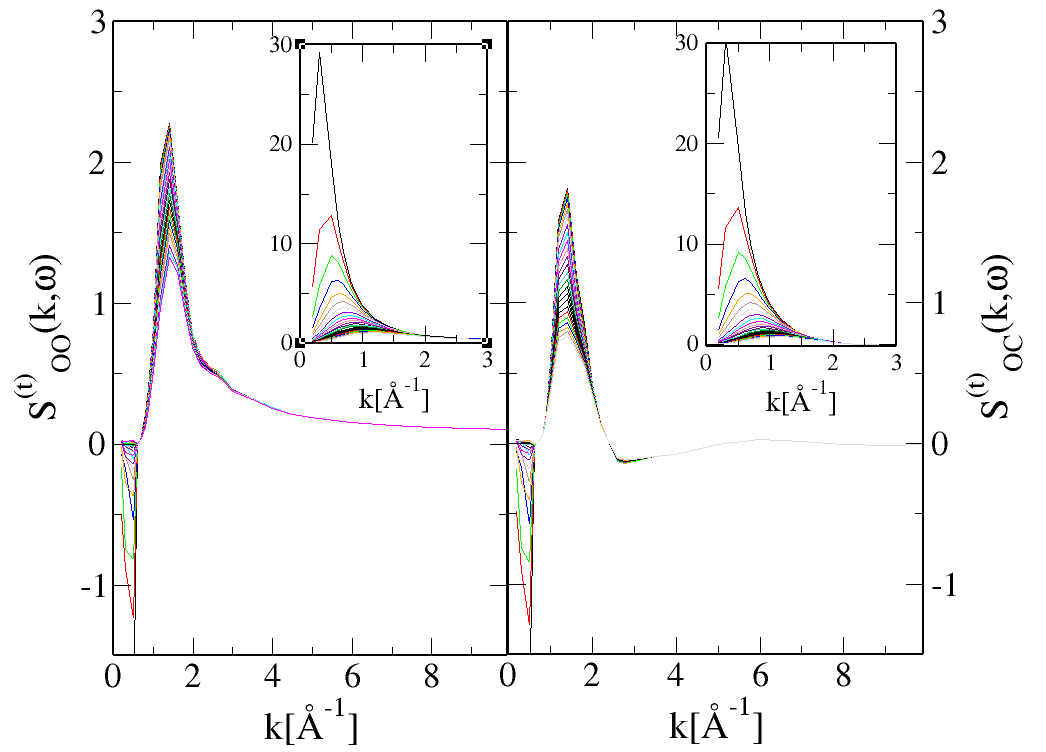
Figure 8: Acetone: comparison of the total dynamical structure factors $S^{(s)}(k,\omega)$ and corresponding self parts $S^{(s)}(k,\omega)$ (inset) for oxygen-oxygen (left panel) and oxygen-carbon (right panel) pairs of sites.

Aside from these, both sets of curves for CCl₄ and acetone look quite similar.

4.2 Complex disorder liquids

Herein, we study water and ethanol, which are both archetypical examples of hydrogen bonded liquids. We do not expect the self parts to show much differences, unless indirectly, since most of differences are related to the distinct part which contain the specific inter-molecular parts which make the difference between strongly and weakly clustered liquids.

4.2.1 Water

Fig.9 shows the self van Hove correlations both in $r$ and $k$(inset) space. The comparison with the simple disorder counter parts of CCl₄ and acetone in Figs[1,5], shows that there is quite a bit of resemblance with both of them. Perhaps the most importance difference is the smaller height of the main peaks, both at $r=0$ and $r=1\mathring{A}$ , and the faster decay in $r$-space. This is an important feature, since, because $F^{(s)}(k=0,t)=1$, it implies the existence of longer ranged $r$-correlations for water, which is an indirect proof of the Hbond network persistence for this particular liquid, over their absence for simple disorder liquids. Despite this difference, we observe that the $F^{(s)}(r,t)$ are quite similar.

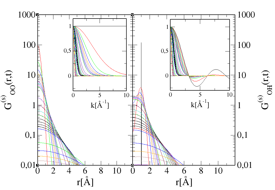
Figure 9: Water: comparison of Self correlations $G^{(s)}(r,t)$ and $F^{(s)}(k,t)$ (inset) for oxygen-oxygen (left panel) and oxygen-hydrogen (right panel) pairs of sites. The lines correspond to the 29 times selected (see text for curve plotting conventions). Note the vertical log-scale for the main panel.

This is, speculatively, an indication that water is a 2-state liquid: it appears as a r-space long range correlated liquid, and at the same time a disordered one in k-space. This is probably an typical difference, specially when comparing with the $F^{(s)}$ for acetone in Fig.5, which also appear as long ranged in r-space (as discussed previously sub-section 4.1.2), but differs in k-space.

Fig.10 shows the distinct dynamical correlations. Since $g_{OO}(r)=G_{OO}^{(d)}(r,t=0)$ we can observe the typical pair correlation of water, which differs considerably from that of simple disorder liquids, such as illustrated by CCl₄ and acetone, and its decay with time. The most striking difference is the rapid decay of the O-O contact peak at $r\approx 3\mathring{A}$ and the O-H Hbond peak at $r\approx 2\mathring{A}$ . This appears at first quite contradictory, since on would think that the Hbond related peaks should show more persistence than the contact peak of simple disorder liquids. This in fact similar to that observed for the self-functions above: what is important is not how rapidly the Hbond correlations are lost, but how rapidly they are reestablished. The latter is better observed in k-space (see below). Nevertheless, it appears that Hbonding has a very short life time since it decays very fast, which we have already observed in our previous work [70].

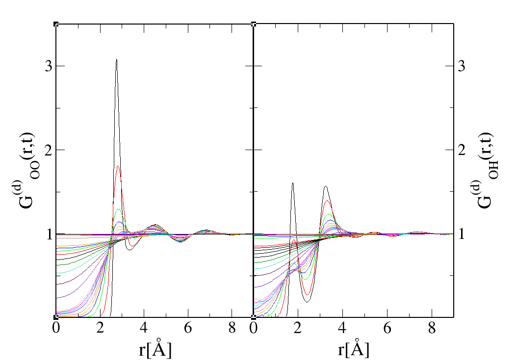
Figure 10: Comparison of distinct van Hove functions $G^{(d)}(r,t)$ for oxygen-oxygen (left panel) and oxygen-hydrogen (right panel) pairs of sites.

The above analysis is further confirmed in Fig.11, which shows the total intermediate scattering functions. We observe the typical split-peak feature of the structure factor of water, since $S_{OO}(k)=F_{OO}^{(t)}(k,t=0)$. But what seems interesting is that the shoulder peak at $k\approx 2\mathring{A}^{-1}$ ($r\approx 3\mathring{A}$) decays more slowly than the Hbond peak at $k\approx 3\mathring{A}^{-1}$($r\approx 2\mathring{A}$). We have recently proposed [71] that the shoulder peak is in fact the cluster peak for water, which points to water as forming mostly a dimer, which is a direct consequence of charge order. This is further confirmed by the fact that at $r\approx 3\mathring{A}$we observe an anti-peak in the OH correlations.

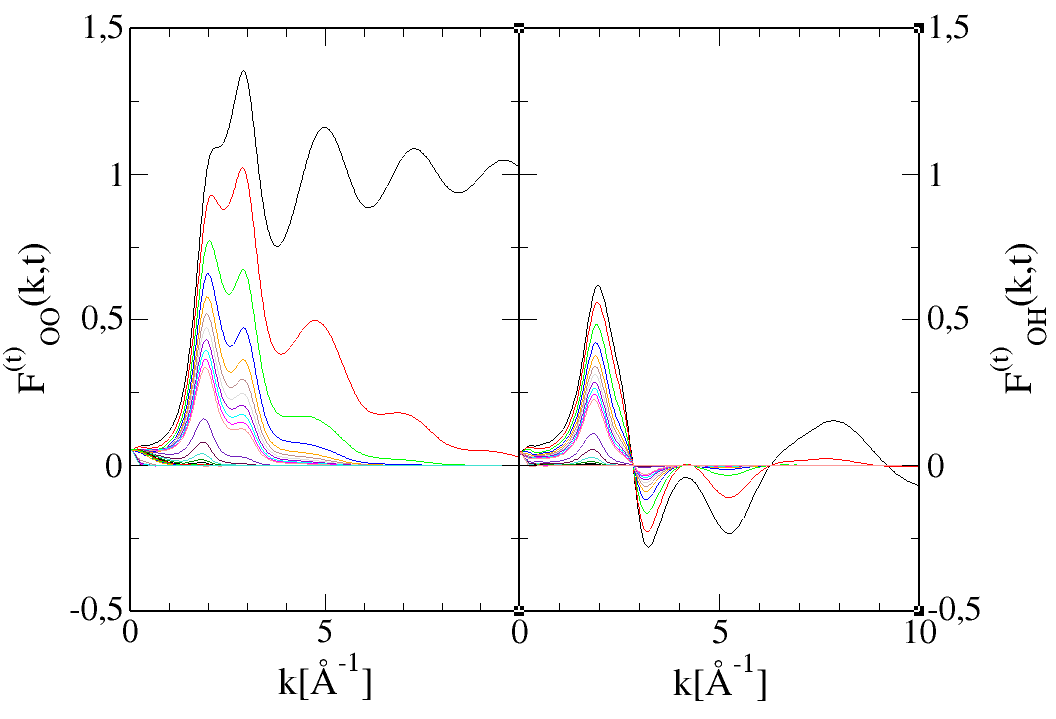
Figure 11: Water: comparison of total intermediate scattering functions $F^{(s)}(k,t)$ for oxygen-oxygen (left panel) and oxygen-hydrogen (right panel) pairs of sites.

Interestingly, the asymmetry of the time decay of these 2 peaks is very strongly reminiscent of their temperature dependence [72]: the Hbond peak is lost more quickly by heating than the contact-cluster peak.

Fig.12 shows the dynamical structure factors for the OO and OH atom pairs. The most striking feature is the small-k peak at $k\approx 0.3\mathring{A}^{-1}$, which corresponds to $r\approx 20\mathring{A}$. This peak is even more prominent for the OH correlations, indicating that its origin is mostly from the Hbond correlations. This peak is more important than dual peak that we observe at $k\approx 2\mathring{A}^{-1}$ and $k\approx 3\mathring{A}^{-1}$, which are directly related to those in Fig.11. In fact, this new peak is the dynamical equivalent of static pre-peak in the static structure factor.

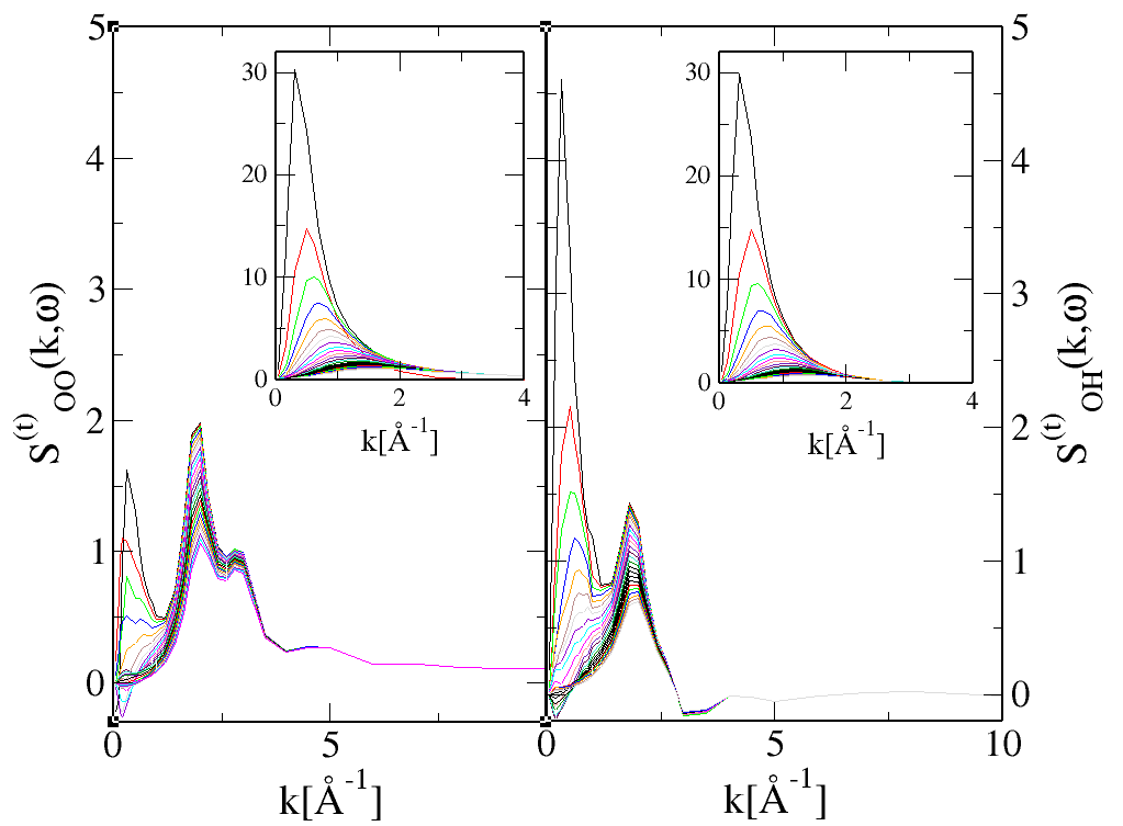
Figure 12: Water: comparison of the total dynamical structure factors $S^{(s)}(k,\omega)$ and corresponding self parts $S^{(s)}(k,\omega)$ (inset) for oxygen-oxygen (left panel) and oxygen-hydrogen (right panel) pairs of sites.

The distance size of $20\mathring{A}$ corresponds to a radius of $10\mathring{A}$, which is about the range of the marked oscillations in the $g_{OO}(r)$: the “3 peak structure” discussed in our previous work [73]. It this represent a kinetic clustering, as opposed to the static clustering which is observed through the pre-peak of the static structure factor. This analysis is further confirmed in the the case of ethanol below.

4.2.2 Ethanol

Contrary to water, alcohols have a well defined scattering pre-peak [16, 18, 19, 17, 20, 8, 74, 75, 9]. Herein, we focus on the case of ethanol for illustrative purposes.

Fig.13 shows the self parts of van Hove and intermediate scattering (insets) functions for OO and OH correlations. The general features are not so much different than that observed form the simple disorder liquids, which gives the false impression that the decorrelation of a single ethanol molecule is similar to that of CCl₄ or acetone.

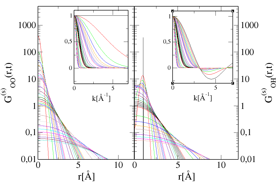
Figure 13: Ethanol: comparison of Self correlations $G^{(s)}(r,t)$ and $F^{(s)}(k,t)$ (inset) for oxygen-oxygen (left panel) and oxygen-hydrogen (right panel) pairs of sites. The lines correspond to the 29 times selected (see text for curve plotting conventions). Note the vertical log-scale for the main panel.

This is quite interesting, in the sense that water stands apart, even though both water and alcohols are Hbonded liquids, since we already observed distinct features at the level of the self dynamical correlations for this particular liquid.

In order to find the specificity related to Hbonding, we turn towards the distinct correlation functions in Fig.14. We observe several similarities with water. The high first peak is a witness of Hbonding, just like water, and it is also seen to decay very fast. A specificity of alcohols is the depletion correlations after the main peak, which are at the origin of the alcohol pre-peak [2, 25].

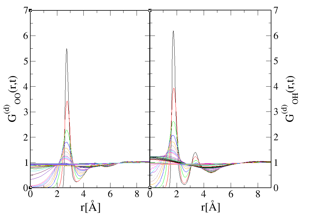
Figure 14: Ethanol: comparison of distinct van Hove functions $G^{(d)}(r,t)$ for oxygen-oxygen (left panel) and oxygen-hydrogen (right panel) pairs of sites.

These depletion correlation of the second and higher neighbours are related to the chain formation of the hydroxyl groups, and express the fact that the corresponding neighbours are in reduced number with respect to full space filling. It is seen that the depleted region re-emerge above 1 around $r\approx 7-8\mathring{A}.$ These depletion correlations are seen to decay more slowly, a feature more visible in the Fourier transform discussed below.

Fig.15 shows how the pre-peak at $k_{PP}\approx 0.75-0.8\mathring{A}^{-1}$ ($r\approx 7-8\mathring{A}$) and Hbond peak at $k_{MP}\approx 3\mathring{A}^{-1}$ ($r\approx 2\mathring{A}$) of ethanol decay in time. $k_{PP}$ corresponds to the depletion range observed in Fig.14, while the main peak is exactly that of water and corresponds to the O-H Hbonding distance. Just like water, the cluster pre-peak is seen to decay much more slowly than the main peak. The rate of decay is seen to be even slower than the dimer cluster peak of water.

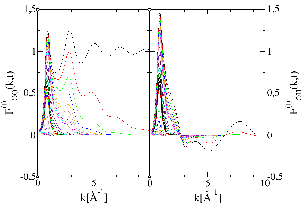
Figure 15: Ethanol: comparison of total intermediate scattering functions $F^{(s)}(k,t)$ for carbon-carbon (left panel) and carbon-chloride (right panel) pairs of sites.

This is in line with the fact that alcohol have long lived chain clusters [76, 70].

Fig.16 shows the dynamical structure factors for the OO and OH atom pairs. We observe a very high dynamical pre-peak at $k\approx 0.7-0.8\mathring{A}^{-1}$, similar to water, but much higher in magnitude, which corresponds exactly to the static pre-peak of ethanol observed above. In contrast to the case above, we see that the peak at $k\approx 3\mathring{A}$ is much smaller. These features highlight the dynamics of cluster formation in ethanol, and more generally in alcohols.

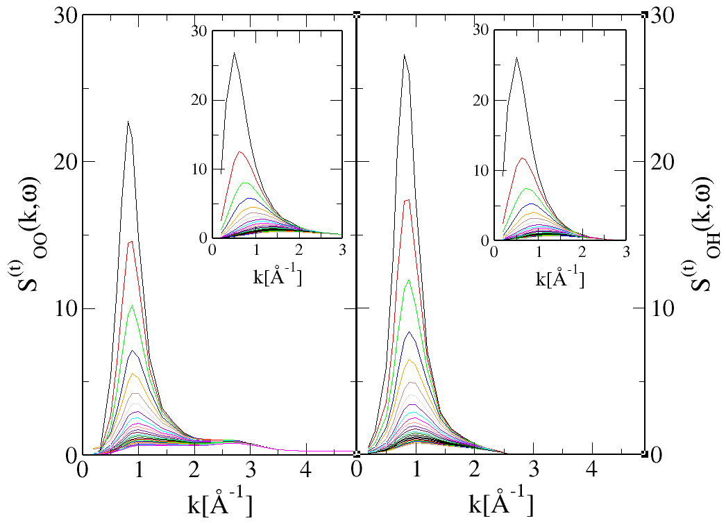
Figure 16: Ethanol: comparison of the total dynamical structure factors $S^{(s)}(k,\omega)$ and corresponding self parts $S^{(s)}(k,\omega)$ (inset) for oxygen-oxygen (left panel) and oxygen-hydrogen (right panel) pairs of sites.

This analysis reveals that the dynamical structure factors are better indicators of the cluster dynamics than the static structure factors, and highlight the underlying kinetics.

5 Conclusion

In this work, we have conducted an analysis of the dynamics of liquids are revealed by the pair correlation functions, both in $r$ and $k$ space, as well in time and frequency. To this end, the van Hove, intermediate scattering functions and dynamical structure factors have been calculated in computer simulations of model liquids. Having in mind the structural differences between simple disorder liquids and clustering liquids, we have studied CCl₄ and acetone for the first case, water and ethanol for the second case. Our study reveals that many important structural differences between the two categories of liquids exist, as exemplified by the analysis of the various dynamical pair correlation functions. The most important difference is the existence of kinetic processes due to clustering, which are prominently found in the small $k$ part of atom-atom dynamical structure factors $S(k,\omega)$ of complex disorder liquids, and are totally absent from the simple disorder liquids. This feature is not so much perceptible from the static structure factor $S(k)$ and intermediate scattering functions $F(k,t)$, as exemplified for the case of water. Since the x-ray radiation scattering experiments are related to the static structure factors, it appear important to refer to neutron scattering experiments in order to gain access to the dynamical scattering intensity. We expect that this work will motivate research in this direction.

References

- [1] Perera, A. From solutions to molecular emulsions. Pure and Applied Chemistry, 2016. 88, 189.
- [2] Požar, M.; Lovrinčević, B.; Zoranić, L.; Primorac, T.; Sokolić, F. and Perera, A. Micro-heterogeneity versus clustering in binary mixtures of ethanol with water or alkanes. Physical Chemistry Chemical Physics, 2016. 18, 23971.
- [3] Dixit, S.; Crain, J.; Poon, W.; Finney, J. and Soper, A. Molecular segregation observed in a concentrated alcohol-water solution. Nature, 2002. 416, 829.
- [4] Guo, J.H.; Luo, Y.; Augustsson, A.; Kashtanov, S.; Rubensson, J.E.; Shuh, D.K.; Ågren, H. and Nordgren, J. Molecular structure of alcohol-water mixtures. Phys. Rev. Lett., 2003. 91, 157401.
- [5] Warren, B. X-ray diffraction in long chain liquids. Phys. Rev., 1933. 44, 969.
- [6] Pierce, W. and MacMillan, D. X-ray studies on liquids: the inner peak for alcohols and acids. Journal of the American Chemical Society, 1938. 60, 779.
- [7] Benmore, C. and Loh, Y. The structure of liquid ethanol: A neutron diffraction and molecular dynamics study. The Journal of Chemical Physics, 2000. 112, 5877.
- [8] Tomšič, M.; Jamnik, A.; Fritz-Popovski, G.; Glatter, O. and Vlček, L. Structural properties of pure simple alcohols from ethanol, propanol, butanol, pentanol, to hexanol: Comparing monte carlo simulations with experimental saxs data. The Journal of Physical Chemistry B, 2007. 111, 1738.
- [9] Cerar, J.; Lajovic, A.; Jamnik, A. and Tomšič, M. Performance of various models in structural characterization of n-butanol: Molecular dynamics and x-ray scattering studies. Journal of Molecular Liquids, 2017. 229, 346 .
- [10] Perera, A.; Sokolić, F. and Zoranić, L. Microstructure of neat alcohols. Physical Review E, 2007. 75, 060502(R).
- [11] Prévost, S.; Gradzielski, M. and Zemb, T. Self-assembly, phase behaviour and structural behaviour as observed by scattering for classical and non-classical microemulsions. Advances in Colloid and Interface Science, 2017. 247, 374 .
- [12] Goddeeris, C.; Cuppo, F.; Reynaers, H.; Bouwman, W. and den Mooter, G.V. Light scattering measurements on microemulsions: Estimation of droplet sizes. International Journal of Pharmaceutics, 2006. 312, 187 .
- [13] Teubner, M. and Strey, R. Origin of the scattering peak in microemulsions. The Journal of Chemical Physics, 1987. 87(5), 3195.
- [14] Kundu, N.; Banik, D. and Sarkar, N. Self-assembly of amphiphiles into vesicles and fibrils: Investigation of structure and dynamics using spectroscopy and microscopy techniques. Langmuir, 2018. 34(39), 11637. PMID: 29544249.
- [15] Magini, M.; Paschina, G. and Piccaluga, G. On the structure of methyl alcohol at room temperature. The Journal of Chemical Physics, 1982. 77, 2051.
- [16] Narten, A. and Habenschuss, A. Hydrogen bonding in liquid methanol and ethanol determined by x-ray diffraction. The Journal of Chemical Physics, 1984. 80, 3387.
- [17] Vahvaselkä, K.S.; Serimaa, R. and Torkkeli, M. Determination of liquid structures of the primary alcohols methanol, ethanol, 1-propanol, 1-butanol and 1-octanol by x-ray scattering. Journal of Applied Crystallography, 1995. 28, 189.
- [18] Sarkar, S. and Joarder, R.N. Molecular clusters and correlations in liquid methanol at room temperature. The Journal of Chemical Physics, 1993. 99, 2032.
- [19] Sarkar, S. and Joarder, R.N. Molecular clusters in liquid ethanol at room temperature. The Journal of Chemical Physics, 1994. 100, 5118.
- [20] Karmakar, A.; Krishna, P. and Joarder, R. On the structure function of liquid alcohols at small wave numbers and signature of hydrogen-bonded clusters in the liquid state. Physics Letters A, 1999. 253, 207.
- [21] Nishikawa, K. and Iijima, T. Small-angle x-ray scattering study of fluctuations in ethanol and water mixtures. The Journal of Physical Chemistry, 1993. 97, 10824.
- [22] Akiyama, I.; Ogawa, M.; Takase, K.; Takamuku, T.; Yamaguchi, T. and Ohtori, N. Liquid structure of 1-propanol by molecular dynamics simulations and x-ray scattering. Journal of Solution Chemistry, 2004. 33, 797.
- [23] Takamuku, T.; Maruyama, H.; Watanabe, K. and Yamaguchi, T. Structure of 1-propanol-water mixtures investigated by large-angle x-ray scattering technique. Journal of Solution Chemistry, 2004. 33, 641.
- [24] Almásy, L.; Kuklin, A.; Požar, M.; Baptista, A. and Perera, A. Microscopic origin of the scattering pre-peak in aqueous propylamine mixtures: X-ray and neutron experiments versus simulations. Phys. Chem. Chem. Phys., 2019. 21, 9317.
- [25] Požar, M.; Bolle, J.; Sternemann, C. and Perera, A. On the x-ray scattering pre-peak of linear mono-ols and the related microstructure from computer simulations. J. Phys. Chem. B, 2020. 124(38), 8358.
- [26] Anisimov, D.S.D.A.I.I.K.Y.M.A. and Sengers, J.V. Mesoscale inhomogeneities in aqueous solutions of 3-methylpyridine and tertiary butyl alcohol. Journal of Chemical and Engineering Data, 2011. 56(4), 1238.
- [27] Perera, A. and Sokolić, F. Modeling nonionic aqueous solutions: The acetone-water mixture. The Journal of Chemical Physics, 2004. 121, 11272.
- [28] Ploetz, E. and Smith, P. A kirkwood-buff force field for the aromatic amino acids. Physical Chemistry Chemical Physics, 2011. 13, 18154.
- [29] Gupta, R. and Patey, G.N. Aggregation in dilute aqueous tert-butyl alcohol solutions: Insights from large-scale simulations. The Journal of Chemical Physics, 2012. 137(3), 034509.
- [30] Ganguly, P. and van der Vegt, N. Convergence of sampling kirkwood-buff integrals of aqueous solutions with molecular dynamics simulations. Journal of Chemical Theory and Computation, 2013. 9(3), 1347. PMID: 26587597.
- [31] Krüger, P.; Schnell, S.; Bedeaux, D.; Kjelstrup, S.; Vlugt, T. and Simon, J.M. Kirkwood-buff integrals for finite volumes. The Journal of Physical Chemistry Letters, 2013. 4(2), 235. PMID: 26283427.
- [32] Milzetti, J.; Nayar, D. and van der Vegt, N. Convergence of kirkwood-buff integrals of ideal and nonideal aqueous solutions using molecular dynamics simulations. The Journal of Physical Chemistry B, 2018. 122(21), 5515. PMID: 29342355.
- [33] Dawass, N.; Krüger, P.; Schnell, S.; Bedeaux, D.; Kjelstrup, S.; Simon, J. and Vlugt, T. Finite-size effects of kirkwood-buff integrals from molecular simulations. Molecular Simulation, 2018. 44, 599.
- [34] Rahman, A. Density fluctuations in liquid rubidium. ii. molecular-dynamics calculations. Phys. Rev. A, 1974. 9, 1667.
- [35] Yoshida, F. Dynamical structure factor in liquid rubidium. Journal of Physics F: Metal Physics, 1978. 8(3), 411.
- [36] Sjogren, L. Short-wavelength density fluctuations in liquid metals. Journal of Physics C: Solid State Physics, 1979. 12(3), 425.
- [37] Ebbsio, I.; Kinell, T. and Waller, I. The dynamical structure factor for liquid aluminium. Journal of Physics C: Solid State Physics, 1980. 13(10), 1865.
- [38] Kahol, P.K.; Chaturvedi, D.K. and Pathak, K.N. Dynamical structure factors in binary liquids. i. molten rbbr. Journal of Physics C: Solid State Physics, 1977. 10(21), 4181.
- [39] Moe, N.E. and Ediger, M.D. Calculation of the coherent dynamic structure factor of polyisoprene from molecular dynamics simulations. Phys. Rev. E, 1999. 59, 623.
- [40] Handle, P.H.; Rovigatti, L. and Sciortino, F. -independent slow dynamics in atomic and molecular systems. Phys. Rev. Lett., 2019. 122, 175501.
- [41] Wu, B.; Iwashita, T. and Egami, T. Atomic dynamics in simple liquid: de gennes narrowing revisited. Phys. Rev. Lett., 2018. 120, 135502.
- [42] Noguere, G.; Scotta, J.P.; Xu, S.; Farhi, E.; Ollivier, J.; Calzavarra, Y.; Rols, S.; Koza, M. and Marquez Damian, J.I. Temperature-dependent dynamic structure factors for liquid water inferred from inelastic neutron scattering measurements. The Journal of Chemical Physics, 2021. 155(2). 024502.
- [43] Alvarez, F.; Arbe, A. and Colmenero, J. Unraveling the coherent dynamic structure factor of liquid water at the mesoscale by molecular dynamics simulations. The Journal of Chemical Physics, 2021. 155(24). 244509.
- [44] Kežić, B. and Perera, A. Towards a more accurate reference interaction site model integral equation theory for molecular liquids. The Journal of Chemical Physics, 2011. 135(23). 234104.
- [45] Gray, C.G. and Gubbins, K.E. Theory of molecular fluids. Oxford University Press, New York, 1984.
- [46] Blum, L. and Torruella, A., J. Invariant expansion for two-body correlations: Thermodynamic functions, scattering, and the ornstein–zernike equation. J. Chem. Phys., 2003. 56(1), 303.
- [47] Hansen, J.P. and McDonald, I. Theory of Simple Liquids. Academic Press, Elsevier, Amsterdam, 3rd edition, 2006.
- [48] Hirata, F. Theory of Molecular Liquids, pages 1–60. Springer Netherlands, Dordrecht, 2003.
- [49] Debye, P. Zerstreuung von rontgenstrahlen. Annalen der Physik, 1915. 351, 809.
- [50] Debye, P. Scattering of x-rays. In The collected papers of Peter J.W. Debye. Interscience Publishers, 1954.
- [51] Pronk, S.; Páll, S.; Schulz, R.; Larsson, P.; Bjelkmar, P.; Apostolov, R.; Shirts, M.; Smith, J.; Kasson, P.; van der Spoel, D.; Hess, B. and Lindahl, E. Gromacs 4.5: a high-throughput and highly parallel open source molecular simulation toolkit. Bioinformatics, 2013. 29, 845.
- [52] Martínez, J. and Martínez, L. Packing optimization for automated generation of complex system’s initial configurations for molecular dynamics and docking. Journal of Computational Chemistry, 2003. 24, 819.
- [53] Nose, S. A molecular dynamics method for simulations in the canonical ensemble. Molecular Physics, 1984. 52, 255.
- [54] Hoover, W. Canonical dynamics: Equilibrium phase-space distributions. Physical Review A, 1985. 31, 1695.
- [55] Parrinello, M. and Rahman, A. Crystal structure and pair potentials: A molecular-dynamics study. Physical Review Letters, 1980. 45, 1196.
- [56] Parrinello, M. and Rahman, A. Polymorphic transitions in single crystals: A new molecular dynamics method. Journal of Applied Physics, 1981. 52, 7182.
- [57] Darden, T.; York, D. and Pedersen, L. Particle mesh ewald: An n*log(n) method for ewald sums in large systems. The Journal of Chemical Physics, 1993. 98, 10089.
- [58] Hess, B.; Bekker, H.; Berendsen, H. and Fraaije, J. Lincs: A linear constraint solver for molecular simulations. Journal of Computational Chemistry, 1997. 18, 1463.
- [59] Berendsen, H.J.C.; Grigera, J.R. and Straatsma, T.P. The missing term in effective pair potentials. The Journal of Physical Chemistry, 1987. 91(24), 6269.
- [60] Jorgensen, W. Optimized intermolecular potential functions for liquid alcohols. The Journal of Physical Chemistry, 1986. 90(7), 1276.
- [61] Duffy, E.; Severance, D. and Jorgensen, W. Solvent effects on the barrier to isomerization for a tertiary amide from ab initio and monte carlo calculations. Journal of the American Chemical Society, 1992. 114(19), 7535.
- [62] Jorgensen, W.; Briggs, J. and Contreras, M. Relative partition coefficients for organic solutes from fluid simulations. The Journal of Physical Chemistry, 1990. 94(4), 1683.
- [63] Požar, M. and Zoranić, L. The structuring in mixtures with acetone as the common solvent. Physics and Chemistry of Liquids, 2020. 58(2), 184.
- [64] Požar, M.; Jukić, I. and B., L. Thermodynamic, structural and dynamic properties of selected non-associative neat liquids. Journal of Physics: Condensed Matter, 2020. 32(405101).
- [65] Walter, N.; Jaiswal, A.; Cai, Z. and Zhang, Y. Liquidlib: A comprehensive toolbox for analyzing classical and ab initio molecular dynamics simulations of liquids and liquid-like matter with applications to neutron scattering experiments. Computer Physics Communications, 2018. 228, 209 .
- [66] Perera, A. and Mazighi, R. Simple and complex forms of disorder in ionic liquids. Journal of Molecular Liquids, 2015. 210, 243. Mesoscopic structure and dynamics in ionic liquids.
- [67] Boon, J.P. and Yip, S. Molecular Hydrodynamics. Dover Publications, Inc., New York, 1980.
- [68] Berne, B.J. and Pecora, R. Dynamic Light Scattering: With Applications to Chemistry, Biology, and Physics. John Wiley and Sons, Inc., 2000.
- [69] Lebowitz, J. and Percus, J. Long-range correlations in a closed system with applications to nonuniform fluids. Physical Review, 1961. 122(6), 1675.
- [70] Jukić, I.; Požar, M.; Lovrinčević, B. and Perera, A. Universal features in the lifetime distribution of clusters in hydrogen-bonding liquids. Phys. Chem. Chem. Phys., 2021. 23, 19537.
- [71] Lovrinčević, B.; Požar, M.; Jukić, I. and Perera, A. On the role charge ordering in the dynamics of cluster formation in associated liquids. ChemRxiv. Cambridge: Cambridge Open Engage, 2022. This content is a preprint and has not been peer-reviewed.
- [72] Amann-Winkel, K.; Bellissent-Funel, M.C.; Bove, L.E.; Loerting, T.; Nilsson, A.; Paciaroni, A.; Schlesinger, D. and Skinner, L. X-ray and neutron scattering of water. Chemical Reviews, 2016. 116(13), 7570.
- [73] Perera, A. On the microscopic structure of liquid water. Molecular Physics, 2011. 109(20), 2433.
- [74] Vrhovšek, A.; Gereben, O.; Jamnik, A. and Pusztai, L. Hydrogen bonding and molecular aggregates in liquid methanol, ethanol, and 1-propanol. The Journal of Physical Chemistry B, 2011. 115, 13473.
- [75] Sillrén, P.; Swenson, J.; Mattsson, J.; Bowron, D. and Matic, A. The temperature dependent structure of liquid 1-propanol as studied by neutron diffraction and epsr simulations. The Journal of Chemical Physics, 2013. 138, 214501.
- [76] Fujii, A.; Sugawara, N.; Hsu, P.J.; Shimamori, T.; Li, Y.C.; Hamashima, T. and Kuo, J.L. Hydrogen bond network structures of protonated short-chain alcohol clusters. Phys. Chem. Chem. Phys., 2018. 20, 14971.