Domain Generalization for Domain-Linked Classes

Abstract

Domain generalization (DG) focuses on transferring domain-invariant knowledge from multiple source domains (available at train time) to an a priori unseen target domain(s). This requires a class to be expressed in multiple domains for the learning algorithm to break the spurious correlations between domain and class. However, in the real-world, classes may often be domain-linked, i.e. expressed only in a specific domain, which leads to extremely poor generalization performance for these classes. In this work, we aim to learn generalizable representations for these domain-linked classes by transferring domain-invariant knowledge from classes expressed in multiple source domains (domain-shared classes). To this end, we introduce this task to the community and propose a Fair and cONtrastive feature-space regularization algorithm for Domain-linked DG FOND. Rigorous and reproducible experiments with baselines across popular DG tasks demonstrate our method and its variants’ ability to accomplish state-of-the-art DG results for domain-linked classes. We also provide practical insights on data conditions that increase domain-linked class generalizability to tackle real-world data scarcity.

Keywords Domain Generalization  $\cdot$ Fairness  $\cdot$ Transfer Learning

1 Introduction

Common data collection strategies for machine learning (ML) aggregate multiple data sources with the goal of generalizing the extracted knowledge to target application(s) (Nguyen et al., 2021b). ML models excel when both the source and target data are independent and identically distributed (i.i.d.) (Vapnik, 2000); this assumption is often violated in the real-world. This motivates the domain generalization (DG) task where learning algorithms seek to generalize to data distributions (domains) different from what was observed during training, i.e. out-of-distribution data.

Modern DG algorithms operate on the principle that learned representations that are invariant to different domains are more general and transferable to out-of-distribution data (Ye et al., 2021). As a result, recent works aim to explicitly reduce the representation discrepancy between multiple source-domains (Wang et al., 2021a), by leveraging distribution-alignment (Nguyen et al., 2021a; Sun and Saenko, 2016), domain-discriminative adversarial networks (Zhang et al., 2021; Albuquerque et al., 2019), domain-based feature-alignment (Ruan et al., 2022; Kim et al., 2021), and meta-learning approaches (Shu et al., 2021; Zhang et al., 2020; Li et al., 2017b). Most methods explicitly assume all classes are observed in multiple source-domains for the goal of disentangling spurious correlations between domain and class. Methods that omit this assumption still focus on overall accuracy, conversely ignoring the performance discrepancy between domain-linked and domain-shared classes.

In the real-world, there are often classes that are only observed in specific domains, (i.e., domain-linked classes $\mathcal{Y}_{L}$) (see Fig. 1(a)). For instance, in healthcare (Chen et al., 2021), autonomous vehicle (Piva et al., 2023), and fraud detection (Ataabadi et al., 2022) ML research, factors such as demographic imbalance, city infrastructure and privacy policy restrict the availability of classes expressed in multiple domains (i.e., domain-shared classes $\mathcal{Y}_{S}$). Existing DG approaches yield large performance discrepancies between $\mathcal{Y}_{L}$ and $\mathcal{Y}_{S}$ classes; see Fig. 1(b). In this paper, we seek to improve the performance for domain-linked $\mathcal{Y}_{L}$ classes. We ask the following question: Can we transfer domain-invariant representations learned from domain-shared classes to domain-linked classes?

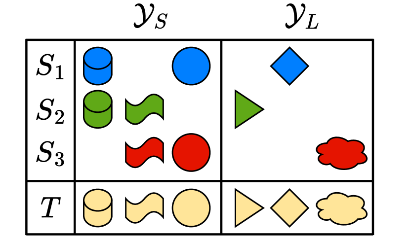
(a)

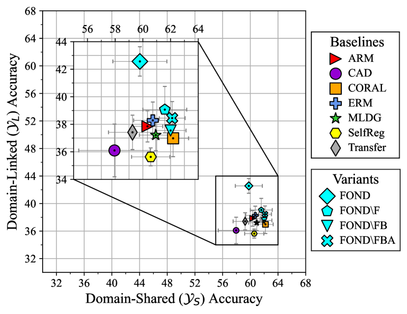
(b)

Figure 1: Illustration of domain-linked ($\mathcal{Y}_{L}$) and domain-shared ($\mathcal{Y}_{S}$) classes and resulting performance discrepancies. Panel (a) illustrates a shape classification task with domain-linked and domain-shared classes; the domains are represented by color. During training some classes are expressed in multiple domains (e.g. circle) while others are expressed in only one domain (e.g. triangle). Panel (b) communicates the performance discrepancy between $\mathcal{Y}_{L}$ and $\mathcal{Y}_{S}$ across all datasets (PACS, OfficeHome and VLCS) and different class-distribution settings (High, Low).

We answer this in the affirmative. Specifically, we draw insights from the field of fairness (Wang et al., 2020; Makhlouf et al., 2021) to transfer these generalizable representations from $\mathcal{Y}_{S}$ to $\mathcal{Y}_{L}$ classes. Note that recently Pham et al. (2023) studied fairness with the end goal of similar outcomes for protected attributes (such as gender). On the other hand, our work leverages fairness as a way to learn generalizable representations for domain-linked classes. We accomplish this by learning fair representations, which we define as representations that yield similar outcomes for domain-linked and domain-shared classes. We then develop a contrastive learning objective that carefully considers the pairwise relationships between same-class-inter-domain and different-class-intra-domain training samples to learn domain-invariant representations. Therefore, we propose the flexible contrastive and fair feature-space regularization algorithm FOND, (Fair and cONtrastive Domain-linked learning).

We rigorously evaluate FOND and DG baselines on three standard DG benchmark datasets, where FOND and its variants achieve performance improvements on PACS (Li et al., 2017a) (+2.9%), VLCS (Fang et al., 2013) (+20.3%), and OfficeHome (Venkateswara et al., 2017) (+1.1%). To this end, we analyze domain-linked generalization performance for different (a) target class sizes, (b) domain-variance types, and (c) domain-shared and domain-linked class distributions. Our key observation: FOND consistently outperforms baselines given a sufficient number for domain-shared classes to learn from. To the best of our knowledge this the first work to introduce and propose a method for domain-linked class representation learning, which can directly impact the real world applications of DG.

2 Related works

In this section, we briefly introduce domain generalization works related to this paper and identify the research gap this paper seeks to study. To reiterate, DG aims to learn a machine learning model that predicts well on distributions different from those seen during training. To achieve this, DG methods typically aim to minimize the discrepancy between multiple source-domains (Ye et al., 2021).

Data manipulation techniques primarily focus on data augmentation and generation techniques. Typical augmentations include affine transformations in conjunction with additive noise, cropping and so on (Shorten and Khoshgoftaar, 2019; He et al., 2015). Other methods include simulations (Tobin et al., 2017; Yue et al., 2019; Tremblay et al., 2018), gradient-based perturbations like CrossGrad (Shankar et al., 2018), adversarial augmentation (Volpi et al., 2018) and image mixing (e.g. CutMix (Mancini et al., 2020), Mixup (Zhang et al., 2018) and Dir-mixup (Shu et al., 2021)). Furthermore, generative models using VAEs GANs are also popular techniques for diverse data generation (Anoosheh et al., 2017; Zhou et al., 2020; Somavarapu et al., 2020; Huang and Belongie, 2017). Since the model generalizability is a consequence of training data diversity (Vapnik, 2000), FOND and other approaches should be used in conjunction. It is important to consider the complexity of data generation techniques since they often require observing classes in multiple domains.

Multi-domain feature alignment techniques primarily align features across source-domains through explicit feature distribution alignment. For example, DIRT (Nguyen et al., 2021a) align transformed domains, CORAL (Sun and Saenko, 2016) and M³SDA (Peng et al., 2019) align second and first-order statistics, MDA (Hu et al., 2019) learn class-wise kernels, and others use measures like Wasserstein distance (Zhou et al., 2021; Wang et al., 2021b). Other approaches learn invariant representations through domain-discriminative adversarial training (Zhu et al., 2022; Yang et al., 2021; Shao et al., 2019; Li et al., 2018; Gong et al., 2018). Most of these approaches explicitly, if not implicitly, assume all classes are domain-shared. Since there is a 1:1 correlation between $\mathcal{Y}_{L}$ classes and their domains, adversarial domain-discriminators may infer an inputs domain from class-discriminative features, i.e., the very same representations needed for the down-stream task.

Meta-learning approaches promote the generalizability of a model by imitating the generalization tasks through meta-train and meta-test objectives; MLDG (Li et al., 2017b) and ARM (Zhang et al., 2020) are popular base architectures (Zhong et al., 2022; Shu et al., 2021); interesting methods like Transfer (Zhang et al., 2021) combine meta-learning with adversarial training.

Contrastive learning aims is to learn representations , self-supervised (Chen et al., 2020) or supervised (Khosla et al., 2020; Motiian et al., 2017), such that similar samples are embedded close to each other while distancing dissimilar samples (Huang et al., 2020; Ruan et al., 2022; Kim et al., 2021; Khosla et al., 2020; Chen et al., 2020; Motiian et al., 2017). These methods make broad domain-aware comparisons which are insufficient for domain-linked class generalization.

Fairness notions in DG (Makhlouf et al., 2021) involve reducing the performance discrepancy between protected attributes (e.g. demographic) (Pham et al., 2023; Wang et al., 2020). However, our work enforces fairness to learn generalizable representations for domain-linked classes.

Research gap. Existing DG approaches presuppose all source-domain classes are expressed in multiple domains. Approaches that omit this assumption still seek to maximize average generalization; thus ignore the performance discrepancy between domain-linked and domain-shared classes. In this paper we explicitly seek to improve the generalizability of domain-linked $\mathcal{Y}_{L}$ classes.

3 Problem formulation

In this section we formally define a domain (Def. 3.1) is, the domain generalization (Def. 3.2) task, domain-linked/shared classes and the learning objective.

Definition 3.1 (Domain).

Let $\mathcal{X}$ denote an nonempty input space (e.g. images, text, etc) and $\mathcal{Y}$ an output label space. A domain $S$ is composed of data samples from a joint distribution $\mathcal{D}:\mathcal{X}\times\mathcal{Y}$. We denote as specific domain as $S_{i}=\{(\mathbf{x}_{i},y_{i})\}_{i=1}^{n}\sim\mathcal{D}_{i}:\mathcal{X}_{i}\times\mathcal{Y}_{i}$, where $\mathbf{x}\in\mathcal{X}\subseteq\mathbb{R}^{d}$ and $y\in\mathcal{Y}\subset\mathbb{R}$. Additionally, $X$ and $Y$ denote the corresponding random variables.

Given this definition of a domain, the DG task – which entails learning representations from multiple source-domains to generalize to unseen target-domain(s) – can be formalized in Def. 3.2.

Definition 3.2 (Domain generalization).

Given $K$ training (source) domains $\mathcal{S}=\{S^{i}~{}|~{}i=1,...,K\}$ where $\mathcal{S}_{i}=\{(\mathbf{x}^{i}_{j},y^{i}_{j})\}_{j=1}^{n_{i}}$ for the $i$-th domain and $n_{i}$ number of samples. The joint distributions between each pair of domains are different: $\mathcal{D}_{i}\neq\mathcal{D}_{j}:1\leq i\neq j\leq K$. Then the goal is to learn a predictive function from $\mathcal{S}$ to a achieve a reliable performance on an unseen, out-of-distribution, (test) target-domain $T\sim\mathcal{D}_{T}:\mathcal{X}_{T}\times\mathcal{Y}_{T}$ (i.e. $\mathcal{D}_{T}\neq\mathcal{D}_{i}$ for $i\in\{1,...,K\}$).

We evaluated methods for closed-set domain generalization (i.e. $\mathcal{Y}_{T}=\bigcup^{K}_{i=1}\mathcal{Y}_{i}$) where no source-domain expresses the full set of target classes (i.e., $\mathcal{Y}_{T}\subset\mathcal{Y}_{i}$ for $i\in\{1,...,K\}$). Furthermore, during training there exists classes expressed in only one source-domain (i.e. domain-linked $\mathcal{Y}_{L}$ classes) and those in multiple (i.e. domain-shared $\mathcal{Y}_{S}$ classes) where $\mathcal{Y}_{T}=\mathcal{Y}_{L}\cup\mathcal{Y}_{S}$ and $\mathcal{Y}_{L}\cap\mathcal{Y}_{S}=\emptyset$.

Learning objective. The learning objective is to identify a generalizable predictive function $M:\mathcal{X}\rightarrow\mathcal{Y}$ to achieve a minimum predictive error on an unseen, out-of-distribution, test domain $T$ under the previously outlined conditions. The task network is defined as $M=(F\circ G)(\mathbf{x})$, where $F:\mathcal{X}\rightarrow\mathcal{H}$ is the feature extractor and $G:\mathcal{H}\rightarrow\mathcal{Y}^{\Delta}$ is the classifier.

4 Methodology

Algorithm 1 Fair…(FOND) Training Algorithm

1:Source datasets $\mathcal{S}$, feature extractor $F$, projection network $P$, classification network $G$

2:while Not Converged do

3:     Sample a batch of data $\mathcal{B}=\{(\mathbf{x}_{1},\mathbf{y}_{1}),(\mathbf{x}_{1},\mathbf{y}_{1}),...,(\mathbf{x}_{K},\mathbf{y}_{K})\}$ from all source domains $\mathcal{S}$

4:     $\mathcal{B}_{F}=\{(\mathbf{h}_{1},\mathbf{y}_{1}),(\mathbf{h}_{2},\mathbf{y}_{2}),...,(\mathbf{h}_{K},\mathbf{y}_{K})\}\leftarrow F(\mathcal{B})$ $\triangleright$ Generate input representations

5:     $\mathcal{B}_{P}=\{(\mathbf{z}_{1},\mathbf{y}_{1}),(\mathbf{z}_{2},\mathbf{y}_{2}),...,(\mathbf{z}_{K},\mathbf{y}_{K})\}\leftarrow P(\mathcal{B}_{F})$ $\triangleright$ Generate feature projections

6:     $\mathcal{L}_{xdom}\leftarrow\{\mathcal{B}_{P},\alpha,\beta\}$ $\triangleright$ Calculate domain-aware loss according to Eq. (2)

7:     $\mathcal{B}_{C}\leftarrow G(\mathcal{B}_{F})$ $\triangleright$ Generate classification logits

8:     $\mathcal{B}_{C}^{(L)},\mathcal{B}_{C}^{(S)}\leftarrow\{\mathcal{B}_{C}\}$ $\triangleright$ Separate logits based on ground-truth label group, i.e. $\mathcal{Y}_{L}$ or $\mathcal{Y}_{S}$

9:     $\mathcal{L}_{fair},\mathcal{L}_{task}\leftarrow\{\mathcal{B}_{C}^{(L)},\mathcal{B}_{C}^{(S)}\},\{\mathcal{B}_{C}\}$ $\triangleright$ Calculate task and fair losses according to Eq. (3)

10:end while

return $F,G$

We introduce the learning algorithm FOND (Fair and cONtrastive Domain-linked learning), which seeks to learn domain-invariant representations from domain-shared $\mathcal{Y}_{S}$ classes that improve domain-linked $\mathcal{Y}_{L}$ class generalization. We achieve this by minimizing the following objective:

$$\mathcal{L}_{\texttt{FOND}}=\mathcal{L}_{task}+\lambda_{xdom}\cdot\mathcal{L}_{xdom}+\lambda_{fair}\cdot\mathcal{L}_{fair}.$$ (1)

We impose domain-invariant representation learning by focusing on specific pairwise sample relationships through the contrastive $\mathcal{L}_{xdom}$ objective. Since we require these representations to improve domain-linked class generalizability, we impose fair representation learning between $\mathcal{Y}_{L}$ and $\mathcal{Y}_{S}$ through the $\mathcal{L}_{fair}$ objective. The following sections describe the formulation these objectives.

4.1 Learning domain-invariant representations from domain-shared classes

The $\mathcal{Y}_{S}$ and $\mathcal{Y}_{L}$ performance discrepancy (Fig. 1(b)) results since algorithms do not observe train-time domain-variances in $\mathcal{Y}_{L}$ data like they do with $\mathcal{Y}_{S}$. Consequently, algorithms struggle to disentangle spurious correlations between domain-specific and class-specific features. However, modern feature-alignment DG approaches (i.e. distribution-alignment and pairwise contrastive metrics) do not differentiate between $\mathcal{Y}_{L}$ and $\mathcal{Y}_{S}$ class samples.

We hypothesize that specifically maximizing the mutual information between positive (same-class) inter-domain samples guides domain-invariant learning. For example, in Fig. 1(a) an algorithm observing pairwise relationships between samples from domain-shared $\mathcal{Y}_{S}$ classes may observe that encoding edge features increases mutual information while color reduces it. Furthermore, we hypothesize that negative (different-class) intra-domain comparisons are more informative than negative inter-domain comparisons for reducing spurious domain and class correlations. For example, in Fig. 1(a), an algorithm may achieve color invariance by minimizing mutual information between samples from different classes (shapes) but from the same domain (color).

Motivated approach. Therefore, we define a feature extractor $F:\mathcal{X}\rightarrow\mathcal{H}$ to take a input samples $\mathbf{x}\in\mathcal{X}$ and generate representation vectors, $\mathbf{h}\in\mathcal{H}\subseteq\mathbb{R}^{d_{F}}$. We regularize the representation vectors by applying a contrastive objective to the output of a projection network $P:\mathcal{H}\rightarrow\mathcal{Z}$ to generate normalized, lower-dimensional, representations $\mathbf{z}\in\mathcal{Z}\subseteq\mathbb{R}^{d_{P}}$. The goal of contrastive objective defined by Eq. (2) is to maximize the cosine similarity of the projected representations $\mathbf{h}$ between positive pairs samples sharing the same label $y$ (positive pairs) and minimize those that do not (negative pairs).

$$\mathcal{L}_{xdom}=\textstyle\sum_{i\in I}\frac{-1}{|P(i)|}\textstyle\sum_{p\in P(i)}\log~{}\frac{\alpha\cdot\exp(\mathbf{z}_{i}\cdot\mathbf{z}_{p}/\tau)}{\textstyle\sum_{a\in I\backslash\{i\}}\beta\cdot\exp(\mathbf{z}_{i}\cdot\mathbf{z}_{a}/\tau)},\hskip 50.0pt$$ (2)

$$\alpha=\begin{cases}a,&S_{(\mathbf{z}_{i})}\neq S_{(\mathbf{z}_{p})},~{}\text{where}~{}a\geq 1\\ 1,&\text{otherwise}\end{cases},\beta=\begin{cases}b,&S_{(\mathbf{z}_{i})}=S_{(\mathbf{z}_{a})},y_{i}\neq y_{a},~{}\text{where}~{}b\geq 1\\ 1,&\text{otherwise}\end{cases}$$

Let $i\in I\equiv\{1...N\}$ be the index of a sample (anchor) where $N$ denotes the batch size. $P(i)\equiv\{p\in I\backslash\{i\}:y_{p}=y_{i}\}$ is the set of indices of all positives in the batch. The regularization term $\alpha$ increases the cosine similarity weight of the anchor $\mathbf{z}_{i}$ and positive $\mathbf{z}_{p}$ sample if they are inter-domain ($S_{(\mathbf{z}_{i})}\neq S_{(\mathbf{z}_{p})}$), pairs. Note that $S_{(\mathbf{z}_{i})}$ denotes the domain $S\in\mathcal{S}$ that $\mathbf{z}_{i}$ belongs to. Additionally, the regularization term $\beta$ increases the cosine-similarity weight of the anchor $\mathbf{z}_{i}$ and $\mathbf{z}_{a}$ if they are negative, intra-domain ( $S_{(\mathbf{z}_{i})}=S_{(\mathbf{z}_{p})}$), pairs. The FOND$\backslash$FBA method variant sets $a=b=1$, FOND$\backslash$FB sets $a\geq 1,b=1$ and FOND$\backslash$F sets $a\geq 1,b\geq 1$; these variants omit fairness (i.e. $\backslash$F).

4.2 Transferring domain-invariant representations to domain-linked classes with fairness

Increasing the weight of positive inter-domain similarity metrics through $\alpha$ in Eq. (2) biases the model towards domain-shared $\mathcal{Y}_{S}$ generalization since these metrics are not present between domain-linked $\mathcal{Y}_{L}$ class samples. Consequently, we impose fair representation learning to encourage the model to learn domain-invariant features from $\mathcal{Y}_{S}$ classes that are also generalizable for $\mathcal{Y}_{L}$ classes.

Notions of fairness in DG require that appropriate statistical measures are equalized across protected attributes (e.g. gender) (Makhlouf et al., 2021). We can formulate these notions of fairness as (conditional) independence statements between random variables: prediction outcome $M(X)$, protected attribute $A$ and class $Y$ (Kilbertus et al., 2017). For example, demographic parity ($M(X)\bot A$) requires the prediction outcomes to be the same across different groups; equalized odds ($M(X)\bot A|Y$) requires that true and false positive rates are the same across different groups; equalized opportunity ($M(X)\bot A|Y=y$) requires that only true positive rates are the same across different groups.

Limitation. However, defining our protected attribute $A$ as whether a sample belongs to $\mathcal{Y}_{S}$ or $\mathcal{Y}_{L}$ would make the prediction outcome $M(X)$ completely dependent on $A$.

Motivated approach. We therefore impose a fairness constraint on the prediction error rate such that the domain-invariant representations learned would result in similar generalizability between $\mathcal{Y}_{S}$ and $\mathcal{Y}_{L}$ classes. Violation of this objective is measured in Eq. (3) by the absolute difference between their classification losses.

$$\mathcal{L}_{fair}=|\mathcal{L}_{task}^{L}-\mathcal{L}_{task}^{S}|,~{}\text{where},~{}\mathcal{L}_{task}=\mathbb{E}_{(\mathbf{x},y)\sim\mathcal{S}}\left[-\mathbf{y}\cdot\log\left(M(\mathbf{x})\right)\right]$$ (3)

5 Experiments

(a) VLCS

(b) PACS

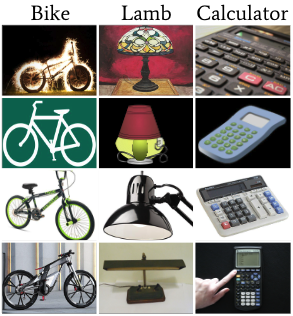
(c) OfficeHome

Figure 2: Image samples from the multi-domain DG evaluation datasets. Each figure visualizes the domain variations (rows) for different classes (columns) . Note that PACS and OfficeHome express significantly more distinguishable domain variations than VLCS.

We now describe the experimental set-up, our code will soon be released in the supplementary material along with additional details to reproduce our results, in App A.1. Additional results are presented in App A.5.

5.1 Datasets

PACS (Li et al., 2017a) is a 9,991-image dataset consisting of four domains corresponding to four different image styles: photo (P), art-painting (A), cartoon (C) and sketch (S). Each of the four domains hold seven object categories: dog, elephant, giraffe, guitar, horse, house and person.

VLCS (Fang et al., 2013) is a 10,729-image dataset consisting of four domains corresponding to four different datasets: VOC2007 (V), LabelMe (L), Caltech101 (C) and SUN09 (S). Each of the four domains hold five object categories: bird, car, chair, dog and person.

OfficeHome (Venkateswara et al., 2017) is a 15,588-image dataset consisting of images of everyday objects organized into four domains; art-painting, clip-art, images without backgrounds and real-world photos. Each of the domains holds 65 object categories typically found in offices and homes.

We selected these three datasets to analyze algorithm performance on for different 1) domain-variation types and 2) target class sizes. Namely, while the PACS (Fig. 2(b)) and OfficeHome (Fig. 2(c)) datasets share similar style-based domain-variations, there is a  10x difference in class size (7 and 65 respectively). Furthermore, although VLCS (Fig. 2(a)) and PACS have similar class sizes (5 and 7 respectively), VLCS expresses less distinguishable domain-variations.

5.2 Defining shared-class distribution settings

We define two shared-class distribution settings – Low and High – denoting the relative number of shared classes $|\mathcal{Y}_{S}|$ with respect to the total $|\mathcal{Y}_{T}|$ (refer to Table 3). For each setting $\mathcal{Y}_{L}$ and $\mathcal{Y}_{S}$ classes were randomly selected and assigned round-robin to each source-domain $\mathcal{S}$. $\mathcal{Y}_{S}$ classes are randomly assigned round-robin to $|\mathcal{S}|-1$ source-domains (i.e. no $\mathcal{Y}_{S}$ class is in all source-domains).

Table 1: Domain-shared ($\mathcal{Y}_{S}$) class sizes with the corresponding domain-linked ($\mathcal{Y}_{L}$) classes for each dataset and shared-class distribution setting. The left table outlines the $\mathcal{Y}_{S}$ class size with respect to the total $\mathcal{Y}_{T}$ class set. The right table displays the specific domain-linked $\mathcal{Y}_{L}$ classes for future reference. In the Low setting $\sim\nicefrac{{1}}{{3}}$ of the classes are domain-shared; $\sim\nicefrac{{2}}{{3}}$ in the High setting.

	$|\mathcal{Y}_{S}|/|\mathcal{Y}_{T}|$
Setting	PACS	OfficeHome	VLCS
Low	3/7	25/65	2/5
High	5/7	50/65	4/5

$\mathcal{Y}_{L}$
PACS	OfficeHome	VLCS
{0,1,3,5,6}	{0-13, 30-34, 44-64}	{0,1,4}
{1,6}	{0-4, 44-64}	{1}

5.3 Baseline algorithms

We compare our method (FOND) with existing methods for domain generalization: the naive Empirical Risk Minimization (ERM), the popular distribution-alignment technique CORAL (Sun and Saenko, 2016), contrastive methods SelfReg (Kim et al., 2021) and CAD (Ruan et al., 2022), meta-learning baseline ARM (Zhang et al., 2020) and MLDG (Li et al., 2017b) and the theoretical adversarial meta-learner Transfer (Zhang et al., 2021).

5.4 Model selection and evaluation

To standardize the model selection strategy across evaluated methods we based our experimental setup on the thorough domain generalization test-bed, DomainBed (Gulrajani and Lopez-Paz, 2021). Refer to the Appendix for details about the implementation (App. A.1), hyper-parameter search (App. A.2), and training-domain validation model selection (App. A.3).

Evaluation metrics for all experiments are class-averaged $\mathcal{Y}_{L}$ and $\mathcal{Y}_{S}$ classification accuracy’s because we are specifically interested in the ability for algorithms to transfer their domain generalizable representations from $\mathcal{Y}_{S}$ to $\mathcal{Y}_{L}$ classes.

Standard error bars in our experiments arise from repeating the entire model selection and hyper-parameter search for each dataset, algorithm and shared-class distribution three times. We report the mean algorithm performance over these repetitions. This allows the error bars to communicate performance stability in the algorithms.

5.5 Results

Table 2: Results on $\mathcal{Y}_{L}$ class accuracy evaluated on PACS, VLCS and OfficeHome for the Low and High shared-class distribution settings. FOND and variants significantly outperform all baselines during the High setting with top-3 performance on Low and best performance overall.

		Datasets
Setting	Algorithm	VLCS	PACS	OfficeHome	Average
Low	ERM	50.7 $\pm$ 1.0	36.5 $\pm$ 0.5	38.5 $\pm$ 0.4	41.9
	CORAL	45.5 $\pm$ 1.6	33.3 $\pm$ 0.8	40.7 $\pm$ 0.2	39.8
	MLDG	50.8 $\pm$ 2.0	38.0 $\pm$ 0.1	38.1 $\pm$ 0.1	42.3
	ARM	47.7 $\pm$ 0.9	36.8 $\pm$ 1.3	39.0 $\pm$ 0.1	41.2
	SelfReg	46.6 $\pm$ 1.2	32.4 $\pm$ 0.4	40.0 $\pm$ 0.3	39.6
	CAD	45.5 $\pm$ 1.5	33.0 $\pm$ 0.9	36.9 $\pm$ 1.2	38.5
	Transfer	48.3 $\pm$ 0.6	36.4 $\pm$ 1.8	38.1 $\pm$ 0.3	40.9
	FOND	48.0 $\pm$ 0.4	35.3 $\pm$ 1.2	40.3 $\pm$ 0.3	41.2
	FOND$\backslash$F	48.5 $\pm$ 1.0	35.3 $\pm$ 0.5	40.6 $\pm$ 0.6	41.5
	FOND$\backslash$FB	50.0 $\pm$ 0.2	33.2 $\pm$ 0.5	41.0 $\pm$ 0.5	41.4
	FOND$\backslash$FBA	46.6 $\pm$ 1.0	35.4 $\pm$ 1.2	41.0 $\pm$ 0.4	41.0
High	ERM	51.8 $\pm$ 3.3	13.7 $\pm$ 1.8	37.5 $\pm$ 0.6	34.3
	CORAL	49.8 $\pm$ 4.2	13.7 $\pm$ 1.0	38.9 $\pm$ 0.2	34.1
	MLDG	45.2 $\pm$ 3.4	13.8 $\pm$ 0.5	37.4 $\pm$ 0.7	32.1
	ARM	49.0 $\pm$ 1.4	16.2 $\pm$ 2.9	38.4 $\pm$ 0.2	34.5
	SelfReg	41.9 $\pm$ 0.2	13.4 $\pm$ 1.2	39.5 $\pm$ 0.6	31.6
	CAD	51.7 $\pm$ 5.8	13.1 $\pm$ 0.7	36.4 $\pm$ 1.4	33.7
	Transfer	48.9 $\pm$ 3.0	16.0 $\pm$ 1.6	36.8 $\pm$ 0.2	33.9
	FOND	72.1 $\pm$ 3.5	19.1 $\pm$ 0.6	40.6 $\pm$ 0.4	43.9
	FOND$\backslash$F	51.7 $\pm$ 6.0	17.5 $\pm$ 1.4	40.8 $\pm$ 0.6	36.7
	FOND$\backslash$FB	44.0 $\pm$ 2.3	15.4 $\pm$ 0.6	41.7 $\pm$ 0.7	33.7
	FOND$\backslash$FBA	51.3 $\pm$ 2.8	17.3 $\pm$ 1.3	39.1 $\pm$ 0.5	35.9
Low/High Average	ERM	51.3 $\pm$ 2.2	25.6 $\pm$ 1.4	38.0 $\pm$ 0.2	38.3
	CORAL	47.7 $\pm$ 2.9	23.5 $\pm$ 0.9	39.8 $\pm$ 0.2	37.0
	MLDG	48.0 $\pm$ 2.7	25.9 $\pm$ 1.4	37.8 $\pm$ 0.4	37.2
	ARM	48.4 $\pm$ 1.2	26.5 $\pm$ 2.1	38.7 $\pm$ 0.2	37.9
	SelfReg	44.3 $\pm$ 0.7	22.9 $\pm$ 1.4	39.8 $\pm$ 0.5	35.6
	CAD	48.6 $\pm$ 3.7	23.1 $\pm$ 0.8	36.7 $\pm$ 1.3	36.1
	Transfer	48.6 $\pm$ 1.8	26.2 $\pm$ 1.7	37.5 $\pm$ 0.3	37.4
	FOND	60.1 $\pm$ 2.0	27.2 $\pm$ 0.9	40.5 $\pm$ 0.4	42.6
	FOND$\backslash$F	50.1 $\pm$ 3.5	26.4 $\pm$ 1.0	40.7 $\pm$ 0.6	39.1
	FOND$\backslash$FB	47.0 $\pm$ 1.3	24.3 $\pm$ 0.6	41.4 $\pm$ 0.6	37.6
	FOND$\backslash$FBA	49.0$\pm$ 1.9	26.4 $\pm$ 1.3	40.1 $\pm$ 0.5	38.5

$\mathcal{Y}_{L}$ Accuracy

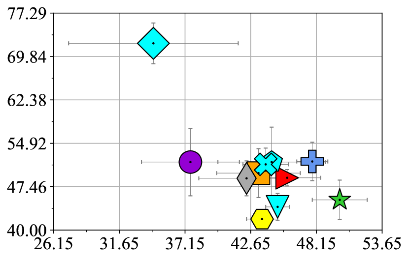
(a) VLCS-High

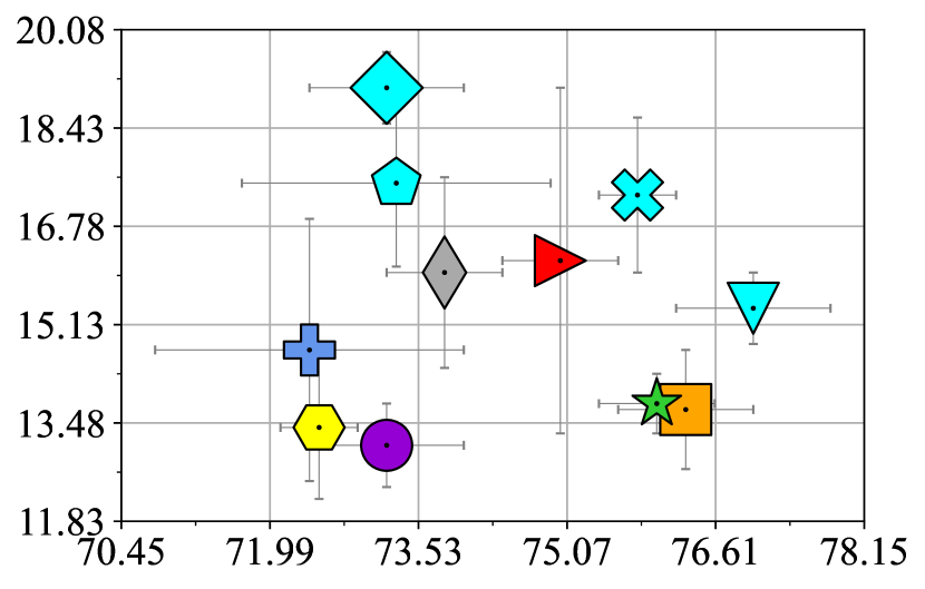
(b) PACS-High

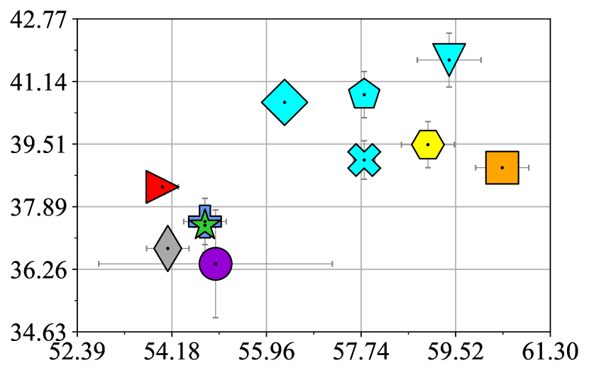
(c) OfficeHome-High

$\mathcal{Y}_{S}$ Accuracy

Figure 3: Visualizing $\mathcal{Y}_{L}$ and $\mathcal{Y}_{S}$ performance trade-offs on the High shared-class distribution setting. Our method outperforms all baselines on $\mathcal{Y}_{L}$ classes with more competitive $\mathcal{Y}_{S}$ class performance as the total number of target classes increases (left to right). Additional plots in App. A.5.

Dimension 1

(a) ERM source data (classes)

(b) ERM source data (domains)

(c) ERM target data (classes)

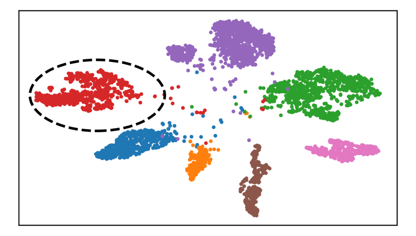
(d) ARM source data (classes)

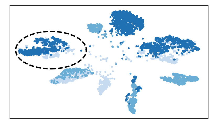
(e) ARM source data (domains)

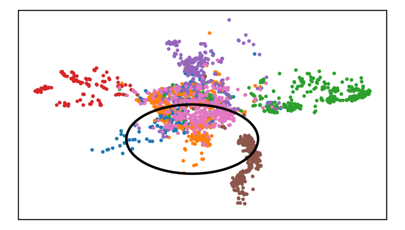
(f) ARM target data (classes)

(g) FOND source data (classes)

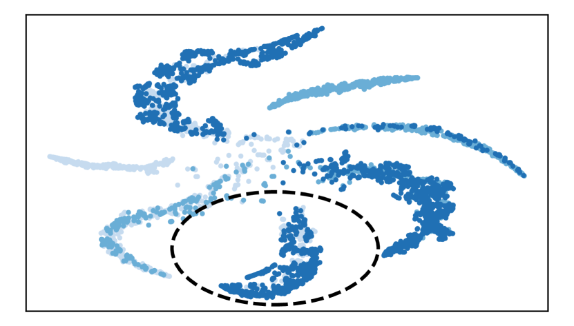
(h) FOND source data (domains)

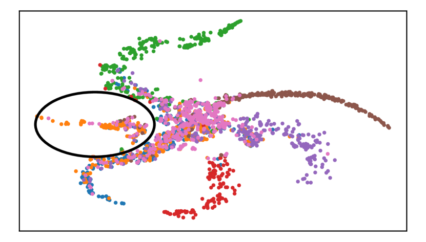
(i) FOND target data (classes)

Dimension 2

Figure 4: t-SNE latent $\mathbf{h}$ representation visualization for the PACS-High dataset. Each row visualizes the representations of the naive (ERM), top-performing-baseline (ARM) and our (FOND) algorithm. Source-domain (Photo, Art and Sketch) representations are colored by class and domain. Target-domain (Cartoon) representations are colored by class. We highlight domain-linked $\mathcal{Y}_{L}$ class generalization (solid circle) and domain-invariant learning (broken circle) in Sec. 5.6.

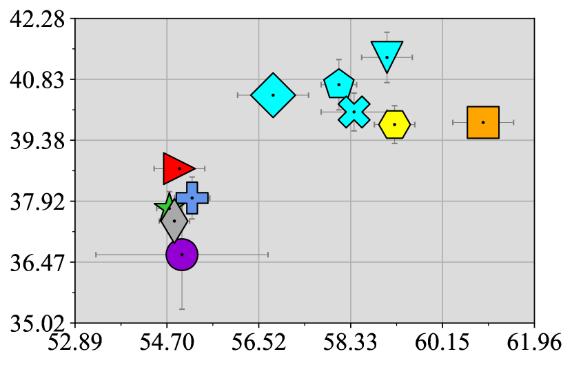
(a) OfficeHome-Average

(b) OfficeHome-High

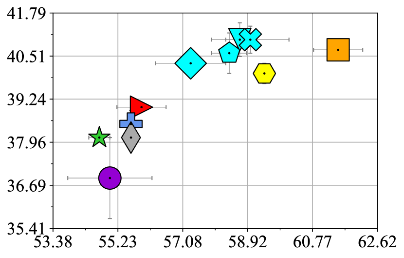
(c) OfficeHome-Low

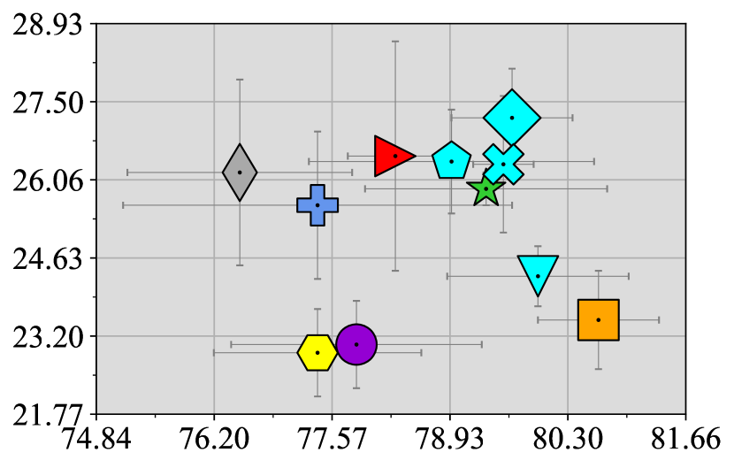
(d) PACS-Average

(e) PACS-High

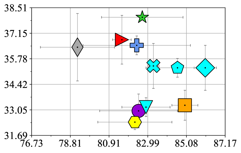
(f) PACS-Low

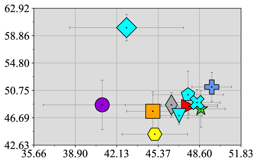
(g) VLCS-Average

(h) VLCS-High

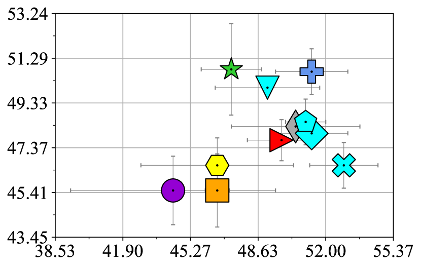
(i) VLCS-Low

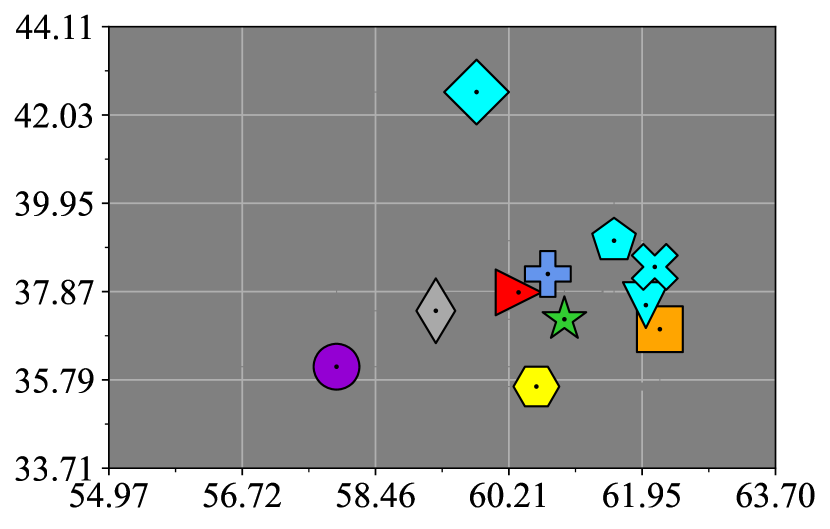
(j) Average-Average

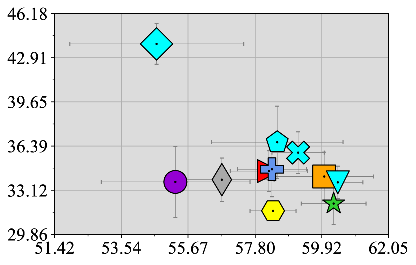
(k) Average-High

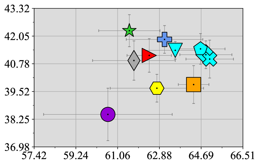
(l) Average-Low

Domain-Shared ($\mathcal{Y}_{S}$) Accuracy

Figure 6: Visualizing baseline and ablation algorithm accuracy between $\mathcal{Y}_{L}$ and $\mathcal{Y}_{S}$ classes across all datasets and shared-class settings. The white plots communicate accuracies for each dataset’s High and Low shared-class settings. The light-grey plots communicate average accuracies for each dataset (left-most column) and shared-class setting (bottom-row). The dark-grey plot (bottom-left) communicates the average accuracies across all datasets and shared-class settings. The exact values and standard error bars are displayed in Table 2.

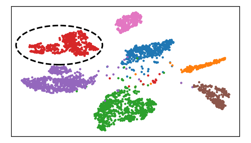
(a) Transfer source data (classes)

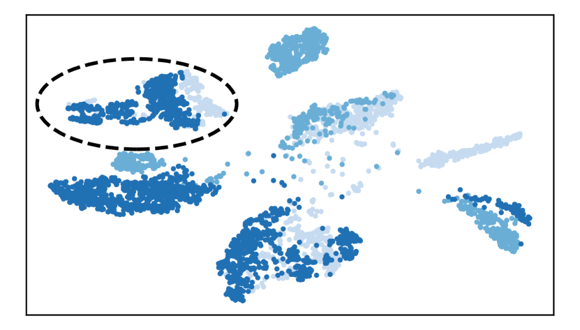
(b) Trans. source data (domains)

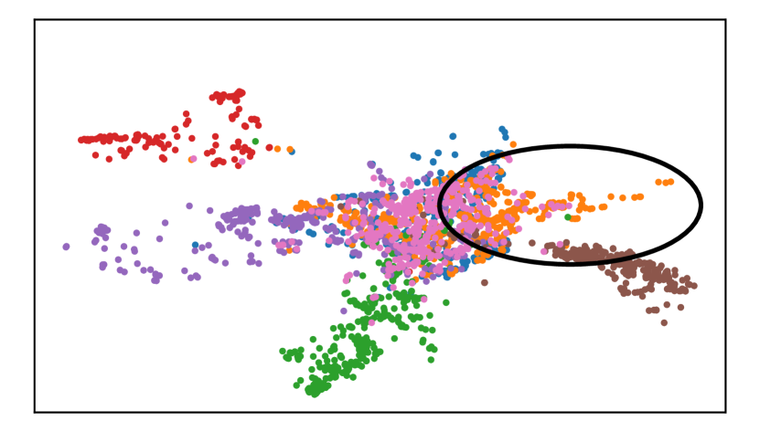
(c) Transfer target data (classes)

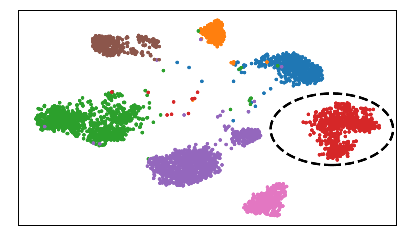
(d) CAD source data (classes)

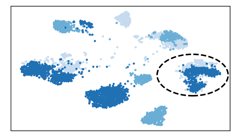
(e) CAD source data (domains)

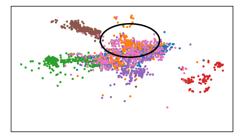
(f) CAD target data (classes)

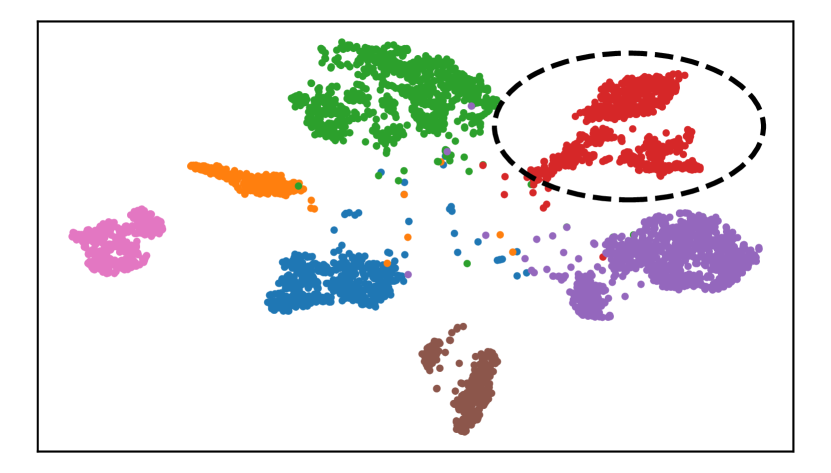
(g) MLDG source data (classes)

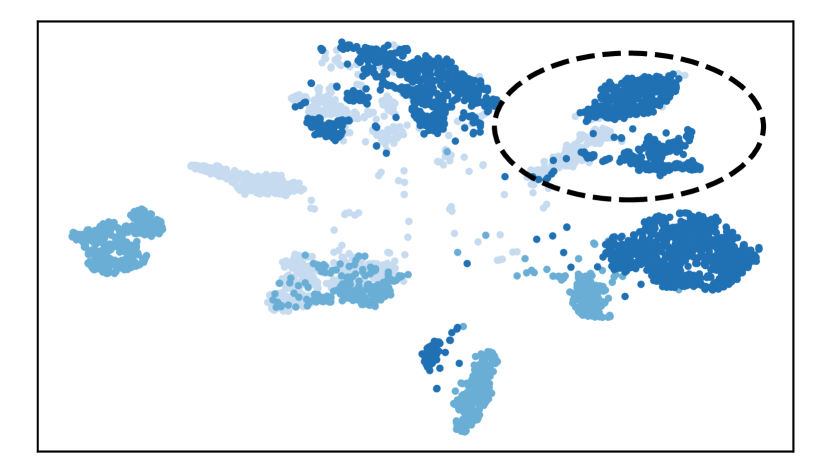
(h) MLDG source data (domains)

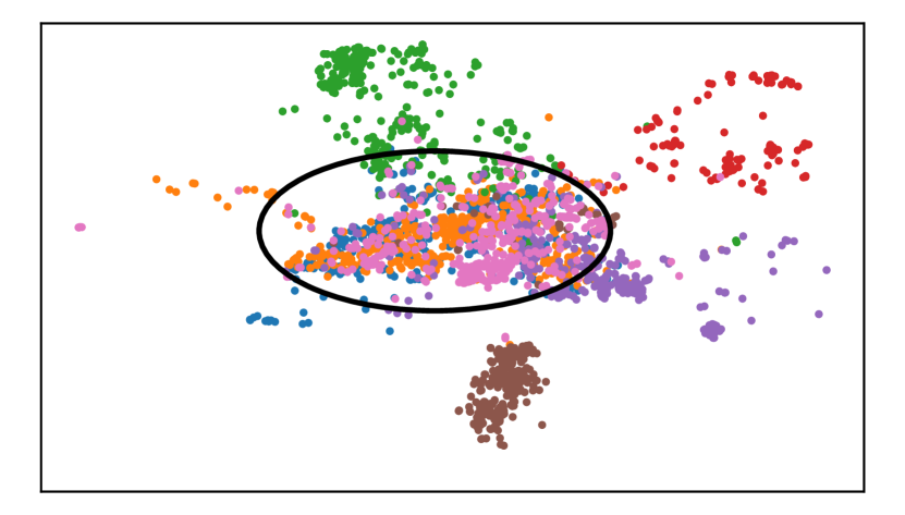
(i) MLDG target data (classes)

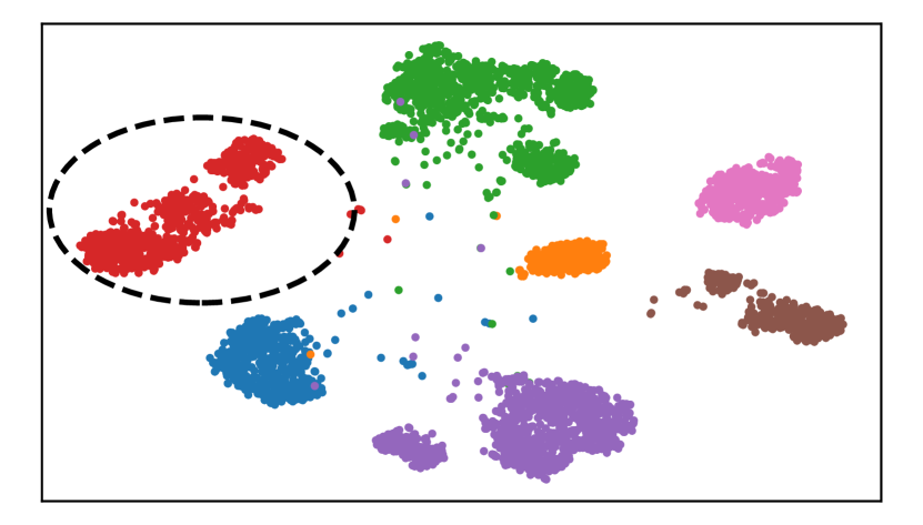
(j) SelfReg source data (classes)

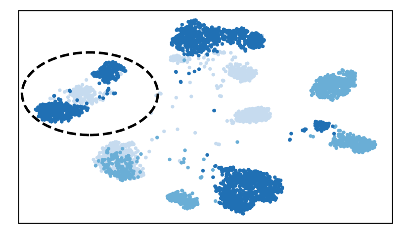
(k) Self. source data (domains)

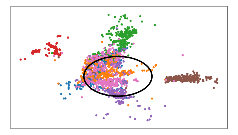
(l) SelfReg target data (classes)

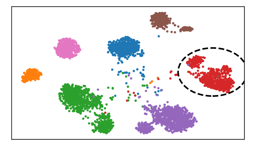
(m) COR. source data (classes)

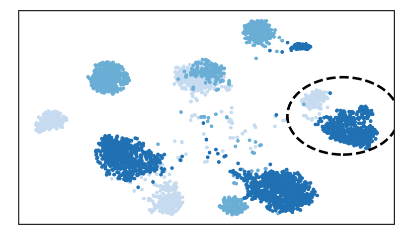
(n) COR. source data (domains)

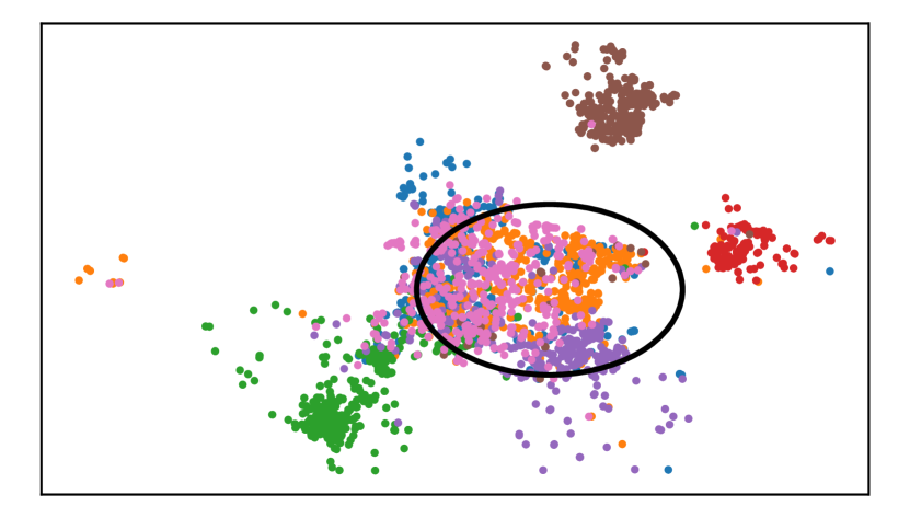
(o) CORAL target data (classes)

Dimension 2

Figure 7: Additional t-SNE latent representation visualization for the PACS-High dataset. Each row visualizes the additional representations of the baseline algorithms (i.e. Transfer, CAD, MLDG, SelfReg, CORAL). Source-domain (Photo, Art and Sketch) representations are colored by class and domain. Target-domain (Cartoon) representations are colored by class. Refer to the analysis of the domain-linked $\mathcal{Y}_{L}$ class generalization (solid circle) and domain-invariant learning evidence (broken circle) found in Sec. 5.6.

In this section we analyze the domain-linked $\mathcal{Y}_{L}$ class generalization performances in Table 2 and visualize the $\mathcal{Y}_{L}$ and $\mathcal{Y}_{S}$ class performance trade-offs in Fig. 6. Additionally, we also compare the learned representation via the t-SNE (van der Maaten and Hinton, 2008) plots capture in Fig. 7.

Our method consistently outperforms all baselines on all datasets during the High shared-class distribution setting. In Table 2 FOND achieves performance improvements on PACS (+2.9%), VLCS (+20.3%), and OfficeHome (+1.1%). Although MLDG and ERM outperform FOND in the Low setting (+1.1% and +0.7% on average), FOND outperforms all baselines on average. Omitting the fairness objective (i.e. FOND$\backslash$F) still outperforms all baselines on the High setting by +2.2% including the variants omitting $\alpha$ and/or $\beta$ (i.e. FOND$\backslash$FB, FOND$\backslash$FBA). This affirms our hypothesis that targeting specific pairwise relationships with $\alpha$ and $\beta$ is conducive for increasing $\mathcal{Y}_{L}$ generalizability. We also observe (Fig. 6(h)) that our method’s strong High-VLCS $\mathcal{Y}_{L}$ performance trades-off $\mathcal{Y}_{S}$ performance.

Fairness is the most effective regularizer when domain-variations within a dataset are indistinct. We compare between the distinguishable style-based domain-variations in PACS/OfficeHome versus the subtle and indistinct domain-variations in VLCS (Fig. 2). In Table 2 when averaging across Low and High on VLCS our method outperforms all baselines (+8.8%). Interestingly, the domain-naive ERM algorithm outperforms the rest of the domain-aware baselines by +2.7%. Additionally, among FOND variants, fairness is responsible for the strong VLCS-High performance. We believe that since domain-naive regularizers do not assume distinguishable domain-variations they yield better performance on VLCS. This may also additionally benefit the domain-naive fairness over the domain-aware $\alpha$ and $\beta$ on VLCS whereas we see the performance difference drop on the PACS and OffiHome dataset. However, our method still outperforms all other methods on the more distinguishable domain variations (+3.5%/+0.7% on PACS-High/PACS-Average, and +1.1%/+0.7% on OfficeHome-High/OfficeHome-Average). We observe that with distinct domain-variations, the domain-aware regularization’s of meta-learners (ARM, Transfer) on PACS (Fig. 6(e)) and feature-alignment methods (CORAL, SelfReg) on OfficeHome (Fig. 6(b)) outperform ERM for both $\mathcal{Y}_{L}$ and $\mathcal{Y}_{S}$ classes.

Increasing the total number of domain-shared classes observed improves domain-linked generalization. In Table 2 and Fig. 6(b) feature-alignment methods (SelfReg and CORAL) consistently outperform other baselines on the 65-class OfficeHome dataset. Meta-learning algorithms (Transfer, MLDG and ARM) outperform other baselines on average in the lower class-size datasets PACS/VLCS; ARM and Transfer both yield a $\geq 2\%$ improvement in PACS-High; MLDG is the top-performing baseline in the Low setting for both PACS and VLCS. However, in the High setting FOND outperforms baselines regardless off class-size. In addition, during the Low shared-class setting, FOND yields its smallest performance difference with the top-performing baselines during the 65-class OfficeHome dataset (-0.4% versus -2.8% and -2.7% in VLCS and PACS respectively). This communicates that increasing $\mathcal{Y}_{L}$ performance benefits from observing a larger number of domain-shared classes even in a relatively low shared-class distribution setting.

5.6 Visualizing learned latent representations

In Fig. 7 we visualize latent representations from the PACS-High dataset via t-SNE plots (van der Maaten and Hinton, 2008). To gain insight on our method’s strong performance during the High shared-class distribution setting we analyze the representations learned by ERM (naive-baseline), ARM (top-performing-baseline) and FOND (top-performing-method). On source-domain data the ERM class-colored clusters are also distinctly sub-clustered by domain (e.g. broken circle in Fig. 4(a) and Fig. 4(b)). Whereas ARM (Fig.  4(d) and Fig. 4(e)) and FOND (Fig. 4(g) and Fig. 4(h)) demonstrate more domain-invariant representations since their classes are not as distinctly clustered by domain. For domain-linked $\mathcal{Y}_{L}$ class samples, FOND (e.g. solid circle in Fig. 4(i)) yields more generalizable representations than ARM (Fig. 4(f)) and ERM (Fig. 4(c)). While all methods struggle on the pink class, FOND empirically maintains top performance.

6 Discussion

Domain generalization (DG) in real-world settings often suffers from data scarcity arising from classes which are only observed in certain domains, i.e. they are domain-linked. While efforts in the area have focused on improving the overall accuracy, these works, to the best of our knowledge, have overlooked the performance on such underrepresented classes, which can lead to critical failures in the real-world. Motivated from these observations, we focused on improving the out-of-distribution generalization for such domain-linked classes by aiming to transfer domain-invariant knowledge from classes which are shared between source-domains (domain-shared). Consequently, we proposed FOND; the first method for domain-linked DG which promotes fairness between domain-linked and shared classes, and leverages contrastive learning to learn domain invariant representations. Through extensive experimentation and visualizations of the learned representations we arrive at a key insight: FOND consistently outperforms baselines given a sufficient number for domain-shared classes to learn from. The ability to leverage knowledge from domain-shared classes to accomplish state-of-the-art results for domain-linked ones opens tremendous possibilities for real-world DG, stimulating domain generalization research for real-world data-scarce domains.

Limitations and future work. One of the key limitations is that our method does not perform well when observing very few domain-shared $\mathcal{Y}_{L}$ classes is a general lack of domain-shared data, e.g., during the Low share-class distribution setting. This is a problem across all methods, which seem to struggle to beat the naive ERM baseline. Another limitation is that DG methods in general are not agnostic to source-domain identities during training, and therefore it implicitly assumes that domains are disparate. As seen from our experiments, this can be disadvantageous for learning (and beating ERM) in cases where domains may not be very different (e.g. VLCS). Both cases provide strong motivation to fundamentally rethink the DG-specific algorithmic biases and assumptions.

Broader impacts. Our fairness objective is conditioned on a class being represented in multiple domains, which in the real-world may result from representation inequalities of protected attributes and/or classes which are only observed in certain domains (or rarely observed in others). Therefore, careful consideration is required when deploying fairness based DG research since they could make decisions that unfairly impact specific groups. This work demonstrates how we can begin to think about these challenging tasks. On the computation from, domain generalization research is computationally heavy since it requires multiple validation cycles for each dataset, algorithm, hyper-parameters search space and shared-class distribution setting. Therefore, as we expand DG research we need to improve ML resource efficiency to both increases its accessibility and reduce negative environmental consequences.

Appendix A Appendix

A.1 Implementation details

For consistency, all algorithms have a fine-tuned ResNet-18 backbone (He et al., 2015) pre-trained on ImageNet (Deng et al., 2009). Specifically, we replace the final (softmax) layer, insert a dropout layer and then fine-tune the entire network. Since minibatches from different domains follow different distributions, batch normalization degrades domain generalization algorithms (Seo et al., 2019). Therefore, we freeze all batch normalization layers before fine-tuning. Additionally, the training data augmentations are: random size crops and aspect ratios, resizing to 224 × 224 pixels, random horizontal flips, random color jitter, and random gray-scaling. Our experiments ran on different GPUs: NVIDIA RTXA600, NVIDIA GeForce RTX2080.

A.2 Hyper-parameter search

For each algorithm we perform five random search attempts over a joint distributions of all their hyper-parameters. The performance of each hyper-parameter is evaluated using the strategy outlined in App. A.3. This is repeated for each of the five sets of hyper-parameters and the set maximizing the average domain-linked $\mathcal{Y}_{L}$ accuracy is selected. This search is performed for across three different seeds where all hyper-parameters are optimized anew for each algorithm, dataset and partial-overlap setting.

A.3 Training-domain validation

Given $K$ domains, we train $K$ models, sharing the same hyper-parameters $\theta$, but each model holds a different domain out. During the training of each model, 80% of the training data from each domain is used for training and the other 20% is used to determine the version that will be evaluated. We evaluate each model on its held-out domain data, and average the $\mathcal{Y}_{L}$ accuracy of these $K$ models over their held-out domains. This provides us with an estimate of the quality of a given set of hyper-parameters. This strategy was chosen because it aligns with the goal of maximizing expected performance under out-of-distribution domain-variation without picking the model using the out-of-distribution data. The $\mathcal{Y}_{L}$ accuracy performance across held-out domains and final averages for each dataset, algorithm and partial-overlap setting are displayed in Table 2.

A.4 Model architecture

In this section we describe the FOND architecture components and outline the intermediate latent representations that are used for our learning objectives.

• The Feature Extraction Network, $F(.)$, takes a training input sample $\mathbf{x}\in\mathcal{S}$ and generates a representation vector, $\mathbf{h}=F(\mathbf{x})\in\mathbb{R}^{d_{F}}$ where $d_{F}=512$.

• The Projection Network, $P(.)$, takes the representation vector $\mathbf{h}$ and non-linearly projects it to a lower-dimensional vector $\mathbf{z}=P(\mathbf{h})\in\mathbb{R}^{d_{P}}$ where $d_{P}=256$. Additionally, the projection vector is normalized $||\mathbf{z}||=1$. These projections are used for FONDs‘’s contrastive learning objective (Eq. 2).

• The Classification Network, $G(.)$, performs the image classification downstream task with the representations generated by $F(.)$, i.e., $\mathbf{h}\in\mathbb{R}^{d_{F}}$. The network’s output is a vector of dimension $|\mathcal{Y}_{T}|$ denoting the softmax label probabilities of the input $\mathbf{x}$.

A.5 Additional results

$\mathcal{Y}_{L}$ Accuracy

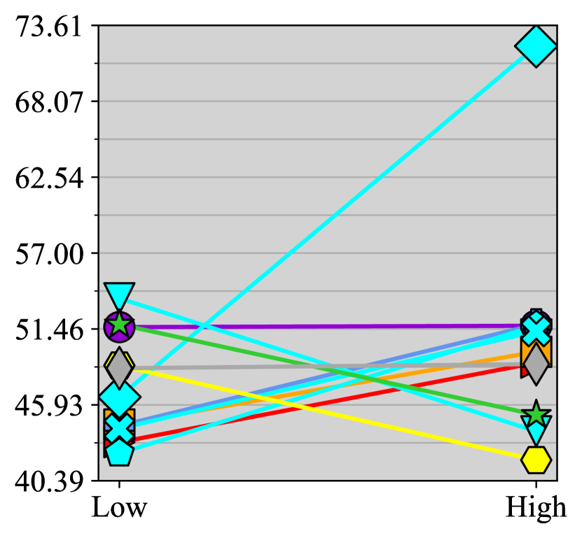
(a) VLCS

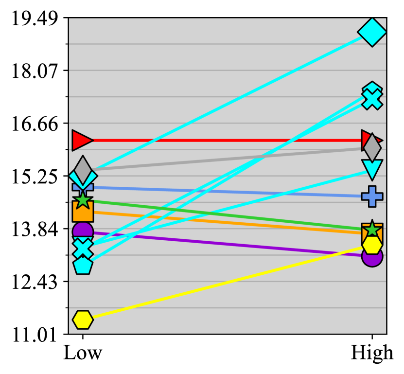
(b) PACS

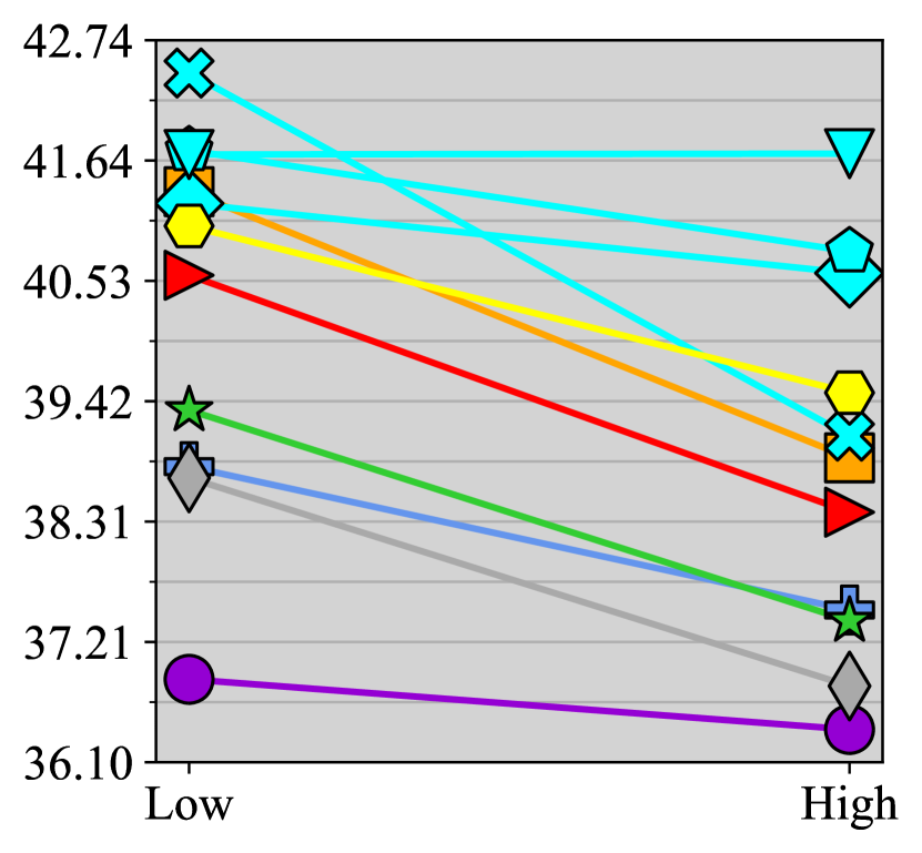
(c) OfficeHome

Shared-Class Distribution Setting

Figure 5: Tracking domain-linked $\mathcal{Y}_{L}$ performances for classes in both Low and High shared-class distribution settings. These results demonstrate how the domain-linked class performance changes when algorithms are presented with additional domain-shared classes (i.e. transition from Low to High). For the small class-size datasets (PACS & VLCS) FOND yields consistently larger $\mathcal{Y}_{L}$ performance improvements when observing more domain-shared $\mathcal{Y}_{S}$ classes. Interestingly, all algorithms suffer $\mathcal{Y}_{L}$ accuracy drops on the 65-class OfficeHome dataset. We note that for small class-size datasets (PACS & VLCS), the transition from Low to High entails making only 2 domain-linked classes become domain-shared (by introducing data from multiple domains. However for OfficeHome, 25 classes become domain-shared resulting in algorithms prioritizing the larger corpus of domain-shared classes. Additionally, since PACS, VLCS, and OfficeHome have similar dataset sizes, OfficeHome home has $\sim$10x less samples per domain-linked $\mathcal{Y}_{L}$ class.

Table 3: Domain-shared ($\mathcal{Y}_{S}$) class sizes with the corresponding domain-linked ($\mathcal{Y}_{L}$) classes for each dataset and shared-class distribution setting. The left table outlines the $\mathcal{Y}_{S}$ class size with respect to the total $\mathcal{Y}_{T}$ class set. The right table displays the specific domain-linked $\mathcal{Y}_{L}$ classes for future reference. In the Low setting $\sim\nicefrac{{1}}{{3}}$ of the classes are domain-shared; $\sim\nicefrac{{2}}{{3}}$ in the High setting.

	$|\mathcal{Y}_{S}|/|\mathcal{Y}_{T}|$
Setting	PACS	OfficeHome	VLCS
Low	3/7	25/65	2/5
High	5/7	50/65	4/5

$\mathcal{Y}_{L}$
PACS	OfficeHome	VLCS
{0,1,3,5,6}	{0-13, 30-34, 44-64}	{0,1,4}
{1,6}	{0-4, 44-64}	{1}

Domain-Linked ($\mathcal{Y}_{L}$) Accuracy

Dimension 1

References

- Albuquerque et al. [2019] Isabela Albuquerque, João Monteiro, Tiago H. Falk, and Ioannis Mitliagkas. Adversarial target-invariant representation learning for domain generalization. ArXiv, abs/1911.00804, 2019.
- Anoosheh et al. [2017] Asha Anoosheh, Eirikur Agustsson, Radu Timofte, and Luc Van Gool. Combogan: Unrestrained scalability for image domain translation. 2018 IEEE/CVF Conference on Computer Vision and Pattern Recognition Workshops (CVPRW), pages 896–8967, 2017.
- Ataabadi et al. [2022] Parvin Esmaeili Ataabadi, Behzad Soleimani Neysiani, Mohammad Zahiri Nogorani, and Nazanin Mehraby. Semi-supervised medical insurance fraud detection by predicting indirect reductions rate using machine learning generalization capability. In 2022 8th International Conference on Web Research (ICWR), pages 176–182, 2022. doi: 10.1109/ICWR54782.2022.9786251.
- Chen et al. [2021] Irene Y. Chen, Emma Pierson, Sherri Rose, Shalmali Joshi, Kadija Ferryman, and Marzyeh Ghassemi. Ethical machine learning in healthcare. Annual Review of Biomedical Data Science, 4(1):123–144, 2021. doi: 10.1146/annurev-biodatasci-092820-114757. URL https://doi.org/10.1146/annurev-biodatasci-092820-114757.
- Chen et al. [2020] Ting Chen, Simon Kornblith, Mohammad Norouzi, and Geoffrey E. Hinton. A simple framework for contrastive learning of visual representations. ArXiv, abs/2002.05709, 2020.
- Deng et al. [2009] Jia Deng, Wei Dong, Richard Socher, Li-Jia Li, K. Li, and Li Fei-Fei. Imagenet: A large-scale hierarchical image database. 2009 IEEE Conference on Computer Vision and Pattern Recognition, pages 248–255, 2009.
- Fang et al. [2013] Chen Fang, Ye Xu, and Daniel N. Rockmore. Unbiased metric learning: On the utilization of multiple datasets and web images for softening bias. 2013 IEEE International Conference on Computer Vision, pages 1657–1664, 2013.
- Gong et al. [2018] Rui Gong, Wen Li, Yuhua Chen, and Luc Van Gool. Dlow: Domain flow for adaptation and generalization. 2019 IEEE/CVF Conference on Computer Vision and Pattern Recognition (CVPR), pages 2472–2481, 2018.
- Gulrajani and Lopez-Paz [2021] Ishaan Gulrajani and David Lopez-Paz. In search of lost domain generalization. In International Conference on Learning Representations, 2021. URL https://openreview.net/forum?id=lQdXeXDoWtI.
- He et al. [2015] Kaiming He, X. Zhang, Shaoqing Ren, and Jian Sun. Deep residual learning for image recognition. 2016 IEEE Conference on Computer Vision and Pattern Recognition (CVPR), pages 770–778, 2015.
- Hu et al. [2019] Shoubo Hu, Kun Zhang, Zhitang Chen, and Lai-Wan Chan. Domain generalization via multidomain discriminant analysis. Uncertainty in artificial intelligence : proceedings of the … conference. Conference on Uncertainty in Artificial Intelligence, 35, 2019.
- Huang and Belongie [2017] Xun Huang and Serge J. Belongie. Arbitrary style transfer in real-time with adaptive instance normalization. 2017 IEEE International Conference on Computer Vision (ICCV), pages 1510–1519, 2017.
- Huang et al. [2020] Zeyi Huang, Haohan Wang, Eric P Xing, and Dong Huang. Self-challenging improves cross-domain generalization. In Computer Vision–ECCV 2020: 16th European Conference, Glasgow, UK, August 23–28, 2020, Proceedings, Part II 16, pages 124–140. Springer, 2020.
- Khosla et al. [2020] Prannay Khosla, Piotr Teterwak, Chen Wang, Aaron Sarna, Yonglong Tian, Phillip Isola, Aaron Maschinot, Ce Liu, and Dilip Krishnan. Supervised contrastive learning. ArXiv, abs/2004.11362, 2020.
- Kilbertus et al. [2017] Niki Kilbertus, Mateo Rojas Carulla, Giambattista Parascandolo, Moritz Hardt, Dominik Janzing, and Bernhard Schölkopf. Avoiding discrimination through causal reasoning. In I. Guyon, U. Von Luxburg, S. Bengio, H. Wallach, R. Fergus, S. Vishwanathan, and R. Garnett, editors, Advances in Neural Information Processing Systems, volume 30. Curran Associates, Inc., 2017. URL https://proceedings.neurips.cc/paper_files/paper/2017/file/f5f8590cd58a54e94377e6ae2eded4d9-Paper.pdf.
- Kim et al. [2021] Daehee Kim, Seunghyun Park, Jinkyu Kim, and Jaekoo Lee. Selfreg: Self-supervised contrastive regularization for domain generalization. 2021 IEEE/CVF International Conference on Computer Vision (ICCV), pages 9599–9608, 2021.
- Li et al. [2017a] Da Li, Yongxin Yang, Yi-Zhe Song, and Timothy M. Hospedales. Deeper, broader and artier domain generalization. 2017 IEEE International Conference on Computer Vision (ICCV), pages 5543–5551, 2017a.
- Li et al. [2017b] Da Li, Yongxin Yang, Yi-Zhe Song, and Timothy M. Hospedales. Learning to generalize: Meta-learning for domain generalization. CoRR, abs/1710.03463, 2017b. URL http://arxiv.org/abs/1710.03463.
- Li et al. [2018] Haoliang Li, Sinno Jialin Pan, Shiqi Wang, and Alex Chichung Kot. Domain generalization with adversarial feature learning. 2018 IEEE/CVF Conference on Computer Vision and Pattern Recognition, pages 5400–5409, 2018.
- Makhlouf et al. [2021] Karima Makhlouf, Sami Zhioua, and Catuscia Palamidessi. Machine learning fairness notions: Bridging the gap with real-world applications. Information Processing & Management, 58(5):102642, 2021. ISSN 0306-4573. doi: https://doi.org/10.1016/j.ipm.2021.102642. URL https://www.sciencedirect.com/science/article/pii/S0306457321001321.
- Mancini et al. [2020] Massimiliano Mancini, Zeynep Akata, Elisa Ricci, and Barbara Caputo. Towards recognizing unseen categories in unseen domains. ArXiv, abs/2007.12256, 2020.
- Motiian et al. [2017] Saeid Motiian, Marco Piccirilli, Donald A. Adjeroh, and Gianfranco Doretto. Unified deep supervised domain adaptation and generalization. 2017 IEEE International Conference on Computer Vision (ICCV), pages 5716–5726, 2017.
- Nguyen et al. [2021a] A. Tuan Nguyen, Toan Tran, Yarin Gal, and Atilim Gunes Baydin. Domain invariant representation learning with domain density transformations. In M. Ranzato, A. Beygelzimer, Y. Dauphin, P.S. Liang, and J. Wortman Vaughan, editors, Advances in Neural Information Processing Systems, volume 34, pages 5264–5275. Curran Associates, Inc., 2021a. URL https://proceedings.neurips.cc/paper/2021/file/2a2717956118b4d223ceca17ce3865e2-Paper.pdf.
- Nguyen et al. [2021b] Van-Anh Nguyen, Tuan Nguyen, Trung Le, Quan Hung Tran, and Dinh Q. Phung. Stem: An approach to multi-source domain adaptation with guarantees. 2021 IEEE/CVF International Conference on Computer Vision (ICCV), pages 9332–9343, 2021b.
- Peng et al. [2019] Xingchao Peng, Qinxun Bai, Xide Xia, Zijun Huang, Kate Saenko, and Bo Wang. Moment matching for multi-source domain adaptation. 2019 IEEE/CVF International Conference on Computer Vision (ICCV), pages 1406–1415, 2019.
- Pham et al. [2023] Thai-Hoang Pham, Xueru Zhang, and Ping Zhang. Fairness and accuracy under domain generalization. In The Eleventh International Conference on Learning Representations, 2023. URL https://openreview.net/forum?id=jBEXnEMdNOL.
- Piva et al. [2023] Fabrizio J. Piva, Daan de Geus, and Gijs Dubbelman. Empirical generalization study: Unsupervised domain adaptation vs. domain generalization methods for semantic segmentation in the wild. In Proceedings of the IEEE/CVF Winter Conference on Applications of Computer Vision (WACV), pages 499–508, January 2023.
- Ruan et al. [2022] Yangjun Ruan, Yann Dubois, and Chris J. Maddison. Optimal representations for covariate shift. CoRR, abs/2201.00057, 2022. URL https://arxiv.org/abs/2201.00057.
- Seo et al. [2019] Seonguk Seo, Yumin Suh, Dongwan Kim, Jongwoo Han, and Bohyung Han. Learning to optimize domain specific normalization for domain generalization. In European Conference on Computer Vision, 2019.
- Shankar et al. [2018] Shiv Shankar, Vihari Piratla, Soumen Chakrabarti, Siddhartha Chaudhuri, Preethi Jyothi, and Sunita Sarawagi. Generalizing across domains via cross-gradient training. ArXiv, abs/1804.10745, 2018.
- Shao et al. [2019] Rui Shao, Xiangyuan Lan, Jiawei Li, and Pong C Yuen. Multi-adversarial discriminative deep domain generalization for face presentation attack detection. In Proceedings of the IEEE/CVF conference on computer vision and pattern recognition, pages 10023–10031, 2019.
- Shorten and Khoshgoftaar [2019] Connor Shorten and Taghi M. Khoshgoftaar. A survey on image data augmentation for deep learning. Journal of Big Data, 6:1–48, 2019.
- Shu et al. [2021] Yang Shu, Zhangjie Cao, Chenyu Wang, Jianmin Wang, and Mingsheng Long. Open domain generalization with domain-augmented meta-learning. 2021 IEEE/CVF Conference on Computer Vision and Pattern Recognition (CVPR), pages 9619–9628, 2021.
- Somavarapu et al. [2020] Nathan Somavarapu, Chih-Yao Ma, and Zsolt Kira. Frustratingly simple domain generalization via image stylization. ArXiv, abs/2006.11207, 2020.
- Sun and Saenko [2016] Baochen Sun and Kate Saenko. Deep CORAL: correlation alignment for deep domain adaptation. CoRR, abs/1607.01719, 2016. URL http://arxiv.org/abs/1607.01719.
- Tobin et al. [2017] Joshua Tobin, Rachel Fong, Alex Ray, Jonas Schneider, Wojciech Zaremba, and P. Abbeel. Domain randomization for transferring deep neural networks from simulation to the real world. 2017 IEEE/RSJ International Conference on Intelligent Robots and Systems (IROS), pages 23–30, 2017.
- Tremblay et al. [2018] Jonathan Tremblay, Aayush Prakash, David Acuna, Mark Brophy, V. Jampani, Cem Anil, Thang To, Eric Cameracci, Shaad Boochoon, and Stan Birchfield. Training deep networks with synthetic data: Bridging the reality gap by domain randomization. 2018 IEEE/CVF Conference on Computer Vision and Pattern Recognition Workshops (CVPRW), pages 1082–10828, 2018.
- van der Maaten and Hinton [2008] Laurens van der Maaten and Geoffrey Hinton. Visualizing data using t-sne. Journal of Machine Learning Research, 9(86):2579–2605, 2008. URL http://jmlr.org/papers/v9/vandermaaten08a.html.
- Vapnik [2000] Vladimir Naumovich Vapnik. The nature of statistical learning theory. In Statistics for Engineering and Information Science, 2000.
- Venkateswara et al. [2017] Hemanth Venkateswara, Jose Eusebio, Shayok Chakraborty, and Sethuraman Panchanathan. Deep hashing network for unsupervised domain adaptation. In Proceedings of the IEEE Conference on Computer Vision and Pattern Recognition, pages 5018–5027, 2017.
- Volpi et al. [2018] Riccardo Volpi, Hongseok Namkoong, Ozan Sener, John C Duchi, Vittorio Murino, and Silvio Savarese. Generalizing to unseen domains via adversarial data augmentation. Advances in neural information processing systems, 31, 2018.
- Wang et al. [2021a] Jindong Wang, Cuiling Lan, Chang Liu, Yidong Ouyang, and Tao Qin. Generalizing to unseen domains: A survey on domain generalization. In International Joint Conference on Artificial Intelligence, 2021a.
- Wang et al. [2021b] Junchang Wang, Yang Li, Liyan Xie, and Yao Xie. Class-conditioned domain generalization via wasserstein distributional robust optimization. ArXiv, abs/2109.03676, 2021b.
- Wang et al. [2020] Zeyu Wang, Klint Qinami, Ioannis Christos Karakozis, Kyle Genova, Prem Nair, Kenji Hata, and Olga Russakovsky. Towards fairness in visual recognition: Effective strategies for bias mitigation. In Proceedings of the IEEE/CVF conference on computer vision and pattern recognition, pages 8919–8928, 2020.
- Yang et al. [2021] Fu-En Yang, Yuan-Chia Cheng, Zu-Yun Shiau, and Yu-Chiang Frank Wang. Adversarial teacher-student representation learning for domain generalization. In M. Ranzato, A. Beygelzimer, Y. Dauphin, P.S. Liang, and J. Wortman Vaughan, editors, Advances in Neural Information Processing Systems, volume 34, pages 19448–19460. Curran Associates, Inc., 2021. URL https://proceedings.neurips.cc/paper_files/paper/2021/file/a2137a2ae8e39b5002a3f8909ecb88fe-Paper.pdf.
- Ye et al. [2021] Hao-Tong Ye, Chuanlong Xie, Tianle Cai, Ruichen Li, Zhenguo Li, and Liwei Wang. Towards a theoretical framework of out-of-distribution generalization. In Neural Information Processing Systems, 2021.
- Yue et al. [2019] Xiangyu Yue, Yang Zhang, Sicheng Zhao, Alberto L. Sangiovanni-Vincentelli, Kurt Keutzer, and Boqing Gong. Domain randomization and pyramid consistency: Simulation-to-real generalization without accessing target domain data. 2019 IEEE/CVF International Conference on Computer Vision (ICCV), pages 2100–2110, 2019.
- Zhang et al. [2021] Guojun Zhang, Han Zhao, Yaoliang Yu, and Pascal Poupart. Quantifying and improving transferability in domain generalization. CoRR, abs/2106.03632, 2021. URL https://arxiv.org/abs/2106.03632.
- Zhang et al. [2018] Hongyi Zhang, Moustapha Cisse, Yann N. Dauphin, and David Lopez-Paz. mixup: Beyond empirical risk minimization. In International Conference on Learning Representations, 2018. URL https://openreview.net/forum?id=r1Ddp1-Rb.
- Zhang et al. [2020] Marvin Zhang, Henrik Marklund, Abhishek Gupta, Sergey Levine, and Chelsea Finn. Adaptive risk minimization: A meta-learning approach for tackling group shift. CoRR, abs/2007.02931, 2020. URL https://arxiv.org/abs/2007.02931.
- Zhong et al. [2022] Tao Zhong, Zhixiang Chi, Li Gu, Yang Wang, Yuanhao Yu, and Jin Tang. Meta-dmoe: Adapting to domain shift by meta-distillation from mixture-of-experts. arXiv preprint arXiv:2210.03885, 2022.
- Zhou et al. [2021] Fan Zhou, Zhuqing Jiang, Changjian Shui, Boyu Wang, and Brahim Chaib-draa. Domain generalization via optimal transport with metric similarity learning. Neurocomputing, 456:469–480, 2021.
- Zhou et al. [2020] Kaiyang Zhou, Yongxin Yang, Timothy M. Hospedales, and Tao Xiang. Learning to generate novel domains for domain generalization. ArXiv, abs/2007.03304, 2020.
- Zhu et al. [2022] Wei Zhu, Le Lu, Jing Xiao, Mei Han, Jiebo Luo, and Adam P. Harrison. Localized adversarial domain generalization. In Proceedings of the IEEE/CVF Conference on Computer Vision and Pattern Recognition (CVPR), pages 7108–7118, June 2022.