Stochastic Mean-field Theory for Conditional Spin Squeezing by Homodyne Probing of Atom-Cavity Photon Dressed States

Abstract

A projective measurement on a quantum system prepares an eigenstate of the observable measured. Measurements of collective observables can thus be employed to herald the preparation of entangled states of quantum systems with no mutual interactions. For large quantum systems numerical handling of the conditional quantum state by the density matrix becomes prohibitively complicated, but they may be treated by effective approximate methods. In this article, we present a stochastic variant of cumulant mean-field theory to simulate the effect of continuous optical probing of an atomic ensemble, which can be readily generalized to describe more complex systems, such as ensembles of multi-level systems and hybrid atomic and mechanical systems, and protocols that include adaptive measurements and feedback. We apply the theory to a system with tens of thousands of rubidium-87 atom in an optical cavity, and we study the spin squeezing occurring solely due to homodyne detection of a transmitted light signal near an atom-photon dressed state resonance, cf., a similar application of heterodyne detection to this system [Nat. Photonics, 8(9), 731-736 (2014)].

Introduction—

Atomic ensemble spin squeezing holds promising applications in quantum information science (BJulsgaard, ; BJulsgaard2004, ), high-precision measurements  (DJWineland, ; VMeyer, ), and atomic clocks  (ALChauvet, ), and also serves to quantify entanglement of many particles  (OGuhne, ). Spin squeezing can be generated with squeezed light  (JHald, ), collisional interactions  (ASorensen2001, ), and quantum non-demolition (QND) measurements  (AKuzmich, ; ZChen, ; KCCox, ). In QND measurements, the probed observables commute with the system Hamiltonian (VBBraginsky, ) and are thus not altered by the measurement, while the accumulated knowledge about their value yields the conditional squeezing. Conditional spin squeezing can be realized by detecting the light phase shift induced by the collective populations of bare atomic states (IBouchoule, ; AEBNielsen, ), or the atom-photon dressed states in an optical cavity via heterodyne detection (ZChen, ). By applying feedback to the system, it is also possible to compensate the effect of the random measurement outcome and achieve deterministic spin squeezing  (LKThomsen, ; LKThomsenPRA, ; KCCox, ).

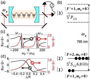
Figure 1: Conditional spin squeezing by homodyne probing of the collective population of atomic states. Panel (a) shows $N$ rubidium-87 atoms inside an optical cavity, and balanced homodyne detection of the field mixing the probe field of frequency $\omega_{p}$ and the field transmitted through the cavity. Panel (b) shows the energy diagram of the rubidium-87 atoms with two hyper-fine ground states, represented as the up and down state of a spin 1/2-particle, and an electronic excited state, coupling strongly with the optical cavity and leading to two atom-photon dressed states with transition frequencies $\omega_{\pm}$ (dashed lines). Panel (c) shows the intra-cavity field amplitude $\langle\hat{a}\rangle$ as function of $\omega_{p}$ (relative to the atomic transition frequency $\omega_{32}$) for the atomic ensemble prepared in an equal superposition of the two hyper-fine ground states. Panel (d) shows $\langle\hat{a}\rangle$ as a function of the imbalance of the two ground state populations $J_{z}/N$ for a fixed probe frequency $\omega_{p}=\omega_{32}+\sqrt{N/2}g$. For more details see text.

As a special case of the quantum theory of measurements, quantum systems subject to continuous measurements can be described by a stochastic master equation (SME)  (HMWiseman, ). So far, the SME has been restricted to small quantum systems, while for large systems, an approximate Gaussian-state formalism (BLMadsen, ) permits characterization of the system by mean values and covariances (first and second moments) of few collective observables. While the Gaussian state Ansatz may not generally apply, and in this Letter, we present an alternative and more general framework by deriving mean values of observables and their products from the SME, and truncating the resulting hierarchy of equations with a cumulant expansion approximation (DPlankensteiner, ). The obtained first and second moments of the observables are directly related to the mean and variance of the Gaussian-state formalism, and our derivation permits also the direct inclusion of spontaneous emission and dephasing of individual atoms. Furthermore, by assuming symmetry under exchange of the atoms, mean-field quantities are the same for all the atoms and for all atom pairs (DMeiser2009, ). Thus, irrespective of the number of atoms in the experimental system, we only need to consider tens of coupled stochastic non-linear differential equations in the simulations.

We study the conditional squeezing of $N$ rubidium-87 atoms in an optical cavity by homodyne detection with a probe laser of frequency $\omega_{p}$ [Fig. 1(a)], while the experiments in Ref. (ZChen, ; JGBohnet, ) applied heterodyne detection. We treat two hyper-fine ground states of rubidium-87 atoms, $\left|5^{2}\mathrm{S}_{1/2},F=1,m_{F}=0\right\rangle$ and $\left|5^{2}\mathrm{S}_{1/2},F=2,m_{F}=0\right\rangle$, as the spin up and down states of a spin $1/2$-particle, leading to the definition of collective spin operators $\hat{J}_{i}=\frac{1}{2}\sum_{k=1}^{N}\hat{\sigma}_{k}^{i}$ (with the Pauli matrices $\hat{\sigma}^{i}_{k}$ for $i=x,y,z$). An electronic excited state $\left|5^{2}\mathrm{P}_{1/2},F^{\prime}=1,m_{F}=0\right\rangle$ couples strongly with the upper hyper-fine ground state by resonant absorption of a cavity photon, leading to two atom-photon dressed states, split in energy by the collective coupling strength [Fig. 1(b)]. The collective operators constitute the collective mean spin vector ${\bf J}=\sum_{i=x,y,z}J_{i}{\bf e}_{i}$ with components $J_{i}=\langle\hat{J}_{i}\rangle$ (and the unit vectors ${\bf e}_{i}$ of the Cartesian coordinate system), and the uncertainty of these components $\Delta J_{i}=\sqrt{\langle\hat{J}_{i}^{2}\rangle-J_{i}^{2}}$ further characterize the states of the atomic ensemble.

In the homodyne detection of the transmitted probe signal, the photo-current is proportional to the real part of the intra-cavity field amplitude ${\rm Re}\langle\hat{a}\rangle$. This amplitude explores the resonances around the the dressed state energies, which are associated with the collective atom-cavity coupling strengths and hence with the population of the upper hyper-fine ground state, $J_{z}+N/2$. The homodyne signal thus measures the z-component of the collective spin vector $J_{z}$, and hence squeezes its uncertainty. To maximize the conditional spin squeezing, we examine first the variation of $\langle\hat{a}\rangle$ as function of the probe field frequency $\omega_{p}$ for the atomic ensemble on one spin coherent state with e.g. $J_{z}=J_{x}=0,J_{y}=N/2$, and we find that the real ${{\rm Re}\langle\hat{a}\rangle}$ and imaginary part ${{\rm Im}\langle\hat{a}\rangle}$ show narrow features around the frequencies of the dressed states $\omega_{\pm}=\omega_{32}\pm\sqrt{N/2}g$, respectively [Fig. 1(c)] (with $g$ as the coupling strength for single atom). We plot ${{\rm Re}\langle\hat{a}\rangle}$ and ${{\rm Im}\langle\hat{a}\rangle}$ as function of $J_{z}$ for $\omega_{p}=\omega_{32}+\sqrt{N/2}g$ in Fig. 1(d). Here, the variation is due to the modification of the dressed state resonance frequency, $\omega_{\pm}=\omega_{32}\pm\sqrt{J_{z}+N/2}g$. The slope of ${{\rm Re}\langle\hat{a}\rangle}$ and, hence, of the homodyne detection current to $J_{z}$ is largest, and the squeezing is optimal for variations of $J_{z}$ around $J_{z}=0$.

Stochastic Master Equation—

To describe the conditional dynamics of the atoms and cavity system as shown in Fig. 1, we develop the following stochastic master equation for the density operator $\hat{\rho}_{I}$ conditional on the photoncurrent $I$ of the homodyne detection:

$$\frac{\partial}{\partial t}\hat{\rho}_{I}=-\frac{i}{\hbar}\left[\hat{H}_{c}+\hat{H}_{p}+\hat{H}_{a}+\hat{H}_{a-c}+\hat{H}_{a-m},\hat{\rho}_{I}\right]$$

$$-\kappa\mathcal{D}\left[\hat{a}\right]\hat{\rho}_{I}-\gamma\sum_{k=1}^{N}\mathcal{D}\left[\hat{\sigma}_{k}^{23}\right]\hat{\rho}_{I}-(\chi/2)\sum_{k=1}^{N}\mathcal{D}\left[\hat{\sigma}_{k}^{22}-\hat{\sigma}_{k}^{33}\right]\hat{\rho}_{I}$$

$$+\frac{dW}{dt}\sqrt{\eta\kappa_{2}}\left[e^{i\omega_{p}t}\left(\hat{a}-\left\langle\hat{a}\right\rangle\right)\hat{\rho}_{I}+e^{-i\omega_{p}t}\hat{\rho}_{I}\left(\hat{a}^{\dagger}-\left\langle\hat{a}^{\dagger}\right\rangle\right)\right].$$ (1)

The first line of Eq. (1) describes the coherent dynamics. The optical cavity is described by the Hamiltonian $\hat{H}_{c}=\hbar\omega_{c}\hat{a}^{\dagger}\hat{a}$ with the frequency $\omega_{c}$, the photon creation $\hat{a}^{\dagger}$ and annihilation operator $\hat{a}$. The probing of the cavity by a laser beam of frequency $\omega_{p}$ is described by the Hamiltonian $\hat{H}_{p}=\hbar\Omega_{p}\sqrt{\kappa_{1}}\left(e^{i\omega_{p}t}\hat{a}+e^{-i\omega_{p}t}\hat{a}^{\dagger}\right)$ with the transmission coefficient $\sqrt{\kappa_{1}}$ of the left input mirror ($\kappa_{1}$ is the corresponding photon loss rate), and the probe amplitude parameterized by the strength $\Omega_{p}$. The ensemble of $N$ atoms is described by the Hamiltonian $\hat{H}_{a}=\hbar\sum_{k=1}^{N}\left(\omega_{1}\hat{\sigma}_{k}^{11}+\omega_{2}\hat{\sigma}_{k}^{22}+\omega_{3}\hat{\sigma}_{k}^{33}\right)$ with the frequencies $\omega_{l}$ and the projection operators $\hat{\sigma}_{k}^{ll}=\left|l_{k}\right\rangle\left\langle l_{k}\right|$ of the atomic states labeled by $l=1,2,3$ [Fig. 1(b)]. The atom-cavity interaction is described by the Hamiltonian $\hat{H}_{a-c}=\hbar g\sum_{k}\left(\hat{a}^{\dagger}\hat{\sigma}_{k}^{23}+\hat{\sigma}_{k}^{32}\hat{a}\right)$ with the coupling strength $g$, the lowering $\hat{\sigma}_{k}^{23}=\left|2_{k}\right\rangle\left\langle 3_{k}\right|$ and raising operator $\hat{\sigma}_{k}^{32}=\left|3_{k}\right\rangle\left\langle 2_{k}\right|$ between the excited state and the upper hyper-fine ground state. In addition, a classical microwave field with frequency $\omega_{m}$ drives the atomic ground hyper-fine transition as described by the Hamiltonian $\hat{H}_{d}=\hbar\Omega_{m}\left(e^{i\omega_{m}t}\sum_{k}\hat{\sigma}_{k}^{12}+e^{-i\omega_{m}t}\sum_{k}\hat{\sigma}_{k}^{21}\right)$ with strength $\Omega_{m}$. Here, $\omega_{l}$, $g$, $\Omega_{m}$ are assumed to be same for all the atoms.

The second line of Eq. (1) describes dissipation in the system with the Lindblad super-operator $\mathcal{D}\left[\hat{o}\right]\hat{\rho}=\frac{1}{2}\left(\hat{o}^{\dagger}\hat{o}\hat{\rho}+\hat{\rho}\hat{o}^{\dagger}\hat{o}-2\hat{o}\hat{\rho}\hat{o}^{\dagger}\right)$ (for any operator $\hat{o}$). The first term describes the cavity photon loss with a rate $\kappa=\kappa_{1}+\kappa_{2}$, where $\kappa_{2}$ is the photon loss rate through the right mirror. The second term describes the spontaneous emission of individual atoms from the excited state to the upper hyper-fine ground state with a rate $\gamma$, while the third term accounts for the dephasing of the atomic coherence between these states with a rate $\chi$. The last line of Eq. (1) describes the measurement back-action of the homodyne detection with the photon-shot noise, modeled by a Wiener increment $dW$ following a normal distribution with mean $E\left[dW\right]=0$ and variance $dW^{2}=dt$. The photocurrent difference between the two photodetectors (with an efficiency $\eta$) $I\left(t\right)=\sqrt{\eta\kappa_{2}}\mathrm{Re}\left\langle\hat{a}\right\rangle(t)+dW/dt$ is proportional to the real part of the intra-cavity field amplitude ${\rm Re}\left\langle\hat{a}\right\rangle$ but is domianted by the white noise $dW/dt$ at short time. Spontaneous decay of the individual atoms from the excited state to the lower hyper-fine ground state can be easily incorporated by extra Lindblad terms but is omitted here for simplicity.

In the mean-field theory, we derive equations $\partial_{t}\left\langle\hat{o}\right\rangle={\rm tr}\{(\partial_{t}\hat{\rho}_{I})\hat{o}\}$ for the mean value $\left\langle\hat{o}\right\rangle$ of the operator $\hat{o}$ from the SME (1). The cavity mean-field $\left\langle\hat{a}\right\rangle$, the atomic coherences $\left\langle\hat{\sigma}^{lm}_{k}\right\rangle$ (for $l,m=1,2,3$ and $l\neq m$) and the atomic level populations $\left\langle\hat{\sigma}^{ll}_{k}\right\rangle$, couple to second order moments, like the cavity photon number $\left\langle\hat{a}^{\dagger}\hat{a}\right\rangle$, atom-photon correlations $\left\langle\hat{a}^{\dagger}\hat{\sigma}_{k}^{23}\right\rangle$, and atom-atom correlations $\left\langle\hat{\sigma}_{k}^{lm}\hat{\sigma}_{k^{\prime}}^{l^{\prime}m^{\prime}}\right\rangle$ (for $k\neq k^{\prime}$). These quantities, in turn, couple to higher-order moments, leading to a hierarchy of equations. To terminate this hierarchy and obtain a closed set of coupled equations, we approximate higher-order mean-field terms e.g. $\left\langle\hat{o}\hat{p}\hat{q}\right\rangle$ with the products of lower-order mean-field terms e.g. $\left\langle\hat{o}\right\rangle\left\langle\hat{p}\hat{q}\right\rangle+\left\langle\hat{p}\right\rangle\left\langle\hat{o}\hat{q}\right\rangle+\left\langle\hat{q}\right\rangle\left\langle\hat{o}\hat{p}\right\rangle-2\left\langle\hat{o}\right\rangle\left\langle\hat{p}\right\rangle\left\langle\hat{q}\right\rangle$ (for any operators $\hat{o},\hat{p},\hat{q}$). Furthermore, by assuming the same parameters $g,\omega_{p},\Omega_{p},\omega_{m},\Omega_{m},\gamma,\chi$ for all atoms, we find that terms like $\left\langle\hat{\sigma}^{lm}_{k}\right\rangle$,$\left\langle\hat{\sigma}^{ll}_{k}\right\rangle$, $\left\langle\hat{a}^{\dagger}\hat{\sigma}_{k}^{23}\right\rangle$ are the same for all the atoms, and terms $\left\langle\hat{\sigma}_{k}^{lm}\hat{\sigma}_{k^{\prime}}^{l^{\prime}m^{\prime}}\right\rangle$ are same for all atom pairs $(k,k^{\prime})$. By exploring this property, we reduce the number of coupled nonlinear differential equations from the order of $\sim N^{3}$ to a few tens.

The symbolic QuantumCumulants.jl package (DPlankensteiner, ) can be applied to implement the cumulant expansion approximation and solve the deterministic master equation in the absence of measurements. We have modified this package and supplemented the code with a package StochasticDiffEq.jl to incorporate the stochastic measurement back action at the level of first and second order mean field quantities (YuHH, ). We show the codes and the equations derived to solve the SME in the Appendix  A and  C.

Spin squeezing can be quantified by the parameter (JMa, ) $\xi_{z}^{2}=N\left(\Delta J_{z}\right)^{2}/(J_{x}^{2}+J_{y}^{2})$. To calculate this parameter, we identify the Pauli operators $\hat{\sigma}^{x}_{k}=\left(\hat{\sigma}_{k}^{12}+\hat{\sigma}_{k}^{21}\right)$, $\hat{\sigma}^{y}_{k}=i\left(\hat{\sigma}_{k}^{12}-\hat{\sigma}_{k}^{21}\right)$ and $\hat{\sigma}^{z}_{k}=\left(2\hat{\sigma}_{k}^{22}-1\right)$. For the case of identical atoms, the components of the collective spin vector can be computed as $J_{x}=(N/2)\left(\left\langle\hat{\sigma}_{1}^{12}\right\rangle+\left\langle\hat{\sigma}_{1}^{21}\right\rangle\right)$, $J_{y}=(iN/2)\left(\left\langle\hat{\sigma}_{1}^{12}\right\rangle-\left\langle\hat{\sigma}_{1}^{21}\right\rangle\right)$, $J_{z}=(N/2)\left(2\left\langle\hat{\sigma}_{1}^{22}\right\rangle-1\right)$, and their uncertainties $\Delta J_{i}=\sqrt{\langle\hat{J}_{i}^{2}\rangle-J_{i}^{2}}$ can be computed with $\langle\hat{J}_{x/y}^{2}\rangle=\pm(N/4)[\left(N-1\right)(\left\langle\hat{\sigma}_{1}^{12}\hat{\sigma}_{2}^{12}\right\rangle\pm\left\langle\hat{\sigma}_{1}^{12}\hat{\sigma}_{2}^{21}\right\rangle\pm\left\langle\hat{\sigma}_{1}^{21}\hat{\sigma}_{2}^{12}\right\rangle+\left\langle\hat{\sigma}_{1}^{21}\hat{\sigma}_{2}^{21}\right\rangle)\pm 1]$, $\langle\hat{J}_{z}^{2}\rangle=(N/4)[4\left(N-1\right)(\left\langle\hat{\sigma}_{1}^{22}\hat{\sigma}_{2}^{22}\right\rangle-\left\langle\hat{\sigma}_{1}^{22}\right\rangle)+N]$. In the following simulations, we consider a system similar to the one studied in the experiments (ZChen, ), and we summarize the parameters in Tab. A1.

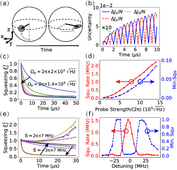
Figure 2: Conditional spin squeezing with different probe amplitudes $\Omega_{p}$ and frequency detunings $\delta=\omega_{p}-\omega_{+}$ (to upper dressed state). Panel (a) shows the collective spin vector ${\bf J}=J_{y}{\bf e}_{y}$ (black arrow) and its uncertainty (transparent circle) for the spin coherent state (left), and the rotated spin vector and squeezed uncertainty along the z-axis (transparent ellipse) for the spin squeezed state after probing (right). Panel (b) shows the uncertainties $\Delta J_{x},\Delta J_{y}$ (blue solid and red dashed line), and $\Delta J_{z}$ (green dotted line) for $\delta=0$ and $\Omega_{p}=2\pi\times 10^{4}\sqrt{\rm Hz}$. Panel (c) and (e) show the spin squeezing parameter $\xi_{z}^{2}$ as function of time for different $\Omega_{p}$ and fixed $\delta=\sqrt{N/2}g$, and for different $\delta$ and fixed $\Omega_{p}=2\pi\times 10^{4}\sqrt{\rm Hz}$, respectively, where the dashed curves are fitted with function specified in the main text. Panel (d) and (f) summarize the squeezing rate and the minimal value of $\xi_{z}^{2}$. Here, we consider an ideal system with $N=10^{4}$ atoms in the absence of individual atomic dissipations.

Conditional Spin Squeezing–

In Fig. 2, we show the behavior of spin mean values and variances during the homodyne detection. In our simulation, we first prepare the atomic ensemble in a spin coherent state such that the collective spin vector points along the y-axis and has equal uncertainty along the x- and z-axis [left of Fig. 2(a)]. Our calculations show that during the laser probing the collective spin vector components $J_{x}$ and $J_{y}$ oscillate with time, while the component $J_{z}$ is slightly reduced [Fig. A3]. At the same time, the uncertainty $\Delta J_{z}$ decreases due to the measurement backaction while $\Delta J_{x},\Delta J_{y}$ oscillate in time with increasing amplitude [Fig. 2(b)]. These results indicate that the collective spin vector rotates around the z-axis, and the spin squeezing and anti-squeezing occur for the collective spin component along the z-axis and in the equatorial plane, respectively [right of Fig. 2(a)]. Note that the uncertainty $\Delta J_{\parallel}=\sqrt{\Delta J_{x}^{2}+\Delta J_{y}^{2}}$ follows the oscillation envelope in Fig. 2(b), and the rotation in the equatorial plane can be explained by the probe field-dependent AC Stack shift of the upper hyper-fine ground state of the atoms (Fig. A3).

Accompanying the above dynamics, the spin squeezing parameter $\xi_{z}^{2}$ decreases rapidly in the beginning, and then it slowly saturates to a finite value or increases for longer time [Fig. 2(c) and (e)]. Earlier studies (BLMadsen, ) motivate the fitting of this dynamics with a function $\xi_{z}^{2}(t)=A/(1+k_{1}t)+(1-A)e^{k_{2}t}$, and we extract the pertaining squeezing rate $k$, the anti-squeezing $k_{2}$ and the minimal squeezing value. As the probe strength increases, the spin squeezing occurs faster and its minimal value increases [Fig. 2 (c,d)], which agree qualitatively with the experimental results (JGBohnet, ). When the frequency detuning $\delta=\omega_{p}-\omega_{+}$ of the probe field $\omega_{p}$ to the upper dressed state increases, the spin squeezing is slower for short time, reaches a minimum and rises to values above unity for longer time [Fig. 2(e)]. As a result, the squeezing rate $k_{1}$ and the minimal squeezing are maximized and minimized for a vanishing probe frequency detuning [Fig. 2(f)]. At the same time, the rate of anti-squeezing $k_{2}$ is minimized for the near-resonant condition $\delta\approx 0$ (not shown). Furthermore, we find that the spin squeezing is stronger for larger detection efficiency, and optimal under the atom-cavity resonance conditions (Fig. A4).

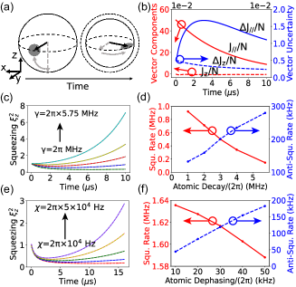
Figure 3: Influence of individual atomic dissipation on the conditional spin squeezing. Panel (a) shows that the change of the collective spin vector and its uncertainty in the presence of individual atomic decay process. Panel (b) shows the length of the vector projection $J_{\parallel}\equiv\sqrt{J_{x}^{2}+J_{y}^{2}}$ and the vector z-component $J_{z}$ (left axis), and their uncertainties $\Delta J_{\parallel}\equiv\sqrt{\Delta J_{x}^{2}+\Delta J_{y}^{2}}$, $\Delta J_{z}$ (right axis). Panel (c) and (e) show the spin squeezing parameter $\xi_{z}^{2}$ for increasing atomic decay rate $\gamma$ and dephasing rate $\chi$, respectively. In these panels, the solid curves are fitted with functions given in the main text, and the extracted squeezing and anti-squeezing rates are shown in panels (d) and (f), respectively. Other parameters are the same as in Fig. 2.

Influence of the Individual Atomic Dissipation on Conditional Spin Squeezing —

In Fig. 3, we investigate how the decay and dephasing of individual atoms affect the conditional spin squeezing. As shown pictorially in Fig. 3(a), these processes affect the degree of spin squeezing mainly by reducing the length of the collective spin vector. More precisely, in the presence of individual decay, the collective spin vector projection in the equatorial plane $J_{\parallel}=\sqrt{J_{x}^{2}+J_{y}^{2}}$ decreases with time, while its uncertainty $\Delta J_{\parallel}=\sqrt{(\Delta J_{x})^{2}+(\Delta J_{y})^{2}}$ first increases and then decreases [Fig. 3(b)]. In addition, the collective spin vector component $J_{z}$ and its uncertainty $\Delta J_{z}$ are less than in the ideal case. As a result, after an initial decrease, the spin squeezing parameter $\xi_{z}^{2}$ increases dramatically [Fig. 3(c)]. More precisely, as the atomic decay rate $\gamma$ increases to $2\pi\times 5.75$ MHz (the typical value for rubidium atoms), $\xi_{z}^{2}$ decreases only slowly for short times, and increases more dramatically for longer times, cf. the fitted values of the squeezing and anti-squeezing rate $k_{1}$ and $k_{2}$ [Fig. 3(d)]. Note that for the higher decay rate, the minimal $\xi_{z}^{2}$ becomes larger and occurs at earlier times [Fig. A5(a)].

The atomic dephasing rate $\chi$ affects the collective spin vector and the conditional spin squeezing [Fig. 3(e,f) and Fig. A5(b)] in a similar way as the atomic decay rate, except that the collective spin vector component $J_{z}$ also decreases with time (not shown). For similar values of the atomic decay and dephasing rates, we find that atomic dephasing affects the spin squeezing more strongly.

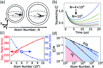
Figure 4: Dependence of conditional spin squeezing on the number of atoms $N$ and the Heisenberg limit. Panel (a) shows that the length reduction of the collective spin vector due to the individual atomic decay and dephasing (with rates $\gamma,\chi$) can be compensated by increasing $N$. Panel (b) shows the spin squeezing parameter $\xi_{z}^{2}$ as function of $N$ for $\gamma=2\pi\times 5.75$ MHz and $\chi=2\pi\times 10$ kHz, and panel (c) shows the extracted spin squeezing and anti-spin squeezing rates. Panel (d) shows the ratio $\xi_{z}^{2}/N$ as function of $N$ for spin coherent states (black dots and line), which can be fitted by $\xi_{z}^{2}/N\sim 1/N$ (i.e. standard quantum limit, SQL), and for spin squeezed states in the absence (red dots and line) and presence (blue dots and line) of the individual atomic decay rate, where they can be fitted with $\xi_{z}^{2}/N\sim 1/N^{2}$ (i.e. Heisenberg limit, HL) and $\xi_{z}^{2}/N\sim 1/N^{8/5}$ (between SQL and HL), respectively.

Spin Squeezing as Function of the Number of Atoms and the Heisenberg Limit —

The detrimental affects of the individual atomic dissipation can be mitigated simply by increasing the number of atoms $N$, as illustrated in Fig. 4(a-c). As $N$ increases from $4\times 10^{4}$ to $10^{5}$, the initial decrease of the spin squeezing parameter $\xi_{z}^{2}$ becomes faster, and its later raising becomes slower, i.e. the approach to the ideal systems. More precisely, the spin squeezing rate $k_{1}$ increases from $317$ kHz to $375$ kHz, while the anti-squeezing rate $k_{2}$ decreases from $86$ kHz to $50$ kHz. At the same time, the minimal squeezing also decreases and occurs later [Fig. A5(c)].

By obtaining the minimal spin squeezing for different $N$, we can calculate the ratio $\xi_{z}^{2}/N$ as function of $N$ [Fig. 4(d)]. Note that in the literature (ZChen, ; JGBohnet, ), the polar angle $\theta_{B}=J_{z}/J_{\parallel}$ is often introduced to characterize the states of the atomic ensemble, and its variance equal to the ratio $\xi_{z}^{2}/N$ is usually used to witness the spin squeezing. For the system in a spin coherent state, the results can be well fitted with the expression $\sim 1/N$ (black dots and line), indicating the so-called standard quantum limit (SQL). In contrast, for the ideal system without individual atomic decay, the results depart from the SQL line for $N$ larger than $10^{3}$, and can be well fitted with the formula $\sim 1/N^{2}$ (red dots and line), hinting at the so-called Heisenberg limit (HL). For the realistic system with atomic decay, the results deviate from the SQL line for $N$ larger than $10^{4}$, and they can be fitted with $\sim 1/N^{8/5}$ (blue dots and line), indicating a scaling between the SQL and HL. Note that the blue dots agree well with the experimental results (cf. Fig. 4 of Ref.  (JGBohnet, )). Beyond the simple squeezing parameters, our theory can be also applied to simulate how the conditional spin squeezing can be prepared and measured, providing further insights into possible experiments (see Fig. A6).

Conclusions —

In summary, we have developed a stochastic mean-field theory to solve the stochastic master equation (SME) with a cumulant-expansion mean-field approach. We have applied this method to conditional spin squeezing by continuous optical probing of the atomic hyper-fine state populations, enabled by their collective coupling to a cavity field and the homodyne detection of the transmitted field. In comparison to the full density matrix, our theory deals with only few mean-field quantities, and it can thus be applied to large quantum systems. In this article, we restricted the cumulant expansion to first and second order operator moments, and bridged the well-established collective Gaussian state formalism with the full SME theory. In particular, by dealing with mean values of individual atom and atom pair observables, our theory allows us to incorporate naturally the decay and the dephasing of individual atoms.

For the conditional spin squeezing of tens of thousands of rubidium 87 atoms coupled strongly with an optical cavity, our simulations showed clearly how the degree of spin squeezing is affected by the probe field (frequency and strength) and other parameters, how the decay and dephasing of individual atoms prevent the system from achieving the Heisenberg limit of sensitivity, and how these deleterious effects can be mitigated by increasing the number of atoms.

In the end, we emphasize that our theory can be extended straightforwardly to study conditional spin squeezing with heterodyne detection (ZChen, ), and deterministic spin squeezing with quantum feedback (LKThomsen, ; LKThomsenPRA, ; KCCox, ), and the squeezing transfer from nuclear transition (BBraverman, ) to optical clock transition (PPE, ). Also retrodictive spin squeezing beyond the Heisenberg uncertainty relation may be dealt with by a cumulant expansion version of the past quantum state formalism (HBao, ; HBaoNC, ).

Author Contributions

ZhiQing Zhang carried out the numerical calculations under the supervision of Yuan Zhang who developed the theory and the numerical programs. They contribute equally to the work. All authors contributed to the analysis of the results and the writing of the manuscript.

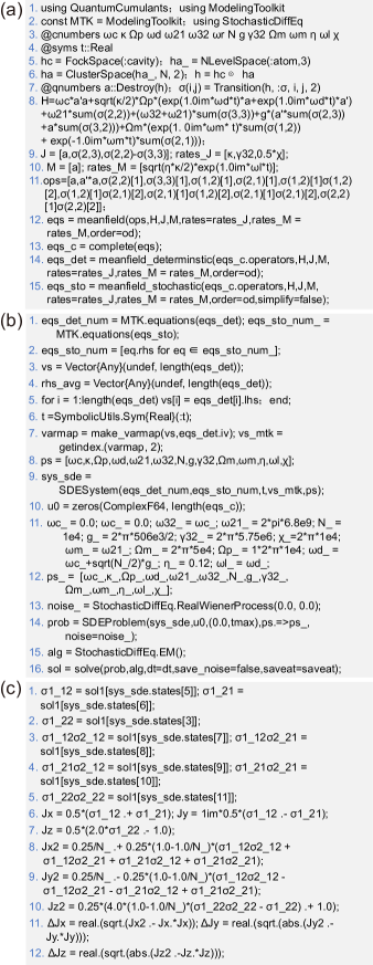
Figure A1: Julia codes to derive (a), solve (b) the stoachastic mean-field equations, and to extract the numerical results (c).

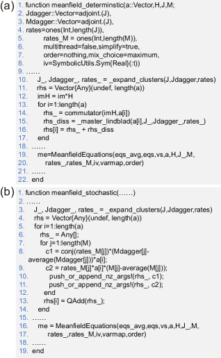
Figure A2: Partial code of the " meanfield_deterministic" function (a) and the " meanfield_stochastic" function (b).

Appendix A Julia Codes to Derive and Solve Stochastic Mean Field Equations

In this appendix, we present in Fig. A1 the Julia codes to derive (a) and solve (b,c) the stochastic mean-field equations.

In Fig. A1(a), lines 1,2 import the packages. Lines 3,4 define complex quantities and time argument as real number. Line 5 defines the Hilbert space of the optical cavity, and a three-level atom. Line 6 defines the special Hilbert space for the atomic ensemble, and the product Hilbert space for the atoms-cavity system. Line 7 defines the photon annihilation operator and the atomic transition operators. Line 8 defines the system Hamiltonian. Lines 9 and 10 define the list of operators and rates for the Lindblad terms and the measurement backaction, respectively. Line 11 defines the list of operators, line 12 derives the equations for the mean-value of these operators, line 13 derives the complete set of mean-field equations. Lines 14 and 15 define the equations for the deterministic and stochastic dynamics.

In Fig. A1(b), lines 1 and 2 define the numerical version of the equations for the deterministic and stochastic dynamics. Lines 3-7 define the list of variables. Line 8 defines the list of complex numbers. Line 9 defines the stochastic differential equation (SDE) system. Line 10 defines the initial values for the mean fields. Lines 11 and 12 specify the values for the complex numbers, and the list of these values. Line 13 defines the Wiener noise for the stochastic dynamics. Line 14 defines the SDE problem with given initial values, time range, parameters, and noise type. Line 15 specifies the Euler-Maruyama solver, and the list of simulation times. Line 16 solves the SDE problem.

In Fig. A1(c), lines 1,2 extract the coherence of the transition between the upper hyper-fine ground state and the excited state, and the population of the upper hyper-fine ground state. Lines 3-5 extract the atom-atom correlations. Lines 6,7 calculate the expectation values of the collective spin operators. Lines 8-10 calculate the expectation values of the squared collective spin operators. Lines 11,12 calculate the uncertainty of the collective spin vector components. The derived equation is shown in Appendix C.

While the QuantumCumulants.jl package is designed to solve the standard and deterministic quantum master equation, we have modified it to solve the stochastic master equation. In the modification, the most significant change is to define a new function "meanfield_stochastic" to derive the dependence of the mean-field quantities due to the measurement backaction.

In Fig. A2(a), we show the partial code for the "meanfield_deterministic" as a reference, which resembles the "meanfield" function in the QuantumCumulants.jl package. Line 1 defines the function with the necessary parameters. The first two parameters are the list of operators "a" to define the mean field quantities and the system Hamiltonian "H". The next two parameters are the list of operators "J,M" to define the Lindblad and stochastic term. Lines 2,3 define the conjugation "Jdagger,Mdagger" of "J,M". Lines 4,5 are the rates "rates,rates_M" associated to the Lindblad and stochastic term. Lines 6-8 define the remaining parameters. Among them, "order,iv" are the order of the mean-field approach, and the symbol for the time parameter. Line 10 translates the parameters "J,Jdagger" in Hilbert space to deal with the system within the identical particle assumption. Line 11 defines the array of operators with the same length as the list "a". Line 12 defines "imH" as the multiplication of the imaginary sign with the system Hamiltonian for convenience. Lines 13-17 computes the dependence due to the communication relation of "a" and "imH", and due to the Lindblad term, and forms the equations for the operators in the list "a". We transfer these equations into "eqs_avg" for the mean-field quantities by using the "average()" function (not shown). Lines 19-20 define the object "me" to represent the derived mean-field equations. One should note that in this function the lists "M,Mdagger,M_rates" for the stochastic terms are used only for the definition of the object "me".

In Fig. A2(b), we show the partial code for the "meanfield_stochastic" function. In comparison to the "meanfield_deterministic" function, only the code lines 5-14 are different. Here, we define first an empty list "rhs_", and we then enumerate every term in the list "M", and compute the dependence "c1,c2" due to the corresponding stochastic terms, and push them into the list "rhs_", and finally add the terms in the list to form the equations for the operator in the list "a". Here, the most important step is to introduce the mean-field terms through the "average()" functions into the equations for the operators. In lines 16-20, we define again the object "me" to represent the derived mean-field equations. One should note that in this function the lists "J,Jdagger,J_rates" for the stochastic terms are used only for the definition of the object "me".

In our code a single cavity mode is treated as a component of the system. Often, one may eliminate the cavity mode and deal only with a stochastic master equation for the atoms, where the cavity coupling enters through collective energy shifts and decay rates. We have verified that the above modified code can be also applied to solve this simplified equation.

Appendix B Supplemental Results

In this appendix, we provide extra results to complement the discussions in the main text.

$\omega_{c}$	$2\pi\times 377$ THz	$\omega_{21}$	$2\pi\times 6.8$ GHz
$\kappa$	$2\pi\times 11.1$ MHz	$\omega_{m}$	$\omega_{21}$
$\omega_{32}$	$\omega_{c}$	$\Omega_{m}$	$2\pi\times 10^{6}$ $\rm\sqrt{Hz}$
$g$	$2\pi\times 0.253$ MHz	$\omega_{p}$	$\omega_{c}+\sqrt{N/2}g$
$\gamma$	$2\pi\times 5.75$ MHz	$\Omega_{p}$	$2\pi\times 10^{4}$ $\rm\sqrt{Hz}$
$N$	$10^{4}$	$\eta$	$0.12$
$\chi$	$2\pi\times 10$ kHz

Table A1: System parameters for the simulations in the main text and this supplemental material.

B.1 System Parameters

Here, we summarize the parameters used in our simulations, see also Tab. A1. The optical cavity mode has a frequency $\omega_{c}=2\pi\times 377$ THz, and a photon damping rate $\kappa=2\pi\times 11.1$ MHz. The atomic transition between the upper hyper-fine ground state and the excited state has a frequency $\omega_{32}=\omega_{c}$, and couples to the cavity mode with a strength $g=2\pi\times 0.253$ MHz, has a decay rate $\gamma=2\pi\times 5.75$ MHz and a dephasing rate $\chi=2\pi\times 10$ kMz. The atomic transition between the two hyper-fine ground states has a frequency $\omega_{21}=2\pi\times 6.8$ GHz, and couples resonantly with the microwave drive field, i.e. $\omega_{m}=\omega_{21}$, with a strength $\Omega_{m}=2\pi\times 10^{6}$ $\rm\sqrt{\rm Hz}$. In addition, the optical cavity is probed by a laser with a frequency $\omega_{p}=\omega_{c}+\sqrt{N/2}g$ and a strength $\Omega_{p}=2\pi\times 10^{4}$ $\rm\sqrt{Hz}$, and the photo-detector of the homodyne detection has a detection efficiency $\eta=0.12$.

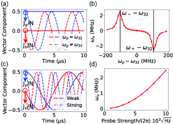
Figure A3: Collective spin vector rotation due to ac Stark effect. Panel (a) shows the dynamics of the collective spin vector components $J_{x}$ (red lines) and $J_{y}$ (blue lines), which are normalized to the number of atoms $N$, for the probe field with frequency detuned ($\omega_{p}=\omega_{32}+2\pi\times 20$ MHz, dashed lines) and resonant ($\omega_{p}=\omega_{32}$, solid lines) to the atomic transition between the upper hyper-fine ground state and the excited state, and given field strength $2\pi\times 10^{4}\sqrt{\rm Hz}$. Panel (b) shows the frequency $\omega_{o}$ of $J_{x}$ and $J_{y}$ oscillations as function of the probe field frequency (relative to the the atomic transition frequency $\omega_{32}$) for given probe field strength, which shows resonances at the frequencies $\omega_{\pm}$ of the atom-photon dressed states. Panel (c) shows the dynamics of $J_{x}$ and $J_{y}$ for the probe field with a strong strength $2\pi\times 10^{4}\sqrt{\rm Hz}$ (dashed lines) and a relatively weak one $2\pi\times 0.5\times 10^{4}\sqrt{\rm Hz}$ (solid lines), which is resonant to the atom-photon dressed state with larger frequency, i.e. $\omega_{p}=\omega_{+}$. Panel (d) shows the frequency $\omega_{o}$ of $J_{x}$ and $J_{y}$ oscillations as function of the probe field strength, which can be well fitted with a quadratic function. In all the simulations, the atomic transition is assumed to be resonant with the cavity mode, i.e. $\omega_{32}=\omega_{c}$. Other parameters are same as those in Fig. 2 of the main text.

B.2 Collective Spin Vector Rotation due to AC Stark-Shift

In the main text, we show that the collective spin vector rotates in the equatorial plane during the laser probing of the atomic ensemble. We show in Fig. A3 that this rotation depends on the frequency and strength of the probe field. The rotation occurs only for a probe field detuned from the atomic transition between the upper hyper-fine ground state and the excited state [Fig. A3(a)], and the frequency of oscillations shows two maxima when the probe frequency is resonant with the two atom-photon dressed states [Fig. A3(b)]. In addition, the oscillations become faster when the probe field strength is increased [Fig. A3(c)], and the oscillation frequency scales quadratically with the probe field strength. The oscillations are readily explained by the ac Stark frequency shift of the ground state of the coupled atoms-cavity system by $\delta_{ac}=-\Omega_{p}^{2}/\Delta_{1}-\Omega_{p}^{2}/\Delta_{2}$, where $\Delta_{1},\Delta_{2}$ are the frequency detunning of the probe field and the lower and upper dressed state, respectively.

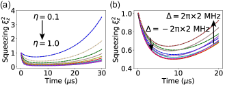
Figure A4: Influence of detection efficiency $\eta$ of photo-detectors (a) and the atom-cavity frequency detuning $\Delta=\omega_{32}-\omega_{c}$ (b) on the dynamics of conditional spin squeezing. In these simulations, we consider the fixed probe strength $\Omega_{p}=2\pi\times 10^{4}\rm\sqrt{Hz}$ and the presence of the atomic decay with rate $\gamma=2\pi\times 5.75$ $\rm MHz$. Other parameters are same as those in Fig. 2 of the main text.

B.3 Influence of Detection Efficiency on Conditional Spin Squeezing 

In the simulations in the main text, we have assumed a realistic detector efficiency $\eta=0.12$ and a resonant condition $\Delta=\omega_{32}-\omega_{c}=0$ between the upper hyper-fine ground-excited state transition and the cavity mode. In Fig. A4, we investigate how the efficiency $\eta$ (a) and the frequency detuning $\Delta$ (b) affect the conditional spin squeezing. As $\eta$ increases from $0.1$ to $1.0$, the reduction of the initial squeezing parameter becomes much faster, and its minimum becomes gradually lower, while its final increase become more slow. As $\Delta$ increases from negative to positive value within several megahertz, the initial fall of squeezing parameter becomes firstly faster and then slower, and the latter raising behaves similarly.

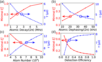
Figure A5: Influence of different parameters on minimal squeezing parameter $\xi_{z}^{2}(\tau)$ (left axes) and the corresponding time $\tau$ (right axes). Panel (a) and (b) show the results for increasing atomic decay rate $\gamma$, and atomic dephasing rate $\chi$, respectively. Panel (c) and (d) show the results for increasing atom number $N$, and increasing detection efficiency $\eta$, respectively. Other parameters are same as Tab. A1.

B.4 Influence of Different Parameters on Minimal Spin Squeezing and the Corresponding Time

In the main text, we study the influence of the atomic decay, the atomic dephasing and the number of atoms on spin squeezing, and discussed the effect of the detection efficiency of the photondetector in Appendix B.3. In the presence of the individual atomic dissipation, the spin squeezing parameter first decreases and then increases, and can be fitted with the function $\xi^{2}_{z}(t)=A/(k_{1}t+1)+(1-A)e^{k_{2}t}$. Except for the the squeezing and anti-squeezing rate $k_{1}$, $k_{2}$, we can also extract the minimal squeezing parameter $\xi^{2}_{z}(\tau)$ and the corresponding time $\tau=2W(s)/k_{2}-1/k_{1}$ (with the abbreviation $s\equiv[k_{2}/(2k_{1})]\sqrt{\frac{A}{1-A}\frac{k_{1}}{k_{2}}e^{\frac{k_{2}}{k_{1}}}}$). Here, $W(s)$ is a Lambert W function.

Here, we study the influence of different parameters on $\xi^{2}_{z}(\tau)$ and $\tau$[Fig. A5]. As the individual atomic decay rate $\gamma$ increases within few MHz, $\xi^{2}_{z}(\tau)$ increases from about $0.3$ to $1.0$, and $\tau$ decreases from $6$ $\mu$s to almost zero [Fig. A5(a)]. As the individual atomic dephasing rate $\chi$ increases within tens of MHz, $\xi^{2}_{z}(\tau)$ increases from about $0.2$ to $0.4$, and $\tau$ decreases from $10$ $\mu$s to $3$ $\mu$s [Fig. A5(b)]. Thus, the atomic dephasing deteriorates the spin squeezing more strongly than dephasing, see also Fig. 3 of the main text.

In contrast, as the number of atoms $N$ increases from $4\times 10^{4}$ to $10^{5}$, $\xi^{2}_{z}(\tau)$ decreases from about $0.6$ to about $0.35$, and $\tau$ increases from $6$ $\mu$s to $12$ $\mu$s [Fig. A5(c)]. As the detection efficiency $\eta$ increases from $0.12$ to unity, $\xi^{2}_{z}(\tau)$ decreases exponentially from about $0.8$ to $0.1$, and $\tau$ increases from $6$ $\mu$s to the saturated value $8$ $\mu$s [Fig. A5(d)].

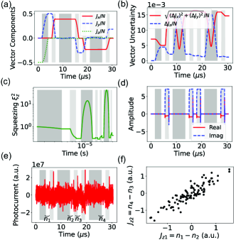
Figure A6: Simulation of generation and verification of the conditional spin squeezing. Panel (a) shows the dynamics of the collective spin vector components $J_{x}/N,J_{y}/N,J_{z}/N$ (red solid, blue dashed, green dotted line) during the application of three microwave field pulses (gray areas) and four laser probe pulses (light areas). Panel (b) shows the uncertainty of the vector projection in the equator plane $\sqrt{(\Delta J_{x})^{2}+(\Delta J_{y})^{2}}/N$ (red solid line) and the vector component along the z-axis $\Delta J_{z}/N$ (blue dashed line), while panel (c) shows the spin squeezing parameter $\xi_{z}^{2}$. Panel (d) shows the real and imaginary part (blue solid and red dashed line) of the intra-cavity field amplitude. Panel (e) shows the dynamic of the photo-current in the homodyne detection, where the current during the four laser pulses are integrated to form the quantities $n_{i}$ ($i=1,2,3,4$). Panel (f) shows $J_{z,2}=n_{4}-n_{3}$ versus $J_{z,1}=n_{1}-n_{2}$ during the preparation and verification of the conditional spin squeezing for one hundred simulations. Other parameters are the same as in Fig. 2 of the main text.

B.5 Simulations of Generation and Verification of Conditional Spin Squeezing

In the main text, we have studied the influence of various processes on the conditional spin squeezing. In the following, we simulate the possible measurements to verify the conditional spin squeezing. Following the procedures as indicated in Fig. A6, which are similar to those in the experiment (ZChen, ), we apply first a microwave $\pi/2$-pulse to prepare the atomic ensemble in the spin coherent state, and then we apply two laser probe pulses intersected by a microwave $\pi$-pulse, and finally we repeat the procedures in the second step. The homodyne signals accumulated during the four laser pulses are proportional to the number of atoms in the upper hyper-fine ground state, and will be denoted as $n_{i}$ for $i=1,2,3,4$ in the following. The homodyne detection of the first two laser probe pulses generates the spin squeezing state, and the difference $J_{z,1}=n_{1}-n_{2}$ can be viewed as an estimation of the collective spin vector component $J_{z}$ along the z-axis during the whole preparation period. The second two probe pulses serve to verify the degree of the spin squeezing, and the difference $J_{z,2}=n_{4}-n_{3}$ estimate $J_{z}$ during the whole verification period. The conditional spin squeezing will be translated as the correlation between $J_{z,1}$ and $J_{z,2}$. If there was no spin squeezing, no correlation between $J_{z,1}$ and $J_{z,2}$ will be expected.

In Fig. A6, we demonstrate the system dynamics during the whole procedure as mentioned above. Fig. A6(a) and (b) show the dynamics of the collective spin vector components and their uncertainty. We see that after the first microwave pulse, the collective spin vector rotates around the x-axis and becomes parallel with the y-axis, and acquires equal uncertainty along the z-axis and the equatorial plane. During the remaining two microwave pulses, the collective spin vector is rotated by $180$ degree while its uncertainty is identical before and after the pulses. During the laser pulses, the collective spin vector rotates in the equatorial plane, the uncertainty reduces for the vector projection along the z-axis, but increases for the vector projection in the equatorial plane. Note that the vector projection along the z-axis reduces also slightly during the application of the laser pulses. Figure A6(c) shows that the spin squeezing parameter reduces during the application of laser pulses due to the QND measurement, but shows a pulse during the microwave pulses due to the rotation of the collective spin vector.

Figure A6(d) shows that the intra-cavity field has only values during the laser pulses, and the imaginary part is much larger than the real part. Figure A6(e) shows that the photon-current in the homodyne detection is dominated by the white noise, but is shifted downwards perceivablely during the application of the laser pulses. Figure A6(f) shows that $J_{z,1}$ and $J_{z,2}$ are correlated with each other, which verifies the conditional spin squeezing, which agree qualitatively with the experiment with heterodyne detection LABEL:ZChen. Since the spin squeezing parameter actually decreases in every laser pulse, the results in Fig. A6(c) should be considered in the sense of average for given period.

Appendix C Conditional Mean-field Equations

In this appendix, we present the mean-field equations derived from the conditional master equation (1) in the main text. In the current work, we apply the third order cumulants to approximate the mean fields $\left\langle\hat{o}\hat{p}\hat{q}\right\rangle$ with $\left\langle\hat{o}\right\rangle\left\langle\hat{p}\hat{q}\right\rangle+\left\langle\hat{p}\right\rangle\left\langle\hat{o}\hat{q}\right\rangle+\left\langle\hat{q}\right\rangle\left\langle\hat{o}\hat{p}\right\rangle-2\left\langle\hat{o}\right\rangle\left\langle\hat{p}\right\rangle\left\langle\hat{q}\right\rangle$ for any operators $\hat{o},\hat{p},\hat{q}$. In the following, we present firstly the equations for the first-order mean quantities. The cavity field amplitude $\langle\hat{a}\rangle$ satisfies the equation

$$\partial_{t}\langle\hat{a}\rangle=-i\left(\omega_{c}-i\kappa/2\right)\langle\hat{a}\rangle+iNg\langle\hat{\sigma}_{1}^{23}\rangle$$

$$-i\Omega_{p}\sqrt{\kappa/2}e^{-i\omega_{p}t}+\frac{dW}{dt}\sqrt{\eta\kappa/2}e^{i\omega_{p}t}\left(\langle\hat{a}\hat{a}\rangle-\langle\hat{a}\rangle^{2}\right)$$

$$+\frac{dW}{dt}\sqrt{\eta\kappa/2}e^{-i\omega_{p}t}\left(\langle\hat{a}^{\dagger}\hat{a}\rangle-\langle\hat{a}^{\dagger}\rangle\langle\hat{a}\rangle\right).$$ (2)

The atomic coherence $\left\langle\hat{\sigma}_{1}^{12}\right\rangle$, $\left\langle\hat{\sigma}_{1}^{13}\right\rangle$ and $\left\langle\hat{\sigma}_{1}^{23}\right\rangle$ follow the equations

$$\partial_{t}\langle\hat{\sigma}_{1}^{12}\rangle=(-i\omega_{21}-\chi/4)\langle\hat{\sigma}_{1}^{12}\rangle-ig\langle\hat{a}^{\dagger}\hat{\sigma}_{1}^{13}\rangle\rangle$$

$$+i\Omega_{m}e^{-i\omega_{m}t}\left(-1+\langle\hat{\sigma}_{1}^{33}\rangle+2\langle\hat{\sigma}_{1}^{22}\rangle\right)$$

$$+\frac{dW}{dt}\sqrt{\eta\kappa/2}e^{i\omega_{p}t}\left(\langle\hat{a}\hat{\sigma}_{1}^{12}\rangle-\langle\hat{a}\rangle\langle\hat{\sigma}_{1}^{12}\rangle\right)$$

$$+\frac{dW}{dt}\sqrt{\eta\kappa/2}e^{-i\omega_{p}t}\left(\langle\hat{a}^{\dagger}\hat{\sigma}_{1}^{12}\rangle-\langle\hat{a}^{\dagger}\rangle\langle\hat{\sigma}_{1}^{12}\rangle\right),$$ (3)

$$\partial_{t}\langle\hat{\sigma}_{1}^{13}\rangle=\left(-i\omega_{21}-i\omega_{32}-\gamma/2-\chi/4\right)\langle\hat{\sigma}_{1}^{13}\rangle$$

$$-ig\langle\hat{a}\hat{\sigma}_{1}^{12}\rangle+i\Omega_{m}e^{-i\omega_{m}t}\langle\hat{\sigma}_{1}^{23}\rangle$$

$$+\frac{dW}{dt}\sqrt{\eta\kappa/2}e^{i\omega_{p}t}\left(\langle\hat{a}\hat{\sigma}_{1}^{13}\rangle-\langle\hat{a}\rangle\langle\hat{\sigma}_{1}^{13}\rangle\right)$$

$$+\frac{dW}{dt}\sqrt{\eta\kappa/2}e^{-i\omega_{p}t}\left(\langle\hat{a}^{\dagger}\hat{\sigma}_{1}^{13}\rangle-\langle\hat{a}^{\dagger}\rangle\langle\hat{\sigma}_{1}^{13}\rangle\right),$$ (4)

$$\partial_{t}\langle\hat{\sigma}_{1}^{23}\rangle=\left(-i\omega_{32}-\gamma/2-\chi\right)\langle\hat{\sigma}_{1}^{23}\rangle$$

$$+ig\left(\langle\hat{a}\hat{\sigma}_{1}^{33}\rangle-\langle\hat{a}\hat{\sigma}_{1}^{22}\rangle\right)+i\Omega_{m}e^{i\omega_{m}t}\langle\hat{\sigma}_{1}^{13}\rangle$$

$$+\frac{dW}{dt}\sqrt{\eta\kappa/2}e^{i\omega_{p}t}\left(\langle\hat{a}\hat{\sigma}_{1}^{22}\rangle-\langle\hat{a}\rangle\langle\hat{\sigma}_{1}^{22}\rangle\right)$$

$$+\frac{dW}{dt}\sqrt{\eta\kappa/2}e^{-i\omega_{p}t}\left(\langle\hat{a}^{\dagger}\hat{\sigma}_{1}^{23}\rangle-\langle\hat{a}^{\dagger}\rangle\langle\hat{\sigma}_{1}^{23}\rangle\right).$$ (5)

Here and in the following, we do not consider the quantities like $\left\langle\hat{a}^{\dagger}\right\rangle,\left\langle\hat{\sigma}_{1}^{21}\right\rangle$ because they are the complex conjugation of other terms like $\left\langle\hat{a}\right\rangle,\left\langle\hat{\sigma}_{1}^{12}\right\rangle$. The equations for the populations of the upper hyper-fine ground state and the excited state $\left\langle\hat{\sigma}_{1}^{22}\right\rangle$, $\left\langle\hat{\sigma}_{1}^{33}\right\rangle$ take the form

$$\partial_{t}\langle\hat{\sigma}_{1}^{22}\rangle=\gamma\langle\hat{\sigma}_{1}^{33}\rangle-ig\left(\langle\hat{a}^{\dagger}\hat{\sigma}_{1}^{23}\rangle-\langle\hat{a}\hat{\sigma}_{1}^{32}\rangle\right)$$

$$+i\Omega_{m}(e^{i\omega_{m}t}\langle\hat{\sigma}_{1}^{12}\rangle-e^{-i\omega_{m}t}\langle\hat{\sigma}_{1}^{21}\rangle)$$

$$+\frac{dW}{dt}\sqrt{\eta\kappa/2}e^{i\omega_{p}t}\left(\langle\hat{a}\hat{\sigma}_{1}^{22}\rangle-\langle\hat{a}\rangle\langle\hat{\sigma}_{1}^{22}\rangle\right)$$

$$+\frac{dW}{dt}\sqrt{\eta\kappa/2}e^{-i\omega_{p}t}\left(\langle\hat{a}^{\dagger}\hat{\sigma}_{1}^{22}\rangle-\langle\hat{a}^{\dagger}\rangle\langle\hat{\sigma}_{1}^{22}\rangle\right),$$ (6)

$$\partial_{t}\langle\hat{\sigma}_{1}^{33}\rangle=-\gamma\langle\hat{\sigma}_{1}^{33}\rangle+ig\left(\langle\hat{a}^{\dagger}\hat{\sigma}_{1}^{23}\rangle-\langle\hat{a}\hat{\sigma}_{1}^{32}\rangle\right)$$

$$+\frac{dW}{dt}\sqrt{\eta\kappa/2}e^{i\omega_{p}t}\left(\langle\hat{a}\hat{\sigma}_{1}^{33}\rangle-\langle\hat{a}\rangle\langle\hat{\sigma}_{1}^{33}\rangle\right)$$

$$+\frac{dW}{dt}\sqrt{\eta\kappa/2}e^{-i\omega_{p}t}\left(\langle\hat{a}^{\dagger}\hat{\sigma}_{1}^{33}\rangle-\langle\hat{a}^{\dagger}\rangle\langle\hat{\sigma}_{1}^{33}\rangle\right).$$ (7)

Here, we do not consider directly the equations for the population of the lowest hyper-fine ground state $\langle\hat{\sigma}_{1}^{11}\rangle$ because of $\langle\hat{\sigma}_{1}^{11}\rangle=1-\langle\hat{\sigma}_{1}^{22}\rangle-\langle\hat{\sigma}_{1}^{33}\rangle$.

Now, we present the equations for the second-order mean quantities. The equation for the intra-cavity photon number reads

$$\partial_{t}\langle\hat{a}^{\dagger}\hat{a}\rangle=-\kappa\langle\hat{a}^{\dagger}\hat{a}\rangle+iNg\left(\langle\hat{a}^{\dagger}\hat{\sigma}_{1}^{23}\rangle+\langle\hat{a}\hat{\sigma}_{1}^{32}\rangle\right)$$

$$+i\Omega_{p}\sqrt{\kappa/2}(e^{i\omega_{p}t}\langle\hat{a}\rangle-e^{-i\omega_{p}t}\langle\hat{a}^{\dagger}\rangle)$$

$$+\frac{dW}{dt}\sqrt{\eta\kappa/2}(e^{i\omega_{p}t}\langle\hat{a}^{\dagger}\hat{a}\hat{a}\rangle+e^{-i\omega_{p}t}\langle\hat{a}\hat{a}^{\dagger}\hat{a}^{\dagger}\rangle).$$ (8)

The equation for the photon-photon correlation reads

$$\partial_{t}\langle\hat{a}\hat{a}\rangle=(-2i\omega_{c}-\kappa)\langle\hat{a}\hat{a}\rangle$$

$$+2iNg\langle\hat{a}\hat{\sigma}_{1}^{23}\rangle-2i\Omega_{p}\sqrt{\kappa/2}e^{-i\omega_{p}t}\langle\hat{a}\rangle$$

$$+\frac{dW}{dt}\sqrt{\eta\kappa/2}(e^{i\omega_{p}t}\langle\hat{a}\hat{a}\hat{a}\rangle+e^{-i\omega_{p}t}\langle\hat{a}^{\dagger}\hat{a}\hat{a}\rangle).$$ (9)

The equations for the atom-photon correlations read

$$\partial_{t}\langle\hat{a}^{\dagger}\hat{\sigma}_{1}^{12}\rangle=\left(i\omega_{c}-i\omega_{21}-\kappa/2-\chi/4\right)\langle\hat{a}^{\dagger}\hat{\sigma}_{1}^{12}\rangle$$

$$+ig[\left(N-1\right)\langle\hat{\sigma}_{1}^{12}\hat{\sigma}_{2}^{32}\rangle-\langle\hat{a}^{\dagger}\hat{a}^{\dagger}\hat{\sigma}_{1}^{13}\rangle]$$

$$+i\Omega_{p}\sqrt{\kappa/2}e^{i\omega_{p}t}\langle\hat{\sigma}_{1}^{12}\rangle-i\Omega_{m}e^{i\omega_{m}t}\left(\langle\hat{a}\rangle-\langle\hat{a}^{\dagger}\hat{\sigma}_{1}^{33}\rangle-2i\langle\hat{a}^{\dagger}\hat{\sigma}_{1}^{22}\rangle\right)$$

$$+\frac{dW}{dt}\sqrt{\eta\kappa/2}e^{i\omega_{p}t}(\langle\hat{a}^{\dagger}\hat{a}\hat{\sigma}_{1}^{12}\rangle-\langle\hat{a}\rangle\langle\hat{a}^{\dagger}\hat{\sigma}_{1}^{12}\rangle)$$

$$+\frac{dW}{dt}\sqrt{\eta\kappa/2}e^{-i\omega_{p}t}(\langle\hat{a}^{\dagger}\hat{a}^{\dagger}\hat{\sigma}_{1}^{12}\rangle-\langle\hat{a}^{\dagger}\rangle\langle\hat{a}^{\dagger}\hat{\sigma}_{1}^{12}\rangle),$$ (10)

$$\partial_{t}\langle\hat{a}^{\dagger}\hat{\sigma}_{1}^{13}\rangle=(i\omega_{c}-i\omega_{21}-i\omega_{32}-\kappa/2-\gamma/2$$

$$-\chi/4)\langle\hat{a}^{\dagger}\hat{\sigma}_{1}^{13}\rangle+ig[\left(N-1\right)\langle\hat{\sigma}_{1}^{32}\hat{\sigma}_{2}^{13}\rangle-\langle\hat{a}^{\dagger}\hat{a}\hat{\sigma}_{1}^{12}\rangle]$$

$$+i\Omega_{p}\sqrt{\kappa/2}e^{i\omega_{p}t}\langle\hat{\sigma}_{1}^{13}\rangle-i\Omega_{m}e^{i\omega_{m}t}\langle\hat{a}^{\dagger}\hat{\sigma}_{1}^{21}\rangle$$

$$+\frac{dW}{dt}\sqrt{\eta\kappa/2}e^{i\omega_{p}t}(\langle\hat{a}^{\dagger}\hat{a}\hat{\sigma}_{1}^{13}\rangle-\langle\hat{a}\rangle\langle\hat{a}^{\dagger}\hat{\sigma}_{1}^{13}\rangle)$$

$$+\frac{dW}{dt}\sqrt{\eta\kappa/2}e^{-i\omega_{p}t}(\langle\hat{a}^{\dagger}\hat{a}^{\dagger}\hat{\sigma}_{1}^{13}\rangle-\langle\hat{a}^{\dagger}\rangle\langle\hat{a}^{\dagger}\hat{\sigma}_{1}^{13}\rangle),$$ (11)

$$\partial_{t}\langle\hat{a}^{\dagger}\hat{\sigma}_{1}^{23}\rangle=\left(i\omega_{c}-i\omega_{32}-\chi-\kappa/2-\gamma\right)\langle\hat{a}^{\dagger}\hat{\sigma}_{1}^{32}\rangle$$

$$+ig[\left(N-1\right)\langle\hat{\sigma}_{1}^{32}\hat{\sigma}_{2}^{23}\rangle+\langle\hat{a}^{\dagger}\hat{a}\hat{\sigma}_{1}^{33}\rangle-\langle\hat{a}^{\dagger}\hat{a}\hat{\sigma}_{1}^{22}\rangle]$$

$$+i\Omega_{p}\sqrt{\kappa/2}e^{i\omega_{p}t}\langle\hat{\sigma}_{1}^{23}\rangle+i\Omega_{m}e^{i\omega_{m}t}\langle\hat{a}^{\dagger}\hat{\sigma}_{1}^{13}\rangle$$

$$+\frac{dW}{dt}\sqrt{\eta\kappa/2}e^{i\omega_{p}t}(\langle\hat{a}^{\dagger}\hat{a}\hat{\sigma}_{1}^{23}\rangle-\langle\hat{a}^{\dagger}\rangle\langle\hat{a}\hat{\sigma}_{1}^{23}\rangle)$$

$$+\frac{dW}{dt}\sqrt{\eta\kappa/2}e^{-i\omega_{p}t}(\langle\hat{a}^{\dagger}\hat{a}^{\dagger}\hat{\sigma}_{1}^{23}\rangle-\langle\hat{a}^{\dagger}\rangle\langle\hat{a}^{\dagger}\hat{\sigma}_{1}^{23}\rangle),$$ (12)

$$\partial_{t}\langle\hat{a}^{\dagger}\hat{\sigma}_{1}^{22}\rangle=(i\omega_{c}-\kappa/2+\gamma)\langle\hat{a}^{\dagger}\hat{\sigma}_{1}^{22}\rangle$$

$$+ig[\left(N-1\right)\langle\hat{\sigma}_{1}^{32}\hat{\sigma}_{2}^{23}\rangle+\langle\hat{a}^{\dagger}\hat{a}\hat{\sigma}_{1}^{32}\rangle-\langle\hat{a}^{\dagger}\hat{a}^{\dagger}\hat{\sigma}_{1}^{23}\rangle]$$

$$+i\Omega_{p}\sqrt{\kappa/2}e^{i\omega_{p}t}\langle\hat{\sigma}_{1}^{22}\rangle+i\Omega_{m}(e^{i\omega_{m}t}\langle\hat{a}^{\dagger}\hat{\sigma}_{1}^{12}\rangle-e^{-i\omega_{m}t}\langle\hat{a}^{\dagger}\hat{\sigma}_{1}^{21}\rangle)$$

$$+\frac{dW}{dt}\sqrt{\eta\kappa/2}e^{i\omega_{p}t}(\langle\hat{a}\hat{\sigma}_{1}^{12}\hat{\sigma}_{2}^{12}\rangle-\langle\hat{a}\rangle\langle\hat{\sigma}_{1}^{12}\hat{\sigma}_{2}^{12}\rangle)$$

$$+\frac{dW}{dt}\sqrt{\eta\kappa/2}e^{-i\omega_{p}t}(\langle\hat{a}^{\dagger}\hat{a}^{\dagger}\hat{\sigma}_{1}^{22}\rangle-\langle\hat{a}^{\dagger}\rangle\langle\hat{a}^{\dagger}\hat{\sigma}_{1}^{22}\rangle),$$ (13)

$$\partial_{t}\langle\hat{a}^{\dagger}\hat{\sigma}_{1}^{33}\rangle=(i\omega_{c}-\kappa/2-\gamma)\langle\hat{a}^{\dagger}\hat{\sigma}_{1}^{33}\rangle+i\Omega_{p}\sqrt{\kappa/2}e^{i\omega_{p}t}\langle\hat{\sigma}_{1}^{33}\rangle$$

$$+ig[\left(N-1\right)\langle\hat{\sigma}_{1}^{33}\hat{\sigma}_{2}^{32}\rangle-\langle\hat{a}^{\dagger}\hat{a}\hat{\sigma}_{1}^{32}\rangle+\langle\hat{a}^{\dagger}\hat{a}^{\dagger}\hat{\sigma}_{1}^{23}\rangle]$$

$$+\frac{dW}{dt}\sqrt{\eta\kappa/2}e^{i\omega_{p}t}(\langle\hat{a}^{\dagger}\hat{a}\hat{\sigma}_{1}^{33}\rangle-\langle\hat{a}\rangle\langle\hat{a}^{\dagger}\hat{\sigma}_{1}^{33}\rangle)$$

$$+\frac{dW}{dt}\sqrt{\eta\kappa/2}e^{-i\omega_{p}t}(\langle\hat{a}^{\dagger}\hat{a}^{\dagger}\hat{\sigma}_{1}^{33}\rangle-\langle\hat{a}^{\dagger}\rangle\langle\hat{a}^{\dagger}\hat{\sigma}_{1}^{33}\rangle),$$ (14)

$$\partial_{t}\langle\hat{a}\hat{\sigma}_{1}^{12}\rangle=(-i\omega_{c}-i\omega_{21}-\kappa/2-\chi/4)\langle\hat{a}\hat{\sigma}_{1}^{12}\rangle$$

$$-ig[\left(N-1\right)\langle\hat{\sigma}_{1}^{12}\hat{\sigma}_{2}^{23}\rangle+\langle\hat{a}^{\dagger}\hat{a}\hat{\sigma}_{1}^{13}\rangle+\langle\hat{\sigma}_{1}^{13}\rangle]$$

$$-i\Omega_{p}\sqrt{\kappa/2}e^{i\omega_{p}t}\langle\hat{\sigma}_{1}^{12}\rangle-i\Omega_{m}e^{-i\omega_{d}t}(\langle\hat{a}\rangle-\langle\hat{a}\hat{\sigma}_{1}^{33}\rangle-\langle\hat{a}\hat{\sigma}_{1}^{22}\rangle)$$

$$+\frac{dW}{dt}\sqrt{\eta\kappa/2}e^{i\omega_{p}t}(\langle\hat{a}\hat{a}\hat{\sigma}_{1}^{12}\rangle-\langle\hat{a}\rangle\langle\hat{a}\hat{\sigma}_{1}^{12}\rangle)$$

$$+\frac{dW}{dt}\sqrt{\eta\kappa/2}e^{-i\omega_{p}t}(\langle\hat{a}\hat{a}^{\dagger}\hat{\sigma}_{1}^{12}\rangle-\langle\hat{a}^{\dagger}\rangle\langle\hat{a}\hat{\sigma}_{1}^{12}\rangle),$$ (15)

$$\partial_{t}\langle\hat{a}\hat{\sigma}_{1}^{13}\rangle=(-i\omega_{c}-i\omega_{21}-i\omega_{32}-\chi/4-\kappa/2-\gamma/2)\langle\hat{a}\hat{\sigma}_{1}^{13}\rangle$$

$$-ig[\left(N-1\right)\langle\hat{\sigma}_{1}^{23}\hat{\sigma}_{2}^{13}\rangle+\langle\hat{a}\hat{a}\hat{\sigma}_{1}^{12}\rangle]$$

$$-i\Omega_{p}\sqrt{\kappa/2}e^{i\omega_{p}t}\langle\hat{\sigma}_{1}^{13}\rangle-i\Omega_{m}e^{i\omega_{d}t}\langle\hat{a}\rangle\langle\hat{\sigma}_{1}^{23}\rangle$$

$$+\frac{dW}{dt}\sqrt{\eta\kappa/2}e^{i\omega_{p}t}(\langle\hat{a}\hat{a}\hat{\sigma}_{1}^{13}\rangle-\langle\hat{a}\rangle\langle\hat{a}\hat{\sigma}_{1}^{13}\rangle)$$

$$+\frac{dW}{dt}\sqrt{\eta\kappa/2}e^{-i\omega_{p}t}(\langle\hat{a}\hat{a}^{\dagger}\hat{\sigma}_{1}^{13}\rangle-\langle\hat{a}^{\dagger}\rangle\langle\hat{a}\hat{\sigma}_{1}^{13}\rangle),$$ (16)

$$\partial_{t}\langle\hat{a}\hat{\sigma}_{1}^{23}\rangle=(-i\omega_{c}+i\omega_{32}-\kappa/2-\gamma/2-\chi)\langle\hat{a}\hat{\sigma}_{1}^{23}\rangle$$

$$-ig[\left(N-1\right)\langle\hat{\sigma}_{1}^{23}\hat{\sigma}_{2}^{23}\rangle-\langle\hat{a}\hat{a}\hat{\sigma}_{1}^{33}\rangle+\langle\hat{a}\hat{a}\hat{\sigma}_{1}^{22}\rangle]$$

$$-i\Omega_{p}\sqrt{\kappa/2}e^{i\omega_{p}t}\langle\hat{\sigma}_{1}^{23}\rangle\rangle+i\Omega_{m}e^{i\omega_{d}t}\langle\hat{a}\rangle\langle\hat{\sigma}_{1}^{13}\rangle$$

$$+\frac{dW}{dt}\sqrt{\eta\kappa/2}e^{i\omega_{p}t}(\langle\hat{a}\hat{a}\hat{\sigma}_{1}^{23}\rangle-\langle\hat{a}\rangle\langle\hat{a}\hat{\sigma}_{1}^{23}\rangle)$$

$$+\frac{dW}{dt}\sqrt{\eta\kappa/2}e^{-i\omega_{p}t}(\langle\hat{a}\hat{a}^{\dagger}\hat{\sigma}_{1}^{23}\rangle-\langle\hat{a}^{\dagger}\rangle\langle\hat{a}\hat{\sigma}_{1}^{23}\rangle).$$ (17)

The equations for the atom-atom correlations read

$$\partial_{t}\langle\hat{\sigma}_{1}^{12}\hat{\sigma}_{2}^{12}\rangle=(-2i\omega_{21}-\chi/2)\langle\hat{\sigma}_{1}^{12}\hat{\sigma}_{2}^{12}\rangle-2ig\langle\hat{a}^{\dagger}\hat{\sigma}_{1}^{12}\hat{\sigma}_{2}^{13}\rangle$$

$$+2i\Omega_{m}e^{-i\omega_{m}t}\left(\langle\hat{\sigma}_{1}^{33}\hat{\sigma}_{2}^{12}\rangle+2\langle\hat{\sigma}_{1}^{22}\hat{\sigma}_{2}^{12}\rangle-\langle\hat{\sigma}_{1}^{12}\rangle\right)$$

$$+\frac{dW}{dt}\sqrt{\eta\kappa/2}e^{i\omega_{p}t}\left(\langle\hat{a}\hat{\sigma}_{1}^{12}\hat{\sigma}_{2}^{12}\rangle-\langle\hat{a}\rangle\langle\hat{\sigma}_{1}^{12}\hat{\sigma}_{2}^{12}\rangle\right)$$

$$+\frac{dW}{dt}\sqrt{\eta\kappa/2}e^{-i\omega_{p}t}\left(\langle\hat{a}^{\dagger}\hat{\sigma}_{1}^{12}\hat{\sigma}_{2}^{12}\rangle-\langle\hat{a}^{\dagger}\rangle\langle\hat{\sigma}_{1}^{12}\hat{\sigma}_{2}^{12}\rangle\right),$$ (18)

$$\partial_{t}\langle\hat{\sigma}_{1}^{22}\hat{\sigma}_{2}^{22}\rangle=2\gamma\langle\hat{\sigma}_{1}^{22}\hat{\sigma}_{2}^{33}\rangle-2ig(\langle\hat{a}^{\dagger}\hat{\sigma}_{1}^{22}\hat{\sigma}_{2}^{23}\rangle-\langle\hat{a}\hat{\sigma}_{1}^{22}\hat{\sigma}_{2}^{32}\rangle)$$

$$+2i\Omega_{m}(e^{-i\omega_{m}t}\langle\hat{\sigma}_{1}^{22}\hat{\sigma}_{2}^{12}\rangle-e^{i\omega_{m}t}\langle\hat{\sigma}_{1}^{22}\hat{\sigma}_{2}^{21}\rangle)$$

$$+\frac{dW}{dt}\sqrt{\eta\kappa/2}e^{i\omega_{p}t}\left(\langle\hat{a}\hat{\sigma}_{1}^{22}\hat{\sigma}_{2}^{22}\rangle-\langle\hat{a}\rangle\langle\hat{\sigma}_{1}^{22}\hat{\sigma}_{2}^{22}\rangle\right)$$

$$+\frac{dW}{dt}\sqrt{\eta\kappa/2}e^{-i\omega_{p}t}\left(\langle\hat{a}^{\dagger}\hat{\sigma}_{1}^{22}\hat{\sigma}_{2}^{22}\rangle-\langle\hat{a}^{\dagger}\rangle\langle\hat{\sigma}_{1}^{22}\hat{\sigma}_{2}^{22}\rangle\right),$$ (19)

$$\partial_{t}\langle\hat{\sigma}_{1}^{23}\hat{\sigma}_{2}^{23}\rangle=(-2i\omega_{32}-\gamma-2\chi)\langle\hat{\sigma}_{1}^{23}\hat{\sigma}_{2}^{23}\rangle$$

$$+2ig(\langle\hat{a}\hat{\sigma}_{1}^{33}\hat{\sigma}_{2}^{23}\rangle-\langle\hat{a}\hat{\sigma}_{1}^{22}\hat{\sigma}_{2}^{23}\rangle)+2i\Omega_{m}e^{i\omega_{m}t}\langle\hat{\sigma}_{1}^{23}\hat{\sigma}_{2}^{13}\rangle$$

$$+\frac{dW}{dt}\sqrt{\eta\kappa/2}e^{i\omega_{p}t}\left(\langle\hat{a}\hat{\sigma}_{1}^{23}\hat{\sigma}_{2}^{23}\rangle-\langle\hat{a}\rangle\langle\hat{\sigma}_{1}^{23}\hat{\sigma}_{2}^{23}\rangle\right)$$

$$+\frac{dW}{dt}\sqrt{\eta\kappa/2}e^{-i\omega_{p}t}\left(\langle\hat{a}^{\dagger}\hat{\sigma}_{1}^{23}\hat{\sigma}_{2}^{23}\rangle-\langle\hat{a}^{\dagger}\rangle\langle\hat{\sigma}_{1}^{23}\hat{\sigma}_{2}^{23}\rangle\right),$$ (20)

$$\partial_{t}\langle\hat{\sigma}_{1}^{33}\hat{\sigma}_{2}^{33}\rangle=-2\gamma\langle\hat{\sigma}_{1}^{33}\hat{\sigma}_{2}^{33}\rangle+2ig(\langle\hat{a}^{\dagger}\hat{\sigma}_{1}^{33}\hat{\sigma}_{2}^{23}\rangle-\langle\hat{a}\hat{\sigma}_{1}^{33}\hat{\sigma}_{2}^{32}\rangle)$$

$$+\frac{dW}{dt}\sqrt{\eta\kappa/2}e^{i\omega_{p}t}\left(\langle\hat{a}\hat{\sigma}_{1}^{33}\hat{\sigma}_{2}^{33}\rangle-\langle\hat{a}\rangle\langle\hat{\sigma}_{1}^{33}\hat{\sigma}_{2}^{33}\rangle\right)$$

$$+\frac{dW}{dt}\sqrt{\eta\kappa/2}e^{-i\omega_{p}t}\left(\langle\hat{a}^{\dagger}\hat{\sigma}_{1}^{33}\hat{\sigma}_{2}^{33}\rangle-\langle\hat{a}^{\dagger}\rangle\langle\hat{\sigma}_{1}^{33}\hat{\sigma}_{2}^{33}\rangle\right),$$ (21)

$$\partial_{t}\langle\hat{\sigma}_{1}^{13}\hat{\sigma}_{2}^{13}\rangle=(-2i\omega_{21}+2i\omega_{32}-\gamma-\chi/2)\langle\hat{\sigma}_{1}^{13}\hat{\sigma}_{2}^{13}\rangle$$

$$-2ig\langle\hat{a}\hat{\sigma}_{1}^{12}\hat{\sigma}_{2}^{13}\rangle+2i\Omega_{m}e^{i\omega_{m}t}\langle\hat{\sigma}_{1}^{23}\hat{\sigma}_{2}^{13}\rangle$$

$$+\frac{dW}{dt}\sqrt{\eta\kappa/2}e^{i\omega_{p}t}\left(\langle\hat{a}\hat{\sigma}_{1}^{13}\hat{\sigma}_{2}^{13}\rangle-\langle\hat{a}\rangle\langle\hat{\sigma}_{1}^{13}\hat{\sigma}_{2}^{13}\rangle\right)$$

$$+\frac{dW}{dt}\sqrt{\eta\kappa/2}e^{-i\omega_{p}t}\left(\langle\hat{a}^{\dagger}\hat{\sigma}_{1}^{13}\hat{\sigma}_{2}^{13}\rangle-\langle\hat{a}^{\dagger}\rangle\langle\hat{\sigma}_{1}^{13}\hat{\sigma}_{2}^{13}\rangle\right),$$ (22)

$$\partial_{t}\langle\hat{\sigma}_{1}^{12}\hat{\sigma}_{2}^{21}\rangle=-\chi/2\langle\hat{\sigma}_{1}^{12}\hat{\sigma}_{2}^{21}\rangle-ig(\langle\hat{a}^{\dagger}\hat{\sigma}_{1}^{21}\hat{\sigma}_{2}^{13}\rangle-\langle\hat{a}\hat{\sigma}_{1}^{12}\hat{\sigma}_{2}^{31}\rangle)$$

$$+\frac{dW}{dt}\sqrt{\eta\kappa/2}e^{i\omega_{p}t}(\langle\hat{a}\hat{\sigma}_{1}^{21}\hat{\sigma}_{1}^{12}\rangle-\langle\hat{\sigma}_{1}^{21}\rangle\langle\hat{a}\hat{\sigma}_{1}^{12}\rangle)$$

$$+\frac{dW}{dt}\sqrt{\eta\kappa/2}e^{-i\omega_{p}t}(\langle\hat{a}^{\dagger}\hat{\sigma}_{1}^{21}\hat{\sigma}_{1}^{12}\rangle-\langle\hat{a}^{\dagger}\rangle\langle\hat{\sigma}_{1}^{21}\hat{\sigma}_{1}^{12}\rangle),$$ (23)

$$\partial_{t}\langle\hat{\sigma}_{1}^{12}\hat{\sigma}_{2}^{13}\rangle=(-2i\omega_{21}-i\omega_{32}-\gamma/2-\chi/2)\langle\hat{\sigma}_{1}^{12}\hat{\sigma}_{2}^{13}\rangle$$

$$-ig(\langle\hat{a}^{\dagger}\hat{\sigma}_{1}^{13}\hat{\sigma}_{2}^{13}\rangle+\langle\hat{a}\hat{\sigma}_{1}^{12}\hat{\sigma}_{2}^{12}\rangle)$$

$$-i\Omega_{m}e^{-i\omega_{m}t}\left(\langle\hat{\sigma}_{1}^{13}\rangle-\langle\hat{\sigma}_{1}^{33}\hat{\sigma}_{2}^{13}\rangle-\langle\hat{\sigma}_{1}^{13}\hat{\sigma}_{2}^{23}\rangle-2\langle\hat{\sigma}_{1}^{22}\hat{\sigma}_{2}^{13}\rangle\right)$$

$$+\frac{dW}{dt}\sqrt{\eta\kappa/2}e^{i\omega_{p}t}(\langle\hat{\sigma}_{1}^{13}\hat{a}\hat{\sigma}_{1}^{12}\rangle-\langle\hat{a}\rangle\langle\hat{\sigma}_{1}^{13}\hat{\sigma}_{1}^{12}\rangle)$$

$$+\frac{dW}{dt}\sqrt{\eta\kappa/2}e^{-i\omega_{p}t}(\langle\hat{\sigma}_{1}^{13}\hat{a}^{\dagger}\hat{\sigma}_{1}^{12}\rangle-\langle\hat{a}^{\dagger}\rangle\langle\hat{\sigma}_{1}^{13}\hat{\sigma}_{1}^{12}\rangle),$$ (24)

$$\partial_{t}\langle\hat{\sigma}_{1}^{21}\hat{\sigma}_{2}^{13}\rangle=(-i\omega_{32}-\gamma/2-\chi/2)\langle\hat{\sigma}_{1}^{21}\hat{\sigma}_{2}^{13}\rangle$$

$$+ig(\langle\hat{a}\hat{\sigma}_{1}^{31}\hat{\sigma}_{2}^{13}\rangle-\langle\hat{a}\hat{\sigma}_{1}^{21}\hat{\sigma}_{2}^{12}\rangle)-i\Omega_{m}e^{-i\omega_{m}t}\langle\hat{\sigma}_{1}^{21}\hat{\sigma}_{2}^{23}\rangle$$

$$+i\Omega_{m}e^{i\omega_{m}t}\left(\langle\hat{\sigma}_{1}^{13}\rangle-\langle\hat{\sigma}_{1}^{33}\hat{\sigma}_{2}^{13}\rangle-2\langle\hat{\sigma}_{1}^{22}\hat{\sigma}_{2}^{13}\rangle\right)$$

$$+\frac{dW}{dt}\sqrt{\eta\kappa/2}e^{i\omega_{p}t}(\langle\hat{\sigma}_{1}^{13}\hat{a}\hat{\sigma}_{1}^{21}\rangle-\langle\hat{a}\rangle\langle\hat{\sigma}_{1}^{13}\hat{\sigma}_{1}^{21})$$

$$+\frac{dW}{dt}\sqrt{\eta\kappa/2}e^{-i\omega_{p}t}(\langle\hat{\sigma}_{1}^{13}\hat{a}^{\dagger}\hat{\sigma}_{1}^{21}\rangle-\langle\hat{a}^{\dagger}\rangle\langle\hat{\sigma}_{1}^{13}\hat{\sigma}_{1}^{21}\rangle),$$ (25)

$$\partial_{t}\langle\hat{\sigma}_{1}^{32}\hat{\sigma}_{2}^{23}\rangle=(-\gamma-2\chi)\langle\hat{\sigma}_{1}^{32}\hat{\sigma}_{2}^{23}\rangle$$

$$-ig(\langle\hat{a}^{\dagger}\hat{\sigma}_{1}^{33}\hat{\sigma}_{2}^{23}\rangle-\langle\hat{a}^{\dagger}\hat{\sigma}_{1}^{22}\hat{\sigma}_{2}^{23}\rangle-\langle\hat{a}\hat{\sigma}_{1}^{33}\hat{\sigma}_{2}^{32}\rangle+\langle\hat{a}\hat{\sigma}_{1}^{22}\hat{\sigma}_{2}^{32}\rangle)$$

$$+i\Omega_{m}(e^{i\omega_{m}t}\langle\hat{\sigma}_{1}^{32}\hat{\sigma}_{2}^{13}\rangle-e^{-i\omega_{m}t}\langle\hat{\sigma}_{1}^{23}\hat{\sigma}_{2}^{31}\rangle)$$

$$+\frac{dW}{dt}\sqrt{\eta\kappa/2}e^{i\omega_{p}t}(\langle\hat{\sigma}_{1}^{23}\hat{a}\hat{\sigma}_{1}^{32}\rangle-2\langle\hat{a}\rangle\langle\hat{\sigma}_{1}^{23}\hat{\sigma}_{1}^{32}\rangle)$$

$$+\frac{dW}{dt}\sqrt{\eta\kappa/2}e^{-i\omega_{p}t}(\langle\hat{\sigma}_{1}^{23}\hat{a}^{\dagger}\hat{\sigma}_{1}^{32}\rangle-\langle\hat{a}^{\dagger}\rangle\langle\hat{\sigma}_{1}^{23}\hat{\sigma}_{1}^{32}\rangle),$$ (26)

$$\partial_{t}\langle\hat{\sigma}_{1}^{32}\hat{\sigma}_{2}^{13}\rangle=(-i\omega_{21}-\gamma-5/4\chi)\langle\hat{\sigma}_{1}^{32}\hat{\sigma}_{2}^{13}\rangle$$

$$+ig(\langle\hat{a}^{\dagger}\hat{\sigma}_{1}^{22}\hat{\sigma}_{2}^{13}\rangle-\langle\hat{a}^{\dagger}\hat{\sigma}_{1}^{33}\hat{\sigma}_{2}^{13}\rangle-\langle\hat{a}\hat{\sigma}_{1}^{12}\hat{\sigma}_{2}^{32}\rangle)$$

$$-i\Omega_{m}e^{-i\omega_{m}t}\left(\langle\hat{\sigma}_{1}^{31}\hat{\sigma}_{2}^{13}\rangle-\langle\hat{\sigma}_{1}^{32}\hat{\sigma}_{2}^{23}\rangle\right)$$

$$+\frac{dW}{dt}\sqrt{\eta\kappa/2}e^{i\omega_{p}t}(\langle\hat{\sigma}_{1}^{13}\hat{a}\hat{\sigma}_{1}^{32}\rangle-\langle\hat{a}\rangle\langle\hat{\sigma}_{1}^{13}\hat{\sigma}_{1}^{32}\rangle)$$

$$+\frac{dW}{dt}\sqrt{\eta\kappa/2}e^{-i\omega_{p}t}(\langle\hat{\sigma}_{1}^{13}\hat{a}^{\dagger}\hat{\sigma}_{1}^{32}\rangle-\langle\hat{a}^{\dagger}\rangle\langle\hat{\sigma}_{1}^{13}\hat{\sigma}_{1}^{32}\rangle),$$ (27)

$$\partial_{t}\langle\hat{\sigma}_{1}^{12}\hat{\sigma}_{2}^{32}\rangle=(-i\omega_{21}+i\omega_{32}-\gamma/2-5/4\chi)\langle\hat{\sigma}_{1}^{12}\hat{\sigma}_{2}^{32}\rangle$$

$$+ig(\langle\hat{a}^{\dagger}\hat{\sigma}_{1}^{22}\hat{\sigma}_{2}^{12}\rangle-\langle\hat{a}^{\dagger}\hat{\sigma}_{1}^{33}\hat{\sigma}_{2}^{12}\rangle-\langle\hat{a}^{\dagger}\hat{\sigma}_{1}^{32}\hat{\sigma}_{2}^{13}\rangle)$$

$$-i\Omega_{m}e^{-i\omega_{m}t}\left(\langle\hat{\sigma}_{1}^{32}\rangle+\langle\hat{\sigma}_{1}^{12}\hat{\sigma}_{2}^{31}\rangle-\langle\hat{\sigma}_{1}^{33}\hat{\sigma}_{2}^{32}\rangle-\langle\hat{\sigma}_{1}^{22}\hat{\sigma}_{2}^{32}\rangle\right)$$

$$+\frac{dW}{dt}\sqrt{\eta\kappa/2}e^{i\omega_{p}t}(\langle\hat{\sigma}_{1}^{32}\hat{a}\hat{\sigma}_{1}^{12}\rangle-\langle\hat{a}\rangle\langle\hat{\sigma}_{1}^{32}\hat{\sigma}_{1}^{12}\rangle)$$

$$+\frac{dW}{dt}\sqrt{\eta\kappa/2}e^{-i\omega_{p}t}(\langle\hat{\sigma}_{1}^{32}\hat{a}^{\dagger}\hat{\sigma}_{1}^{12}\rangle-\langle\hat{a}^{\dagger}\rangle\langle\hat{\sigma}_{1}^{32}\hat{\sigma}_{1}^{12}\rangle),$$ (28)

$$\partial_{t}\langle\hat{\sigma}_{1}^{12}\hat{\sigma}_{2}^{23}\rangle=(-i\omega_{21}-i\omega_{32}-\gamma/2-5/4\chi)\langle\hat{\sigma}_{1}^{12}\hat{\sigma}_{2}^{23}\rangle$$

$$-ig(\langle a^{\dagger}\sigma_{1}^{23}\sigma_{2}^{13}\rangle+\langle a\sigma_{1}^{22}\sigma_{2}^{12}\rangle-\langle a\sigma_{1}^{33}\sigma_{2}^{12}\rangle)$$

$$+i\Omega_{m}[e^{i\omega_{m}t}\langle\sigma_{1}^{12}\sigma_{2}^{13}\rangle-e^{-i\omega_{m}t}\left(\langle\hat{\sigma}_{1}^{13}\rangle-\langle\hat{\sigma}_{1}^{33}\hat{\sigma}_{2}^{23}\rangle-\langle\hat{\sigma}_{1}^{22}\hat{\sigma}_{2}^{23}\rangle\right)]$$

$$+\frac{dW}{dt}\sqrt{\eta\kappa/2}e^{i\omega_{p}t}(\langle\hat{\sigma}_{1}^{23}\hat{a}\hat{\sigma}_{1}^{12}\rangle-\langle\hat{a}\rangle\langle\hat{\sigma}_{1}^{23}\hat{\sigma}_{1}^{12}\rangle)$$

$$+\frac{dW}{dt}\sqrt{\eta\kappa/2}e^{-i\omega_{p}t}(\langle\hat{\sigma}_{1}^{23}\hat{a}^{\dagger}\hat{\sigma}_{1}^{12}\rangle-\langle\hat{a}^{\dagger}\rangle\langle\hat{\sigma}_{1}^{23}\hat{\sigma}_{1}^{12}\rangle),$$

$$\partial_{t}\langle\hat{\sigma}_{1}^{31}\hat{\sigma}_{2}^{13}\rangle=(-\gamma-\chi/2)\langle\hat{\sigma}_{1}^{31}\hat{\sigma}_{2}^{13}\rangle$$

$$+ig(\langle a^{\dagger}\sigma_{1}^{21}\sigma_{2}^{13}\rangle-\langle a\sigma_{1}^{12}\sigma_{2}^{31}\rangle)$$

$$-i\Omega_{m}[e^{i\omega_{m}t}\langle\sigma_{1}^{32}\sigma_{2}^{13}\rangle-e^{-i\omega_{m}t}\langle\sigma_{1}^{23}\sigma_{2}^{31}\rangle]$$

$$+\frac{dW}{dt}\sqrt{\eta\kappa/2}e^{i\omega_{p}t}(\langle\hat{a}\hat{\sigma}_{1}^{13}\hat{\sigma}_{1}^{31}\rangle-\langle\hat{a}\rangle\langle\hat{\sigma}_{1}^{13}\hat{\sigma}_{1}^{31}\rangle)$$

$$+\frac{dW}{dt}\sqrt{\eta\kappa/2}e^{-i\omega_{p}t}(\langle\hat{a}^{\dagger}\hat{\sigma}_{1}^{13}\hat{\sigma}_{1}^{31}\rangle-\langle\hat{a}^{\dagger}\rangle\langle\hat{\sigma}_{1}^{13}\hat{\sigma}_{1}^{31}\rangle),$$

$$\partial_{t}\langle\hat{\sigma}_{1}^{23}\hat{\sigma}_{2}^{13}\rangle=(-i\omega_{21}-2i\omega_{32}-\gamma-5/4\chi)\langle\hat{\sigma}_{1}^{23}\hat{\sigma}_{2}^{13}\rangle$$

$$-ig(\langle\hat{a}\sigma_{1}^{22}\sigma_{2}^{13}\rangle+\langle\hat{a}\sigma_{1}^{12}\sigma_{2}^{23}\rangle-\langle\hat{a}\hat{\sigma}_{1}^{33}\hat{\sigma}_{2}^{13}\rangle)$$

$$+i\Omega_{m}[e^{i\omega_{m}t}\langle\sigma_{1}^{13}\sigma_{2}^{13}\rangle+e^{-i\omega_{m}t}\langle\sigma_{1}^{23}\sigma_{2}^{23}\rangle]$$

$$+\frac{dW}{dt}\sqrt{\eta\kappa/2}e^{i\omega_{p}t}(\langle\hat{a}\hat{\sigma}_{1}^{13}\hat{\sigma}_{1}^{23}\rangle-\langle\hat{a}\rangle\langle\hat{\sigma}_{1}^{13}\hat{\sigma}_{1}^{23}\rangle)$$

$$+\frac{dW}{dt}\sqrt{\eta\kappa/2}e^{-i\omega_{p}t}(\langle\hat{a}^{\dagger}\hat{\sigma}_{1}^{13}\hat{\sigma}_{1}^{23}\rangle-\langle\hat{a}^{\dagger}\rangle\langle\hat{\sigma}_{1}^{13}\hat{\sigma}_{1}^{23}\rangle),$$ (31)

$$\partial_{t}\langle\hat{\sigma}_{1}^{22}\hat{\sigma}_{2}^{13}\rangle=(-i\omega_{21}-i\omega_{32}-\gamma/2-\chi/4)\langle\hat{\sigma}_{1}^{22}\hat{\sigma}_{2}^{13}\rangle$$

$$+\gamma_{32}\langle\hat{\sigma}_{1}^{33}\hat{\sigma}_{2}^{13}\rangle-ig(\langle a^{\dagger}\sigma_{1}^{23}\sigma_{2}^{13}\rangle+\langle a\sigma_{1}^{22}\sigma_{2}^{12}\rangle-\langle a\sigma_{1}^{32}\sigma_{2}^{13}\rangle)$$

$$+i\Omega_{m}[e^{i\omega_{m}t}\langle\sigma_{1}^{12}\sigma_{2}^{13}\rangle-e^{-i\omega_{m}t}\left(\langle\sigma_{1}^{21}\sigma_{2}^{13}\rangle-\langle\sigma_{1}^{22}\sigma_{2}^{23}\right\rangle)]$$

$$+\frac{dW}{dt}\sqrt{\eta\kappa/2}e^{i\omega_{p}t}(\langle\hat{a}\hat{\sigma}_{1}^{13}\hat{\sigma}_{1}^{22}\rangle-\langle\hat{a}\rangle\langle\hat{\sigma}_{1}^{13}\hat{\sigma}_{1}^{22}\rangle)$$

$$+\frac{dW}{dt}\sqrt{\eta\kappa/2}e^{-i\omega_{p}t}(\langle\hat{a}^{\dagger}\hat{\sigma}_{1}^{13}\hat{\sigma}_{1}^{22}\rangle-\langle\hat{a}^{\dagger}\rangle\langle\hat{\sigma}_{1}^{13}\hat{\sigma}_{1}^{22}\rangle),$$ (32)

$$\partial_{t}\langle\hat{\sigma}_{1}^{33}\hat{\sigma}_{2}^{13}\rangle=(-i\omega_{21}-i\omega_{32}-3\gamma/2-\chi/4)\langle\hat{\sigma}_{1}^{33}\hat{\sigma}_{2}^{13}\rangle$$

$$-ig(\langle\hat{a}\sigma_{1}^{33}\sigma_{2}^{12}\rangle+\langle\hat{a}\sigma_{1}^{32}\sigma_{2}^{13}\rangle-\langle a^{\dagger}\sigma_{1}^{23}\sigma_{2}^{13}\rangle)+i\Omega_{m}e^{-i\omega_{m}t}\langle\sigma_{1}^{33}\sigma_{2}^{23}\rangle$$

$$+\frac{dW}{dt}\sqrt{\eta\kappa/2}e^{i\omega_{p}t}(\langle\hat{a}\hat{\sigma}_{1}^{13}\hat{\sigma}_{1}^{33}\rangle-\langle\hat{a}\rangle\langle\hat{\sigma}_{1}^{13}\hat{\sigma}_{1}^{33}\rangle)$$

$$+\frac{dW}{dt}\sqrt{\eta\kappa/2}e^{-i\omega_{p}t}(\langle\hat{a}^{\dagger}\hat{\sigma}_{1}^{13}\hat{\sigma}_{1}^{33}\rangle-\langle\hat{a}^{\dagger}\rangle\langle\hat{\sigma}_{1}^{13}\hat{\sigma}_{1}^{33}\rangle),$$ (33)

$$\partial_{t}\langle\hat{\sigma}_{1}^{33}\hat{\sigma}_{2}^{32}\rangle=(i\omega_{32}-3\gamma/2-\chi)\langle\hat{\sigma}_{1}^{33}\hat{\sigma}_{2}^{32}\rangle-i\Omega_{m}e^{-i\omega_{m}t}\langle\sigma_{1}^{33}\sigma_{2}^{31}\rangle$$

$$+ig(\langle\hat{a}^{\dagger}\sigma_{1}^{32}\sigma_{2}^{23}\rangle+\langle\hat{a}^{\dagger}\sigma_{1}^{22}\sigma_{2}^{33}\rangle-\langle a^{\dagger}\sigma_{1}^{33}\hat{\sigma}_{2}^{33}\rangle-\langle\hat{a}\hat{\sigma}_{1}^{32}\hat{\sigma}_{2}^{32}\rangle)$$

$$+\frac{dW}{dt}\sqrt{\eta\kappa/2}e^{i\omega_{p}t}(\langle\hat{a}\hat{\sigma}_{1}^{32}\hat{\sigma}_{1}^{33}\rangle-\langle\hat{a}\rangle\langle\hat{\sigma}_{1}^{32}\hat{\sigma}_{1}^{33}\rangle)$$

$$+\frac{dW}{dt}\sqrt{\eta\kappa/2}e^{-i\omega_{p}t}(\langle\hat{a}^{\dagger}\hat{\sigma}_{1}^{32}\hat{\sigma}_{1}^{33}\rangle-\langle\hat{a}^{\dagger}\rangle\langle\hat{\sigma}_{1}^{32}\hat{\sigma}_{1}^{33}\rangle),$$ (34)

$$\partial_{t}\langle\hat{\sigma}_{1}^{22}\hat{\sigma}_{2}^{33}\rangle=-\gamma\langle\hat{\sigma}_{1}^{22}\hat{\sigma}_{2}^{33}\rangle+\gamma_{32}\langle\hat{\sigma}_{1}^{33}\hat{\sigma}_{2}^{33}\rangle$$

$$-ig(\langle a^{\dagger}\sigma_{1}^{33}\sigma_{2}^{23}\rangle-\langle a^{\dagger}\sigma_{1}^{22}\sigma_{2}^{23}\rangle-\langle a\sigma_{1}^{33}\sigma_{2}^{32}\rangle+\langle a\sigma_{1}^{22}\sigma_{2}^{32}\rangle)$$

$$+i\Omega_{m}(e^{i\omega_{m}t}\langle\sigma_{1}^{33}\sigma_{2}^{12}\rangle-e^{-i\omega_{m}t}\langle\sigma_{1}^{33}\sigma_{2}^{21}\rangle)$$

$$+\frac{dW}{dt}\sqrt{\eta\kappa/2}e^{i\omega_{p}t}(\langle\hat{a}\hat{\sigma}_{1}^{33}\hat{\sigma}_{1}^{22}\rangle-\langle\hat{a}\rangle\langle\hat{\sigma}_{1}^{33}\hat{\sigma}_{1}^{22}\rangle)$$

$$+\frac{dW}{dt}\sqrt{\eta\kappa/2}e^{-i\omega_{p}t}(\langle\hat{a}^{\dagger}\hat{\sigma}_{1}^{33}\hat{\sigma}_{1}^{22}\rangle-\langle\hat{a}^{\dagger}\rangle\langle\hat{\sigma}_{1}^{33}\hat{\sigma}_{1}^{22}\rangle),$$ (35)

$$\partial_{t}\langle\hat{\sigma}_{1}^{22}\hat{\sigma}_{2}^{23}\rangle=(-i\omega_{32}-\gamma/2-\chi)\langle\hat{\sigma}_{1}^{22}\hat{\sigma}_{2}^{23}\rangle+\gamma_{32}\langle\hat{\sigma}_{1}^{33}\hat{\sigma}_{2}^{23}\rangle$$

$$+ig(\langle\hat{a}\sigma_{1}^{32}\sigma_{2}^{23}\rangle+\langle\hat{a}\sigma_{1}^{22}\sigma_{2}^{33}\rangle-\langle a^{\dagger}\sigma_{1}^{23}\sigma_{2}^{23}\rangle-\langle a\sigma_{1}^{22}\sigma_{2}^{22}\rangle)$$

$$+i\Omega_{m}[e^{i\omega_{m}t}(\langle\sigma_{1}^{12}\sigma_{2}^{23}\rangle+\langle\sigma_{1}^{22}\sigma_{2}^{13}\rangle)-e^{-i\omega_{m}t}\langle\sigma_{1}^{21}\sigma_{2}^{23}\rangle]$$

$$+\frac{dW}{dt}\sqrt{\eta\kappa/2}e^{i\omega_{p}t}(\langle\hat{a}\hat{\sigma}_{1}^{23}\hat{\sigma}_{1}^{22}\rangle-\langle\hat{a}\rangle\langle\hat{\sigma}_{1}^{23}\hat{\sigma}_{1}^{22}\rangle)$$

$$+\frac{dW}{dt}\sqrt{\eta\kappa/2}e^{-i\omega_{p}t}(\langle\hat{a}^{\dagger}\hat{\sigma}_{1}^{23}\hat{\sigma}_{1}^{22}-\langle\hat{a}^{\dagger}\rangle\langle\hat{\sigma}_{1}^{23}\hat{\sigma}_{1}^{22}\rangle),$$ (36)

$$\partial_{t}\langle\hat{\sigma}_{1}^{22}\hat{\sigma}_{2}^{12}\rangle=(-i\omega_{21}-\chi/4)\langle\hat{\sigma}_{1}^{22}\hat{\sigma}_{2}^{12}\rangle+\gamma\langle\hat{\sigma}_{1}^{33}\hat{\sigma}_{2}^{12}\rangle$$

$$-ig(\langle\hat{a}^{\dagger}\sigma_{1}^{22}\sigma_{2}^{13}\rangle+\langle\hat{a}^{\dagger}\sigma_{1}^{12}\sigma_{2}^{23}\rangle-\langle a\sigma_{1}^{12}\sigma_{2}^{32}\rangle)$$

$$+i\Omega_{m}[e^{i\omega_{m}t}\langle\sigma_{1}^{12}\sigma_{2}^{12}\rangle-e^{-i\omega_{m}t}(\langle\sigma_{1}^{22}\rangle$$

$$-2\langle\sigma_{1}^{22}\sigma_{2}^{22}\rangle-\langle\sigma_{1}^{22}\sigma_{2}^{33}\rangle+\langle\sigma_{1}^{21}\sigma_{2}^{12}\rangle)]$$

$$+\frac{dW}{dt}\sqrt{\eta\kappa/2}e^{i\omega_{p}t}(\langle\hat{a}\hat{\sigma}_{1}^{12}\hat{\sigma}_{1}^{22}-\langle\hat{a}\rangle\langle\hat{\sigma}_{1}^{12}\hat{\sigma}_{1}^{22}\rangle)$$

$$+\frac{dW}{dt}\sqrt{\eta\kappa/2}e^{-i\omega_{p}t}(\langle\hat{a}^{\dagger}\hat{\sigma}_{1}^{12}\hat{\sigma}_{1}^{22}\rangle-\langle\hat{a}^{\dagger}\rangle\langle\hat{\sigma}_{1}^{12}\hat{\sigma}_{1}^{22}\rangle),$$ (37)

$$\partial_{t}\langle\hat{\sigma}_{1}^{33}\hat{\sigma}_{2}^{12}\rangle=(-i\omega_{21}-\gamma-\chi/4)\langle\hat{\sigma}_{1}^{33}\hat{\sigma}_{2}^{12}\rangle$$

$$-ig(\langle a^{\dagger}\sigma_{1}^{33}\sigma_{2}^{13}\rangle+\langle a\sigma_{1}^{12}\sigma_{2}^{32}\rangle-\langle a^{\dagger}\sigma_{1}^{12}\sigma_{2}^{23}\rangle)$$

$$-i\Omega_{m}e^{-i\omega_{m}t}(\langle\sigma_{1}^{33}\rangle-\langle\sigma_{1}^{33}\sigma_{2}^{33}\rangle-2\langle\sigma_{1}^{22}\sigma_{2}^{33}\rangle)$$

$$+\frac{dW}{dt}\sqrt{\eta\kappa/2}e^{i\omega_{p}t}(\langle\hat{a}\hat{\sigma}_{1}^{12}\hat{\sigma}_{1}^{33}\rangle-\langle\hat{a}\rangle\langle\hat{\sigma}_{1}^{12}\hat{\sigma}_{1}^{33}\rangle)$$

$$+\frac{dW}{dt}\sqrt{\eta\kappa/2}e^{-i\omega_{p}t}(\langle\hat{a}^{\dagger}\hat{\sigma}_{1}^{12}\hat{\sigma}_{1}^{33}\rangle-\langle\hat{a}^{\dagger}\rangle\langle\hat{\sigma}_{1}^{12}\hat{\sigma}_{1}^{33}\rangle).$$ (38)

By analyzing the mean-field equations closely, we find that these equations depend on also the quantities $\langle\hat{\sigma}_{1}^{21}\hat{\sigma}_{2}^{21}\rangle$, $\langle\hat{\sigma}_{1}^{21}\hat{\sigma}_{2}^{12}\rangle$. Since these quantities are complex conjugation of some quantities mentioned above, i.e $\langle\hat{\sigma}_{1}^{21}\rangle=\langle\hat{\sigma}_{1}^{12}\rangle^{*}$, we do not need to consider the equations for them.

References

(1) B. Julsgaard, A. Kozhekin, E. S. Polzik, Experimental Long-lived Entanglement of Two Macroscopic Objects. Nature, 413(6854), 400-403 (2001).
(2) B. Julsgaard, J. Sherson, J. I. Cirac, J., Fiurášek, E. S. Polzik, Experimental Demonstration of Quantum Memory for Light. Nature, 432(7016), 482-486 (2004).
(3)D. J. Wineland, J. J. Bollinger, W. M. Itano and F. L. Moore, Spin Squeezing and Reduced Quantum Noise in Spectroscopy, Phys. Rev. A. 46, R6797 (1992).
(4)V. Meyer, M. A. Rowe, D. Kielpinski, C. A. Sackett, W. M. Itano, C. Monroe, and D. J. Wineland, Experimental Demonstration of Entanglement-Enhanced Rotation Angle Estimation Using Trapped Ions, Phys. Rev. Lett. 86, 5870 (2001).
(5) L.-C. Anne, A. Jürgen, J. R. Jelmer, O. Daniel, K. Niels and S. P. Eugene, Entanglement-assisted Atomic Clock beyond the Projection Noise Limit, New J. Phys. 12, 065032 (2010).
(6) O. Gühne, G. Tóth, Entanglement Detection, Phys. Rep. 474, 1-75 (2009).
(7) J. Hald, J. L. Sørensen, C. Schori, and E. S. Polzik, Spin Squeezed Atoms: A Macroscopic Entangled Ensemble Created by Light, Phys. Rev. Lett. 83, 1319 (1999).
(8) A. Sørensen, L.-M. Duan, J. I. Cirac, P. Zoller, Many-particle entanglement with Bose-Einstein condensates, Nature, 409, 63 (2001).
(9)A. Kuzmich, L. Mandel, and N. P. Bigelow, Generation of Spin Squeezing via Continuous Quantum Nondemolition Measurement, Phys. Rev. Lett. 85, 1594 (2000).
(10) Z. L. Chen, J. G. Bohnet, S. R. Sankar, J. Y. Dai, and J. K. Thompson, Conditional Spin Squeezing of a Large Ensemble via the Vacuum Rabi Splitting, Phys. Rev. Lett. 106, 133601 (2011).
(11) K. C. Cox, G. P. Greve, J. M. Weiner, and J. K. Thompson, Deterministic Squeezed States with Collective Measurements and Feedback, Phys. Rev. Lett. 116, 093602 (2016).
(12) V. B. Braginsky and F. Ya Khalili, Quantum Nondemolition Measurements: the Route from Toys to Tools, Rev. Mod. Phys. 68, 1-11 (1996).
(13) I. Bouchoule, and K. Mølmer, Preparation of Spin-squeezed Atomic States by Optical-phase-shift Measurement, Phys. Rev. A 66, 043811 (2002).
(14) A. E. B. Nielsen, and K. Mølmer, Atomic Spin Squeezing in an Optical Cavity, Phys. Rev. A 77, 063811 (2008).
(15) L. K. Thomsen, S. Mancini and H. M. Wiseman, Continuous Quantum Nondemolition Feedback and Unconditional Atomic Spin Squeezing, J. Phys. B: At. Mol. Opt. Phys. 35, 4937-4952 (2002).
(16) L. K. Thomsen, S. Mancini, H. M. Wiseman, Spin Squeezing via Quantum Feedback. Phys. Rev. A, 65(6), 61801 (2002).
(17) M. W. Howard and J. M. Gerand, Quantum Measurement and Control (Cambridge University Press, UK, 2010).
(18) L. B. Madsen, K. Mølmer, Spin Squeezing and Precision Probing with Light and Samples of Atoms in the Gaussian Description, Phys. Rev. A, 70(5), 52324 (2004).
(19)D. Plankensteiner, C. Hotter, H. Ritsch,
QuantumCumulants.jl: A Julia Framework for Generalized Mean-field Equations in Open Quantum Systems, Quantum. 6, 617 (2022).
(20) D. Meiser, J. Ye, D. R. Carlson, M. J. Holland, Prospects for a Millihertz-Linewidth Laser. Phys Rev Lett. 102(16), 163601 (2009).
(21) J. G. Bohnet, K. C. Cox, M. A. Norcia, J. M. Weiner, Z. Chen, J. K. Thompson, Reduced Spin Measurement Back-action for a Phase Sensitivity Ten Times beyond the Standard Quantum Limit. Nat. Photonics, 8(9), 731-736 (2014).
(22) H. Yu, Y. Zhang, Q. Wu, C. Shan, K. Mølmer, Frequency Measurement with Superradiant Pulses of Incoherently Pumped Calcium Atoms: Role of Quantum Measurement Backaction, arXiv:2211.13068
(23) J. Ma, X. Wang, C. P. Sun, F. Nori, Quantum Spin Squeezing, Phys. Rep., 509, 89-165 (2011).
(24) H. Bao, J. Duan, S. Jin, X. Lu, P. Li, W. Qu, M. Wang, I. Novikova, E. E. Mikhailov, K.-F. Zhao, K. Mølmer, H. Shen, Y. Xiao, Spin Squeezing of Atoms by Prediction and Retrodiction Measurements, Nature, 581(7807), 159-163 (2020).
(25) H. Bao, S. Jin, J. Duan, S. Jia, K. Mølmer, H. Shen, Y. Xiao, Retrodiction beyond the Heisenberg Uncertainty Relation, Nat. Commun., 11(1), 5658 (2020).
(26) B. Braverman, A. Kawasaki, E. Pedrozo-Peñafiel, S. Colombo, C. Shu, Z. Li, E. Mendez, M. Yamoah, L. Salvi, D. Akamatsu, Y. Xiao, V. Vuletić, Near-Unitary Spin Squeezing in . Phys. Rev. Lett., 122(22), 223203 (2019).
(27) E. Pedrozo-Peñafiel, S. Colombo, C. Shu, A. F. Adiyatullin, Z. Li, E. Mendez, B. Braverman, A. Kawasaki, D. Akamatsu, Y. Xiao, V. Vuletić, Entanglement on an optical atomic-clock transition. Nature, 588(7838), 414-418 (2020).