Post-selection-free Measurement-Induced Phase Transition in Driven Atomic Gases with Collective Decay

Abstract

We study the properties of a monitored ensemble of atoms driven by a laser field and in the presence of collective decay. By varying the strength of the external drive, the atomic cloud undergoes a measurement-induced phase transition separating two phases with entanglement entropy scaling sub-extensively with the system size. The critical point coincides with the transition to a superradiant spontaneous emission. Our setup is implementable in current light-matter interaction devices, and most notably, the monitored dynamics is free from the post-selection measurement problem, even in the case of imperfect monitoring.

Introduction — When a quantum system is externally monitored/measured, its dynamic is strongly altered. The decay of an atom, for example, will occur through a sudden quantum jump from the excited to the ground state at a random time. The evolution of quantum systems along chosen trajectories has been intensively investigated for almost forty years [1, 2, 3]. Only very recently however, monitored dynamics has entered the world of many-body systems. Two independent works [4, 5] have shown that a quantum many-body system subject to a mixed evolution composed of unitary interval interrupted by local measurements undergoes a transition in its quantum correlation pattern which is invisible to the properties of the average density matrix. Only by resolving the dynamics along each trajectory is it possible to construct non-linear functions of quantum states, such as entanglement measures or trajectory correlations, able to reveal these so-called measurement-induced phase transitions (MIPT).

An intense activity has followed these initial works scrutinizing many different facets of measurement-induced phases and transitions [6, 7, 8]. A salient aspect common to these frameworks is the variety of entangled phases induced by monitoring, along the universal critical regimes that are discriminated by the rate and strength of measurements, as well as the system’s unitary dynamics. An extensive number of works analyzed monitored quantum circuits [9, 10, 11, 12, 13, 14, 15, 16, 17, 18, 19, 20, 21, 22], non-interacting [23, 24, 25, 26, 27, 28, 29, 30, 31, 32, 33, 34, 35, 36, 37, 38] and interacting [39, 40, 41, 42, 43, 44] monitored Hamiltonian systems, and demonstrated a deep connection between measurement-induced phases and the encoding/decoding properties of a quantum channel [45, 46, 47, 48, 49, 50, 51, 52, 53, 54, 55].

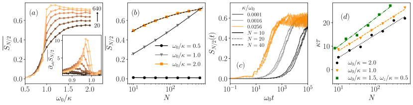
Figure 1: Results of QJ simulations. (a) Long-time average of the half-chain entanglement entropy $\overline{S_{N/2}}$ as a function of $\omega_{0}/\kappa$, for system sizes $N=20,40,80,160,320,640$. In the inset, the numerical derivative of the long-time averaged entanglement entropy highlights the critical point; the peak height grows logarithmically with $N$. (b) Scaling of $\overline{S_{N/2}}$ as a function of $N$ at fixed values of $\omega_{0}/\kappa$. At the critical point, the long-time averaged entanglement entropy grows logarithmically with $N$ (gray triangles). In the phase $\omega_{0}/\kappa<1$ the behavior is area-law (black circles). The scaling in the region $\omega_{0}/\kappa>1$ is sub-logarithmic (orange squares). Numerically, one can fit the curves as $\overline{S_{N/2}}\sim\ln^{\beta}N$ with a non-universal exponent $\beta<1$ ($\beta\sim 0.2$ at $\omega_{0}/\kappa=2$). The exponent decreases when moving away from the critical point. (c) Long-time dynamics of the entanglement entropy for several system sizes and several values of $\kappa/\omega_{0}$. The entanglement entropy grows as $\ln t$ before saturating. (d) Dependence of the saturation time on the system size $N$ (in all cases, $\tau\sim\ln N$).

Despite this large theoretical effort, the experimental evidence of MIPTs is much more limited with only three pioneering experimental works at present [56, 57, 58]. Following a first quantum simulation with trapped ions [56] the scaling close to the critical point has been explored with the IBM quantum processor [57].

There is a fundamental reason that hinders the possibility of observing the measurement-induced phases, and it is known as the post-selection problem. To perform averages of observables along a given trajectory, one should be able to reproduce with sufficient probability the same sequence of random jumps. This is challenging as the probability of reproducing the same trajectory scales to zero exponentially with system size and timescale. It explains why experiments have been limited only to a few sites and considerable efforts were required to increase the lattice length.

Post-selection overhead can be mitigated using space-time duality [59, 60] as it has been experimentally achieved in [58] with the Google processor. Among the novelties of [58] is using the cross-entropy benchmark, a quantum-classical order parameter that combines measurement outcomes to classical post-processing, to detect MIPTs [61, 62, 63]. While, for a perfect detector, this quantity allows to overcome the post-selection problem provided one can simulate efficiently the quantum dynamics on a classical computer, the quantum noise of the currently available devices introduces uncontrolled errors that may deteriorate the experimental detectability. It is worth mentioning the proposals of using adaptive quantum circuits [64, 65], i. e., conditioning the evolution on the measurement registry to render the MIPT visible at the average (density matrix) level. However, this approach generally fails as feedback may alter the physical properties of the system and lead to an inequivalent type of transition concerning the original MIPT [66, 67, 68, 69]. The post-selection problem remains a formidable hurdle to overcome, and the search for cases where it can be mitigated is necessary for experimental progress in monitoring quantum many-body systems.

Here we show that the monitored dynamics of an ensemble of atoms driven by a laser field and in the presence of a collective decay is a very promising choice for this aim. As we will see in the rest of the paper, this system undergoes a MIPT as a function of the laser intensity separating two sub-volume law behaviors with the entanglement diverging logarithmically with the system size at the critical point. This setup does not suffer from the post-selection barrier: at most, the overhead required scales only polynomially with the system size.

The system consists of a cloud of $N$ atoms, each behaving as a two-level system with associated Pauli matrices $\hat{\sigma}_{i}^{\alpha}$, $\alpha=x,y,z$ for the $i$-th atom). A description of the setup can be found, for example, in Ref. [70]. In the absence of monitoring, the density matrix of the system, driven by an external laser with collective decay, obeys the Lindblad equation

$$\dot{\hat{\rho}}=\mathcal{L}(\hat{\rho})\equiv-i[\hat{\cal H},\hat{\rho}]+\frac{\kappa}{J}\Bigl{(}\hat{J}_{-}\hat{\rho}\hat{J}_{+}-\frac{1}{2}\{\hat{J}_{+}\hat{J}_{-},\hat{\rho}\}\Bigr{)},$$ (1)

where $\hat{J}_{\alpha}=\sum_{i}\hat{\sigma}_{i}^{\alpha}/2$, $J=N/2$ is the total spin, $\hat{J}_{\pm}=\hat{J}_{x}\pm i\,\hat{J}_{y}$, and $\hat{\cal H}=\omega_{0}\hat{J}_{x}$. The steady state has a phase transition separating a normal from a time-crystal phase [71, 72, 73]. The dynamic governed by Eq. (1) was recently realized experimentally [70]. To analyze the MIPT at the trajectory level, one should specify the type of monitored dynamics that will be considered, i. e., the unraveling of the Lindblad dynamics in Eq. (1) [74, 75]. We will first study the case of quantum jumps (QJ) and then the case of continuous monitoring, i. e., the quantum state diffusion (QSD). We quantify the entanglement in the steady state through the entanglement entropy and the quantum Fisher information.

Quantum jumps — In this case, the system evolves according to a (smooth) effective non-Hermitian Hamiltonian $\hat{\mathcal{H}}_{\text{nj}}=\hat{\mathcal{H}}-i\,(\kappa/2J)\hat{J}_{+}\hat{J}_{-}$, interrupted, at random times, by quantum jumps when the wavefunction $\ket{\psi(t)}$ changes abruptly as

$$\ket{\psi(t_{+})}=\frac{\hat{J}_{-}\ket{\psi(t_{-})}}{\sqrt{\bra{\psi(t_{-})}\hat{J}_{+}\hat{J}_{-}\ket{\psi(t_{-})}}}.$$ (2)

In a time-interval $\delta t$, jumps occur with a probability $\delta p=\kappa\delta t\langle\hat{J}_{+}\hat{J}_{-}\rangle/J$. Details of the numerics are given in [76].

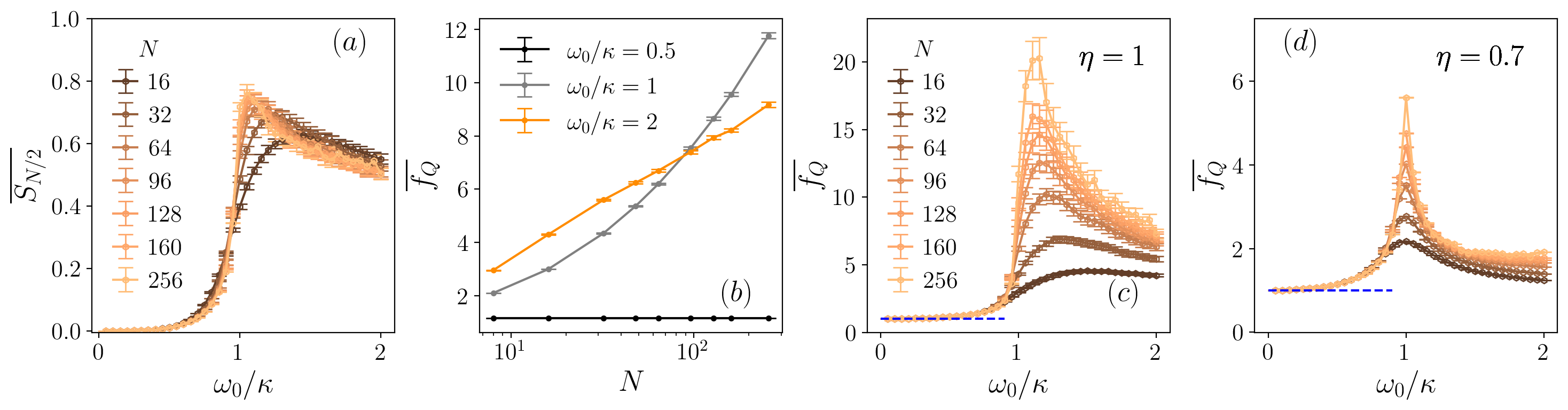
Figure 2: Results of QSD simulations. (a) Long-time averaged entanglement entropy $\overline{S_{N/2}}$ as a function of $\omega_{0}/\kappa$ for various system sizes $N$. The entanglement develops a peak at the critical point $\omega_{0}=\kappa$. (b) Scaling of $\overline{f_{Q}}=\overline{F_{Q}}/N$ as a function of $N$ at the fixed values of $\omega_{0}/\kappa$. At the critical point, the long-time averaged Fisher density grows $\propto\sqrt{N}$ (grey line). In the phase $\omega_{0}<\kappa$, $\overline{f_{Q}}$ saturates to the constant $1$ (black line). For $\omega_{0}>\kappa$, the Fisher density scales logarithmically with the system size. Therefore, the system is multipartite entangled at the critical point and in the non-trivial phase. As discussed in the text, we compare the Fisher density for (c) efficient ($\eta=0$) and (d) inefficient detectors ($\eta=0.7$). The blue-dashed line is the constant value $\overline{f_{Q}}=1$. While quantitative changes are present, the qualitative features of the phase diagram are preserved.

A quantifier of the entanglement present in the wavefunction $\ket{\psi(t)}$ is the entanglement entropy $S_{A}$. Given a bipartition of the system into two subsystems, $A$ and $B$, the entanglement entropy is $S_{A}(\ket{\psi(t)})=-\mbox{Tr}_{A}(\hat{\rho}_{A}\ln\hat{\rho}_{A})$, where $\hat{\rho}_{A}=\mbox{Tr}_{B}\ket{\psi(t)}\bra{\psi(t)}$ is the partial trace over the degrees of freedom of subsystem $B$. We will consider balanced partitions with $N_{A}=N_{B}=N/2$, and the entanglement entropy at long times is then averaged over the quantum trajectories and over the time domain $\overline{S_{N/2}}\;$.

In Fig. 1(a), we plot the averaged entropy $\overline{S_{N/2}}$ as a function of $\omega_{0}/\kappa$ for several values of $N$. In the symmetry-unbroken (small $\omega_{0}$) phase, the half-chain entanglement entropy is essentially independent of $N$: The system is in an area-law phase. An anomaly develops near $\omega_{0}/\kappa\sim 1$ (in this system the MIPT coincides with the transition from a normal to a time-crystal phase [71]). The singularity is clearly visible in the inset of Fig. 1(a). The derivative of $\overline{S_{N/2}}$ has a logarithmic divergence of the peak height with $N$. At the critical point, the entanglement diverges logarithmically as shown in Fig. 1(b). For ${\omega_{0}/\kappa>1}$ the entropy grows more slowly with $N$. From the numerics, a good fit is obtained with $\overline{S_{N/2}}\sim\ln^{\beta}N$ with a non-universal exponent $\beta<1$ that decreases moving away from the transition. In the limit $\omega_{0}/\kappa\gg 1$, $\beta$ tends to zero. A more careful inspection based on the data shown in panels (c) and (d) of Fig. 1 (the entropy grows as $\ln t$ up to a saturation time that depends logarithmically on $N$) suggests $\overline{S_{N/2}}\sim\ln\ln N$. Sub-extensive phases in long-range circuits have been discussed in [77, 78, 79, 80, 81, 82].

Having established the existence and location of a MIPT in this model, it is important to estimate the overhead that we should expect from the unavoidable post-selection in a brute-force experiment. The system analyzed here is free from the post-selection problem. Because of the collective nature of the jumps, a quantum trajectory can be represented as a binary string with a record of the sequence of jumps (once a time-bin has been fixed). The probability of generating the same trajectory thus scales as $2^{-\tau}$ with $\tau$ of the order of the saturation time. For ${\omega_{0}/\kappa<1}$, $\tau$ is independent on $N$ [76]. In the sub-extensive regime ${\omega_{0}/\kappa>1}$ and at the critical point ${\omega_{0}/\kappa=1}$, the saturation time grows logarithmically with the system size,

$$\tau\sim a\log N+b,$$ (3)

see Fig. 1(d) ($a,b$ constants depending on $\omega_{0}/\kappa$). The logarithmic scaling of the saturation time is a signature of collective dissipation [83]. A simple estimate can be obtained obtained from the imaginary part of the non-Hermitian Hamiltonian (details are provided in  [76]). Combining the behaviour of $\tau$ discussed above, it is straightforward to conclude that the probability of occurrence of a given trajectory is independent on the system size for $\omega_{0}/\kappa<1$ and only power-law decaying, $N^{-\gamma}$, in the opposite regime (with $\gamma$ weakly dependent on the coupling constants). The monitored dynamic of the system we consider is thus free from the post-selection problem. This applies to a class of long-range interacting spin-systems with collective decay. We added an all-to-all term to the Hamiltonian of the form ${\cal H}_{z}=\omega_{z}J^{2}_{z}$ and the scaling of the saturation time, shown in Fig. 1(d) green dots, is still logaritmic with the system size. We also considered the case of power-law decay exchange interaction among the spins. In this case, due to the absence of permutational invariance, we can consider much more modest system sizes. The results are reported in [76]. As long as the interaction is sufficiently long-range the dynamics remains post-selection-free (for comparison in  [76] we also show the simulation for the short-range case where this is not the case).

Quantum state diffusion — The enormous advantage of this setup, as shown in the quantum jump unraveling, is also present when the monitoring is not ideal. We will discuss this aspect in the following paragraph where we will analyze the case of continuous monitoring where the evolution of the atomic cloud is governed by quantum state diffusion [84, 3]. The quantum state diffusion arises as the continuous limit of the quantum jump evolution, and is described by the stochastic Schrödinger equation [2]

$$d\hat{\rho}_{\mathrm{w}}=\mathcal{L}(\hat{\rho}_{\mathrm{w}})+\sqrt{\frac{\kappa\eta}{J}}dW(\hat{J}_{-}\hat{\rho}_{\mathrm{w}}+\hat{\rho}_{\mathrm{w}}\hat{J}_{+}-2\langle\hat{J}_{x}\rangle\hat{\rho}_{\mathrm{w}})$$ (4)

where $dW$ is a Gaussian Îto noise with $\overline{dW}=0$ and $dW^{2}=dt$. In Eq. (4) we have introduced the detector efficiency $\eta\in[0,1]$ to treat the effect of noise: $\eta=1$ corresponds to a perfect detector and $\eta<1$ describe imperfect detection, with the limit $\eta=0$ implying no trajectory resolution. Eq. (4) provides a different unraveling of the Lindblad equation in Eq. (1) since $\hat{\rho}=\overline{\hat{\rho}_{\mathrm{w}}}$, and describes a system coupled to a homodyne detector, a framework of experimental relevance in current platforms [85]. Crucially, the homodyne current

$$dI_{t}=\frac{\kappa}{J}\langle\hat{J}_{x}\rangle+\sqrt{\frac{\kappa\eta}{J}}dW$$ (5)

is experimentally detectable, with important consequences for the observability of the measurement-induced transition (see below).

When $\eta=1$ the monitoring is perfect, the purity of an initial state is preserved in the dynamic. In this case, the entanglement entropy is a sensitive measure of quantum correlations in the system. In Fig. 2(a) we present the average entanglement entropy varying $\omega_{0}/\kappa$ and for various system sizes. For $\omega_{0}<\kappa$ the entanglement behaves qualitatively as for the quantum jump evolution [cf. Fig. 1(a)]. Yet, for $\omega_{0}>\kappa$ the available system sizes demonstrate a saturation to a constant value, hence an area-law phase. This is not surprising: the quantum state diffusion is a different unraveling of the Lindblad equation Eq. (1) that is more prone to destroy entanglement, i. e., the infinite click limit of the quantum jump evolution. Remarkably, the phase transition occurs still at $\omega_{0}=\kappa$, where $\overline{S_{N/2}}$ develops a peak.

Realistic experiments have $\eta<1$ due to decoherence to the environment, and Eq. (4) leads to mixed states, potentially altering the entanglement properties of the state [86, 87, 88, 89, 90]. For instance, the von Neumann entropy is not an entanglement measure in this situation, as it also embodies classical correlations. Therefore, to consider perfect and imperfect detectors on the same foot, we study the quantum Fisher information (QFI), a measure of multipartite entanglement valid for pure and mixed states [91, 92, 93, 94, 95, 96, 97]. The quantum Fisher information is

$$F_{Q}(\hat{\rho}_{\mathrm{w}})=\max\mathrm{eigval}(M)$$ (6)

where the matrix $M_{\alpha,\beta}=2\sum_{k,l}\Lambda_{k,l}\langle k|\hat{J}_{\alpha}|l\rangle\langle l|\hat{J}_{\beta}|k\rangle$ is defined for the decomposition $\hat{\rho}_{\mathrm{w}}=\sum_{k}\lambda_{k}|k\rangle\langle k|$ and $\Lambda_{k,l}=(\lambda_{k}-\lambda_{l})^{2}/(\lambda_{k}+\lambda_{l})$ . Eq. (6) gives a bound to the multipartite entanglement entropy: if the Fisher density $f_{Q}\equiv F_{Q}/N$ is (strictly) larger than some divider $k$ of $L$, then the state contains entanglement between $(k+1)$ parties. We note that the QFI is non-linear in the density matrix, hence $\overline{F_{Q}(\hat{\rho}_{\mathrm{w}})}\neq F_{Q}(\overline{\hat{\rho}_{\mathrm{w}}})$. We first discuss the average QFI density $\overline{f_{Q}}$ in the limit $\eta=1$. In Fig. 2(b) we show the system size scaling of $\overline{f_{Q}}$ in the normal phase, critical point, and boundary time crystal phase. In the former, the fisher density saturates to the constant value $\overline{f_{Q}}=1$, signaling that the system is close to a product state. For $\omega_{0}>\kappa$ the Fisher density presents a logarithmic scaling in system size [76]. It follows that this phase exhibits area-law entanglement and logarithmic multipartite entanglement . At the critical point, a polynomial fit demonstrates $\overline{f_{Q}}\sim N^{1/2}$. This fact reveals enhanced multipartite entanglement at the critical point. In Fig. 2(c) we summarize the behavior of the Fisher density for various system sizes and along the phase diagram for the perfect detector ($\eta=1$). Importantly, the salient points of the above discussion are robust against noisy contribution. In Fig. 2(d) we show that the phases and the peak of $\overline{f_{Q}}$ at the critical point are qualitatively unaltered for efficiency rate $\eta=0.7$. Further decreasing $\eta$ we would get close to the Lindblad framework Eq. (1), where the QFI has been computed in [100, 101]. This discussion shows that experimental detection is feasible in the atomic systems of interest. In the next section, we propose an experimental implementation for the MIPT based on driven atomic gases and one on homodyne detection.

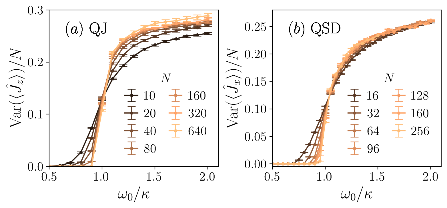
Figure 3: (a) Rescaled trajectory variance of $\langle\hat{J}_{z}\rangle$ for various system sizes and along the phase diagram for the quantum jump evolution. The trajectory histogram of $\langle\hat{J}_{z}\rangle$ is experimentally observable, cf. Ref. [70]. (b) Rescaled trajectory variance of $\langle\hat{J}_{x}\rangle$ for the quantum state diffusion. This quantity is directly obtainable from the homodyne current [2].

Experimental implementation — The model under study here has been recently realized in trapped atomic gases coupled to a mode of the free space electromagnetic environment [102, 70]. In the sub-wavelength regime, a fraction of the atoms share the same diffraction mode and experience a collective decay, as described by the jump operator in Eq. (2). The effective atom number can be tuned in the experiment by changing the geometry of the setup [70]. In a single-shot experiment the number of emitted photons in two orthogonal directions is measured, giving access to the quantum jumps and their statistics. In particular, by monitoring the intensity of the light emitted in the direction perpendicular to the cloud it is possible to access the population of the atomic excited states, $\langle\hat{J}_{z}\rangle$, and its statistics. The polynomial cost of post-selection in this system suggests that reconstructing the trajectory histogram of this observable, as done in experiments with single qubits [103, 104], could be doable. In Fig. 3(a), we compute the variance of the collective spin magnetization, showing a sharp transition at $\omega_{0}/\kappa=1$. An even more direct signature of the transition can be obtained by performing homodyne detection and measuring the variance of the homodyne current. From Eq. (5) we have indeed that $\overline{dI_{t}^{2}}\sim\overline{\langle\hat{J}_{x}\rangle^{2}}$. Hence from the first two moments of $dI_{t}$ we can reconstruct the variance of $\langle\hat{J}_{x}\rangle$ that exhibits a sharp transition at $\omega_{0}/\kappa=1$, cf. Fig. 3(b).

Collective dissipative processes such as those at play here can be naturally engineered in other platforms such as atoms coupled to a cavity mode [105] or qubits collectively coupled to a microwave resonator [106] or a waveguide [107]. Similar phenomenology is expected also in other models of dissipative time-crystals as, for example, in [108].

Conclusions — In this Letter, we showed that a monitored ensemble of atoms, driven by a laser field and in the presence of a collective decay, undergoes a measurement-induced phase transition. The detection of this transition does not suffer from the post-selection problem and can be observed in existing experimental platforms [70, 85]. We analyzed the critical properties of the entanglement entropy and the Fisher information for two different types of monitoring, quantum jumps and quantum state diffusion. Arguably, this behavior is generic in systems with underlying semiclassical dynamics.

Supplemental Material:
Post-selection-free Measurement-Induced Phase Transition in Driven Atomic Gases with Collective Decay

In this Supplemental Material, we discuss: details on the numerical implementation for the stochastic Schrödinger equations considered, additional numerical details, and a phenomenological argument for the saturation time logarithmic in system sizes. Moreover, we study an interacting model with power-law decaying $ZZ$ interactions and demonstrate that the results of the main text are not fine-tuned since they hold whenever the interactions are sufficiently long-ranged.

Appendix 1 Numerical implementation

We simulate the quantum jump (QJ) evolution and the quantum state diffusion (QSD) with exact numerical methods that exploit the permutation symmetry of the system. Indeed, the operator $\hat{J}_{\alpha}$ for $\alpha=x,y,z$ are invariant under exchanges of its constituent. Consequently, the wave function complexity is restricted from the full $2^{N}$-dimensional Hilbert space to the subspace $N+1$ generated by the Dicke states [109]. Given the permutationally symmetric pure state $|\Psi\rangle$ (or $\hat{\rho}=|\Psi\rangle\langle\Psi|$), we compute the entanglement entropy as described in Refs. [110, 111, 112]. The quantum Fisher information is obtained by explicitly evaluating Eq. (7) on the given density matrix $\hat{\rho}$. We now present additional details for the implementation and the choice of hyperparameters considered. We start from the fully polarized Dicke state, but we have tested that the stationary state properties are independent of the initial state.

Quantum jump evolution — For the QJ setup, we simulate the system dynamics in the Dicke basis. In the figures of the main text, averages are computed over $\mathcal{N}=1000$ trajectories using an integration time step of $\kappa\delta t=0.002/N$, which is enough to achieve convergence for all analyzed system sizes. We compute the infinitesimal time-evolution operator of the “no jump” phase,

$$\hat{U}(\delta t)=e^{-i\hat{\mathcal{H}}_{\text{nj}}\delta t},$$ (S1)

using the Padé approximation technique implemented in the expokit library [113], and propagate the state by repeated applications of $\hat{U}(\delta t)$. See the main text for the definition of $\hat{\mathcal{H}}_{\text{nj}}$. We then use the waiting-time distribution algorithm to determine the occurrence of quantum jumps [114]. In particular, the algorithm works as follows: A random number $r$ is extracted from the uniform distribution $\mathcal{U}([0,1])$. The system state is propagated using the time evolution operator of Eq. (S1). Since $\hat{\mathcal{H}}_{\text{nj}}$ is non-Hermitian, the norm of the time-evolved state decreases in time, resulting in an unnormalized state $\ket{\tilde{\psi}(t)}$. At $t=t^{*}$, where $\braket{\tilde{\psi}(t^{*})}{\tilde{\psi}(t^{*})}=r$, a quantum jump occurs and the system state becomes Eq. (2) of the main text. A new random number $r$ is extracted and the algorithm is repeated until the the state is propagated to the final time.

We evolve our systems up to $\kappa T=400$ and compute the long-time averaged half-chain entanglement entropy as

$$\overline{S_{N/2}}=\frac{1}{\Delta T}\int_{T-\Delta T}^{T}S_{N/2}(t)\,dt,$$ (S2)

with $\kappa\Delta T=100$.

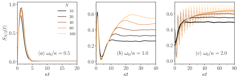
Figure S1: QJ simulations. Dynamics of the half-chain entanglement entropy $S_{N/2}(t)$ for several values of $N$. (a) $\omega_{0}/\kappa=0.5$. (b) $\omega_{0}/\kappa=1.0$. (c) $\omega_{0}/\kappa=2.0$. In (c), transparent lines are real dynamics and solid lines are Gaussian-filtered data with radius $\sigma=20$.

Quantum state diffusion — For the QSD setup, we study the evolution of the density matrix with methods analogous to the quantum jump evolution. At each time step $\delta t$, we exponentiate the dynamical evolution in Eq. (5) using the Padé approximation technique in the expokit library [113]. Importantly, because of the Îto rules, the dynamical generator is [2]

$$\hat{V}_{t}=V_{0}e^{-i\hat{{\cal H}}\delta t-\frac{\kappa\delta t}{J}\left(\hat{J}_{x}\hat{J}_{-}-2\hat{J}_{-}\langle\hat{J}_{x}\rangle_{t}\right)+\sqrt{\frac{\kappa\eta}{J}}dW\hat{J}_{-}},$$ (S3)

with $V_{0}$ a normalization constant, and the density matrix is given by $\hat{\rho}_{\mathrm{w},t+\delta t}=\hat{V}_{t}\hat{\rho}_{\mathrm{w},t}\hat{V}^{\dagger}_{t}/\mathrm{tr}(\hat{V}_{t}\hat{\rho}_{\mathrm{w},t}\hat{V}^{\dagger}_{t})$. In this case, the complexity is rescaled from $2^{N}\times 2^{N}$ to $(N+1)\times(N+1)$. For the simulation presented in the main text, we consider $\delta t=5\times 10^{-3}$ that is sufficient for convergence, as we have tested considering $\delta t=10^{-2}$ and $\delta t=10^{-4}$ giving quantitatively stable results. We consider $\mathcal{N}=1000$ realizations for $N\leq 96$, $\mathcal{N}=250$ for $N=128,160$ and $\mathcal{N}=100$ for $N=256$. The maximum time evolution is $T=400/\kappa$, and the average over the trajectories and the variance are obtained over the times $t\geq 300/\kappa$ and all quantum trajectories.

Appendix 2 Additional numerical results

We complement the numerical findings in the main paper with additional data.

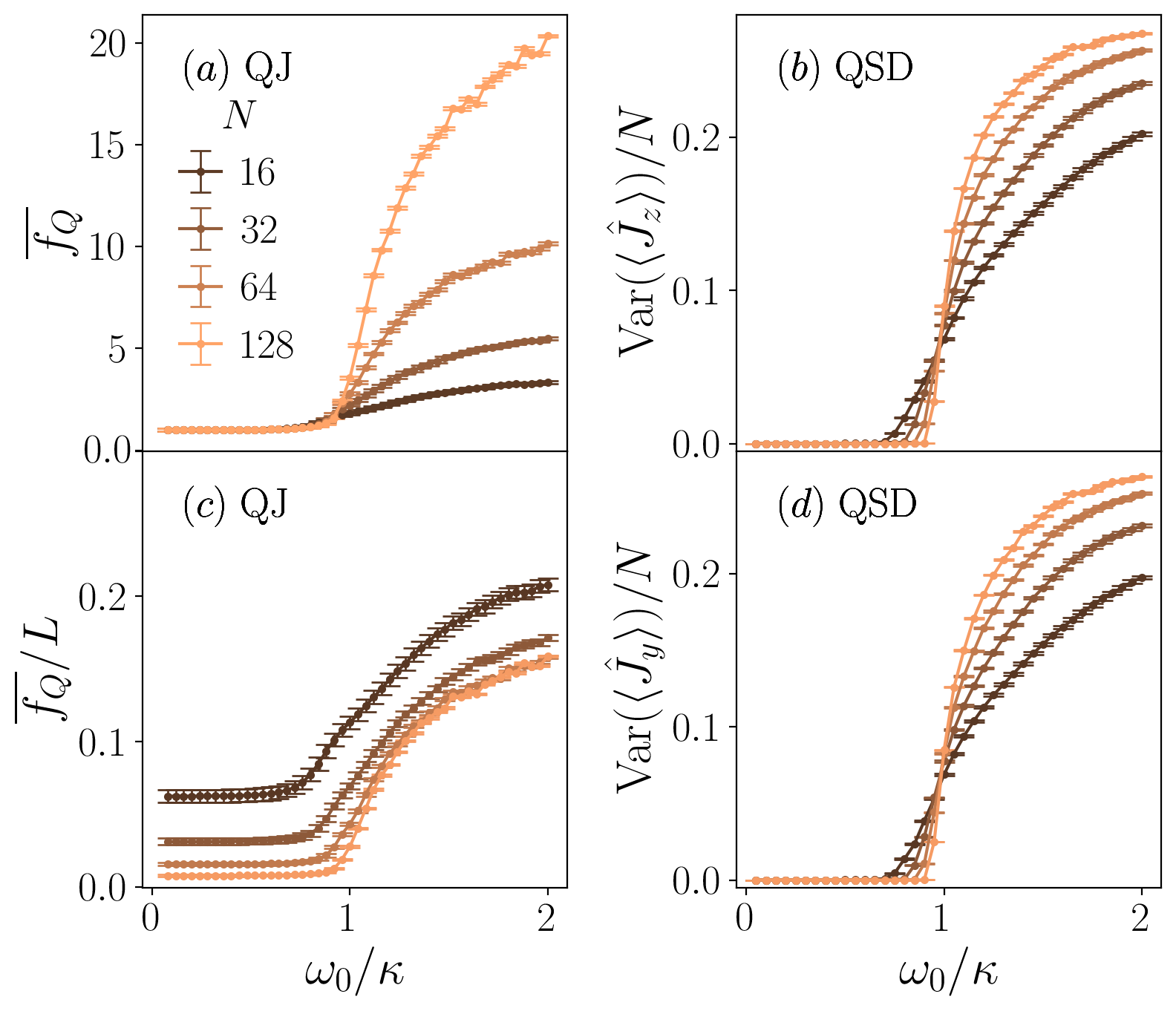
Figure S2: (a) Average Fisher density for the quantum jump evolution at varying values of $\omega_{0}/\kappa$ and system sizes $N$. The normal phase and the time crystal phase correspond to $\overline{f_{Q}}\simeq 1$ and $\overline{f_{Q}}\simeq N$ respectively. We highlight this scaling by plotting $\overline{f_{Q}}/N$ in (c). Rescaled variance of the operator $\hat{J}_{z}$ (b) and $\hat{J}_{y}$ (d) over the trajectories. Both these quantifier develop a sharp transition at the critical point $\omega_{0}=\kappa$.

First, we present other numerical results for the early-time quantum jump evolution of the half-system entanglement entropy averaged over $\mathcal{N}=10000$ trajectories. These results are presented in Fig. S1. Panel (a) demonstrates that the dynamic is rapidly saturating in the normal phase (exemplified by $\omega_{0}/\kappa=0.5$) to a value close to zero. The state indeed is close to an eigenstate of $\hat{J}_{-}$ with low quantum information encoded. The saturation time is independent on $N$. Conversely, panel (c) shows the oscillatory effect that characterizes the time-crystal phase of the system, as presented for $\omega_{0}/\kappa=2$. These regimes are separated by the transition at $\omega_{0}=\kappa$, where a non-trivial scaling dynamics is observed, cf. panel (b).

In order to compute the saturation time $\tau$, we proceed in two different ways for $\omega_{0}/\kappa=1$ and $\omega_{0}/\kappa>1$. At the critical point $\omega_{0}/\kappa=1$, we evaluate the entanglement entropy at the plateau as in Eq. (S2), we then compute the intersection between this value and the crescent branch of $S_{N/2}(t)$ and use this as an estimate of $\tau$. In the time-crystal phase, we use a Gaussian filter with radius $\sigma=20$ to filter out the time crystal oscillations and reduce the dynamics to an asymptotic saturation to $\overline{S_{N/2}}$ according to the law $S_{N/2}(t)=a+b\exp(-t/\tau)$, and estimate $\tau$ by fitting the filtered data. The results of our analysis are reported in Fig. 1(d) of the main text.

Furthermore, we study the quantum Fisher information of the quantum jump unraveling in Fig. S2(a). As we see, the QFI density $\overline{f_{Q}}$ separates a trivial phase ($\overline{f_{Q}}\simeq 1$) at $\omega_{0}<\kappa$ from a maximally multipartite phase at $\omega_{0}>\kappa$. To highlight that $\overline{f_{Q}}\sim N$ we plot the rescaled $\overline{f_{Q}}/N$ in Fig. S2(c). Already for $N=64$, this quantity saturates to a limit curve, highlighting the robustness of the phase. This shows the quantum jump evolution has an inequivalent multipartite entanglement pattern compared to the quantum state diffusion, cf. main text.

Lastly, we study the variance of $\langle\hat{J}_{z}\rangle$ and $\langle\hat{J}_{y}\rangle$ in the quantum state diffusion, see Fig. S2(b) and (d) respectively. While these objects are more involved from an experimental perspective compared to $\mathrm{Var}(\langle\hat{J}_{x}\rangle)$, cf. main text, they also reveal a sharp transition at the critical point $\omega_{0}/\kappa$. In particular, the variance over the $z$-direction reveals qualitatively similar features to the QJ case, cf. Fig. 3 in the main text.

2.1 Saturation Time

The logarithmic scaling of the saturation time is a signature of collective dissipation [83]. A simple estimate can be obtained by assuming that the coherent drive pushes the system at the top of the Dicke ladder while the collective dissipation drives the system down the ladder from a state $M$ to $M-1$ by emitting a photon through a quantum jump. The typical time scale for this process can be obtained from the imaginary part of the non-Hermitian Hamiltonian $\Gamma_{M,M-1}=(\kappa/2J)\langle J_{+}J_{-}\rangle=(\kappa/2J)(J+M)(J-M+1)$. The saturation time is given by summing over the jump events $\tau\sim\sum_{M}1/\Gamma_{M,M-1}$. For single particle jumps, independent on the state $M$ of the system, this would give $\Gamma\sim\kappa$ as expected for independent Poisson processes and a saturation time $\tau\sim N$. The key point is that in our case the emission is a correlated process, i. e., its rate depends on how many jumps have occurred before through $\Gamma_{M,M-1}$, and emission gets faster as the system goes down in the ladder. A simple calculation gives

$$\tau =\frac{2J}{\kappa}\sum_{M=J}^{-J+1}\frac{1}{(J+M)(J-M+1)}=$$ (S4)

$$=\frac{4J}{\kappa(N+1)}\sum_{M=J}^{-J+1}\left(\frac{1}{J+M}+\frac{1}{J-M+1}\right)=$$ (S5)

$$=\frac{8J}{\kappa(N+1)}\sum_{s=1}^{N}\frac{1}{s}$$ (S6)

which, in the large $N$ limit, scales as $\tau\sim\ln N$. We note that the above argument is approximate in that the coherent drive is only used to prepare the state at the top of the ladder, but does not enter the saturation time — this should work in the strong drive regime $\omega_{0}\gg\kappa$.

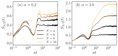
Figure S3: Dynamics of the half-chain entanglement entropy $S_{N/2}(t)$ for the power-law model [Eq. (S7)]. (a) $\alpha=0.2$, long-range regime. (b) $\alpha=3.0$, short-range regime. Parameters: $\omega_{0}/\kappa=1.5$, $\omega_{z}/\kappa=0.5$.

2.2 Power-law interacting model

In this section, we consider a generalization of the model presented in the main text. We use it to demonstrate that the results therein are robust with respect to perturbations of the considered model, provided the resulting Hamiltonian is sufficiently long-range. We consider the following Hamiltonian,

$$\hat{\mathcal{H}}=\omega_{0}\hat{J}_{x}+\frac{\omega_{z}}{\mathcal{Z}_{\alpha,N}}\sum_{j>i}\frac{\hat{\sigma}^{z}_{i}\hat{\sigma}^{z}_{j}}{{d(i,j)}^{\alpha}},$$ (S7)

where $\omega_{z}$ denotes the interaction strength, $d(i,j)=\min(\lvert i-j\rvert,N-\lvert i-j\rvert)$ is the distance between sites $i$ and $j$ along the chain (with periodic boundary conditions) and the exponent $\alpha$ determines the interaction range. The Kac normalization factor $\mathcal{Z}_{\alpha,N}=N^{-1}\sum_{i\neq j}{d(i,j)}^{-\alpha}$ ensures the Hamiltonian is extensive in the thermodynamic limit for all values of $\alpha$. In particular, the infinite-range limit $\alpha=0$ is equivalent to the Lipkin-Meshkov-Glick model (considered in the main text), while the opposite limit $\alpha=\infty$ corresponds to the transverse-field Ising model with nearest-neighbor interactions. The $\alpha<1$ regime is denoted as long-range regime: in the thermodynamic limit, the model behaves as its infinite-range limit $\alpha=0$. Larger values of $\alpha$ result in a short-range model instead. Thus, this Hamiltonian allows us to tune the interaction range and continuously depart from the infinite-range model considered in the main text.

On top of this model, we add collective dissipation as done previously and study the dynamics of the half-chain entanglement entropy $S_{N/2}$ following the quantum jump unravelling, for different values of $\alpha$. Due to the fact that the Hamiltonian is no longer $\mathrm{SU}(2)$-symmetric, only small systems are amenable to simulations via exact diagonalization in the full Hilbert space [$N\sim O(10)$], which is the approach we follow here. We focus our attention on $\omega_{0}/\kappa=1.5$, $\omega_{z}/\kappa=0.5$, $\alpha\in\left\{0.2,2.0\right\}$. The initial state is the fully polarized Dicke state; results are averaged over $\mathcal{N}=1000$ trajectories.

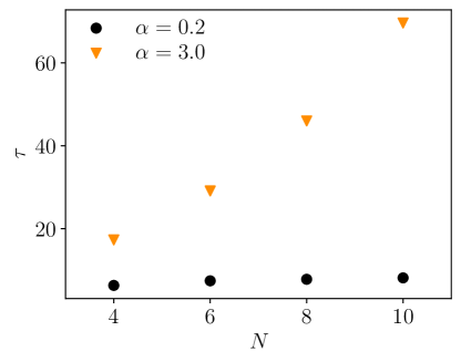
Figure S4: Saturation time $\tau$ versus $N$ in the power-law model [Eq. (S7)] for different interaction ranges. Parameters: $\omega_{0}/\kappa=1.5$, $\omega_{z}/\kappa=0.5$.

In Fig. S3 we plot $S_{N/2}(t)$ versus $t$ for the two considered values of $\alpha$. In both cases, the entanglement entropy reaches a plateau at long times. However, the important difference to remark between the two cases is that the saturation time $\tau$ at which the plateau is reached scales very differently with the system size. This fact is highlighted in Fig. S4, where the difference between the two regimes is evident already at these very small sizes. Remarkably, in the long-range regime we observe features similar to the infinite-range limit, i. e., a very weak dependence of $\tau$ from the system size $N$, which is compatible with the logarithmic scaling observed in the main text for the infinite-range model where much larger system sizes are accessible with numerical simulations. Thus, we conclude that, in the long-range regime, the system remains free from the postselection problem. By contrast, when $\alpha$ is decreased and the model becomes short-ranged, this conclusion no longer holds as the saturation time scales more rapidly with $N$.