When Does Bottom-up Beat Top-down in Hierarchical Community Detection?

Abstract

Hierarchical clustering of networks consists in finding a tree of communities, such that lower levels of the hierarchy reveal finer-grained community structures. There are two main classes of algorithms tackling this problem. Divisive (top-down) algorithms recursively partition the nodes into two communities, until a stopping rule indicates that no further split is needed. In contrast, agglomerative (bottom-up) algorithms first identify the smallest community structure and then repeatedly merge the communities using a linkage method. In this article, we establish theoretical guarantees for the recovery of the hierarchical tree and community structure of a Hierarchical Stochastic Block Model by a bottom-up algorithm. We also establish that this bottom-up algorithm attains the information-theoretic threshold for exact recovery at intermediate levels of the hierarchy. Notably, these recovery conditions are less restrictive compared to those existing for top-down algorithms. This shows that bottom-up algorithms extend the feasible region for achieving exact recovery at intermediate levels. Numerical experiments on both synthetic and real data sets confirm the superiority of bottom-up algorithms over top-down algorithms. In particular, a notable drawback of top-down algorithms is their tendency to produce dendrograms with inversions. These findings contribute to a better understanding of hierarchical clustering techniques and their applications in network analysis.

Keywords: Community detection, hierarchical clustering, linkage, stochastic block model.

1 Introduction

A system of pairwise interactions among entities can conveniently be represented by a graph, where the entities of the system are the nodes and the interactions are the edges. Data collected in such form is increasingly abundant in many disciplines, such as in sociology, physics, economics, and biology New (18). Among the various statistical analysis tasks on networks, community detection–grouping nodes with similar connection patterns into clusters–is one of the most important and most studied For (10); AD (22). While partitioning the node set into flat clusters already provides plenty of information on the network, community structures are often hierarchical. For example, in a co-authorship network, we can partition the researchers based on their primary discipline (such as mathematics, physics, computer science, etc.), while each of these fields can be further split into specific sub-disciplines. The sub-division of larger communities into smaller ones is represented by a tree of communities, in which deeper levels of the tree provide finer division of the network.

Hierarchical communities can be inferred using top-down approaches, where the process begins by identifying the largest communities at the highest level of the hierarchy. These communities are then recursively decomposed into smaller sub-communities at lower levels until a stopping rule indicates that further division is unnecessary. For example, some algorithms progressively remove edges with the highest edge-betweenness centrality GN (02) or with the lowest edge-clustering coefficient RCC⁺ (04). Alternatively, some algorithms use spectral clustering for recursive bi-partitioning of the network DHKM (06); BXKS (11); LLB⁺ (22). However, top-down algorithms possess several limitations. Firstly, any clustering errors made at higher levels become locked in and propagate to lower levels, potentially compromising the accuracy of the predicted hierarchy. Secondly, the recursive splittings overlook valuable information by disregarding edges that connect communities at higher levels when dividing lower-level communities. As a result, these approaches may not fully capture the interconnections between communities across different levels of the hierarchy.

In contrast, agglomerative (or bottom-up) algorithms take a different approach by constructing the hierarchical tree of communities from the bottom upwards. These algorithms recursively merge smaller communities to form larger ones. Some bottom-up algorithms, such as the one proposed in BCGH (18); PL (05); CHCL (11), generate a complete dendrogram. A dendrogram is a tree-like structure where the leaves represent individual nodes, and the branches and internal nodes represent the merging of clusters at various levels of similarity. The length or height of the branches in the dendrogram reflects the degree of similarity between the merged clusters. On the other hand, other algorithms, such as greedy schemes focused on maximizing modularity CNM (04); BGLL (08); HSH⁺ (10), produce partial dendrograms, since the leaves are no longer associated with individual nodes but with the bottom communities. An alternative strategy to construct partial dendrograms involves initially inferring the underlying flat communities using a graph clustering algorithm. Subsequently, these communities are merged through a procedure known as linkage CAKMTM (19). This last approach offers flexibility in building the dendrogram by selectively incorporating community merges based on specific criteria.

Establishing theoretical guarantees assessing the performance of HCD algorithms on random graph models is important to compare various HCD algorithms. The Hierarchical Stochastic Block Model (HSBM) is a general model of random graphs with hierarchical communities. This model defines the hierarchical community structure as a rooted binary tree, whose leaves correspond to primitive communities. Each node belongs to a primitive community and interactions among two nodes belonging to communities $a$ and $b$ depend only on the lowest common ancestor between $a$ and $b$ on the hierarchical tree.

Previous research on SBM has demonstrated that when the number of nodes $N$ grows to infinity, the asymptotic recovery of the communities with only a vanishing fraction of misclassified vertices (known as asymptotically almost exact recovery in the literature) is feasible when the average degree of the graph grows arbitrarily slowly MNS (16). Once the communities have been almost exactly recovered, we establish that the linkage procedure accurately reconstructs the hierarchical tree. Notably, this ability to correctly recover the community hierarchy in a regime where the average graph degree is $\omega(1)$ stands in contrast to earlier studies that necessitated stronger growth conditions. For example, earlier works require the node degrees to grow with $N$ at a rate $\Theta(N)$ BXKS (11), $\omega(N^{1/2}\log^{p}N)$ (with $p=1/2$ in CAKMT (17) and $p=2$ in LTA⁺ (16)), and $\omega(\log^{1+p}N)$ (with $p=5$ for DHKM (06) and $p=1+\Omega(1)$ for LLB⁺ (22)).

The asymptotically exact recovery of the communities is the strongest notion of recovery, as it is defined by the ability to correctly identify the entire partition when the number of nodes diverges. The condition for exact recovery exhibits a phase transition phenomenon when the average degree is of the order $\log N$. In the context of hierarchical communities, it is additionally possible to examine exact recovery at the different intermediate levels of the hierarchy. In this study, we rigorously establish the information-theoretic threshold for exact recovery at any intermediate level of the hierarchy. We demonstrate that bottom-up algorithms using the linkage procedure achieve this threshold. Notably, recovering deeper levels is more challenging than recovering higher levels. Previous research in this area showed that recursive spectral bi-partitioning, a top-down algorithm, asymptotically exactly recovers the levels $1$ to $\ell$ of the hierarchy if a set of conditions is respected LLB⁺ (22). However, our work reveals that these conditions are stricter than the information-theoretic threshold. As a result, bottom-up algorithms extend the feasible region of intermediate-level recovery up to the information-theoretic limits.

In our numerical experiments, we employ a bottom-up algorithm that follows a two-step process. We first apply a spectral algorithm on the Bethe-Hessian to infer the underlying primitive communities SKZ (14); DCT (21). Then, we construct the hierarchy using the linkage procedure. To provide a comprehensive comparison, we evaluate this bottom-up algorithm against the top-down approach known as recursive spectral bi-partitioning Lei (20); LLL (21). Our findings on synthetic data sets demonstrate that the bottom-up algorithm achieves exact recovery at intermediate levels up to the information-theoretic thresholds. In contrast, recursive spectral bi-partitioning, while showing good performances, falls short of achieving this level of precision. Furthermore, we illustrate that the dendrogram produced by recursive spectral bi-partitioning can suffer from inversions. Inversions are undesirable characteristics which occur when the clustering algorithm incorrectly positions a lower-level cluster above a higher-level cluster in the dendrogram, distorting the true hierarchical structure. Such inversions can lead to misleading interpretations of the hierarchical relationships within the data.

The paper is structured as follows. Section 2 describes top-down and bottom-up approaches for hierarchical community detection. The main notations are presented in Section 3, in which we also derive conditions for recovering the hierarchy by the linkage algorithm, as well as its robustness to mistakes in the initial clustering. We then investigate the exact recovery at intermediate levels of the hierarchy in Section 4. We discuss these results in light of the existing literature in Section 5. Finally, Section 6 is devoted to the numerical experiments.

Notations

We denote by $[N]$ the set $\{1,\cdots,N\}$, by $\operatorname{Ber}(p)$ a Bernoulli random variable with parameter $p$, and by $\mathrm{Multi}(N,\mathcal{S},\pi)$ a multinomial distribution with $N$ trials, a (finite, discrete) set of possible outcomes $\mathcal{S}$, and a vector of probability $\pi$ such that $\pi_{s}$ is the probability of success of $s\in\mathcal{S}$. The Frobenius norm of a matrix is denoted $\|\cdot\|_{F}$.

The Rényi divergence of order $t\in(0,1)$ of a Bernoulli distribution $\operatorname{Ber}(p)$ from another distribution $\operatorname{Ber}(q)$ is defined as $\operatorname{D}_{t}\left(\operatorname{Ber}(p)\|\operatorname{Ber}(q)\right)=\frac{1}{t-1}\log\left((1-p)^{t}(1-q)^{1-t}+p^{t}q^{1-t}\right)$. When $t=1/2$, this quantity is symmetric and we simply write $\operatorname{D}_{1/2}\left(\operatorname{Ber}(p),\operatorname{Ber}(q)\right)$.

We focus on undirected graphs $G=(V,E)$ whose node set is $V=[N]$ and adjacency matrix $A=\left(A_{ij}\right)\in\{0,1\}^{N\times N}$. For a subset $V_{1}$ of the node set $V$, we denote by $G[V_{1}]$ the subgraph of $G$ induced by $V_{1}$. Finally, we denote by $\mathcal{N}_{\mathcal{T}}$ (resp., $\mathcal{L}_{\mathcal{T}}$) the internal nodes (resp., the leaves) of a tree $\mathcal{T}$. For an internal node $u$ of a rooted $\mathcal{T}$, we denote by $\mathcal{T}[u]$ the sub-tree rooted at $u$. The lowest common ancestor between two nodes $u,v\in\mathcal{T}$ is denoted $\mathrm{lca}(u,v)$.

2 Hierarchical community detection

Many networks present a hierarchical community structure. The primitive communities are a collection of subsets $\mathcal{C}=(C_{1},\cdots,C_{K})$ that partition the original node set $V$ into $K$ disjoint sets. These primitive communities are the leaves of a rooted tree $\mathcal{T}$, and this tree defines the hierarchical relationship between the communities. This section reviews two main strategies for performing hierarchical community detection (HCD).

2.1 Divisive (top-down) algorithms

Divisive (top-down) algorithms start with one single community containing all the nodes. This community is recursively split until a selection rule indicates that no further splits are needed. This can be summarized as follows:

1. apply a selection rule to decide if the community contains sub-communities. If no, stop; if yes, split into two communities;

2. recursively repeat step 1 on each of the resulting communities as long as the selection rule tells you to continue.

Existing works have explored different choices for the stopping rule or the bi-partitioning algorithms DHKM (06); BXKS (11); LLB⁺ (22). In this process, each recursive splitting of the graph loses a large amount of information. Indeed, consider the two clusters $C_{0}$ and $C_{1}$ obtained after the first split. The next step splits $C_{0}$ (resp., $C_{1}$) into two clusters $C_{00}$ and $C_{01}$ (resp., $C_{10}$ and $C_{11}$), based only on the sub-graph $G[C_{0}]$ (resp. $G[C_{1}]$). This implies that the clustering of $C_{0}$ does not take into account the edges from $C_{0}$ to $C_{1}$. If the edge densities between $C_{00}$ and $C_{1}$ are different from the edge densities between $C_{01}$ and $C_{1}$, then this loss of information may perturb the splitting of $C_{0}$.

Furthermore, it is important to note that the resulting tree is unweighted. Although it is possible to compute similarities between pairs of predicted clusters (for example using the edge density between two clusters), there are no guarantees that these similarities will exhibit a monotonous pattern. Consequently, when using a top-down partitioning approach to create a dendrogram representation, it is possible for inversions to occur. These inversions, as we will emphasize in the numerical section, can lead to discrepancies in the hierarchical structure portrayed by the dendrogram.

2.2 Agglomerative (bottom-up) algorithms

Agglomerative hierarchical community detection algorithms construct a sequence of clusterings in an ascending manner, where the dendrogram is formed from its leaves to its root. The initial clustering corresponds to the leaves of the dendrogram, and the hierarchy is progressively built by iteratively merging the most similar clusters.

One approach involves initially assigning each node to a separate community and then merging the clusters that minimize a distance New (04); PL (05); CHCL (11); BCGH (18). Although these methods generate a complete dendrogram, determining the level in the hierarchy where the community structure becomes meaningful is an old yet challenging problem Moj (77); GBW (22).

Another approach consists of first estimating the bottom clusters using a flat (non-hierarchical) graph clustering algorithm. Moreover, in most practical applications, the number of bottom communities $K$ is unknown and has to be inferred as well by the initial clustering algorithm.

The edge density between two node sets $V_{1},V_{2}\subset V$ is

$$\rho\left(V_{1},V_{2}\right)\ =\ \frac{w\left(V_{1},V_{2}\right)}{|V_{1}|\cdot|V_{2}|}\quad\text{ where }\quad w\left(V_{1},V_{2}\right)\ =\ \sum_{i\in V_{1}}\sum_{j\in V_{2}}A_{ij},$$ (2.1)

and defines a similarity measure between two clusters. Let $\widehat{C}_{1},\cdots,\widehat{C}_{\widehat{K}}$ be the clusters initially predicted by the flat graph clustering algorithm. Suppose that at some step of the algorithm, clusters $\widehat{C}_{k_{1}}$ and $\widehat{C}_{k_{2}}$ are the most similar and hence are merged to give a new cluster $\widehat{C}_{k_{1}\cup k_{2}}=\widehat{C}_{k_{1}}\cup\widehat{C}_{k_{2}}$. We have for $\ell\not\in\{k_{1},k_{2}\}$,

$$\rho\left(\widehat{C}_{k_{1}\cup k_{2}},\widehat{C}_{\ell}\right)\ =\ \frac{\left|\widehat{C}_{k_{1}}\right|}{\left|\widehat{C}_{k_{1}\cup k_{2}}\right|}\rho\left(\widehat{C}_{k_{1}},\widehat{C}_{\ell}\right)+\left(1-\frac{\left|\widehat{C}_{k_{1}}\right|}{\left|\widehat{C}_{k_{1}\cup k_{2}}\right|}\right)\rho\left(\widehat{C}_{k_{2}},\widehat{C}_{\ell}\right).$$ (2.2)

Thus, the edge density naturally defines an average-linkage procedure for merging the clusters identified through the initial flat clustering. In particular, this procedure guarantees that the resulting dendrogram will be free from inversions, ensuring a coherent hierarchical structure MC (17). Algorithm 1 provides a concise summary of this process.

Input: Graph $G=(V,E)$, flat graph clustering algorithm algo.

Output: Hierarchical clustering tree $\widehat{\mathcal{T}}$ and its associated bottom clusters $\widehat{C}_{1},\cdots,\widehat{C}_{\widehat{K}}$.

Process:

1. Let $\widehat{\mathcal{C}}=\left(\widehat{C}_{1},\cdots,\widehat{C}_{\widehat{K}}\right)$ be the $\widehat{K}\geq 2$ clusters outputted by algo;

2. For all $k,\ell\in\left[\widehat{K}\right]$ compute $\rho\left(\widehat{C}_{k},\widehat{C}_{\ell}\right)$ as in (2.1);

   while $\left|\widehat{C}\right|\geq 2$ do:

   • Let $\widehat{C}_{k},\widehat{C}_{\ell}\in\operatorname*{arg\,max}\limits_{C\neq C^{\prime}\in\widehat{\mathcal{C}}}\rho\left(C,C^{\prime}\right)$;

   • Let $\widehat{\mathcal{C}}\leftarrow\widehat{\mathcal{C}}\,\backslash\,\left\{\widehat{C}_{k},\widehat{C}_{\ell}\right\}$;

   • For any $C\in\widehat{\mathcal{C}}$ compute $\rho\left(\widehat{C}_{k\cup\ell},C\right)$ as defined in (2.2);

   • Let $\widehat{\mathcal{C}}\leftarrow\widehat{\mathcal{C}}\cup\left\{\widehat{C}_{k\cup\ell}\right\}$.

Return: The tree $\widehat{\mathcal{T}}$ corresponding to the sequence of merges in the while-loop and the bottom communities $\widehat{C}_{1},\cdots,\widehat{C}_{\widehat{K}}$ associated to the leaves of $\widehat{\mathcal{T}}$.

1

Algorithm 1 Bottom-up hierarchical community detection.

3 Tree recovery from the bottom

In this section, we study the asymptotic performance of bottom-up algorithms on a class of random graphs with hierarchical community structures. We define the model in Section 3.1, and we establish the condition for recovering the hierarchical tree from the bottom communities in Section 3.2. Then, we show in Section 3.3 that the average-linkage procedure is robust to errors made in the initial clustering step.

3.1 Hierarchical Stochastic Block Model

The Hierarchical Stochastic Block Model (HSBM) is a class of random graphs whose nodes are partitioned into latent hierarchical communities. Before defining this model formally, let us introduce some notations. Each node $u$ of a rooted binary tree $\mathcal{T}$ is represented by a binary string as follows. The root is indexed by the empty string $\emptyset$. Then, each node $u$ of the tree is uniquely defined by a binary string $u$ that records the path from the root to the node (i.e., $u_{q}=1$ if step $q$ of the path is along the right branch of the split and $u_{q}=0$ otherwise). The depth of node $u$ is denoted by $|u|$ and coincides with its distance from the root. Finally, with this parametrization, the lowest common ancestor $\mathrm{lca}(u,v)$ of two nodes $u,v\in\mathcal{T}$ is simply the longest common prefix of the binary strings $u,v$.

In the following, we denote by $\mathcal{L}_{\mathcal{T}}$ the leaves of the tree $\mathcal{T}$. We will assign each node of the graph $G$ to one leaf of $\mathcal{T}$, and denote by $C_{a}$ the set of nodes assigned to the leaf $a$, which forms the primitive communities $\mathcal{C}=\left(C_{a}\right)_{a\in\mathcal{L}_{\mathcal{T}}}$. Any internal node $u$ of the tree is associated with a super-community $C_{u}$ such that $C_{u}=\cup_{a\in\mathcal{L}_{\mathcal{T}[u]}}C_{a}$ where $\mathcal{L}_{\mathcal{T}[u]}$ denotes the leaves of the sub-tree of $\mathcal{T}$ rooted at $u$. In particular, we have $C_{\emptyset}=V$ and $C_{v}\subset C_{u}$ if $v$ is a child of $u$.

We will suppose that the probability $p_{ab}$ of having a link between two nodes belonging to the primitive communities $C_{a}$ and $C_{b}$ depends only on the lowest common ancestor of $a$ and $b$. We will thus denote the probability $p_{ab}$ by $p(\mathrm{lca}(a,b))$. In an assortative setting, we have $p(u)<p(v)$ if $v$ is a child of $u$. Finally, we need to rule out settings in which the difference $p(v)-p(u)$ decreases too fast with respect to $p(u)$. To avoid this flatness of $p$ issue, we will assume that $\liminf\frac{\left|p(v)-p(u)\right|}{p(u)}>0$ for any child $v$ of a parent $u$.

We can now give the definition of an assortative Hierarchical Stochastic Block Model.

Definition 1.

Let $N$ be a positive integer, $\mathcal{T}$ a rooted binary tree with $K$ leaves, $\pi=(\pi_{a})_{a\in\mathcal{L}_{\mathcal{T}}}$ a probability vector and a function $p\colon\mathcal{T}\to[0,1]$ such that for $u,v\in\mathcal{T}$ we have $p(u)<p(v)$ (assortativity) and $\liminf\frac{p(u)-p(v)}{p(u)}>0$ (non-flat hierarchy) if $v$ is a child of $u$. A Hierarchical Stochastic Block Model (HSBM) is a graph $G=(V,E)$ such that $V=[N]$ and

1. each node $i\in[N]$ is independently assigned to a community $C_{a}$ where $a\sim\mathrm{Multi}(1,\mathcal{L}_{\mathcal{T}},\pi)$;

2. two nodes $i\in C_{a}$ and $j\in C_{b}$ are connected with probability $p(\mathrm{lca}(a,b))$.

An important particular case of HSBM is the Binary Tree SBM (BTSBM), in which the tree $\mathcal{T}$ is full and balanced, and the probability of a link between two nodes in clusters $C_{a}$ and $C_{b}$ depends only on the depth of $\mathrm{lca}(a,b)$, i.e., $p(\mathrm{lca}(a,b))=p_{|\mathrm{lca}(a,b)|}$ for all $a,b\in\mathcal{L}_{\mathcal{T}}$. In particular, the number of communities of a BTSBM is $K=2^{d_{\mathcal{T}}}$, and assortativity implies that $p_{0}<p_{1}<\cdots<p_{d_{\mathcal{T}}}$. We illustrate an HSBM and a BTSBM in Figure 1.

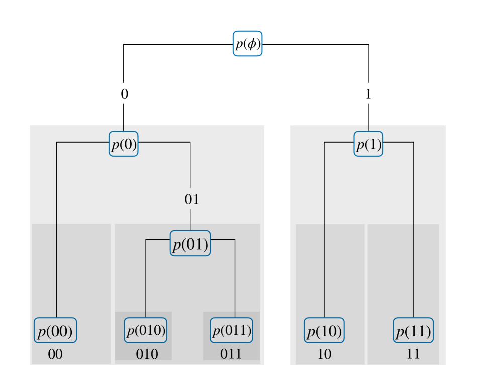
(a) Hierarchical Stochastic Block Model.

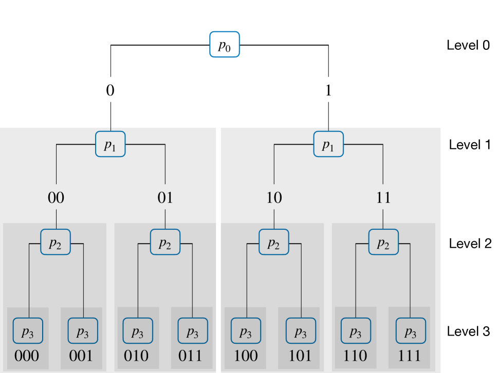
(b) Binary Tree SBM with depth 3.

Figure 1: Examples of an HSBM and a BTSBM, with the binary string representation of each node. The link probabilities are $p(u)$ for the HSBM and $p_{|u|}$ for the BTSBM. The grey-colored rectangles represent the super-communities.

3.2 Tree recovery from the bottom clusters

In this section, we study the recovery of the hierarchical tree $\mathcal{T}$ and the bottom communities $\mathcal{C}=\left(C_{\ell_{1}},\cdots,C_{\ell_{K}}\right)$ associated with the $K$ leaves of $\mathcal{T}$. For an estimator $\widehat{\mathcal{C}}=\left(\widehat{C}_{1},\cdots,\widehat{C}_{K}\right)$ of $\mathcal{C}$, the the number of mis-clustered nodes is

$$\mathrm{loss}\left(\mathcal{C},\widehat{\mathcal{C}}\right)\ =\ \min_{\tau\in\mathcal{S}_{[K]}}\sum_{k=1}^{K}\left|C_{\ell_{k}}\,\Delta\,\widehat{C}_{\tau(k)}\right|,$$ (3.1)

where $B\,\Delta\,C=\left(B\cup C\right)\backslash\left(B\cap C\right)$ denotes the symmetric difference between two sets $B,C\subset V$. The minimum is taken over the set $\mathcal{S}_{[K]}$ of all permutations of $[K]$ since we only recover the bottom communities up to a global permutation of the community labels. We study sequences of networks indexed by the number of nodes $N$ and for which the interaction probabilities may depend on $N$. An estimator $\widehat{\mathcal{C}}$ of $\mathcal{C}$ achieves almost exact recovery if $N^{-1}\mathrm{loss}\left(\mathcal{C},\widehat{\mathcal{C}}\right)=o(1)$ a.s. and exact recovery if $\mathrm{loss}\left(\mathcal{C},\widehat{\mathcal{C}}\right)=o(1)$ a.s.

As the HSBM is a particular case of an SBM with $K=|\mathcal{L}_{\mathcal{T}}|$ communities and link probabilities between communities $\left(p(\mathrm{lca}(a,b)\right)_{a,b\in\mathcal{L}_{\mathcal{T}}}$, the HSBM inherits the recovery conditions obtained for the SBM. Indeed, suppose that $p(u)=a(u)\delta_{N}$ where $\delta_{N}\gg 1$. Then, AS15b ; YP (16) proposed algorithms agnostic to $K$, $\pi$ and $p$ that achieve almost exact recovery as soon as $\delta_{N}\gg N^{-1}$.

The number of edges between two communities $C_{a}$ and $C_{b}$ is binomially distributed with mean $|C_{a}|\cdot|C_{b}|\cdot p_{ab}$. Therefore, if $p_{ab}\gg N^{-2}$, this binomial random variable will be concentrated around its mean and we anticipate to have $\rho(C_{a},C_{b})=(1+o(1))p_{ab}$. This hints that, once the primitive communities are (almost) exactly recovered, the average-linkage procedure will successfully recover the tree from its leaves if the link-probability between different communities is $\omega\left(N^{-2}\right)$. Nonetheless, problems might occur because we compute $\rho(\widehat{C}_{a},\widehat{C}_{b})$ and not $\rho(C_{a},C_{b})$. Indeed, consider the set of node pairs $(i,j)$ such that $i\in C_{a}\cap\widehat{C}_{a}$ and $j\in C_{a}\cap\widehat{C}_{b}$, with $a\neq b$. These node pairs will add noisy terms such as $w\left(C_{a}\cap\widehat{C}_{a},C_{b^{\prime}}\cap\widehat{C}_{b}\right)$, with $b^{\prime}\neq b$, to $w(\widehat{C}_{a},\widehat{C}_{b})$. Therefore, we expect the set of links between $\widehat{C}_{a}$ and $\widehat{C}_{b}$ to contain $p_{ab^{\prime}}\cdot|C_{a}\cap\widehat{C}_{a}|\cdot|C_{b^{\prime}}\cap\widehat{C}_{b}|$ noisy links between $C_{a}\cap\widehat{C}_{a}$ and $C_{b^{\prime}}\cap\widehat{C}_{b}$, versus $p_{ab}\cdot|C_{a}\cap\widehat{C}_{a}|\cdot|C_{b}\cap\widehat{C}_{b}|$ correct links. If $\widehat{\mathcal{C}}$ is consistent, the number of such bad node pairs is small, and hence $p_{ab^{\prime}}\cdot|C_{a}\cap\widehat{C}_{a}|\cdot|C_{b^{\prime}}\cap\widehat{C}_{b}|=o\left(p_{ab^{\prime}}N^{2}\right)$ while $p_{ab}\cdot|C_{a}\cap\widehat{C}_{a}|\cdot|C_{b}\cap\widehat{C}_{b}|=\Theta\left(p_{ab}N^{2}\right)$. Therefore we expect the noise terms to be negligible compared to the correct signal if the probabilities $p_{ab}$ have the same asymptotic scale. This hints at the ability to correctly identify the hierarchy among the communities using the average-linkage procedure if one starts with a consistent estimator of $\widehat{C}$. However, because the predicted clusters $\widehat{\mathcal{C}}$ are correlated with the edges of the graph, rigorous analysis is more involved. We summarize this in the following theorem.

Theorem 1.

Consider an assortative HSBM whose latent binary tree $\mathcal{T}$ has $K=\Theta(1)$ leaves, and suppose that $\pi_{a}>0$ for all $a\in\mathcal{L}_{\mathcal{T}}$. Let $(a(t))_{t\in\mathcal{T}}$ be positive constants (independent of $N$), and $\delta_{N}\gg N^{-1}$ such that $p(t)=a(t)\delta_{N}$. Then, there exists a flat graph clustering algorithm that outputs an almost exact estimator of $\mathcal{C}$. Moreover, the average-linkage procedure correctly recovers the tree $\mathcal{T}$ (starting from $\widehat{\mathcal{C}}$).

We prove Theorem 1 in Appendix A.1. The bottom-up algorithm is Algorithm 1 where the initial clustering is done either by the spectral algorithm of YP (16) or by the agnostic-degree-profiling algorithm of AS15b .

3.3 Robustness of the linkage procedure

In this section, we study the robustness of the linkage procedure to classification errors made by the initial clustering. We suppose that each node has probability $\eta$ to be misclustered, in which case its cluster assignment is modified as follows:

• scenario 1: the misclustered nodes are assigned to a cluster chosen uniformly at random among the clusters that are the closest to their true cluster;

• scenario 2: the misclustered nodes are assigned to a cluster uniformly at random among all clusters (and which could be their true cluster);

• scenario 3: the misclustered nodes are assigned to a cluster chosen uniformly at random among the clusters that are the furthest away from their true cluster.

The resulting bottom clusters under scenarios $s\in\{1,2,3\}$ are denoted $\widetilde{\mathcal{C}}^{s}=\left(\tilde{C}^{s}_{\ell}\right)_{\ell\in\mathcal{L}_{\mathcal{T}}}$. Let $\mathcal{O}$ be the set of misclustered nodes, and $\mathcal{O}^{c}=V\backslash\mathcal{O}$ be the complement of $\mathcal{O}$. We have $C_{a}\cap\mathcal{O}^{c}=\tilde{C}^{s}_{a}\cap\mathcal{O}^{c}$ for all $a\in\mathcal{L}_{\mathcal{T}}$, while a node $i\in C_{a}\cap\mathcal{O}$ is mistakenly clustered in $\tilde{C}^{s}_{b}$ where $b$ is chosen as follows:

$$b\ =\ \begin{cases}\mathrm{Unif}\left(\operatorname*{arg\,max}_{c\in\mathcal{L}_{\mathcal{T}}\backslash\{a\}}|\mathrm{lca}(a,c)|\right)&\text{ in scenario 1 }(s=1),\\ \mathrm{Unif}\left(\mathcal{L}_{\mathcal{T}}\right)&\text{ in scenario 2 }(s=2),\\ \mathrm{Unif}\left(\{c\in\mathcal{L}_{\mathcal{T}}\colon\mathrm{lca}(a,c)=\emptyset\}\right)&\text{ in scenario 3 }(s=3).\\ \end{cases}$$

In the first scenario, the leaf $b$ is uniformly chosen among the leaves whose least common ancestors have the highest depth. This represents a scenario in which mistakes occur solely between similar clusters, and hence this should not handicap the tree reconstruction. In contrast, in the third scenario, the leaf $b$ is chosen among the leaves whose lowest common ancestor with $a$ is the root. This represents an adversarial setting, in which mistakes occur between the least similar clusters, which should heavily handicap the tree reconstruction. The second scenario is an intermediate between the two. The leaf $b$ is uniformly chosen (with the possibility that $b=a$), and hence misclassified nodes are uniformly distributed across all clusters. For each of these scenarios, the following proposition studies the ability of the average linkage in recovering the hierarchical tree from $\widetilde{\mathcal{C}}^{s}$.

Proposition 1.

Let $G$ be a BTSBM whose latent binary tree $\mathcal{T}$ has depth $d_{\mathcal{T}}\geq 2$. Suppose that $\pi_{a}=1/K$ for all $a\in\mathcal{L}_{\mathcal{T}}$ and that $\min\limits_{u\in\mathcal{T}}p(u)\gg N^{-2}$. Suppose that the probability of misclustering $\eta$ verifies $\eta<0.5$, and let $\widehat{\mathcal{T}}^{s}$ be the hierarchical tree obtained by the average-linkage procedure from $\widetilde{\mathcal{C}}^{s}$. The following holds:

1. $\widehat{\mathcal{T}}^{1}=\mathcal{T}$ whp;

2. $\widehat{\mathcal{T}}^{2}=\mathcal{T}$ whp;

3. let $\bar{p}_{1}=\frac{1}{2^{d-1}}\left(p_{d}+\sum_{k=1}^{d-1}2^{k-1}p_{d-k}\right)$ and $\eta_{-}=\frac{p_{d-1}+\bar{p}_{1}-2p_{0}-\sqrt{(\bar{p}_{1}-p_{d-1})(\bar{p}_{1}-p_{0})}}{p_{d-1}+3\bar{p}_{1}-4p_{0}}$. We have $\widehat{\mathcal{T}}^{3}=\mathcal{T}$ whp if one of these two conditions is verified:

   1. $\bar{p}_{1}<p_{d-1}$;

   2. $\bar{p}_{1}\geq p_{d-1}$ and $\eta<\eta_{-}$.

The proof of Proposition 1 is given in Appendix A.2. In particular, we observe that the correct tree is always recovered in Scenarios 1 and 2. In contrast, Scenario 3 is the hardest, and the tree recovery occurs under the sufficient condition (3a) $\bar{p}_{1}<p_{d-1}$. The value $\bar{p}_{1}$ represents the average edge density in a super-community at level 1, and the condition states that this edge density should not be larger than the edge density at the second to last level. When $\bar{p}_{1}\geq p_{d-1}$, the tree is recovered only if $\eta$ is smaller than $\eta_{-}$ (and we show in the proof that $\eta_{-}<\frac{1}{2}$).

4 Exact recovery at intermediate levels

We now focus on the exact recovery of communities at intermediate levels within the hierarchy. Our goal is to establish tight information-theoretic boundaries that determine the feasibility of achieving exact recovery at a specific level. It is intuitively expected that recovering super-communities at higher levels should be comparatively easier than those at lower levels. Therefore, we expect to see scenarios where the exact recovery of the primitive communities might be unattainable, but where the exact recovery of super-communities at intermediate levels remains achievable. To provide context, we initially recapitulate key findings on exact recovery in non-hierarchical Stochastic Block Models (SBMs) in Section 4.1. We then present our main results in Section 4.2, which gives the precise conditions for exact recovery at intermediate levels.

4.1 Chernoff-Hellinger divergence

The hardness of separating nodes belonging to a primitive community $a\in\mathcal{L}_{\mathcal{T}}$ from nodes in community $b\in\mathcal{L}_{\mathcal{T}}$ is quantified by the Chernoff-Hellinger divergence, denoted by $\mathrm{CH}(a,b)=\mathrm{CH}(a,b,\pi,p,\mathcal{T})$ and defined by

$$\mathrm{CH}(a,b)\ =\ \sup_{t\in(0,1)}(1-t)\sum_{c\in\mathcal{L}_{\mathcal{T}}}\pi_{c}\operatorname{D}_{t}\left(\operatorname{Ber}\left(p_{ac}\right)\|\operatorname{Ber}\left(p_{bc}\right)\right),$$ (4.1)

where $\operatorname{D}_{t}$ denotes the Rényi divergence of order $t$. When $p_{ab}=o(1)$ for all $a,b\in\mathcal{L}_{\mathcal{T}}$, we have

$$(1-t)\operatorname{D}_{t}\left(\operatorname{Ber}\left(p_{ac}\right)\|\operatorname{Ber}\left(p_{bc}\right)\right)\ =\ (1+o(1))\left(tp_{ac}+(1-t)p_{bc}-p_{ac}^{t}p_{bc}^{1-t}\right),$$

and hence the quantity $\mathrm{CH}(a,b)$ is equal (up to second-order terms) to the Chernoff-Hellinger divergence originally introduced in AS15a . The key quantity assessing the possibility or impossibility of exact recovery in HSBM is then the minimal Chernoff-Hellinger divergence across all pairs of clusters. We denote it by $I=I(\pi,p,\mathcal{T})$, and it is defined by

$$I\ =\ \min_{\begin{subarray}{c}a,b\in[K]\\ a\neq b\end{subarray}}\ \mathrm{CH}(a,b).$$ (4.2)

The condition for achieving the exact recovery of the communities displays a phase transition phenomenon. Specifically AS15a ; AS15b , exact recovery is attainable when the key information-theoretic quantity $I$ satisfies the condition $I\geq(1+\Omega(1))\,N^{-1}\log N$, while it becomes impossible when $I\leq(1-\Omega(1))\,N^{-1}\log N$.

Example 1.

Consider a BTSBM with $d$ levels and $K=2^{d}$ balanced communities ($\pi_{a}=1/K$ for all $a\in[K]$). Suppose that for all $t\in[d]\colon p_{t}=a_{t}N^{-1}\log N$, with $a_{t}$ positive constants. Simple computations (see for example (Lei, 20, Lemma 6.6)) yield that

$$I\ =\ \frac{1}{K}\operatorname{D}_{1/2}\left(\operatorname{Ber}(p_{d}),\operatorname{Ber}(p_{d-1})\right)\ =\ \frac{1+o(1)}{K}\left(\sqrt{a_{d}}-\sqrt{a_{d-1}}\right)^{2}\frac{\log N}{N},$$

which is larger than $(1+\Omega(1))\,N^{-1}\log N$, and hence implies that exact recovery of $\mathcal{C}$ and $\mathcal{T}$ is possible, if $\left(\sqrt{a_{d}}-\sqrt{a_{d-1}}\right)^{2}>K$. In particular, this condition involves only $a_{d}$ and $a_{d-1}$, and not $a_{d-2},a_{d-3},\cdots,a_{0}$.

4.2 Exact recovery at intermediate levels

Although the exact recovery of the primitive communities is feasible when the quantity $I$, as defined in Equation (4.2), exceeds the threshold of $N^{-1}\log N$, this insight alone does not provide us with the requirements for achieving the exact recovery of the super-communities at higher levels within the hierarchy. In this section, we address this by determining the precise information-theoretic threshold for achieving the exact recovery of super-communities at a specific level. Furthermore, we demonstrate that a bottom-up algorithm successfully attains this threshold.

We say that a node $u$ of $\mathcal{T}$ is at level $q$ if its distance from the root is $q$, or if $u$ is a leaf. We point out that this second condition ($u$ is a leaf) appears only if the binary tree is not perfect, as we highlight in Example 2. We denote by $\mathcal{S}_{q}$ (resp., $\mathcal{S}_{\leq q}$) the set of nodes at level $q$ (resp., at a level less than or equal to $q$) or leaves at a level at most $q$, i.e.,

$$\mathcal{S}_{q}\ =\ \Big{\{}u\in\mathcal{T}\colon\big{(}|u|=q\big{)}\text{ or }\big{(}|u|\leq q\text{ and }u\text{ is a leaf}\big{)}\Big{\}}\quad\text{ and }\quad\mathcal{S}_{\leq q}\ =\ \bigcup\limits_{r\leq q}\mathcal{S}_{r}.$$

The set of super-communities at depth $q$ is therefore

$$\mathrm{sc}\left(q,\mathcal{C},\mathcal{T}\right)\ =\ \left\{C_{u}\right\}_{u\in\mathcal{S}_{q}}\quad\text{ with }\quad C_{u}\ =\ \bigcup_{a\in\mathcal{L}_{\mathcal{T}}\colon a_{1:q}=u}C_{a}.$$ (4.3)

Example 2.

For the tree of Figure 1(a) we have

$$\mathrm{sc}\left(q,\mathcal{C},\mathcal{T}\right)\ =\ \begin{cases}\{C_{0},C_{1}\}&\text{ if }q=1,\\ \{C_{00},C_{01},C_{10},C_{11}\}&\text{ if }q=2,\\ \{C_{00},C_{010},C_{011},C_{10},C_{11}\}&\text{ if }q=3.\end{cases}$$ (4.4)

We observe that the community $C_{10}$ is present at both level $2$ and level $3$. This is an artefact of the tree not being fully complete. Indeed, for the tree of Figure 1(b), we have

$$\mathrm{sc}\left(q,\mathcal{C},\mathcal{T}\right)\ =\ \begin{cases}\{C_{0},C_{1}\}&\text{ if }q=1,\\ \{C_{00},C_{01},C_{10},C_{11}\}&\text{ if }q=2,\\ \{C_{000},C_{001},C_{010},C_{011},C_{100},C_{101},C_{110},C_{111}\}&\text{ if }q=3.\end{cases}$$

We observe that the recovery of super-communities at level $q$ is unaffected by mistakes made at level $q^{\prime}>q$. For example, if we consider the super-communities given in (4.4), then the recovery at level $2$ of $C_{01}$ can be exact even if nodes belonging to $C_{010}$ are mistakenly classified in $C_{011}$. But this is not the case anymore if nodes in $C_{010}$ are mistakenly classified in $C_{00}$. Therefore, the exact recovery of the super-communities at level $2$ might still be achievable even if the communities at level $3$ cannot be recovered, as long as the errors occur within a super-community. This can happen for instance if $C_{010}$ and $C_{011}$ are very hard to separate, while $C_{010}$, $C_{00}$, $C_{10}$ and $C_{11}$ are easy to separate. We recall from Section 3.2 that the hardness to distinguish two communities is expressed in terms of a Chernoff-Hellinger divergence (4.1). The difficulty to separate the primitive communities that do not belong to the same super-community at level $q$ is quantified by the minimum Chernoff-Hellinger divergence taken across all pairs of primitive communities that do not belong to the same super-community at level $q$. More precisely, this is the quantity $I_{q}=I(q,\pi,p,\mathcal{T})$ defined as

$$I_{q}\ =\ \min_{\begin{subarray}{c}a\neq b\in\mathcal{L}_{\mathcal{T}}\\ \mathrm{lca}(a,b)\in\mathcal{S}_{\leq q-1}\end{subarray}}\mathrm{CH}\left(a,b\right),$$ (4.5)

where the condition $\mathrm{lca}(a,b)\in\mathcal{S}_{\leq q-1}$ ensures that the lowest common ancestor of $a$ and $b$ is at a level less than $q-1$. In particular, when $q=d$, the minimum in Equation (4.5) is taken over all pairs of primitive communities, and the divergence $I_{d}$ is equal to the divergence $I$ defined in (4.2). The following theorem states the condition for recovering the communities at level $q$.

Theorem 2.

Let $G$ be an HSBM whose latent binary tree $\mathcal{T}$ has depth $d_{\mathcal{T}}=\Theta(1)$. Let $q\in\{1,\cdots,d_{\mathcal{T}}\}$ and denote by $I_{q}$ the quantity defined in (4.5). The following holds:

1. exact recovery of the super-communities at level $q$ is impossible if $I_{q}<(1-\Omega(1))\,N^{-1}\log N$;

2. if $I_{q}>(1+\Omega(1))\,N^{-1}\log N$ and $\min\limits_{u\in\mathcal{T}}p(u)\gg N^{-2}$, then the agnostic-degree-profiling algorithm of AS15b exactly recovers the super-communities at level $q$.

We prove Theorem 2 in Appendix B.1. We observe from Expression (4.5) that $q\mapsto I_{q}$ is non-increasing. This explains why recovery at a higher intermediate level $q$ is easier than recovery at a deeper level $q^{\prime}>q$. We also note that an extra condition $\min\limits_{u\in\mathcal{T}}p(u)\gg N^{-2}$ is present in point (ii) of Theorem 2. Indeed, consider a toy BTSBM with 3 layers for which $p_{0}=0$, $p_{1}=N^{-10}$, $p_{2}=2\log N/N$ and $p_{3}=2.01\log N/N$. While exact recovery at the third level is impossible, exact recovery at the second level is still possible. Nonetheless, recovering the first level is impossible since whp there are no edges between the super-communities of level $2$. Although the quantity $I_{q}$ defined in (4.5) is in general hard to simplify, the following lemma provides a simple expression in the case of a BTSBM.

Lemma 1.

For a BTSBM with $K=2^{d}$ balanced communities ($\pi_{a}=1/K$ for all $a\in\mathcal{L}_{\mathcal{T}}$), the minimum Chernoff-Hellinger divergence defined in Equation (4.5) is

$$I_{q}\ =\ \frac{1}{K}\left(\operatorname{D}_{1/2}(\operatorname{Ber}(p_{q-1}),\operatorname{Ber}(p_{d}))+\sum_{k=1}^{d-q}2^{k-1}\operatorname{D}_{1/2}\left(\operatorname{Ber}(p_{q-1}),\operatorname{Ber}(p_{d-k})\right)\right).$$

We prove Lemma 1 in Appendix B.2. In particular, Lemma 1 shows that when $q=d$, we have $I_{d}=K^{-1}\operatorname{D}_{1/2}\left(\operatorname{Ber}(p_{d-1}),\operatorname{Ber}(p_{d})\right)$, and hence we recover the divergence $I$ defined in (4.2) (see also Example 1).

5 Discussion

5.1 Previous work on exact recovery in HSBM

Early works by Dasgupta et al. DHKM (06) establish conditions for the exact recovery by top-down algorithms in an HSBM. Nonetheless, the recovery is ensured only in relatively dense regimes (namely, average degree at least $\log^{6}N$, respectively), and the algorithm requires an unspecified choice of hyper-parameters. Balakrishnan et al. BXKS (11) show that a simple recursive spectral bi-partitioning algorithm recovers the hierarchical communities in a class of hierarchically structured weighted networks, where the weighted interactions are perturbed by sub-Gaussian noise. Nonetheless, the conditions require a dense regime ((BXKS, 11, Assumption 1) states that all weights will be strictly positive, and hence the average degree scales as $N$), and the proposed algorithm has no stopping criterion. Recent work by Li et al. LLB⁺ (22) demonstrate that this same recursive spectral bi-partitioning algorithm exactly recovers the communities when the average degree grows as $\log^{2+\Omega(1)}N$ (this condition can be relaxed to accommodate a $\log N$ degree regime by a refined analysis Lei (20)). The analysis of LLB⁺ (22) also allows for an unbounded number of communities and provides a consistent stopping criterion.

The linkage++ algorithm proposed by Cohen-Addad et al. CAKMT (17); CAKMTM (19) is a bottom-up algorithm that first estimates $K$ primitive communities by SVD and then successively merges them using a linkage procedure. Since the SVD requires the number of clusters $K$ as an input, the authors propose to run the algorithms for $K=2,\cdots,O(\log N)$ and to choose the optimal $K$ leading to the hierarchical tree with the smallest Dasgupta-cost Das (16). Moreover, their analysis requires a dense setting in which the average degree grows faster than $\sqrt{N\log N}$.

5.2 Top-down HCD and exact recovery at intermediate levels

Sufficient conditions for exact recovery of super-communities for BTSBMs by recursive spectral bi-partitioning algorithms were first established in LLB⁺ (22), under the assumptions that all connection probabilities have the same scaling factor $\delta_{N}$ (i.e., $p(t)=\Theta(\delta_{N})$ for all $t\in\mathcal{T}$) verifying $\delta_{N}\gtrsim\frac{\log^{2+\epsilon}N}{N}$. The result was later refined in Lei (20) to remove the extra logarithmic factors and in LLL (21) to allow multi-scaling. To the best of our knowledge, these are the only works involving recovery at intermediate levels of the hierarchy. To compare these results with Theorem 2, let us consider a BTSBM where $p(t)=a_{|t|}\,N^{-1}\log N$. The average connection probability in a super-community at level $q$ is then $\bar{a}_{q}\,N^{-1}\log N$ where $\bar{a}_{q}=\frac{1}{2^{d-q}}\left(a_{d}+\sum_{k=1}^{d-q}2^{k-1}a_{d-k}\right)$. Then (Lei, 20, Theorem 6.5) states that the recursive spectral bi-partitioning algorithm exactly recovers all the super-communities from level 1 to level $\ell$ if

$$\left(\sqrt{\bar{a}_{q}}-\sqrt{a_{q-1}}\right)^{2}>2^{q}\quad\text{ for all }q\in[\ell].$$ (5.1)

The condition $\left(\sqrt{\bar{a}_{q}}-\sqrt{a_{q-1}}\right)^{2}>2^{q}$ corresponds to the exact recovery threshold of a symmetric SBM with $2^{q}$ communities and intra-community (resp. inter-community) link probabilities $\bar{a}_{q}\frac{\log N}{N}$ (resp. $a_{q-1}\frac{\log N}{N}$). While level $q$ is indeed composed of $2^{q}$ super-communities with average intra-connection probability $\bar{a}_{q}\frac{\log N}{N}$ and inter-connection probability $a_{q-1}\frac{\log N}{N}$, Conditions (5.1) do not match the information-theoretic threshold derived in Theorem 2. Indeed, the structure of a super-community at level $q$ is not simply an Erdős-Rényi random graph with connection probability $\bar{a}_{q}\frac{\log N}{N}$, but is instead an SBM composed of $2^{d-q}$ primitive communities, with each of them interacting differently with the rest of the network.

For all $q\in[d]$, let us define $J_{q}^{\mathrm{td}}$ and $J_{q}^{\mathrm{bu}}$ by

$$J_{q}^{\mathrm{td}} \ =\ \frac{1}{2^{d}}\left(\sqrt{a_{d}+\sum_{k=1}^{d-q}2^{k-1}a_{d-k}}-\sqrt{2^{d-q}a_{q-1}}\right)^{2},$$ (5.2)

$$J_{q}^{\mathrm{bu}} \ =\ \frac{1}{2^{d}}\left(\left(\sqrt{a_{q-1}}-\sqrt{a_{d}}\right)^{2}+\sum_{k=1}^{d-q}2^{k-1}\left(\sqrt{a_{q-1}}-\sqrt{a_{d-k}}\right)^{2}\right).$$ (5.3)

Then, the conditions (5.1) for exact recovery of the super-communities from level $1$ to $\ell$ can be rewritten as

$$\min_{q\in[\ell]}J_{q}^{\mathrm{td}}>1.$$ (5.4)

The corresponding condition for a bottom-up algorithm given by Theorem 2 and Lemma 1 can be recast as

$$J_{\ell}^{\mathrm{bu}}>1,$$

where we used $\operatorname{D}_{1/2}(\operatorname{Ber}(p),\operatorname{Ber}(q))=(1+o(1))\left(\sqrt{p}-\sqrt{q}\right)^{2}$ when $p,q=o(1)$.

We first notice that for some choices of $a_{0},\cdots,a_{d}$, the function $q\mapsto J_{q}^{\mathrm{td}}$ given in (5.2) is not necessarily non-increasing, which contradicts the intuitive fact that the recovery of deeper levels is harder than the recovery of higher levels. Moreover, although $J_{d}^{\mathrm{bu}}=J_{d}^{\mathrm{td}}$, Lemma 5 (deferred in Appendix B.3) shows that $J_{q}^{\mathrm{bu}}>J_{q}^{\mathrm{td}}$ for all $q\in[d-1]$, and hence the condition (5.4) is strictly more restrictive than the conditions obtained in Theorem 2. It is not clear whether the results of Lei (20) can be further improved as exact recovery by spectral bi-partitioning requires entry-wise concentration of the eigenvectors, which is established using sophisticated $\ell_{2\to\infty}$ perturbation bounds.

6 Numerical results

In this section, we investigate the empirical performance of different HCD strategies on synthetic and real networks. More precisely, we compare the bottom-up approach of Algorithm 1 with other HCD algorithms. To implement Algorithm 1, we used spectral clustering with Bethe-Hessian as proposed in DCT (21) as the initial clustering step. This is a modern spectral method that does not require the knowledge of the number of communities $K$ and was shown to work very well on synthetic and real data sets. A more tedious approach is to run Algorithm 1 $\log N$ times using spectral clustering with $K=2,\cdots,\log N$, and choose the number of communities $K$ that leads to the best hierarchical clustering (for example in terms of minimizing Dasgupta’s cost Das (16)). In all the following, bottom-up refers to Algorithm 1, top-down to the recursive bi-partitioning algorithm of LLB⁺ (22). To facilitate reproducible research, our code is available on GitHub.

6.1 Synthetic data sets

To assess the validity of bottom-up and top-down approaches on synthetic data sets, we compute the accuracy on different levels. Accuracy on level $q$ is defined as $1-\mathrm{loss}\left(\mathrm{sc}(q,\mathcal{C},\mathcal{T}),\mathrm{sc}(q,\widehat{\mathcal{C}},\widehat{\mathcal{T}})\right)/N$, where $\mathrm{loss}$ is given by (3.1) and $\mathrm{sc}(q,\mathcal{C},\mathcal{T})$ (resp. $\mathrm{sc}(q,\widehat{\mathcal{C}},\widehat{\mathcal{T}})$) are the ground truth (resp. predicted) super-communities defined in (4.3).

6.1.1 Binary Tree SBMs

We first generate synthetic BTSBMs with depth $d$, where the probability of a link between two nodes whose lowest common ancestor is in level $k$ is equal to $p_{k}$. We compare the accuracy of top-down and bottom-up at each level. We show in Figure 2 the results obtained on BTSBMs with $d=3$ levels, $200$ nodes in each primitive community (thus $N=2^{3}\cdot 400=3200$ nodes in total), and interaction probabilities $p_{k}=a_{k}N^{-1}\log N$. We let $a_{0}=40$ and $a_{3}=100$, while the values of $a_{1}$ and $a_{2}$ vary in the range ($a_{0},a_{3}$), with the condition $a_{1}<a_{2}$. The solid lines in each panel show the exact recovery threshold of the given method for the level. We can observe the strong alignment between the theoretical guarantees and the numerical simulations’ results. Note that for each level, the regimes where bottom-up shall achieve the exact recovery theoretically strictly include those of top-down as shown in the Lemma 5.

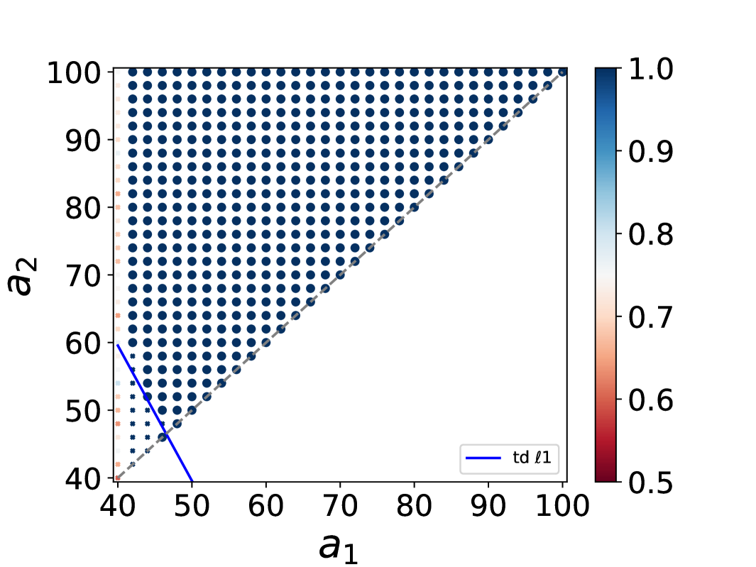
(a) Top-down on level 1

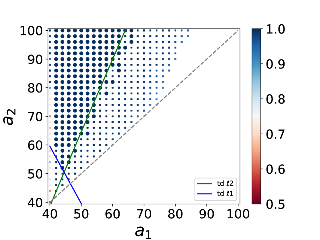
(b) Top-down on level 2

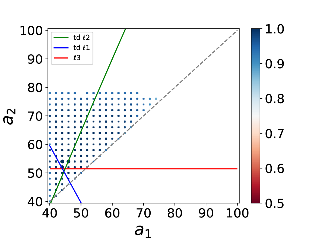
(c) Top-down on level 3

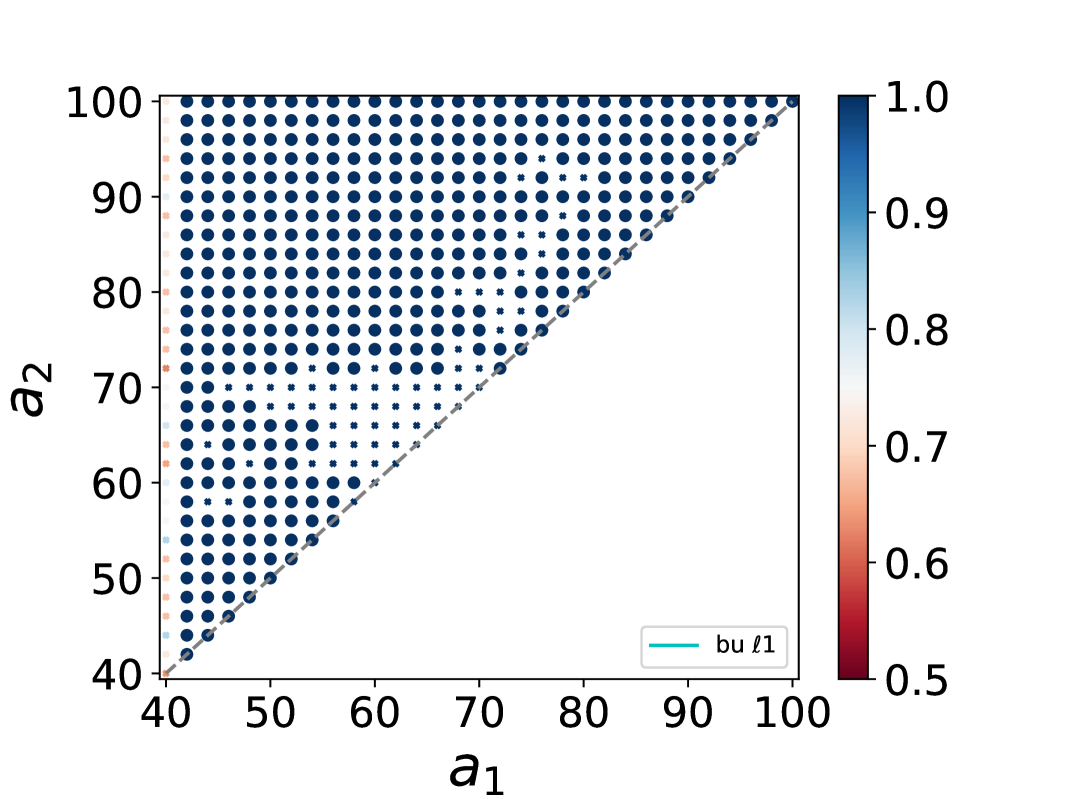
(d) Bottom-up on level 1

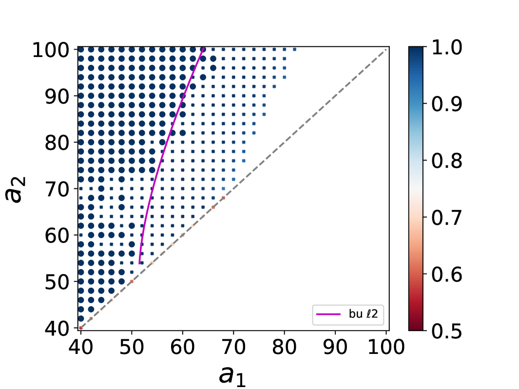
(e) Bottom-up on level 2

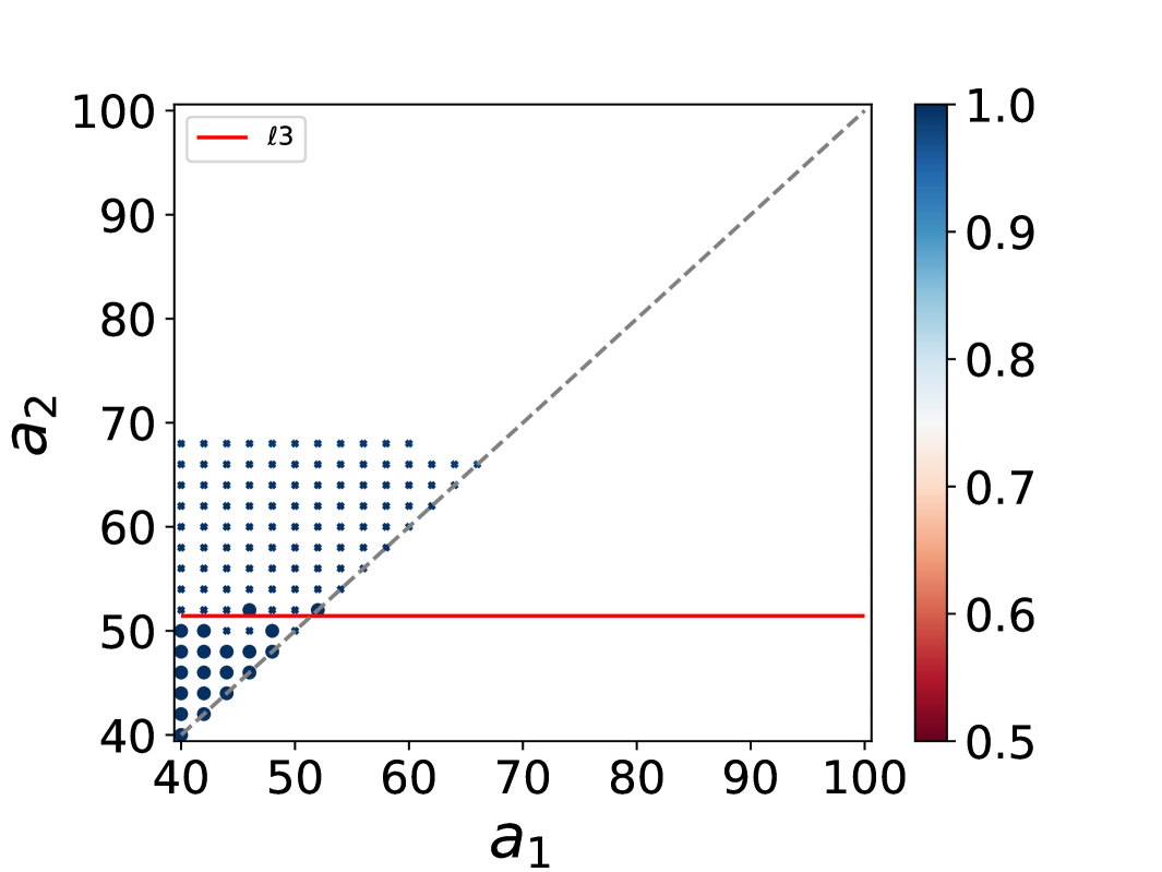
(f) Bottom-up on level 3

Figure 2: Bottom-up and top-down algorithms on BTSBMs with 3 levels, $N=3200$ nodes, and interaction probabilities $p_{k}=a_{k}N^{-1}\log N$, with $a_{0}=40$ and $a_{3}=100$. We vary $a_{1}$ and $a_{2}$ from $a_{0}$ to $a_{3}$. The performance of the algorithms is measured by the accuracy on each level, and the exact recovery threshold on the level is shown in coloured solid lines. Large circles represent exact recovery (i.e., perfect accuracy on each of the 10 runs), while small crosses represent a non-exact recovery (which can still relate to a high accuracy). The theoretical exact recovery thresholds for each algorithm on the various levels are also shown in the figures. For levels 1 and 2, the regimes where exact recovery can be achieved are the areas above the solid line(s). For level 3, the area is limited to below the threshold drawn by the red line (therefore, for top-down the area where exact recovery shall be achieved theoretically is inside the small triangle, which is formed by the 3 lines). The results are averaged over 10 realizations.

6.1.2 Ternary Tree SBMs

As the hierarchical community structure cannot always be represented by a binary tree, we also perform HCD algorithms on ternary tree stochastic block models with 3 levels (the ternary tree is drawn in Figure 3(a)). The model contains 100 nodes in each bottom cluster (thus, in total, there are $N=3^{3}\cdot 100=2700$ nodes). The probability of a link between two nodes whose lowest common ancestor is in level $k$ is given by $p_{k}=a_{k}N^{-1}\log N$.

We first show in Figure 3 the dendrograms and trees obtained by top-down and bottom-up algorithms. Although both algorithms generate binary trees, ternary structures appear in Figures 3(b) and 3(c), as the distances between levels are small. Nevertheless, we observe in Figure 3(c) that the dendrograms obtained by top-down show some inversions.

Next, we proceed as in Section 6.1.1, by fixing $a_{0}$ to 40 and $a_{3}$ to 100, and by varying the values of $a_{1}$ and $a_{2}$ from $a_{0}$ to $a_{3}$ (with the condition $a_{1}<a_{2}$). We observe in Figure 4 profound differences in the performances of top-down and bottom-up. Indeed, in this setting, bottom-up exactly recovers communities up to the theoretical thresholds. Moreover, the accuracy obtained by top-down is lower than the one obtained by bottom-up.

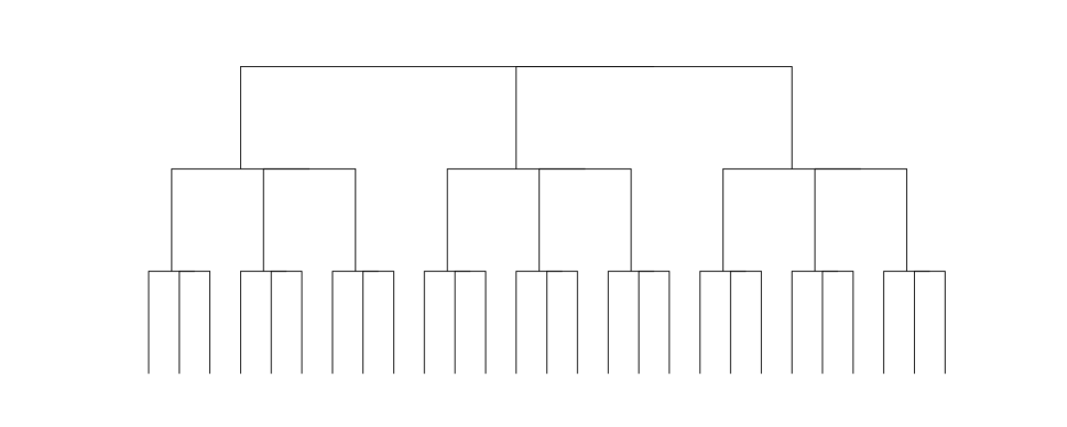
(a) Ground truth tree

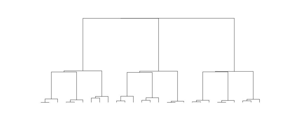
(b) bottom-up

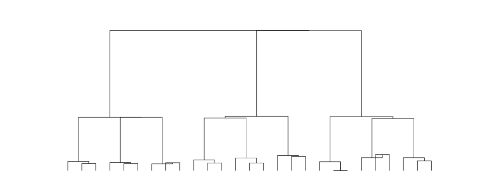
(c) top-down

Figure 3: (a) A ternary tree with 3 levels used as ground truth. (b)-(c) Dendrograms obtained by bottom-up and top-down algorithms on a Ternary Tree Stochastic Block Model with 3 levels, $N=2700$ nodes, and interaction probabilities $p_{k}=a_{k}\frac{\log{N}}{N}$. $(a_{0},a_{1},a_{2},a_{3})=(10,30,40,130)$. The similarity is used to measure the height of the dendrogram. The dendrogram obtained by top-down shows some inversions, which means that the successive splits do not necessarily increase the edge density.

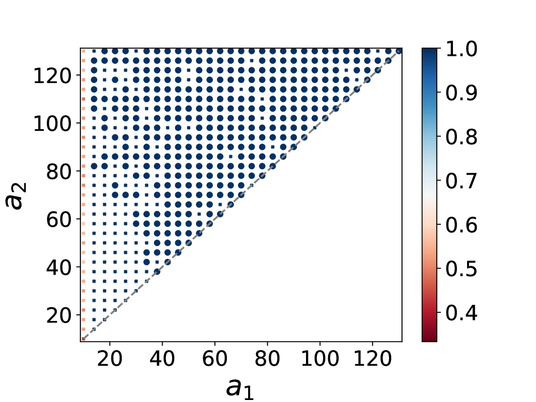
(a) Top-down on level 1

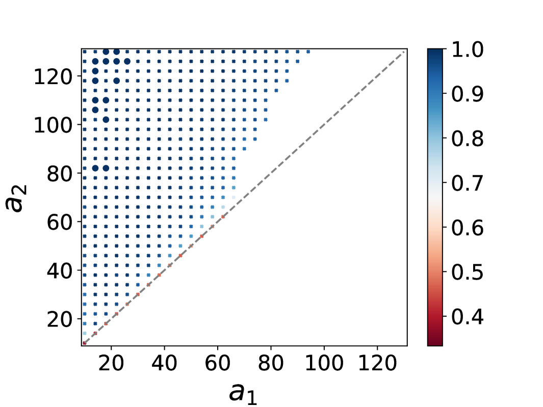
(b) Top-down on level 2

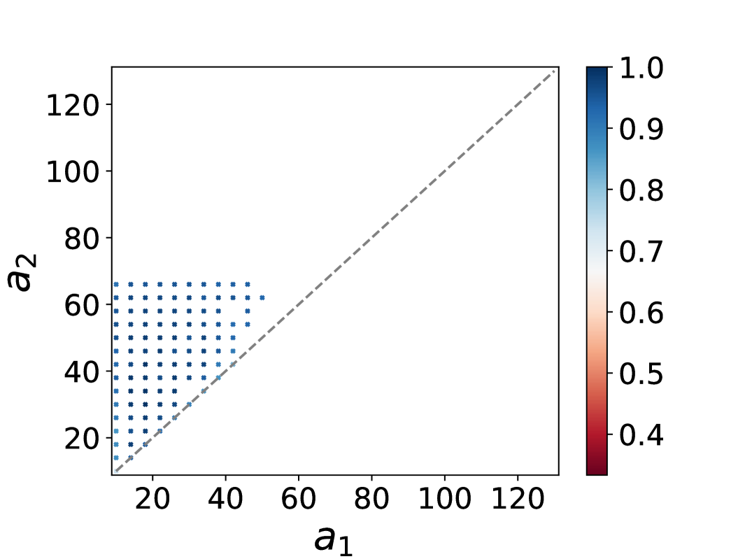
(c) Top-down on level 3

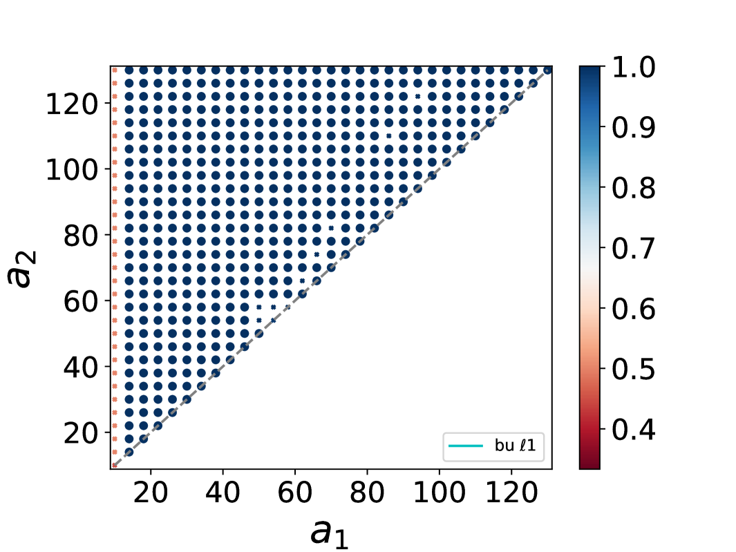
(d) Bottom-up on level 1

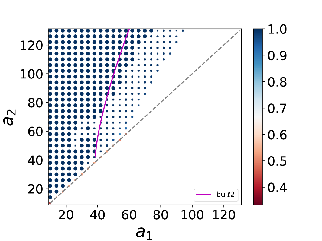
(e) Bottom-up on level 2

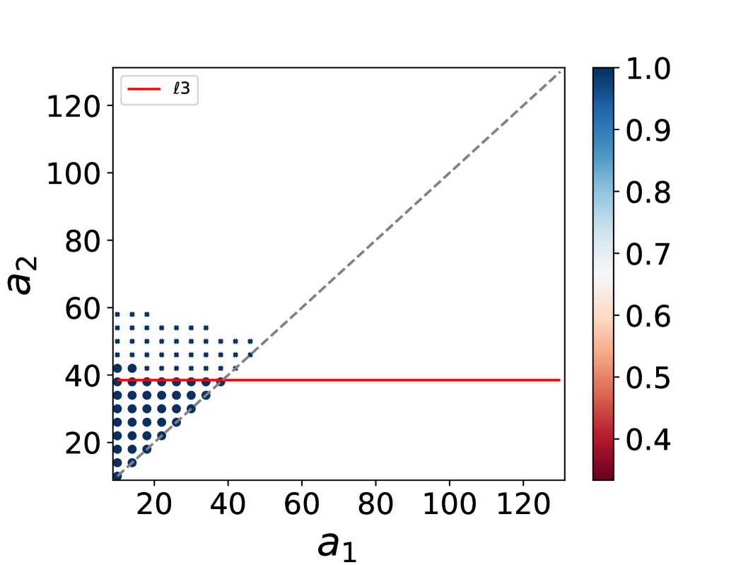
(f) Bottom-up on level 3

Figure 4: Bottom-up and top-down algorithms on ternary BTSBMs with 3 levels, $N=2700$ nodes, and interaction probabilities $p_{k}=a_{k}\frac{\log{N}}{N}$. $a_{0}$ and $a_{3}$ are fixed to 10 and 130, respectively. $a_{1}$ and $a_{2}$ are varied between $a_{0}$ and $a_{3}$. The performance of the algorithms is measured with accuracy on each level, and the exact recovery threshold on the level is shown in coloured solid lines. To emphasize the difference between the exact recovery and others, the exact recovery is shown with large circles, while the non-exact recovery is shown with small crosses. The results are averaged over 10 realizations.

6.1.3 Robustness to outliers

We numerically test the robustness of the bottom-up approach to the errors in the three scenarios discussed in Section 3.3. We denote by $\widehat{\mathcal{T}}^{s}$ the tree obtained by the average-linkage algorithm from the bottom communities $\widehat{\mathcal{C}}^{s}$ (where $\widehat{\mathcal{C}}^{s}$ is defined in Section 3.3). To assess the correct recovery of the tree, we denote by $S\left(\mathcal{T},\mathcal{C}\right)$ the $N$-by-$N$ tree similarity matrix. The elements of this matrix are defined, for $i\in C_{a}$ and $j\in C_{b}$ (with $a,b\in\mathcal{L}_{\mathcal{T}}$), by

$$\Big{(}S\left(\mathcal{T},\mathcal{C}\right)\Big{)}_{ij}\ =\ |\mathrm{lca}_{\mathcal{T}}(a,b)|,$$ (6.1)

where $|\mathrm{lca}_{\mathcal{T}}(a,b)|$ is the depth of the lowest common ancestor of $C_{a}$ and $C_{b}$ in the tree $\mathcal{T}$. The error in recovering the tree is then defined as

$$r_{s}\ =\ \frac{\left\|S\left(\widehat{\mathcal{T}}^{s},\widehat{\mathcal{C}}^{s}\right)-S\left(\mathcal{T},\widehat{\mathcal{C}}^{s}\right)\right\|_{F}^{2}}{\left\|S\left(\mathcal{T},\widehat{\mathcal{C}}^{s}\right)\right\|_{F}^{2}}.$$

This ratio equals $0$ as long as the algorithm succeeds in restoring the tree completely, even if the bottom communities $\widehat{\mathcal{C}}^{s}$ contain mistakes. We plot in Figure 5 the values of these ratios. We show in Figure 5 the recovery success rate $r_{s}$ with varying $\beta$ and noise ratio in the bottom label $\eta$. The results are on the balanced BTSBMs with 3 levels whose edge probability between two nodes whose lowest common ancestor is on level $k$ is defined as $p_{k}=0.08\beta^{3-k}$. The number of nodes in each bottom cluster is $500$ (leading to $N=4000$ nodes in total). As established in Proposition 1, we see that the tree is correctly recovered for scenarios 1 and 2. For scenario 3, the condition $\bar{p}_{1}<p_{d-1}$ might not always be verified, and hence the linkage fails to recover the tree when $\eta$ is too large.

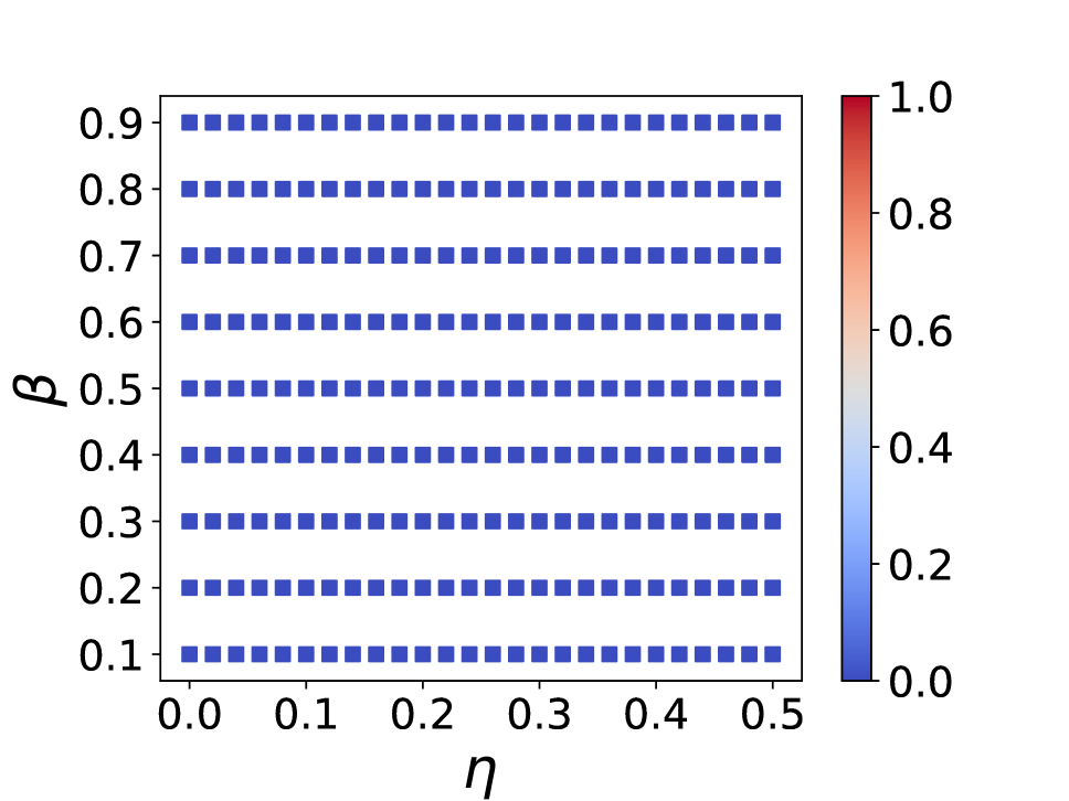
(a) Scenario 1

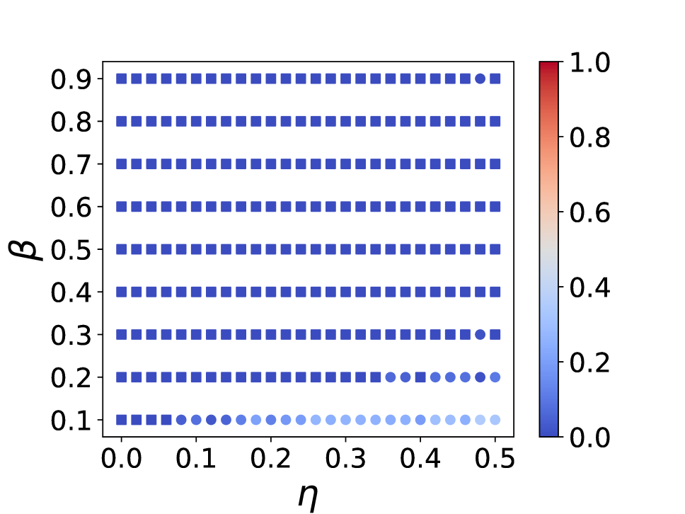
(b) Scenario 2

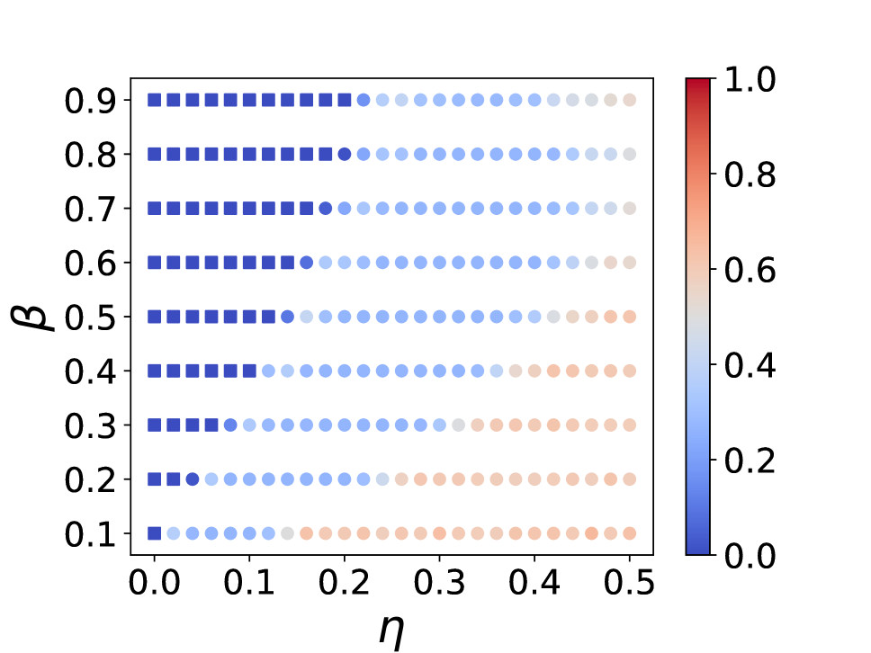
(c) Scenario 3

Figure 5: Recovery from error done by the average-linkage procedure when the initial clustering presents some noise, as discussed in Section 3.3. The results are of the on balanced BTSBMs with 3 levels, $N=4000$, and $p_{k}=0.08\beta^{3-k}$. To emphasize the perfect recovery ($r_{s}=0$), square symbols ($\square$) are used. The values are averaged over 25 realizations.

6.2 Real data sets

6.2.1 High school contact data set

We illustrate the performance of HCD algorithms on a data set of face-to-face contacts between high school students. The data set was collected from the high school Lycée Thiers in Marseilles, France MFB (15) and is available at http://www.sociopatterns.org/. The 9 communities are the classes of the 327 students, and the weighted interactions represent the number of close proximity encounters during 5 school days. We can expect this network to possess hierarchical relationships between communities. Indeed, while each student belongs to one of the 9 classes, these classes also defined the student’s speciality. More precisely, there are four specialisations: ”MP” stands for mathematics and physics, ”PC” for physics and chemistry, ”PSI” for engineering, and ”BIO” for biology. Furthermore, there are three ”MP” classes (MP, MP*1, and MP*2), two ”PC” classes (PC and PC*), one ”PSI” class (PSI*), and three ”BIO” classes (2BIO1, 2BIO2, and 2BIO3). Therefore, we would expect a hierarchical tree to reveal the students’ specialities on a higher level and the students’ classes on a lower level.

The results of the two HCD algorithms are shown in Figure 6. Bottom-up algorithm always detects $31$ communities, while out of 100 runs, top-down algorithm predicts on average 8.93 communities (7 runs detect $8$ communities while the remaining 93 runs detect 9 communities). The predictions of both algorithms are aligned with the ground truth. Indeed, the adjusted mutual information (AMI) VEB (09) between the 9 classes taken as ground truth labels and the predicted communities is $0.938$ for bottom-up and $0.945$ for top-down. We observe that bottom-up successfully recovers the class and specialisation structure, but in addition, finds smaller communities. This likely represents small groups of friends inside a class: the bottom-up algorithm reveals a community structure that is richer than the ground truth itself.

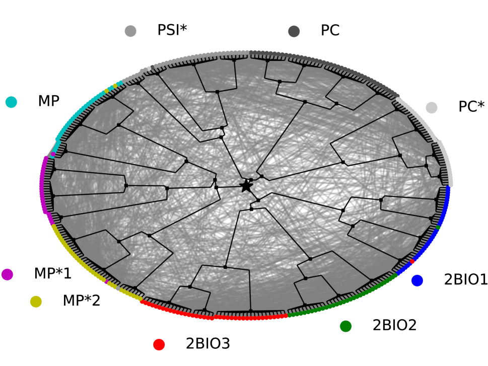
(a) bottom-up

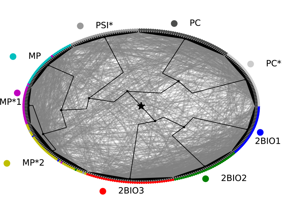
(b) top-down

Figure 6: Output of bottom-up and top-down algorithms on the high school data set. Colours correspond to the true classes, and grey edges indicate contact between the two students. The hierarchical tree is drawn in black, and its root is marked by a star symbol.

6.2.2 Power grid

We next consider the power grid of Continental Europe from the Union for the Coordination of Transmission of Electricity (UCTE) map. We utilize the same data set that has previously been used for HCD SDYB (12). Figures 7 and 8 show the outputs of the bottom-up and top-down, respectively. We observe a higher correlation to geographical positions in the output of the bottom-up. Moreover, the dendrogram obtained by top-down shows a significant amount of inversions.

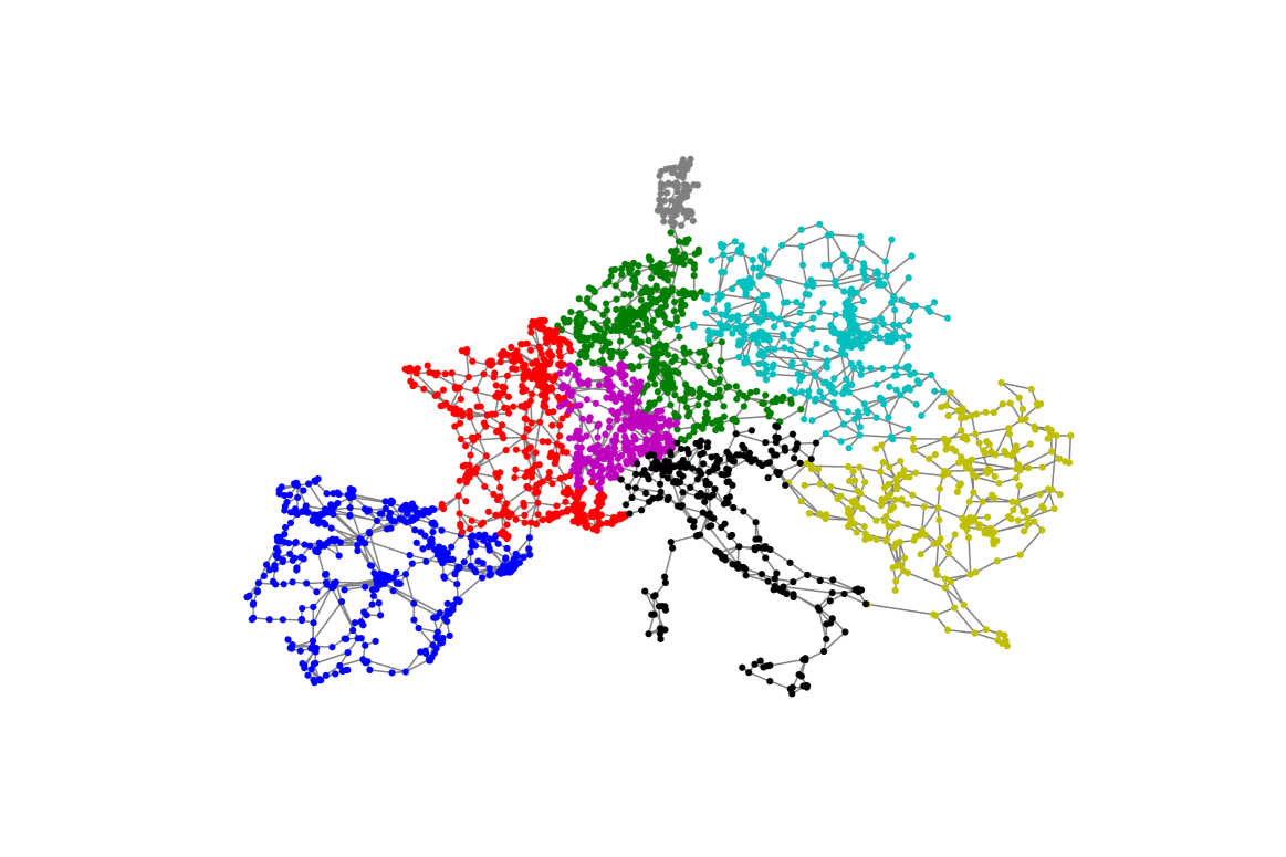
(a) 8 communities.

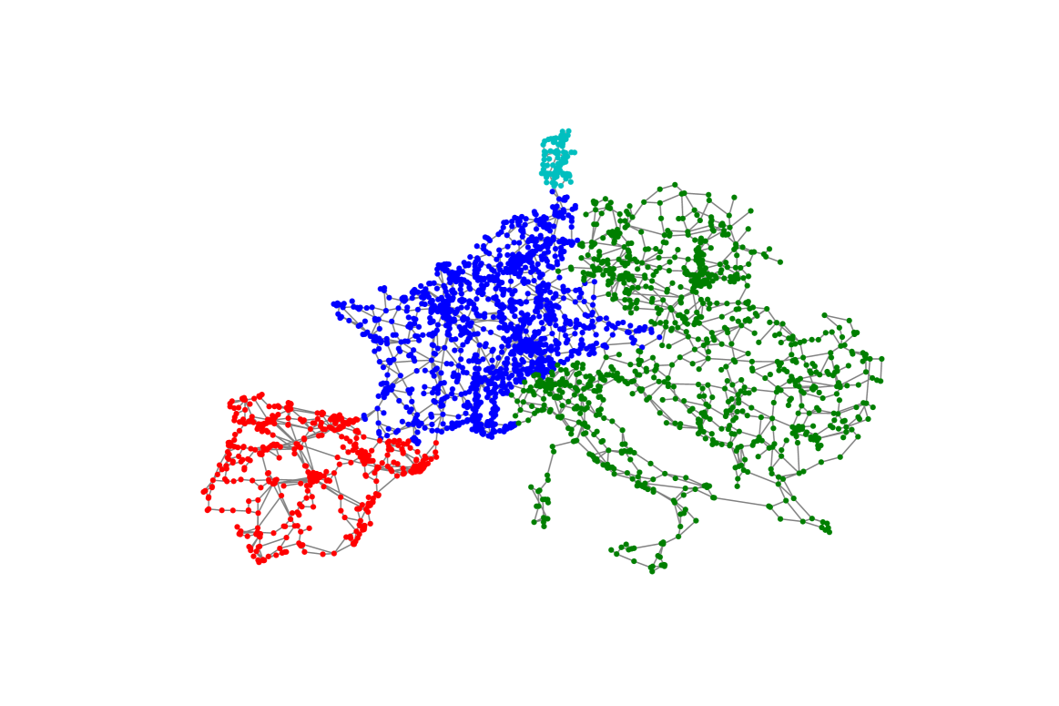
(b) 4 communities.

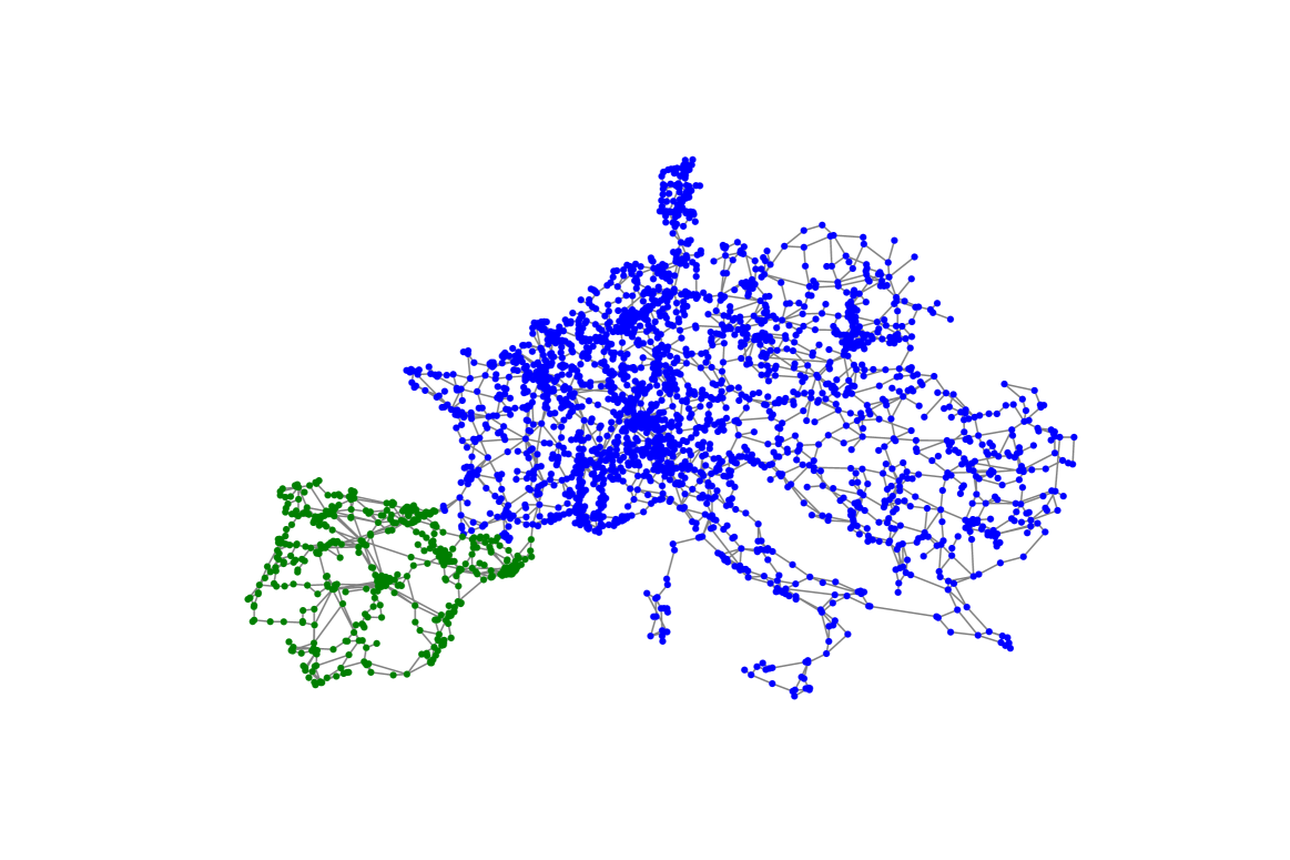
(c) 2 communities.

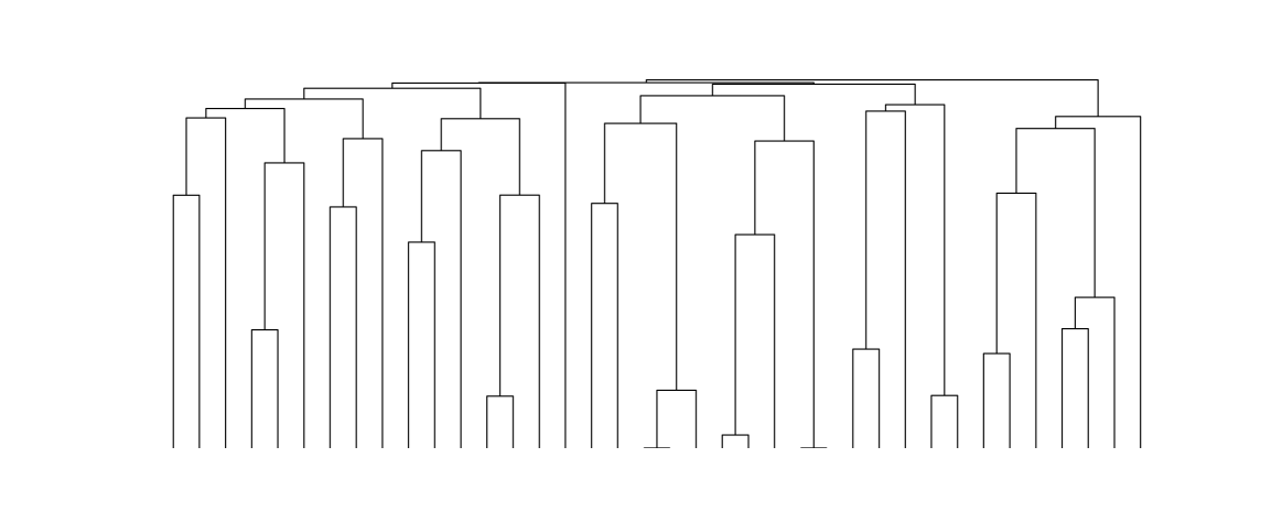
(d) Dendrogram.

Figure 7: Output of bottom-up algorithm on the power grid network.

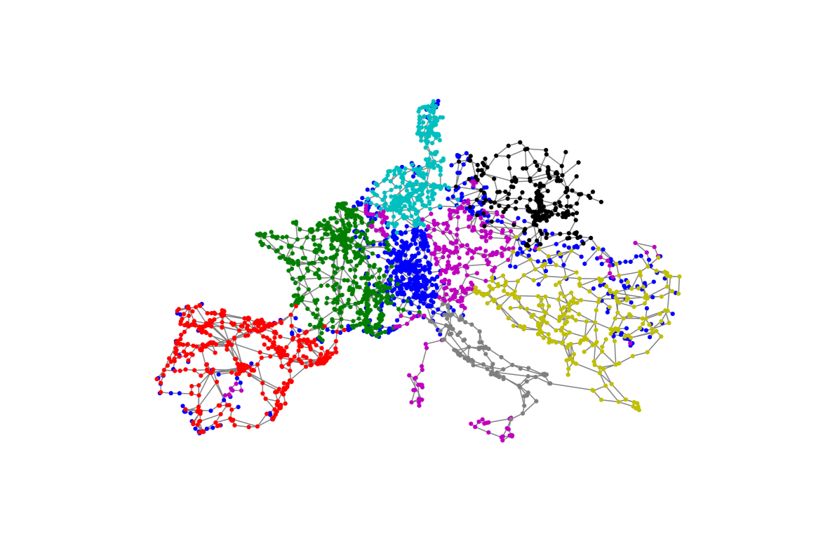
(a) 8 communities.

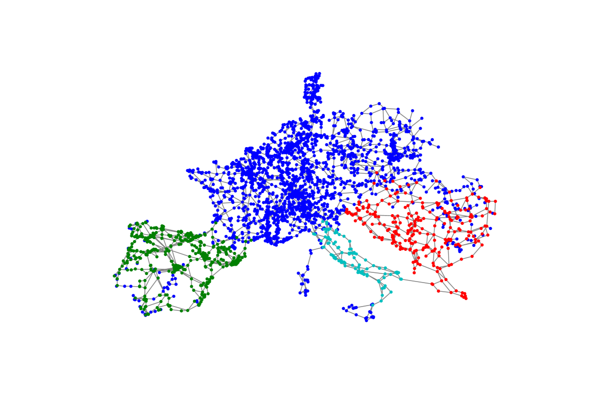
(b) 4 communities.

(c) 2 communities.

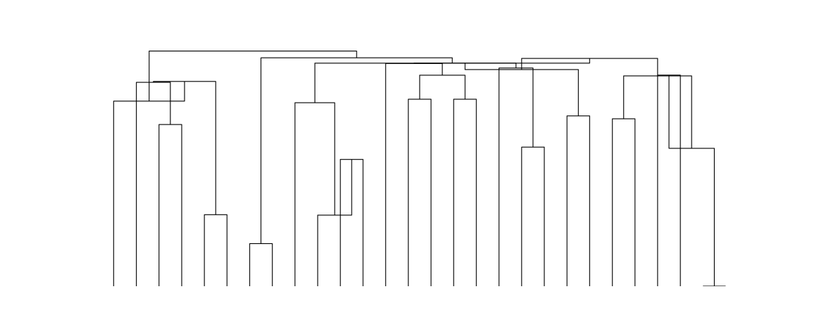
(d) Dendrogram.

Figure 8: Output of recursive spectral bi-partitioning algorithm on the power grid network.

7 Conclusion

Top-down approaches need to make partition decisions for large communities without a way to exploit side information about the internal structure of these communities. As a consequence, such a partition is as difficult as if the communities were flat, and it is challenging to eliminate errors: some nodes can easily be misclassified. These misclassifications are then locked in as the algorithm progresses down to smaller communities. On the other hand, a bottom-up approach inherently exploits lower-level structure, if present. At each level, the algorithm only needs to classify the communities at the next-lower level, rather than classifying all the nodes individually. This is an easier problem (even if some lower-level errors are carried up), because (a) the number of classification decisions is much smaller, and (b) the number of edges available for each individual decision is much larger (number of edges between two lower-level communities versus a number of incident edges on an individual node).

In this paper, we quantify this fundamental advantage within a class of random graph models that generalize the well-studied stochastic block model (SBM) to a hierarchy. We proved that the latent tree of an HSBM can be recovered under weaker conditions than the litterature (average degree scaling as $\omega(1)$). Moreover, we established that super-communities at intermediate levels could be exactly recovered up to the information-theoretic threshold, improving the previously known conditions for top-down algorithms. Finally, we showed that the theoretic advantage of bottom-up carries over to relevant scales and to real-world data: both on synthetic and real data sets that bottom-up HCD typically achieves better performance than top-down HCD.

Appendix A Proofs of Sections 3

A.1 Proof of Theorem 1

Proof of Theorem 1.

We first notice that under the assumptions of Theorem (1), we can almost exactly recover $\mathcal{C}$ (for example by using the clustering algorithms of [4] or of [38]). Let $\widehat{\mathcal{C}}$ be such an estimator.

Next, let $a\neq b\in\mathcal{L}_{\mathcal{T}}$, and recall the definition of the edge density $\rho(\cdot,\cdot)$ in (2.1). Lemma 2 implies that with high probability the edge density between the estimated clusters $\widehat{C}_{a}$ and $\widehat{C}_{b}$ is $\rho(\widehat{C}_{a},\widehat{C}_{b})=(1+o(1))p_{ab}$. Since the network is assortative and the hierarchy is non-flat, this implies that the first step of the linkage finds the two closest clusters, say $\widehat{C}_{a_{1}}$ and $\widehat{C}_{a_{2}}$. Then we see that for $b\in\mathcal{L}_{\mathcal{T}}\backslash\{a_{1},a_{2}\}$ we have $\mathrm{lca}(a_{1},b)=\mathrm{lca}(a_{2},b)$ and hence $p_{a_{1}b}=p_{a_{2}b}$. Therefore, from (2.2),

$$\rho\left(\widehat{C}_{a_{1}\cup a_{2}},\widehat{C}_{b}\right)\ =\ \frac{\left|\widehat{C}_{a_{1}}\right|}{\left|\widehat{C}_{a_{1}}\right|+\left|\widehat{C}_{a_{2}}\right|}\rho\left(\widehat{C}_{a_{1}},\widehat{C}_{b}\right)+\frac{\left|\widehat{C}_{a_{2}}\right|}{\left|\widehat{C}_{a_{1}}\right|+\left|\widehat{C}_{a_{2}}\right|}\rho\left(\widehat{C}_{a_{2}},\widehat{C}_{b}\right)\ =\ (1+o(1))p_{a_{1}b}.$$

So $\rho\left(\widehat{C}_{a_{1}\cup a_{2}},\widehat{C}_{b}\right)=(1+o(1))p_{a_{1}b}$, and repeating this argument, it follows by induction that the average-linkage procedure correctly recovers the tree. ∎

Let us now state and prove the following auxiliary lemma.

Lemma 2.

Consider an HSBM with the same assumptions as in Theorem 1, and let $\widehat{\mathcal{C}}$ be an almost exact estimator of $\mathcal{C}$ (possibly correlated with the graph edges). Then, for any $a,b\in\mathcal{L}_{\mathcal{T}}$ we have $\rho\left(\widehat{C}_{a},\widehat{C}_{b}\right)=(1+o(1))p_{ab}$.

Proof.

Since $\widehat{\mathcal{C}}$ is an almost exact (resp., exact) estimator of $\mathcal{C}$, there exists a permutation $\tau\in\mathcal{S}_{\mathcal{L}_{\mathcal{T}}}$ such that $\sum\limits_{\ell\in\mathcal{L}_{\mathcal{T}}}\left|C_{\ell}\>\Delta\>\widehat{C}_{\tau(\ell)}\right|=o(N)$ (resp., $o(1)$). Without loss of generality, we assume that the permutation $\tau$ in the definition of the loss function (Equation (3.1)) is the identity.

(i) Let us first suppose that $\mathrm{loss}\left(\widehat{\mathcal{C}},\mathcal{C}\right)=o(N)$ and that $p(u)=\Theta(\delta_{N})$. We denote by $Z\in\{0,1\}^{N\times K}$ (resp.$\hat{Z}$) the one-hot representation of the true communities $\mathcal{C}$ (resp. of the predicted communities $\widehat{\mathcal{C}}$), that is $Z_{ic}=1(i\in C_{c})$ and $\hat{Z}_{ic}=1(i\in\widehat{C}_{c})$ for all node $i\in[N]$ and block $c\in\mathcal{L}_{\mathcal{T}}$. Let $a\neq b\in\mathcal{L}_{\mathcal{T}}$. We shorten the edge density $\rho\left(\widehat{C}_{a},\widehat{C}_{b}\right)$ by $\hat{p}_{ab}$. From the definition of the edge density in (2.1), we have

$$\hat{p}_{ab}\ =\ \frac{w\left(\widehat{C}_{a},\widehat{C}_{b}\right)}{\left|\widehat{C}_{a}\right|\cdot\left|\widehat{C}_{b}\right|}\ =\ \frac{\sum_{i\in\widehat{C}_{a},j\in\widehat{C}_{b}}A_{ij}}{\left|\widehat{C}_{a}\right|\cdot\left|\widehat{C}_{b}\right|}\ =\ \frac{\sum_{i<j}\hat{Z}_{ia}\hat{Z}_{jb}A_{ij}}{\sum_{i<j}\hat{Z}_{ia}\hat{Z}_{jb}}.$$

Therefore, a variance-bias decomposition leads to

$$\left|\hat{p}_{ab}-p_{ab}\right| \ \leq\ \underbrace{\left|\frac{\sum_{i<j}\hat{Z}_{ia}\hat{Z}_{jb}\left(A_{ij}-\mathbb{E}A_{ij}\right)}{\sum_{i<j}\hat{Z}_{ia}\hat{Z}_{jb}}\right|}_{E_{1}}+\underbrace{\left|\frac{\sum_{i<j}\hat{Z}_{ia}\hat{Z}_{jb}\mathbb{E}A_{ij}}{\sum_{i<j}\hat{Z}_{ia}\hat{Z}_{jb}}-p_{ab}\right|}_{E_{2}}.$$ (A.1)

Since $\widehat{\mathcal{C}}$ is an almost exact (or even an exact) estimator of $\mathcal{C}$, we have $\sum_{i<j}\hat{Z}_{ia}\hat{Z}_{jb}=(1+o(1))|C_{a}||C_{b}|$. Thus,

$$\sum_{i<j}\hat{Z}_{ia}\hat{Z}_{jb}\ =\ (1+o(1))\pi_{a}\pi_{b}N^{2},$$

using the concentration of multinomial random variables (see for example [2, Lemma A.1]).

Let us bound the two terms $E_{1}$ and $E_{2}$ on the right-hand side of (A.1) separately. To handle the first term, let us first notice that $9N^{-1}\leq 2N^{-1}(N-1)^{-1}\sum_{i<j}\operatorname{Var}(A_{ij})\leq p_{\max}$ where $p_{\max}=\max\limits_{a,b}p_{ab}$. Thus, [19, Lemma 4.1] ensures that with probability at least $1-e^{3}5^{-N}$ we have

$$\sup_{s,t\in\{-1,1\}^{n}}\left|\sum_{i,j}\left(A_{ij}-\mathbb{E}A_{ij}\right)s_{i}t_{j}\right|\ \leq\ 3N\sqrt{Np_{\max}}.$$

Applying Grothendieck’s inequality [19, Theorem 3.1], we obtain

$$\sup_{\begin{subarray}{c}X_{1},\cdots,X_{N}\\ \forall i\in[N]\colon\|X_{i}\|_{2}\leq 1\end{subarray}}\left|\sum_{i<j}\left(A_{ij}-\mathbb{E}A_{ij}\right)X_{i}^{T}X_{j}\right|\ \leq\ 3cN\sqrt{Np_{\max}},$$

where $c$ is Grothendieck’s constant, verifying $0<c<2$. Hence, w.h.p.,

$$E_{1}\ =\ O\left(\sqrt{\frac{p_{\max}}{n}}\right)\ =\ o(\delta_{N}).$$

To handle the second term $E_{2}$ in the right-hand side of (A.1), we first notice that

$$E_{2} \ =\ \frac{\left|\sum\limits_{i<j}\hat{Z}_{ia}\hat{Z}_{jb}\left(\mathbb{E}A_{ij}-p_{ab}\right)\right|}{\sum\limits_{i<j}\hat{Z}_{ia}\hat{Z}_{jb}}.$$ (A.2)

Moreover, for all $i,j\in[N]$ we have

$$\mathbb{E}A_{ij}=\sum_{a^{\prime},b^{\prime}\in\mathcal{L}_{\mathcal{T}}}p_{a^{\prime}b^{\prime}}Z_{ia^{\prime}}Z_{jb^{\prime}},$$

since if $\mathbb{E}A_{ij}=p_{a^{\prime}b^{\prime}}$ if $i\in C_{a^{\prime}}$ and $j\in C_{b^{\prime}}$. Thus,

$$\mathbb{E}A_{ij}-p_{ab}\ =\ \sum_{\begin{subarray}{c}a^{\prime},b^{\prime}\in\mathcal{L}_{\mathcal{T}}\\ (a^{\prime},b^{\prime})\neq(a,b)\end{subarray}}(p_{a^{\prime}b^{\prime}}-p_{ab})Z_{ia^{\prime}}Z_{jb^{\prime}}.$$

Let $c=\max_{a^{\prime},b^{\prime}}\frac{p_{a^{\prime}b^{\prime}}}{p_{ab}}$. Under our assumptions, $c=\Theta(1)$. We bound the numerator appearing in Equation (A.2) as follows:

$$\left|\sum\limits_{i<j}\hat{Z}_{ia}\hat{Z}_{jb}\left(\mathbb{E}A_{ij}-p_{ab}\right)\right| \ \leq\ p_{ab}\left(c+1\right)\sum_{\begin{subarray}{c}a^{\prime},b^{\prime}\in\mathcal{L}_{\mathcal{T}}\\ (a^{\prime},b^{\prime})\neq(a,b)\end{subarray}}\sum_{i<j}\hat{Z}_{ia}\hat{Z}_{jb}Z_{ia^{\prime}}Z_{jb^{\prime}}$$

$$\ \leq\ 2cp_{ab}\sum_{\begin{subarray}{c}a^{\prime},b^{\prime}\in\mathcal{L}_{\mathcal{T}}\\ (a^{\prime},b^{\prime})\neq(a,b)\end{subarray}}\left|\widehat{C}_{a}\cap C_{a^{\prime}}\right|\cdot\left|\widehat{C}_{b}\cap C_{b^{\prime}}\right|,$$

since $c\geq 1$. Let us denote $V\backslash C_{a}=\cup_{a^{\prime}\neq a}C_{a^{\prime}}$ by $C_{a}^{c}$. We have

$$\sum_{\begin{subarray}{c}a^{\prime},b^{\prime}\in\mathcal{L}_{\mathcal{T}}\\ (a^{\prime},b^{\prime})\neq(a,b)\end{subarray}}\left|\widehat{C}_{a}\cap C_{a^{\prime}}\right|\cdot\left|\widehat{C}_{b}\cap C_{b^{\prime}}\right| \ =\ \sum_{a^{\prime}\neq a}\sum_{b^{\prime}\in\mathcal{L}_{\mathcal{T}}}\left|\widehat{C}_{a}\cap C_{a^{\prime}}\right|\cdot\left|\widehat{C}_{b}\cap C_{b^{\prime}}\right|+\left|\widehat{C}_{a}\cap C_{a}\right|\sum_{b^{\prime}\neq b}\left|\widehat{C}_{b}\cap C_{b^{\prime}}\right|$$

$$\ =\ \left|\widehat{C}_{a}\cap C^{c}_{a}\right|\cdot\left|\widehat{C}_{b}\right|+\left|\widehat{C}_{a}\cap C_{a}\right|\cdot\left|\widehat{C}_{b}\cap C_{b}^{c}\right|$$

$$\ \leq\ \left(\left|\widehat{C}_{b}\right|+\left|\widehat{C}_{a}\right|\right)\mathrm{loss}\left(\mathcal{C},\widehat{\mathcal{C}}\right),$$

where in the last line we used $\mathrm{loss}\left(\mathcal{C},\widehat{\mathcal{C}}\right)=\sum_{a\in\mathcal{L}_{\mathcal{T}}}=\left|\widehat{C}_{a}\cap C^{c}_{a}\right|$. Hence,

$$E_{2}\ \leq\ 2cp_{ab}\frac{\left|\widehat{C}_{b}\right|+\left|\widehat{C}_{a}\right|}{\left|\widehat{C}_{a}\right|\cdot\left|\widehat{C}_{b}\right|}\mathrm{loss}\left(\mathcal{C},\widehat{\mathcal{C}}\right),$$

and this indeed ensures that $E_{2}=o(p_{ab})$. ∎

A.2 Proof of Proposition 1

Before proving Proposition 1, let us recall the following version of the Chernoff bounds.

Lemma 3 (Chernoff bounds for binomial distribution).

Let $X\sim\operatorname{Bin}(n,p)$ be a binomial distribution such that $\mathbb{E}X=np\gg 1$. Then we have with high probability

$$X\ =\ (1+o(1))\mathbb{E}X.$$

We can now prove Proposition 1.

Proof of Proposition 1.

We proceed by showing that for each scenario $s\in\{1,2,3\}$ the edge density $\rho\left(\tilde{C}_{a}^{s},\tilde{C}_{b}^{s}\right)$ is concentrated around its mean. We denote $O_{ab}^{s}=C_{a}\cap\tilde{C}_{b}^{s}$ the nodes in cluster $C_{a}$ but assigned to cluster $\tilde{C}_{b}^{s}$. In particular, the set of all misclassified nodes $O^{s}$ is given by $O^{s}=\cup_{\begin{subarray}{c}a,b\in\mathcal{L}_{\mathcal{T}}\\ b\neq a\end{subarray}}O_{ab}^{s}$ and is independent of the edges. Therefore, $w\left(O_{ab}^{s},O_{cd}^{s}\right)\sim\operatorname{Bin}\left(|O_{ab}^{s}|\cdot|O_{cd}^{s}|,p_{ac}\right)$. We notice, from the definition of the edge density (2.1) and the fact that $\tilde{C}^{s}_{a}=\cup_{k\in\mathcal{L}_{\mathcal{T}}}O_{ka}^{s}$, that

$$\rho\left(\tilde{C}_{a}^{s},\tilde{C}_{b}^{s}\right)\ =\ \frac{w\left(\tilde{C}_{a}^{s},\tilde{C}_{b}^{s}\right)}{\left|\tilde{C}_{a}^{s}\right|\cdot\left|\tilde{C}_{b}^{s}\right|}\quad\text{ with }\quad w\left(\tilde{C}_{a}^{s},\tilde{C}_{b}^{s}\right)\ =\ \sum_{k,\ell\in\mathcal{L}_{\mathcal{T}}}w\left(O_{ka}^{s},O_{\ell b}^{s}\right),$$ (A.3)

We will express $\mathbb{E}w\left(O_{ka}^{s},O_{\ell b}^{s}\right)$ for each scenario. The concentration $\rho\left(\tilde{C}_{a}^{s},\tilde{C}_{b}^{s}\right)$ around its mean then follows from Chernoff’s bounds.

In the following of the proof, we let $a,b,c\in\mathcal{L}_{\mathcal{T}}$ be three different leaves such that $b$ is the closest leaf from $a$, i.e., $b=\operatorname*{arg\,max}\limits_{k\in\mathcal{L}_{\mathcal{T}}}|\mathrm{lca}(a,k)|$ and $c\not\in\{a,b\}$. To conclude that the linkage procedure outputs the correct tree, we have to verify that

$$\forall c\not\in\{a,b\}\colon\rho\left(\tilde{C}_{a}^{s},\tilde{C}_{b}^{s}\right)>\rho\left(\tilde{C}_{a}^{s},\tilde{C}_{c}^{s}\right).$$

We will show this separately for each three scenarios.

(i) Scenario 1: Since $\tilde{C}_{a}^{1}\cap O^{1}\subset C_{b}$ and $\tilde{C}_{b}\cap O^{1}\subset C_{a}$, it comes

$$w\left(\tilde{C}_{a}^{1},\tilde{C}_{b}^{1}\right) \ =\ w\left(O_{aa}^{1},O_{bb}^{1}\right)+w\left(O_{aa}^{1},O_{ab}^{1}\right)+w\left(O_{ba}^{1},O_{bb}^{1}\right)+w\left(O_{ba}^{1},O_{ab}^{1}\right).$$

(We used (A.3) and the fact that for scenario 1 we have $O_{ka}^{s}=\emptyset$ if $k\neq\{a,b\}$). Using $\mathbb{E}\left|O_{aa}^{1}\right|=\mathbb{E}\left|O_{bb}^{1}\right|=(1-\eta)\frac{N}{K}$, $\mathbb{E}\left|O_{ab}^{1}\right|=\mathbb{E}\left|O_{ba}^{1}\right|=\eta\frac{N}{K}$ together with Lemma 3, it comes

$$w\left(\tilde{C}_{a}^{1},\tilde{C}_{b}^{1}\right)\ =\ (1+o(1))\left(\frac{N}{K}\right)^{2}\left(\left((1-\eta)^{2}+\eta^{2}\right)p_{ab}+\eta(1-\eta)(p_{aa}+p_{bb})\right)$$

and thus

$$\rho\left(\tilde{C}_{a}^{1},\tilde{C}_{b}^{1}\right)\ =\ (1+o(1))\left(\left((1-\eta)^{2}+\eta^{2}\right)p_{ab}+\eta(1-\eta)(p_{aa}+p_{bb})\right)$$

where we used $\left|\tilde{C}_{a}^{s}\right|=(1+o(1))\frac{N}{K}$ whp (via Chernoff bounds).

By proceeding similarly, denoting $k$ the nearest leaf from a leaf $c\in\mathcal{L}_{\mathcal{T}}\backslash\{a,b\}$ and noticing that $p_{ac}=p_{bk}=p_{bc}=p_{bk}$, we have

$$w\left(\tilde{C}_{a}^{1},\tilde{C}_{c}^{1}\right) \ =\ w\left(O_{aa}^{1},O_{cc}^{1}\right)+w\left(O_{aa}^{1},O_{kc}^{1}\right)+w\left(O_{ba}^{1},O_{cc}^{1}\right)+w\left(O_{ba}^{1},O_{kc}^{1}\right)$$

$$\ =\ (1+o(1))\left(\frac{N}{K}\right)^{2}\left((1-\eta)^{2}p_{ac}+\eta(1-\eta)(p_{ak}+p_{bc})+\eta^{2}p_{bk}\right)$$

$$\ =\ (1+o(1))\left(\frac{N}{K}\right)^{2}p_{ac}.$$

Therefore,

$$\rho\left(\tilde{C}_{a}^{1},\tilde{C}_{c}^{1}\right)\ =\ (1+o(1))p_{ac}.$$

Finally, assortativity implies $\min(p_{aa},p_{bb})>p_{ab}>p_{ac}$, and thus $\rho\left(\tilde{C}_{a}^{1},\tilde{C}_{b}^{1}\right)>\rho\left(\tilde{C}_{a}^{1},\tilde{C}_{c}^{1}\right)$ for any $c\not\in\{a,b\}$. Therefore $\widehat{\mathcal{T}}^{1}=\mathcal{T}$.

(ii) Scenario 2: the random variables $w\left(O_{ka}^{2},O_{\ell b}^{2}\right)$ are binomially distributed such that

$$\mathbb{E}w\left(O_{ka}^{2},O_{\ell b}^{2}\right)\ =\ \left(\frac{N}{K}\right)^{2}\times\begin{cases}\left(1-\eta+\frac{\eta}{K}\right)^{2}p_{ab}&\text{ if }(k,\ell)=(a,b),\\ \left(1-\eta+\frac{\eta}{K}\right)\frac{\eta}{K}p_{a\ell}&\text{ if }k=a\text{ and }\ell\neq b,\\ \left(1-\eta+\frac{\eta}{K}\right)\frac{\eta}{K}p_{kb}&\text{ if }k\neq a\text{ and }\ell=b,\\ \left(\frac{\eta}{K}\right)^{2}p_{k\ell}&\text{ if }k\neq a\text{ and }\ell\neq b.\\ \end{cases}$$

Noticing that $p_{ak}=p_{kb}$ when $k\not\in\{a,b\}$ and that $p_{aa}=p_{bb}$, we have

$$\mathbb{E}w\left(\tilde{C}_{a}^{2},\tilde{C}_{b}^{2}\right) \ =\ \left(\frac{N}{K}\right)^{2}\left(\left(1-\eta+\frac{\eta}{K}\right)^{2}p_{ab}+\left(1-\eta+\frac{\eta}{K}\right)\frac{\eta}{K}\left(\sum_{\ell\neq b}p_{a\ell}+\sum_{k\neq a}p_{bk}\right)+\left(\frac{\eta}{K}\right)^{2}\sum_{k\neq a}\sum_{\ell\neq b}p_{k\ell}\right)$$

$$\ =\ \left(\frac{N}{K}\right)^{2}\left(\left(1-\eta+\frac{\eta}{K}\right)^{2}p_{ab}+2\left(1-\eta+\frac{\eta}{K}\right)\frac{\eta}{K}\sum_{k\neq a}p_{bk}+\left(\frac{\eta}{K}\right)^{2}\sum_{k\neq a}\sum_{\ell\neq b}p_{k\ell}\right).$$

The quantity $\sum\limits_{k\in\mathcal{L}_{\mathcal{T}}}p_{bk}$ does not depend on $b$, and we denote by $S$ its value. In particular,

$$\sum_{k\neq a}p_{bk} \ =\ S-p_{ab},$$

$$\sum_{k\neq a}\sum_{\ell\neq b}p_{k\ell} \ =\ \sum_{k\neq a}S-\sum_{k\neq a}p_{kb}\ =\ (|\mathcal{T}|-2)S+p_{ab},$$

where $|\mathcal{T}|$ denotes the number of nodes of $\mathcal{T}$. Therefore, we have whp

$$\rho\left(\tilde{C}_{a}^{2},\tilde{C}_{b}^{2}\right)\ =\ (1+o(1))\left(\left(1-\eta+\frac{\eta}{K}\right)^{2}p_{ab}+2\left(1-\eta+\frac{\eta}{K}\right)\frac{\eta}{K}\left(S-p_{ab}\right)+\left(\frac{\eta}{K}\right)^{2}\left((|\mathcal{T}|-2)S+p_{ab}\right)\right).$$

By proceeding similarly, we obtain whp that for any $c\neq b$,

$$\rho\left(\tilde{C}_{a}^{2},\tilde{C}_{c}^{2}\right) \ =\ (1+o(1))\left(\left(1-\eta+\frac{\eta}{K}\right)^{2}p_{ac}+\left(1-\eta+\frac{\eta}{K}\right)\frac{\eta}{K}\left(\sum_{\ell\neq c}p_{a\ell}+\sum_{k\neq a}p_{kc}\right)+\left(\frac{\eta}{K}\right)^{2}\sum_{k\neq a}\sum_{\ell\neq c}p_{k\ell}\right)$$

$$\ =\ (1+o(1))\left(\left(1-\eta+\frac{\eta}{K}\right)^{2}p_{ac}+2\left(1-\eta+\frac{\eta}{K}\right)\frac{\eta}{K}\left(S-p_{ac}\right)+\left(\frac{\eta}{K}\right)^{2}\left((|\mathcal{T}|-2)S+p_{ac}\right)\right).$$

Finally,

$$\rho\left(\tilde{C}_{a}^{2},\tilde{C}_{b}^{2}\right)-\rho\left(\tilde{C}_{a}^{2},\tilde{C}_{c}^{2}\right)\ =\ (1+o(1))\Bigg{(}\left(1-\eta+\frac{\eta}{K}\right)^{2}\left(p_{ab}-p_{ac}\right)+2\left(1-\eta+\frac{\eta}{K}\right)\frac{\eta}{K}\left(p_{ac}-p_{ab}\right)$$

$$\qquad\quad\qquad\quad\qquad+\left(\frac{\eta}{K}\right)^{2}(p_{ab}-p_{ac})\Bigg{)}$$

$$\ =\ (1+o(1))(p_{ab}-p_{ac})\left(1-\eta\right)^{2}>0,$$

and hence the linkage algorithm merges the communities in the correct order.

(iii) Scenario 3: we say a tree node $t\in\mathcal{T}$ is in the super-community $0$ if the first digit of its binary string representation is $0$ and is in block one otherwise, and we denote by $B_{0}$ and $B_{1}$ the sets of nodes in super-community $0$ and $1$, respectively. Without loss of generalities, we assume that $a\in B_{0}$ (and hence $b\in B_{0}$ as well). We have for all $k,\ell\in\mathcal{L}_{\mathcal{T}}$

$$\mathbb{E}w\left(O_{ka}^{3},O_{\ell b}^{3}\right)\ =\ \left(\frac{N}{K}\right)^{2}\times\begin{cases}(1-\eta)^{2}p_{d-1}&\text{ if }(k,\ell)=(a,b),\\ (1-\eta)\frac{\eta}{|B_{1}|}p_{0}&\text{ if }k=a\text{ and }\ell\in B_{1},\\ (1-\eta)\frac{\eta}{|B_{1}|}p_{0}&\text{ if }k\in B_{1}\text{ and }\ell=b,\\ \left(\frac{\eta}{|B_{1}|}\right)^{2}p_{k\ell}&\text{ if }k\in B_{1}\text{ and }\ell\in B_{1},\\ 0&\text{ otherwise.}\end{cases}$$

Using that $|B_{1}|=K/2$, we have whp

$$\rho\left(\tilde{C}^{3}_{a},\tilde{C}^{3}_{b}\right) \ =\ (1+o(1))\left((1-\eta)^{2}p_{d-1}+(1-\eta)\frac{\eta}{K/2}\left(\sum_{\ell\in B_{1}}p_{0}+\sum_{k\in B_{1}}p_{0}\right)+\left(\frac{\eta}{K/2}\right)^{2}\sum_{k\in B_{1}}\sum_{\ell\in B_{1}}p_{k\ell}\right).$$

We notice that the quantity $\frac{1}{|B_{1}|}\sum_{\ell\in B_{1}}p_{k\ell}$ is independent of $k$ and is the expected edge density in the super-community at level 1 (i.e., the super-community $\cup_{k\in B_{1}}C_{k}$). Let us denote by $\bar{p}_{1}$ its value. We have $\bar{p}_{1}=\frac{1}{2^{d-1}}\left(p_{d}+\sum_{k=1}^{d-1}2^{k-1}p_{d-k}\right)$, and

$$\rho\left(\tilde{C}^{3}_{a},\tilde{C}^{3}_{b}\right) \ =\ (1+o(1))\left((1-\eta)^{2}p_{d-1}+2(1-\eta)\eta p_{0}+\eta^{2}\bar{p}_{1}\right).$$

Similarly, let $c\in B_{0}\backslash\{a,b\}$. We have whp

$$\rho\left(\tilde{C}^{3}_{a},\tilde{C}^{3}_{c}\right)\ =\ (1+o(1))\left((1-\eta)^{2}p_{ac}+2\eta(1-\eta)p_{0}+\eta^{2}\bar{p}_{1}\right),$$

and therefore the network assortativity implies $\rho\left(\tilde{C}^{3}_{a},\tilde{C}^{3}_{b}\right)>\rho\left(\tilde{C}^{3}_{a},\tilde{C}^{3}_{c}\right)$ for all $c\in B_{0}\backslash\{a,b\}$.

Finally, let $c\in B_{1}$. We have

$$\mathbb{E}w\left(O_{ka}^{3},O_{\ell c}^{3}\right)\ =\ \left(\frac{N}{K}\right)^{2}\times\begin{cases}(1-\eta)^{2}p_{0}&\text{ if }(k,\ell)=(a,c),\\ (1-\eta)\frac{\eta}{|B_{0}|}p_{a\ell}&\text{ if }k=a\text{ and }\ell\in B_{0},\\ (1-\eta)\frac{\eta}{|B_{1}|}p_{kc}&\text{ if }k\in B_{1}\text{ and }\ell=c,\\ \eta^{2}p_{0}&\text{ if }k\in B_{1}\text{ and }\ell\in B_{0},\\ 0&\text{ otherwise.}\end{cases}$$

Thus,

$$\rho\left(\tilde{C}^{3}_{a},\tilde{C}^{3}_{c}\right) \ =\ (1+o(1))\left(\left((1-\eta)^{2}+\eta^{2}\right)p_{0}+(1-\eta)\frac{\eta}{K/2}\left(\sum_{\ell\in B_{0}}p_{a\ell}+\sum_{k\in B_{1}}p_{kc}\right)\right).$$

We notice that $\frac{1}{K/2}\sum_{\ell\in B_{0}}p_{a\ell}=\frac{1}{K/2}\sum_{k\in B_{1}}p_{kc}=\bar{p}_{1}$. Hence

$$\rho\left(\tilde{C}^{3}_{a},\tilde{C}^{3}_{c}\right) \ =\ (1+o(1))\left(\left((1-\eta)^{2}+\eta^{2}\right)p_{0}+2\eta(1-\eta)\bar{p}_{1}\right).$$

In particular, we notice that

$$\rho\left(\tilde{C}^{3}_{a},\tilde{C}^{3}_{b}\right)-\rho\left(\tilde{C}^{3}_{a},\tilde{C}^{3}_{c}\right) \ =\ (1+o(1))\left((1-\eta)^{2}(p_{d-1}-p_{0})+(\eta^{2}-2\eta(1-\eta))(\bar{p}_{1}-p_{0})\right).$$ (A.4)

If $p_{d-1}>\bar{p}_{1}$ we have

$$\rho\left(\tilde{C}^{3}_{a},\tilde{C}^{3}_{b}\right)-\rho\left(\tilde{C}^{3}_{a},\tilde{C}^{3}_{c}\right) >(1+o(1))(\bar{p}_{1}-p_{0})\left(1-2\eta\right)^{2},$$

and this quantity is positive since $\bar{p}_{1}>p_{0}$. Therefore, $p_{d-1}>\bar{p}_{1}$ is one sufficient condition to recover the tree, and this proves point (3a) of Proposition 1.

Finally, when $p_{d-1}\leq\bar{p}_{1}$, we return to Equation (A.4) and we have (by ”completing the square”)

$$\rho\left(\tilde{C}^{3}_{a},\tilde{C}^{3}_{b}\right)-\rho\left(\tilde{C}^{3}_{a},\tilde{C}^{3}_{c}\right)\ =\ (1+o(1))\left((p_{d-1}+3\bar{p}_{1}-4p_{0})\eta^{2}-2(p_{d-1}+\bar{p}_{1}-2p_{0})\eta+(p_{d-1}-p_{0})\right)$$

$$\ =\ (1+o(1))\Bigg{(}(p_{d-1}+3\bar{p}_{1}-4p_{0})\left(\eta-\frac{p_{d-1}+\bar{p}_{1}-2p_{0}}{p_{d-1}+3\bar{p}_{1}-4p_{0}}\right)^{2}+(p_{d-1}-p_{0})$$

$$\qquad\quad\qquad\quad\qquad-\frac{(p_{d-1}+\bar{p}_{1}-2p_{0})^{2}}{p_{d-1}+3\bar{p}_{1}-4p_{0}}\Bigg{)}$$

$$\ =\ (1+o(1))\left((p_{d-1}+3\bar{p}_{1}-4p_{0})\left(\eta-\frac{p_{d-1}+\bar{p}_{1}-2p_{0}}{p_{d-1}+3\bar{p}_{1}-4p_{0}}\right)^{2}-\frac{(\bar{p}_{1}-p_{d-1})(\bar{p}_{1}-p_{0})}{p_{d-1}+3\bar{p}_{1}-4p_{0}}\right).$$

Because $(p_{d-1}+3\bar{p}_{1}-4p_{0})>0$, this quantity is positive if $\eta<\eta_{-}$ or if $\eta>\eta_{+}$, where

$$\eta_{-} \ =\ \frac{p_{d-1}+\bar{p}_{1}-2p_{0}-\sqrt{(\bar{p}_{1}-p_{d-1})(\bar{p}_{1}-p_{0})}}{p_{d-1}+3\bar{p}_{1}-4p_{0}},$$

$$\eta_{+} \ =\ \frac{p_{d-1}+\bar{p}_{1}-2p_{0}+\sqrt{(\bar{p}_{1}-p_{d-1})(\bar{p}_{1}-p_{0})}}{p_{d-1}+3\bar{p}_{1}-4p_{0}}.$$

We notice that $\eta_{+}=\frac{\sqrt{\bar{p}_{1}-p_{d-1}}(\sqrt{\bar{p}_{1}-p_{0}}-\sqrt{\bar{p}_{1}-p_{d-1}})}{p_{d-1}+3\bar{p}_{1}-4p_{0}}+\frac{1}{2}>\frac{1}{2}$, and hence the condition $\eta>\eta_{+}$ cannot be verified (recall that $0\leq\eta<1/2$). In contrast, we have $\frac{p_{d-1}+\bar{p}_{1}-2p_{0}}{p_{d-1}+3\bar{p}_{1}-4p_{0}}-\frac{1}{2}=\frac{p_{d-1}-\bar{p}_{1}}{p_{d-1}+3\bar{p}_{1}-4p_{0}}\leq 0$ and hence $\eta_{-}\leq\frac{1}{2}$. Moreover, using

$$(p_{d-1}+\bar{p}_{1}-2p_{0})^{2}-(\bar{p}_{1}-p_{d-1})(\bar{p}_{1}-p_{0}) \ =\ p_{d-1}^{2}+4p_{0}^{2}+3\bar{p}_{1}p_{d-1}-5p_{d-1}p_{0}-3p_{0}\bar{p}_{1}$$

$$\ =\ 3(p_{d-1}-p_{0})(\bar{p}_{1}-p_{0})+(p_{d-1}-p_{0})^{2},$$

it follows that $\eta_{-}>0$. Therefore, when $p_{d-1}\leq\bar{p}_{1}$, we recover the tree if $0\leq\eta<\eta_{-}$. This proves the point (3b) and ends the proof. ∎

Appendix B Proofs of Sections 4 and 5

B.1 Proof of Theorem 2

Let us first recall some notations and results for the general SBM. Let $\pi\in(0,1)^{K}$ be a probability vector and $p\in(0,1)^{K\times K}$ a symmetric matrix. We denote by $G\sim{\sf SBM}(N,\pi,p)$ if

• each node $i\in[N]$ of $G$ is assigned to a unique community $C_{k}$, with $k\sim\mathrm{Multi}(1,[K],\pi)$;

• two nodes $i\in C_{k}$ and $j\in C_{\ell}$ are connected with probability $p_{k\ell}$.

In the following, we denote by $\mathcal{A}=\{A_{1},\cdots,A_{t}\}$ a collection of $t$ non-empty and non-overlapping subsets of $[K]$ such that $\cup_{r=1}^{t}A_{r}=[K]$. An algorithm exactly recovers $\mathcal{A}$ if it assigns each node $i$ in $G$ to an element of $\{A_{1},\cdots,A_{t}\}$ that contains its true community (up to a relabelling of the $A_{r}$’s) with probability $1-o(1)$. For two non-overlapping subsets $A,B\subset[K]$, we denote by $\mathrm{CH}\left(A,B\right)=\mathrm{CH}(A,B,\pi,p)$ the quantity

$$\mathrm{CH}\left(A,B\right)\ =\ \min_{\begin{subarray}{c}a\in A\\ b\in B\end{subarray}}\,\sup_{t\in(0,1)}(1-t)\sum_{c=1}^{K}\pi_{c}\operatorname{D}_{t}\left(\operatorname{Ber}(p_{ab})\|\operatorname{Ber}(p_{bc})\right),$$

and by $I(\mathcal{A})=I(\mathcal{A},\pi,p)$ the quantity

$$I(\mathcal{A})\ =\ \min_{A_{r}\neq A_{t}\in\mathcal{A}}\mathrm{CH}\left(A_{r},A_{t}\right).$$

We define the finest partition of $[K]$ with threshold $\tau$ the partition $\mathcal{A}^{*}_{\tau}$ of $[K]$ such that

$$\mathcal{A}^{*}_{\tau}\ =\ \operatorname*{arg\,max}_{\mathcal{A}}\left\{\left|\mathcal{A}\right|\colon I(\mathcal{A})>\tau\right\}.$$

It is the partition of $[K]$ in the largest number of subsets, among all partitions that verify $I(\mathcal{A})>\tau$. The following theorem holds.

Theorem 3.

Let $G\sim{\sf SBM}(N,\pi,p)$ and $\mathcal{A}$ a partition of $[K]$ in $t$ non-empty and non-overlapping elements. Suppose that no two rows of $p$ are equal. Note that if $\tau$ is too large, such a partition might not exist. The following holds.

1. if $I(\mathcal{A})<(1-\Omega(1))\,\,N^{-1}\log N$, then no algorithm can exactly recover $\mathcal{A}$;

2. the agnostic-degree-profiling algorithm of [4] exactly recovers the finest partition with threshold $\tau=(1+\Omega(1))\,\,N^{-1}\log N$.

Proof.

The proof of point (i) can be found in [3, Theorem 1] while point (ii) corresponds to [4, Theorem 4]. ∎

Finally, we have the following Lemma for the estimation of the link probabilities $p_{ab}$.

Lemma 4.

Let $\widehat{\mathcal{C}}$ be an exact estimator of $\mathcal{C}$ and suppose that $\min_{u\in\mathcal{T}}p(u)\gg N^{-2}$. Then we have with high probability $\rho(\widehat{C}_{a},\widehat{C}_{b})=(1+o(1))p_{ab}$.

Proof.

We assume that the permutation $\tau$ in the definition of the loss function (Equation (3.1)) is the identity. Furthermore, we shorten $\rho(\widehat{C}_{a},\widehat{C}_{b})$ by $\hat{p}_{ab}$. Since $\widehat{\mathcal{C}}$ is an exact estimator of $\mathcal{C}$, we have for $N$ large enough that $C_{a}=\widehat{C}_{a}$ for all $a\in\mathcal{L}_{\mathcal{T}}$. Hence,

$$\hat{p}_{ab}\ =\ \frac{\sum_{i\in C_{a},j\in C_{b}}A_{ij}}{|C_{a}|\cdot|C_{b}|}.$$

Since $sum_{i\in C_{a},j\in C_{b}}A_{ij}\sim\operatorname{Bin}(|C_{a}|\cdot|C_{b}|,p_{ab})$ and $p_{ab}\gg N^{-2}$ as well as $|C_{a}|,|C_{b}|=\Theta(N)$, we conclude that $\hat{p}_{ab}=(1+o(1))p_{ab}$ using the concentration of binomials (Lemma 3). ∎

We can now prove Theorem 2.

Proof of Theorem 2.

Since HSBM is a special instance of the general SBM, in which the communities are indexed by elements of $\mathcal{L}_{\mathcal{T}}$ instead of elements of $[K]$, we can directly apply Theorem 3. The set $\mathcal{S}_{q}$ of nodes at level $q$ naturally forms a partition $\mathcal{A}=(A_{t})_{t\in\mathcal{S}_{q}}$ of $\mathcal{L}_{\mathcal{T}}$ as follows: $\ell\in A_{t}$ iff $\mathrm{lca}(t,\ell)=t$. Exactly recovering this partition is equivalent to recovering exactly $\mathrm{sc}(q,\mathcal{C},\mathcal{T})$, and therefore point (i) of Theorem 2 follows from point (i) of Theorem 3.

Conversely, point (ii) of Theorem 3 implies that we can recover the finest partition $q^{*}$. In the case of an HSBM, this corresponds to the largest $q$ such that $I_{q}>(1+\Omega(1))\,N^{-1}\log N$. Since $q\mapsto I_{q}$ is non-decreasing we have $q\geq q^{*}$. Moreover, using Lemma 4, we proceed as in the proof of Theorem 1 to show that we recover the tree $\mathcal{T}[\mathcal{S}_{\leq q^{*}}]$. In particular, we can recover the super-communities at any higher level $q\geq q^{*}$, which are exactly the levels verifying $I_{q}>(1+\Omega(1))\,N^{-1}\log N$. ∎

B.2 Proof of Lemma 1

Proof of Lemma 1.

Let $a,b$ be two leaves of $\mathcal{T}$ such that their least common ancestor is at a depth $s$ strictly less than $q$, i.e., $|\mathrm{lca}(a,b)|=s<q$. For any leaf $c\in\mathcal{L}_{T}$ we have $p_{ac}=p_{bc}$ if $c\not\in\mathcal{L}_{\mathcal{T}[u]}$. Therefore, the sum in (4.1) can be limited to $c\in\mathcal{L}_{\mathcal{T}[u]}$ so that

$$\mathrm{CH}\left(a,b\right) \ =\ \frac{1}{K}\sup_{t\in(0,1)}(1-t)\sum_{c\in\mathcal{L}_{\mathcal{T}[u]}}\operatorname{D}_{t}\left(\operatorname{Ber}(p_{ac})\|\operatorname{Ber}(p_{bc})\right).$$

In the following, we let $u=\mathrm{lca}(a,b)$ and $s=|u|$. For any two nodes $v,w\in\mathcal{T}$, we denote by $\mathrm{sim}(v,w)$ the depth of the least common ancestor to $v$ and $w$, that is $\mathrm{sim}(v,w)=|\mathrm{lca}(v,w)|$. Finally, we denote by $\Gamma_{a,b}(v,w)$ the set of leaves of $\mathcal{T}[u]$ for which the common ancestor with $a$ is $v$ and the common ancestor with $b$ is $w$, i.e.,

$$\Gamma_{a,b}(v,w)\ =\ \left\{c\in\mathcal{L}_{\mathcal{T}[u]}\colon\mathrm{lca}(a,c)=v\text{ and }\mathrm{lca}(b,c)=w\right\}.$$

We have

$$\left|\Gamma_{a,b}(v,w)\right|\ =\ \begin{cases}1&\text{ if }\mathrm{sim}(a,v)=d\text{ and }\mathrm{sim}(b,w)=s\text{ (this is equivalent to $v=a$ and $w=u$)},\\ 1&\text{ if }\mathrm{sim}(a,v)=s\text{ and }\mathrm{sim}(b,w)=d\text{ (this is equivalent to $v=u$ and $w=b$)},\\ 2^{k-1}&\text{ if }\mathrm{sim}(a,v)=d-k\text{ and }\mathrm{sim}(b,w)=s\text{ for some }k\in[d-s-1],\\ 2^{k-1}&\text{ if }\mathrm{sim}(a,v)=s\text{ and }\mathrm{sim}(b,w)=d-k\text{ for some }k\in[d-s-1],\\ 0&\text{ otherwise.}\end{cases}$$

Moreover, for any $c\in\Gamma_{a,b}(v,w)$ we have $p_{ac}=p(\mathrm{lca}(a,c))=p_{\mathrm{sim}(a,v)}$ and similarly $p_{bc}=p_{\mathrm{sim}(b,w)}$. Thus,

$$\mathrm{CH}(a,b)\ =\ \frac{1}{K}\sup_{t\in(0,1)}(1-t)\left\{\operatorname{D}_{t}\left(p_{d}\|p_{s}\right)+\operatorname{D}_{t}\left(p_{s}\|p_{d}\right)+\sum_{k=1}^{d-s-1}2^{k-1}\left[\operatorname{D}_{t}\left(p_{d-k}\|p_{s}\right)+\operatorname{D}_{t}\left(p_{s}\|p_{d-k}\right)\right]\right\},$$ (B.1)

where we shortened $\operatorname{D}_{t}(\operatorname{Ber}(p)\|\operatorname{Ber}(q))$ by $\operatorname{D}_{t}(p,q)$.

Finally, let $P,Q$ be two probability distributions. By the concavity of $t\mapsto(1-t)\operatorname{D}_{t}(P\|Q)$ and the relation $(1-t)\operatorname{D}_{t}(P\|Q)=t\operatorname{D}_{1-t}(Q\|P)$ (see for example [37]), the function inside the $\sup$ of Equation B.1 is concave and symmetric around $t=\frac{1}{2}$. Therefore the $\sup$ of Equation B.1 is achieved at $t=\frac{1}{2}$. Hence,

$$\mathrm{CH}(a,b)\ =\ \frac{1}{K}\left[\operatorname{D}_{1/2}\left(p_{s},p_{d}\right)+\sum_{k=1}^{d-s-1}2^{k-1}\operatorname{D}_{1/2}\left(p_{s},p_{d-k}\right)\right]\ =\ H_{s}.$$

This last quantity $H_{s}$ depends on $a,b$ only via their similarity $\mathrm{sim}(a,b)=s$. Moreover, since the network is assortative we have $p_{s}<p_{s+1}$ and thus $\operatorname{D}_{1/2}\left(p_{s},p_{\ell}\right)>\operatorname{D}_{1/2}\left(p_{s+1},p_{\ell}\right)$ for $\ell\geq s+1$. Hence $s\mapsto H_{s}$ is decreasing, and therefore

$$I_{q}\ =\ \min_{\begin{subarray}{c}a\neq b\in\mathcal{L}_{\mathcal{T}}\\ \mathrm{sim}(a,b)<q\end{subarray}}\mathrm{CH}(a,b)\ =\ \min_{s<q}H_{s}\ =\ H_{q-1}.$$

∎

B.3 Comparing top-down versus bottom-up conditions

Lemma 5.

For any $q\in\{1,\cdots,d-1\}$ we have $J_{q}^{\mathrm{bu}}>J_{q}^{\mathrm{td}}$. When $q=d$, we have $J_{d}^{\mathrm{bu}}=J_{d}^{\mathrm{td}}$.

Proof of Lemma 5.

We have

$$2^{d}J_{q}^{\mathrm{bu}} \ =\ a_{q}+2^{d-q}a_{q-1}+\sum_{k=1}^{d-q}2^{k-1}a_{d-k}-2\sqrt{a_{q-1}}\left(\sqrt{a_{d}}+\sum_{k=1}^{d-q}2^{k-1}\sqrt{a_{d-k}}\right),$$

$$2^{d}J_{q}^{\mathrm{td}} \ =\ a_{q}+2^{d-q}a_{q-1}+\sum_{k=1}^{d-q}2^{k-1}a_{d-k}-2\sqrt{2^{d-q}a_{q-1}}\sqrt{a_{d}+\sum_{k=1}^{d-q}2^{k-1}a_{d-k}}.$$

Hence,

$$2^{d}\left(J_{q}^{\mathrm{bu}}-J_{q}^{\mathrm{td}}\right) \ =\ 2\sqrt{a_{q-1}}\left(2^{\frac{d-q}{2}}\sqrt{a_{d}+\sum_{k=1}^{d-q}2^{k-1}a_{d-k}}-\left(\sqrt{a_{d}}+\sum_{k=1}^{d-q}2^{k-1}\sqrt{a_{d-k}}\right)\right)$$

$$\ =\ 2\sqrt{a_{q-1}}(D-E)$$

$$\ =\ \frac{2\sqrt{a_{q-1}}}{D+E}(D^{2}-E^{2}),$$

where

$$D\ =\ 2^{\frac{d-q}{2}}\sqrt{\left(a_{d}+\sum_{k=1}^{d-q}2^{k-1}a_{d-k}\right)}\quad\text{ and }\quad E\ =\ \sqrt{a_{d}}+\sum_{k=1}^{d-q}2^{k-1}\sqrt{a_{d-k}}.$$

Since $\frac{2\sqrt{a_{q-1}}}{D+E}>0$, we focus on showing $D\geq E$.

First, we notice that when $d=q$, $D=E=\sqrt{a_{d}}$ and hence $J_{d}^{\mathrm{td}}=J_{d}^{\mathrm{bu}}$.

Next, when $d-q\geq 1$, we have

$$D^{2}-E^{2} \ =\ 2^{d-q}\left(a_{d}+\sum_{k=1}^{d-q}2^{k-1}a_{d-k}\right)-\left(\sqrt{a_{d}}+\sum_{k=1}^{d-q}2^{k-1}\sqrt{a_{d-k}}\right)^{2}$$

$$\ =\ (2^{d-q}-1)a_{d}+\sum_{k=1}^{d-q}2^{k-1}\left(2^{d-q}-2^{k-1}\right)a_{d-k}-\sum_{k=1}^{d-q}2^{k}\sqrt{a_{d}}\sqrt{a_{d-k}}-\sum_{k=1}^{d-q-1}\sum_{l>k}^{d-q}2^{k+l-1}\sqrt{a_{d-k}}\sqrt{a_{d-l}}.$$

Noticing that $\sum_{k=1}^{d-q}2^{k-1}=2^{d-q}-1$ and that $\sum_{l=1,l\neq k}^{d-q}2^{k+l-2}=2^{k-1}\left(\sum_{l=1}^{d-q}2^{l-1}-2^{k-1}\right)=2^{k-1}(2^{d-q}-2^{k-1}-1)$ leads to

$$D^{2}-E^{2}\ =\ \left(\sum_{k=1}^{d-q}2^{k-1}a_{d}+\sum_{k=1}^{d-q}2^{k-1}a_{d-k}-2\sum_{k=1}^{d-q}2^{k-1}\sqrt{a_{d}}\sqrt{a_{d-k}}\right)$$

$$\qquad+\left(\sum_{k=1}^{d-q}\sum_{\begin{subarray}{c}l=1\\ l\neq k\end{subarray} }^{d-q}2^{k+l-2}a_{d-k}-2\sum_{k=1}^{d-q-1}\sum_{l>k}^{d-q}2^{k+l-2}\sqrt{a_{d-k}}\sqrt{a_{d-l}}\right)$$

$$\ =\ \sum_{k=1}^{d-q}2^{k-1}\left(\sqrt{a_{d}}-\sqrt{a_{d-k}}\right)^{2}+\sum_{k=1}^{d-q-1}\sum_{l>k}^{d-q}2^{k+l-2}\left(\sqrt{a_{d-k}}-\sqrt{a_{d-l}}\right)^{2}.$$

Using the network’s assortativity, we conclude that this last quantity is strictly greater than zero, and hence $J_{q}^{\mathrm{bu}}>J_{q}^{\mathrm{td}}$ for all $q\leq d-1$. ∎

Appendix C Additional numerical experiments

C.1 Synthetic data sets

C.1.1 Unbalanced HSBM

We also examine the accuracy of HCD algorithms on HSBM whose binary tree is not necessarily full and balanced. Similarly to the BTSBM, we still suppose that the depth of the tree $\mathcal{T}$ determines the link probabilities, i.e., $p(u)=p_{|u|}$ for all $u\in\mathcal{T}$. Moreover, we assume that the primitive communities have the same number of nodes. Figures 9 amd 10 compare the different HCD algorithms on HSBM whose respective unbalanced trees are given in Figures 9(a) and 10(a). We observe that bottom-up and top-down perform similarly well, but one sometimes outperforms the other depending on $\beta$ and the metric used. The relative error for the estimation of the tree similarity matrix is defined as $\|S(\widehat{\mathcal{T}},\widehat{\mathcal{C}})-S(\mathcal{T},\mathcal{C})\|^{2}_{F}/\|S(\mathcal{T},\mathcal{C})\|^{2}_{F}$, where the tree-similarity matrix $S\left(\mathcal{T},\mathcal{C}\right)$ is defined in (6.1).

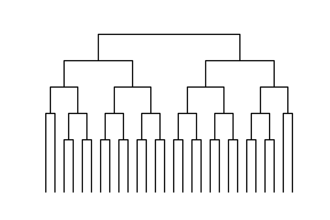
(a) Unbalanced tree

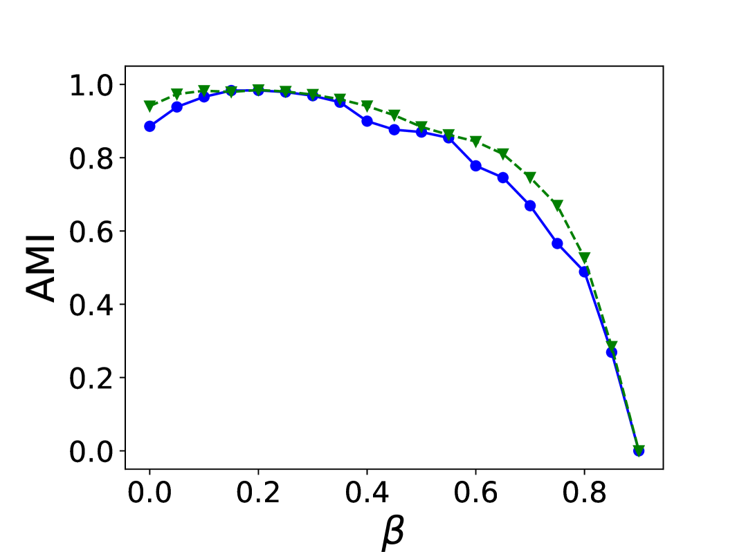
(b) AMI

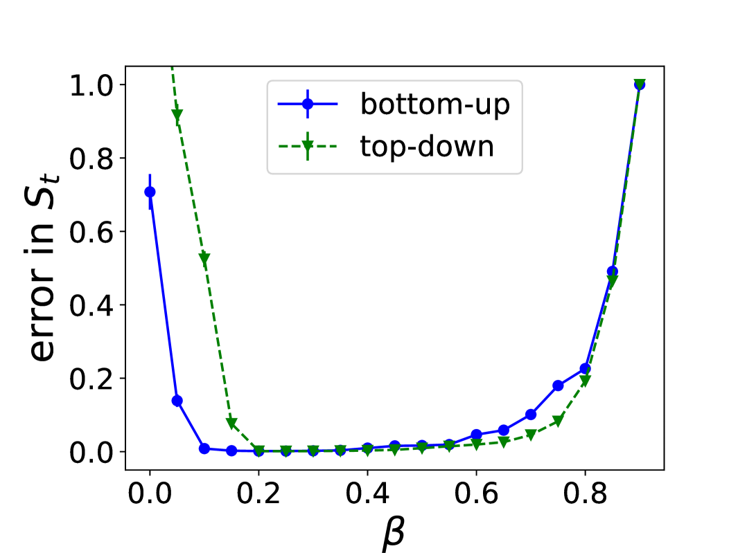
(c) Tree similarity

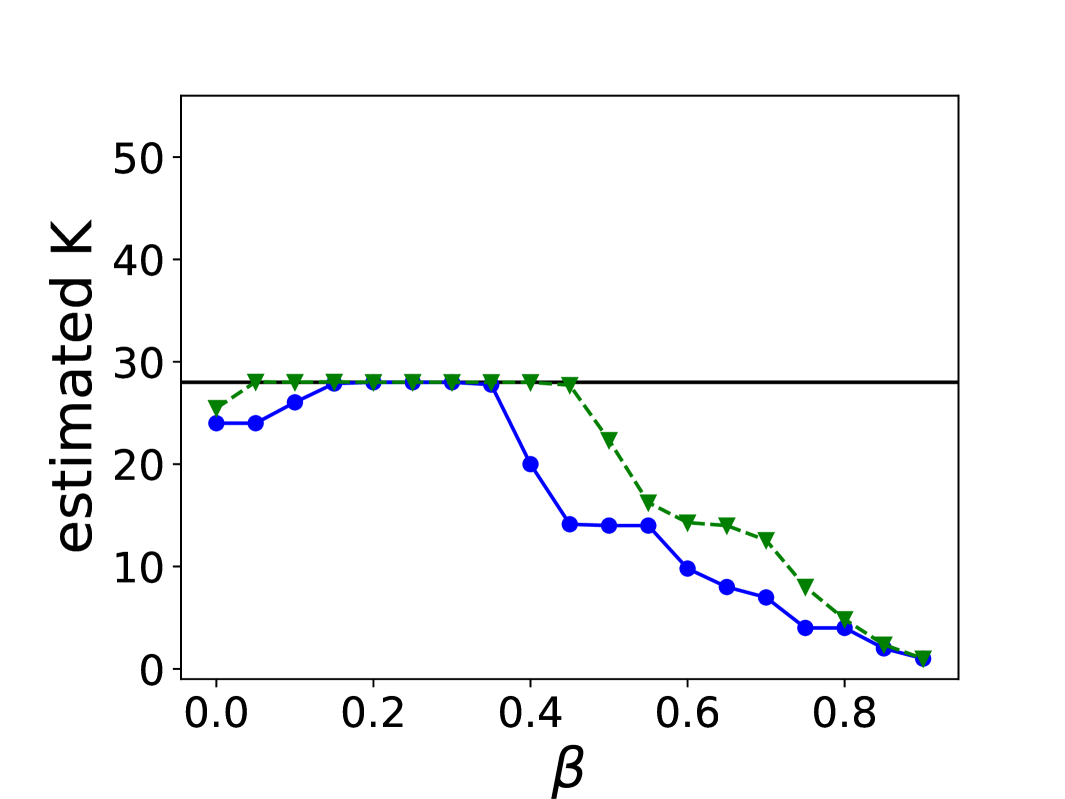
(d) Estimated $K$

Figure 9: (a) Hierarchical tree. (b)-(d) Results of the different HCD algorithms on unbalanced HSBMs whose hierarchical tree is given in Figure 9(a), and with $N=3200$ nodes and $p_{k}=64\cdot\beta^{5-k}\cdot\frac{\log{N}}{N}$. The results are averaged over 100 realizations, and error bars (vertical solid lines) show the standard error but are typically smaller than the symbols.

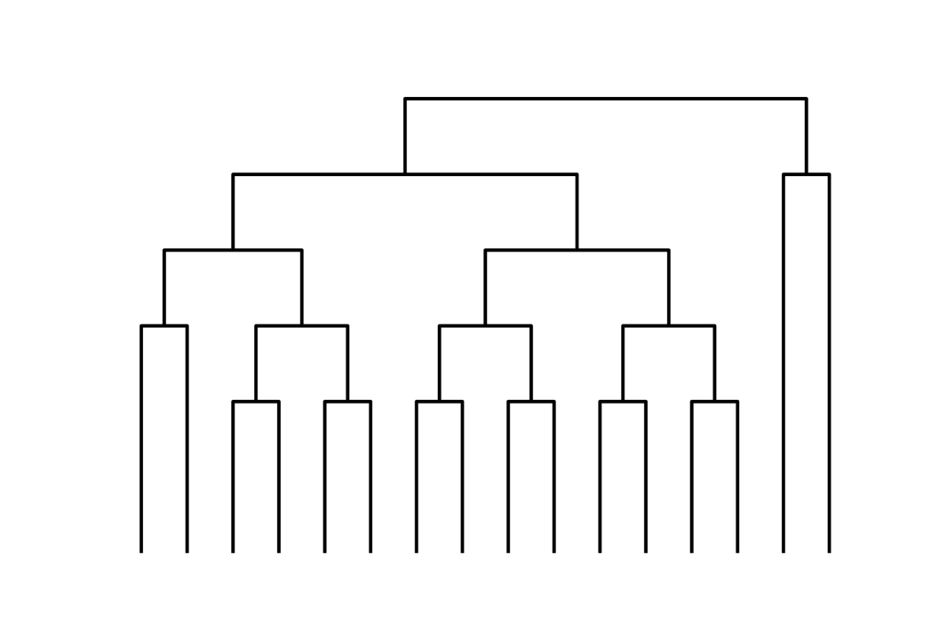
(a) Unbalanced tree

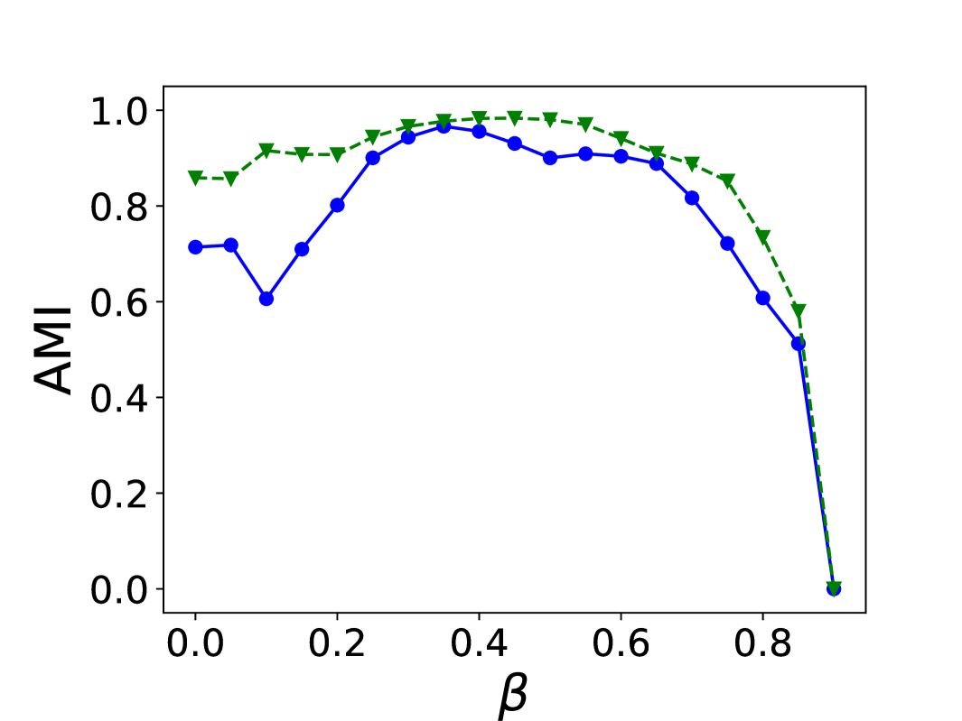
(b) AMI

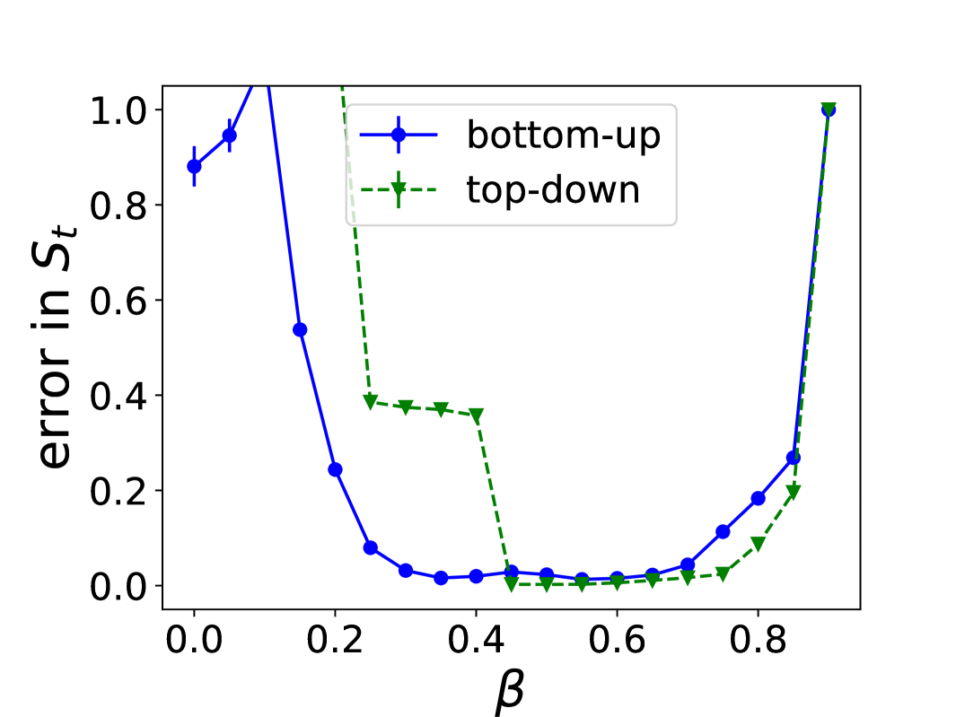
(c) Tree similarity

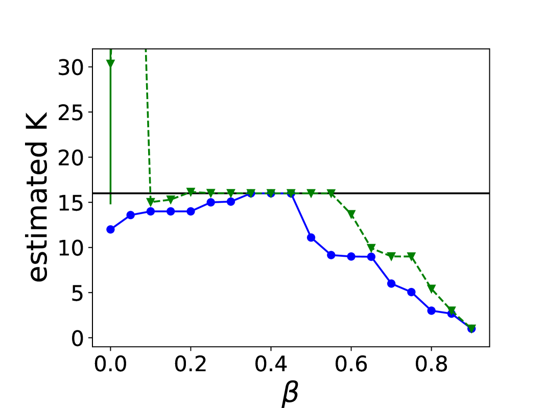
(d) Estimated $K$

Figure 10: (a) Hierarchical tree. (b)-(d) Results of the different HCD algorithms on unbalanced BTSBMs whose tree shape is given in Figure 10(a) and with $N=3200$ nodes and $p_{k}=144\cdot\beta^{5-k}\cdot\frac{\log{N}}{N}$. The results are averaged over 100 realizations, and error bars (vertical solid lines) show the standard error but are typically smaller than the symbols.

C.2 Real data sets

C.2.1 Military inter-alliance

We next consider the network of military alliances between countries. The data is provided by the Alliance Treaty Obligations and Provisions (ATOP) project [24]. We select the year 2018 (as this is the most recent year available). We define two countries as allied if they share a defensive alliance. This leads to a network of 133 countries and 1391 alliances. Some important countries such as India or Switzerland are missing as they do not share any defensive alliances with anybody. Moreover, the graph is not connected, as a small component of three countries (China, North Korea and Cuba) is disconnected from the rest of the world.

Figures 11 and 12 show the output of bottom-up and top-down algorithms. Bottom-up predicts 7 bottom communities, which represent geopolitical alliances based on political affiliation and geography (European countries, Eurasian countries, Arabic countries, Western African countries and Central/Southern African countries). The top level splits the graph’s largest connected component into 3 clusters: Western countries, Eurasian countries, and African and Middle-East countries. While some of these clusters are also recovered by top-down HCD, the separation of African countries by top-down algorithm appears worse.

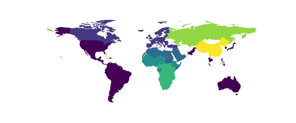
(a) Bottom level.

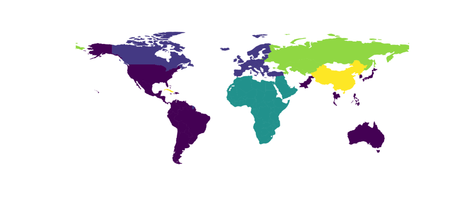
(b) Middle level (after 2 merges).

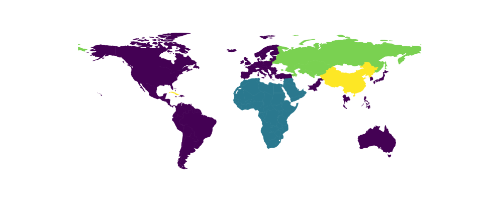
(c) Top level (after 3 merges).

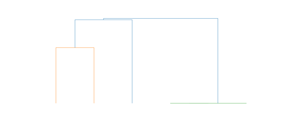
(d) Dendrogram.

Figure 11: Output of bottom-up algorithm on the military alliance network. The dendrogram does not show the disconnected component (China, Cuba, North Korea).

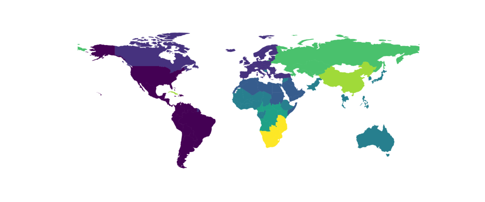
(a) Bottom level (8 clusters).

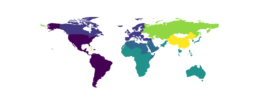
(b) Middle level (6 clusters).

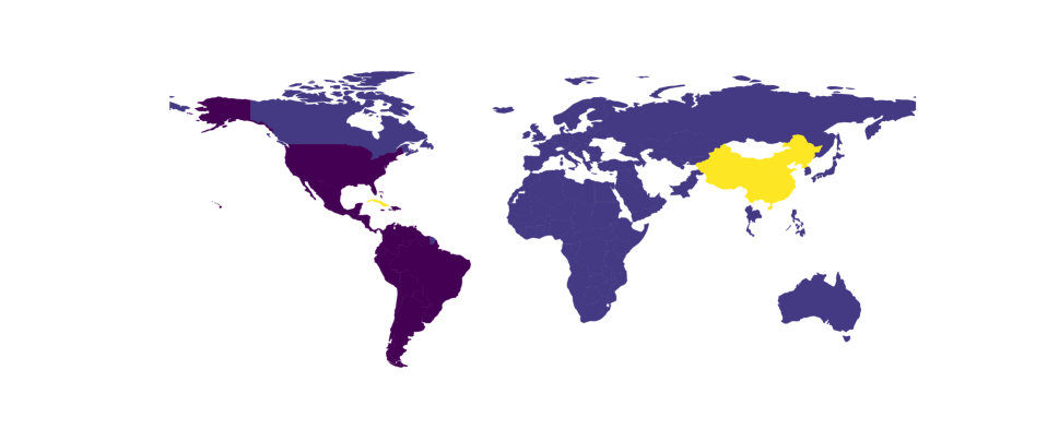
(c) Top level (3 clusters).

(d) Dendrogram.

Figure 12: Output of top-down algorithm on the military alliance network. The dendrogram does not show the disconnected component (China, Cuba, North Korea).

C.2.2 Football data set

We also test HCD algorithms on the United States college (American) football dataset [18]. This network represents the schedule of Division I games for the 2000 season. Each node in the network corresponds to a college football team, and edges represent the regular-season games between the teams. The teams are categorized into 11 conferences, in which games are more frequent between the members. Each conference has 8 to 12 teams. We exclude the ”independent” teams which do not belong to any conferences. Since the original community labels appear to be based on the 2001 season, while the edges represent the games played during the 2000 season, we proceed to the same correction as in [15].

The results obtained by the different HCD algorithms are given in Figure 13. First, we observe that all the algorithms perform well (AMI for bottom-up, top-down, Paris, and Bayesian are respectively 0.962, $0.892$, 0.965, and 0.976). However, top-down has more errors than the other algorithms. Interestingly, bottom-up, top-down, and Bayesian algorithms predict 10 clusters (more precisely, Bayesian detects 10.1 communities averaged over 100 runs), as they tend to infer Big West and Mountain West conferences as a single cluster. Finally, we can restore some geographical proximity among conferences from the hierarchy inferred by bottom-up. For example, Conference USA is composed of teams located in the Southern United States, while the Southeastern Conference’s member institutions are located primarily in the South Central and Southeastern United States. Another example is that teams belonging to Pacific Ten, Big West, and Mountain West are all located in the West, and these conferences are also close in the bottom-up dendrogram.

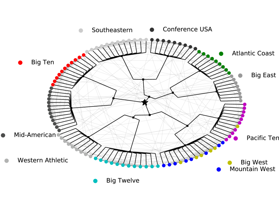
(a) bottom-up

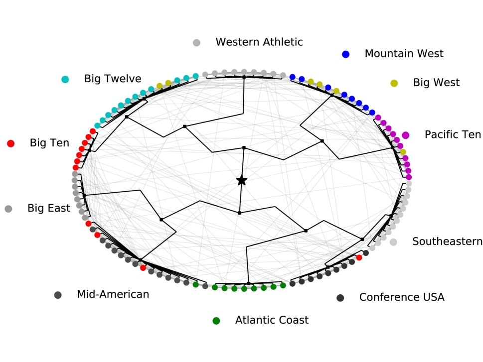
(b) top-down

Figure 13: Output of bottom-up and top-down algorithms on the football data set. The colours correspond to conferences, and grey edges indicate having regular-season games between the two teams. The hierarchical tree is drawn in black, and its root is marked by a star symbol.

References

- AD [22] Konstantin Avrachenkov and Maximilien Dreveton. Statistical Analysis of Networks. Boston-Delft: now publishers, 10 2022.
- ADL [22] Konstantin Avrachenkov, Maximilien Dreveton, and Lasse Leskelä. Community recovery in non-binary and temporal stochastic block models. arXiv e-prints, page arXiv:2008.04790, 2022.
- [3] Emmanuel Abbe and Colin Sandon. Community detection in general stochastic block models: Fundamental limits and efficient algorithms for recovery. In 2015 IEEE 56th Annual Symposium on Foundations of Computer Science, pages 670–688, Los Alamitos, CA, USA, 2015. IEEE Computer Society.
- [4] Emmanuel Abbe and Colin Sandon. Recovering communities in the general stochastic block model without knowing the parameters. Advances in neural information processing systems, 28, 2015.
- BCGH [18] Thomas Bonald, Bertrand Charpentier, Alexis Galland, and Alexandre Hollocou. Hierarchical graph clustering using node pair sampling. In MLG 2018 - 14th International Workshop on Mining and Learning with Graphs, London, 2018.
- BGLL [08] Vincent D Blondel, Jean-Loup Guillaume, Renaud Lambiotte, and Etienne Lefebvre. Fast unfolding of communities in large networks. Journal of statistical mechanics: theory and experiment, 2008(10):P10008, 2008.
- BXKS [11] Sivaraman Balakrishnan, Min Xu, Akshay Krishnamurthy, and Aarti Singh. Noise thresholds for spectral clustering. Advances in Neural Information Processing Systems, 24, 2011.
- CAKMT [17] Vincent Cohen-Addad, Varun Kanade, and Frederik Mallmann-Trenn. Hierarchical clustering beyond the worst-case. In Advances in Neural Information Processing Systems, volume 30, Red Hook, NY, USA, 2017. Curran Associates, Inc.
- CAKMTM [19] Vincent Cohen-Addad, Varun Kanade, Frederik Mallmann-Trenn, and Claire Mathieu. Hierarchical clustering: Objective functions and algorithms. Journal of the ACM (JACM), 66(4):1–42, 2019.
- CHCL [11] Cheng-Shang Chang, Chin-Yi Hsu, Jay Cheng, and Duan-Shin Lee. A general probabilistic framework for detecting community structure in networks. In 2011 Proceedings IEEE INFOCOM, pages 730–738. IEEE, 2011.
- CNM [04] Aaron Clauset, Mark EJ Newman, and Cristopher Moore. Finding community structure in very large networks. Physical review E, 70(6):066111, 2004.
- Das [16] Sanjoy Dasgupta. A cost function for similarity-based hierarchical clustering. In Proceedings of the Forty-Eighth Annual ACM Symposium on Theory of Computing, STOC ’16, page 118–127, New York, NY, USA, 2016. Association for Computing Machinery.
- DCT [21] Lorenzo Dall’Amico, Romain Couillet, and Nicolas Tremblay. A unified framework for spectral clustering in sparse graphs. J. Mach. Learn. Res., 22:217–1, 2021.
- DHKM [06] Anirban Dasgupta, John Hopcroft, Ravi Kannan, and Pradipta Mitra. Spectral clustering by recursive partitioning. In European Symposium on Algorithms, pages 256–267. Springer, 2006.
- Eva [10] Tim S Evans. Clique graphs and overlapping communities. Journal of Statistical Mechanics: Theory and Experiment, 2010(12):P12037, 2010.
- For [10] Santo Fortunato. Community detection in graphs. Physics reports, 486(3-5):75–174, 2010.
- GBW [22] Lucy L. Gao, Jacob Bien, and Daniela Witten. Selective inference for hierarchical clustering. Journal of the American Statistical Association, 0(0):1–11, 2022.
- GN [02] Michelle Girvan and Mark EJ Newman. Community structure in social and biological networks. Proceedings of the national academy of sciences, 99(12):7821–7826, 2002.
- GV [16] Olivier Guédon and Roman Vershynin. Community detection in sparse networks via grothendieck’s inequality. Probability Theory and Related Fields, 165(3-4):1025–1049, 2016.
- HSH+ [10] Jianbin Huang, Heli Sun, Jiawei Han, Hongbo Deng, Yizhou Sun, and Yaguang Liu. Shrink: a structural clustering algorithm for detecting hierarchical communities in networks. In Proceedings of the 19th ACM international conference on Information and knowledge management, pages 219–228, 2010.
- Lei [20] Lihua Lei. Unified eigenspace perturbation theory for symmetric random matrices, arXiv:1909.04798v2, 2020.
- LLB+ [22] Tianxi Li, Lihua Lei, Sharmodeep Bhattacharyya, Koen Van den Berge, Purnamrita Sarkar, Peter J Bickel, and Elizaveta Levina. Hierarchical community detection by recursive partitioning. Journal of the American Statistical Association, 117(538):951–968, 2022.
- LLL [21] Lihua Lei, Xiaodong Li, and Xingmei Lou. Consistency of spectral clustering on hierarchical stochastic block models, arXiv:2004.14531v2, 2021.
- LRML [02] Brett Leeds, Jeffrey Ritter, Sara Mitchell, and Andrew Long. Alliance treaty obligations and provisions, 1815-1944. International Interactions, 28(3):237–260, 2002.
- LTA+ [16] Vince Lyzinski, Minh Tang, Avanti Athreya, Youngser Park, and Carey E Priebe. Community detection and classification in hierarchical stochastic blockmodels. IEEE Transactions on Network Science and Engineering, 4(1):13–26, 2016.
- MC [17] Fionn Murtagh and Pedro Contreras. Algorithms for hierarchical clustering: an overview, ii. Wiley Interdisciplinary Reviews: Data Mining and Knowledge Discovery, 7(6):e1219, 2017.
- MFB [15] Rossana Mastrandrea, Julie Fournet, and Alain Barrat. Contact patterns in a high school: A comparison between data collected using wearable sensors, contact diaries and friendship surveys. PLOS ONE, 10(9):1–26, 09 2015.
- MNS [16] Elchanan Mossel, Joe Neeman, and Allan Sly. Consistency thresholds for the planted bisection model. Electronic Journal of Probability, 21(none):1 – 24, 2016.
- Moj [77] Richard Mojena. Hierarchical grouping methods and stopping rules: an evaluation. The Computer Journal, 20(4):359–363, 1977.
- New [04] Mark EJ Newman. Fast algorithm for detecting community structure in networks. Physical review E, 69(6):066133, 2004.
- New [18] Mark EJ Newman. Networks. Oxford University Press, 07 2018.
- PL [05] Pascal Pons and Matthieu Latapy. Computing communities in large networks using random walks. In International symposium on computer and information sciences, pages 284–293. Springer, 2005.
- RCC+ [04] Filippo Radicchi, Claudio Castellano, Federico Cecconi, Vittorio Loreto, and Domenico Parisi. Defining and identifying communities in networks. Proceedings of the national academy of sciences, 101(9):2658–2663, 2004.
- SDYB [12] Michael T Schaub, Jean-Charles Delvenne, Sophia N Yaliraki, and Mauricio Barahona. Markov dynamics as a zooming lens for multiscale community detection: non clique-like communities and the field-of-view limit. PloS one, 7(2):e32210, 2012.
- SKZ [14] Alaa Saade, Florent Krzakala, and Lenka Zdeborová. Spectral clustering of graphs with the bethe hessian. Advances in Neural Information Processing Systems, 27, 2014.
- VEB [09] Nguyen Xuan Vinh, Julien Epps, and James Bailey. Information theoretic measures for clusterings comparison: Is a correction for chance necessary? In Proceedings of the 26th Annual International Conference on Machine Learning, ICML ’09, page 1073–1080, New York, NY, USA, 2009. Association for Computing Machinery.
- VEH [14] Tim Van Erven and Peter Harremos. Rényi divergence and kullback-leibler divergence. IEEE Transactions on Information Theory, 60(7):3797–3820, 2014.
- YP [16] Se-Young Yun and Alexandre Proutiere. Optimal cluster recovery in the labeled stochastic block model. Advances in Neural Information Processing Systems, 29, 2016.